Surface deformations and wave generation by wind blowingover a viscous liquid

A. Paquier,1 F. Moisy,1 and M. Rabaud1

Laboratoire FAST, Univ. Paris-Sud, CNRS, Universite Paris-Saclay, F-91405, Orsay,France.

(Dated: 21 September 2015)

We investigate experimentally the early stage of the generation of waves by a tur-bulent wind at the surface of a viscous liquid. The spatio-temporal structure ofthe surface deformation is analyzed by the optical method Free Surface SyntheticSchlieren, which allows for time-resolved measurements with a micrometric accu-racy. Because of the high viscosity of the liquid, the flow induced by the turbulentwind in the liquid remains laminar, with weak surface drift velocity. Two regimesof deformation of the liquid-air interface are identified. In the first regime, at lowwind speed, the surface is dominated by rapidly propagating disorganized wrin-kles, elongated in the streamwise direction, which can be interpreted as the surfaceresponse to the pressure fluctuations advected by the turbulent airflow. The am-plitude of these deformations increases approximately linearly with wind velocityand are essentially independent of the fetch (distance along the channel). Above athreshold in wind speed, the perturbations organize themselves spatially into quasiparallel waves perpendicular to the wind direction with their amplitude increasingdownstream. In this second regime, the wave amplitude increases with wind speedbut far more quickly than in the first regime.

PACS numbers: 45.35.-i,47.54.-r

I. INTRODUCTION

Understanding the generation of surface waves under the action of wind is an old problemwhich is of primary interest for wave forecasting and to evaluate air-sea exchanges of heat,mass and momentum on Earth1,2 or on natural satellites.3,4 It is also important in engi-neering applications involving liquid and gas transport in pipes.5 Despite the considerableliterature on the subject, the physical mechanism for the onset of the first ripples at low windvelocity is still not fully understood. Russell,6 as quoted by Kelvin,7 nicely described thefirst regime where a very slight wind first destroys the perfect mirror reflection of the watersurface, followed by a second regime for slightly larger wind where waves are observed. Thefirst attempt to explain the wind-wave formation was proposed by Helmholtz and Kelvin,7,8

and the Kelvin-Helmholtz instability is now a paradigm for instabilities in fluid mechan-ics. However, Kelvin was aware of the discrepancy between the predicted critical wind of6.6 m s−1 and the commonly observed minimal wind of the order of 1 m s−1 for the firstvisible ripples on a calm sea.9 He ascribed this discrepancy to viscous effects, which werenot taken into account in the model. Since then, numerous attempts to better predict theonset of wind waves were proposed, still with limited success.

Among the large body of literature on the subject, pioneering theoretical contributions arethose of Phillips10 and Miles.11 In an enlightening paper, Phillips10 analyzed how pressurefluctuations in the turbulent air boundary layer could deform an otherwise inviscid fluidat rest. He suggested that the pressure perturbations whose size and phase velocity matchthat of the waves are selectively amplified by a resonance mechanism, and obtained a lineargrowth in time of the squared wave amplitude. The same year, Miles11 proposed anothermechanism based on the shear flow instability of the mean air velocity profile, ignoringviscosity, surface tension, drift of the liquid and turbulent fluctuations. From a temporalstability analysis, he showed that the boundary layer in the air is unstable if the curvature ofthe velocity profile is negative at the critical height at which air moves at the phase velocityof the waves, resulting in an exponential growth in time of the wave amplitude. An effortto classify the various instability mechanisms in parallel two-phase flow, including Miles’, isproposed in the review by Boomkamp and Miesen.12

Since then, many attempts have been made to test these predictions13–17 or to improvethese models,18–22 with no definitive conclusion at the moment. While several experimentswere devoted to determine the temporal growth of the wave after a rapid initiation of the

arX

iv:1

509.

0546

7v1

[ph

ysic

s.fl

u-dy

n] 1

7 Se

p 20

15

2

x

z

0

L = 1.5 m

H

dot pattern

camera

honeycomb

h

Uafan

flexiblecoupling

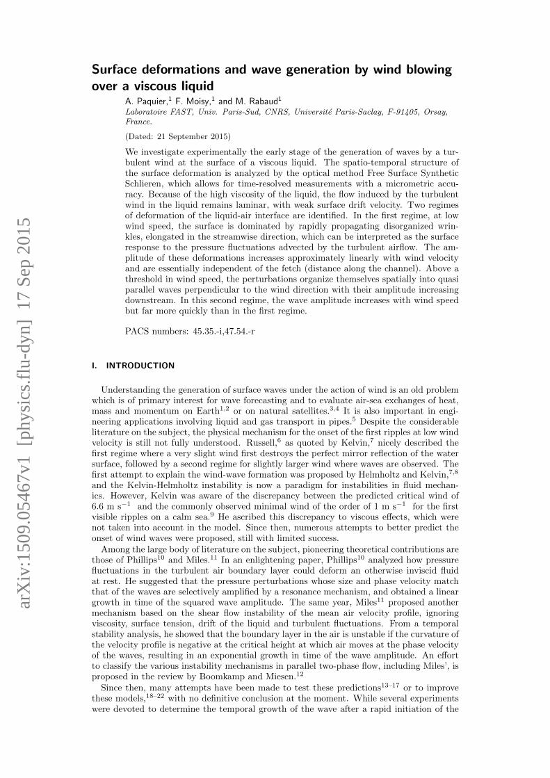
FIG. 1. Experimental setup. The wave tank and the wind tunnel are connected to the upstreamair flow via a flexible coupling to minimize transmission of vibrations induced by the centrifugalfan. The surface deformations are measured by Free-Surface Synthetic Schlieren, by imaging fromabove a pattern of random dots located below the liquid tank.

wind,23–25 other tested the amplification by wind of mechanically generated waves26–30 orthe wave formation by a laminar air flow.30–32 Since the boundary layers in both fluids aregenerally turbulent in the case of the air-water interface,33–36 some authors simplified theproblem by considering more viscous liquids.27,31,37–39 With an airflow above a liquid moreviscous than water, the wave onset is larger and, paradoxically, in better agreement withthe inviscid Kelvin-Helmholtz prediction.31,38,40

Rapid progresses in numerical simulations have made it possible now to address the cou-pled turbulent flows of air and water and their effect on the interface, and to access thepressure and stress fields hardly measurable in experiments.41 On the experimental side, re-cent improvements in optical methods have opened the possibility to access experimentallythe spatio-temporal structures of the waves with unprecedented resolution.42,43

In the present work, we take advantage of this technical improvement to analyze theearly stage of wave formation at the surface of a viscous liquid. Surface deformations aremeasured with a vertical resolution better than one micrometer using Free-surface SyntheticSchlieren,42 a time-resolved optical method based on the refraction of a pattern located belowthe fluid interface. Working with a viscous liquid has two advantages: first, the flow in theliquid remains laminar and essentially unidirectional with a limited surface drift; second,the perturbations of the interface that are not amplified by an instability mechanism arerapidly damped, so the surface deformations at low wind velocity are expected to be thelocal response in space and time to the instantaneous pressure fluctuations in the air. Ourresults clearly exhibit two wave regimes: (i) at low wind velocity, small disordered surfacedeformations that we call ”wrinkles” first appear, elongated in the streamwise direction,with amplitude growing slowly with the wind velocity but with no significant evolution withfetch (the distance upon which the air blows on the liquid); (ii) above a well defined windvelocity, a regular pattern of gravity-capillary waves appears, with crests normal to the winddirection and amplitude rapidly increasing with wind velocity and fetch.

II. EXPERIMENTAL SET-UP

A. Liquid tank and wind tunnel

The experimental set-up is sketched in Fig. 1. It is composed of a fully transparentPlexiglas rectangular tank of length L = 1.5 m, width W = 296 mm, and depth h = 35 mm,fitted to the bottom of a horizontal channel of rectangular cross-section. The channel widthis identical to that of the tank, its height is H = 105 mm, with two horizontal floors oflength 26 cm before and after the tank. The tank is filled with a water-glycerol mixture,such that the surface of the liquid precisely coincides with the bottom of the wind tunnel.

Air is injected upstream by a centrifugal fan through a honeycomb and a convergent (ratio2.4 in the vertical direction). To minimize transmission of vibrations induced by the fan, the

3

wind-tunnel is mounted on a heavy granite table and connected to the upstream channel viaa flexible coupling. Residual vibrations induce surface deformations less than 1 µm. Thewind velocity Ua, measured at the center of the outlet of the wind tunnel with a hot-wireanemometer, can be adjusted in the range 1 − 10 m s−1. We define x in the streamwisedirection (fetch), y in the spanwise direction and z in the vertical direction. The origin(0,0,0) is located at the free surface at fetch 0, at mid-distance between the lateral walls.

The tank is filled with a mixture of 80% glycerol and 20% water, of density ρ = 1.20 ×103 kg m−3 at 25oC (the room temperature being regulated to this temperature). Kinematicviscosity, measured with a low shear rheometer, is ν = η/ρ = 30 × 10−6 m2 s−1 at thistemperature. The water-glycerol mixture is extremely sensitive to surface contamination,which may induce strong surface tension gradients and alter both the mean flow in the liquidand the generation of waves.14 To overcome this problem, we let the wind blow for a fewminutes, and we remove the contaminated part of the surface liquid by collecting it at theend of the tank. The procedure is repeated frequently, and in normal operating conditionsthe surface of the liquid remains clean over most of the liquid bath, with less than 30 cmof polluted surface remaining at the end of the tank. Surface tension of the clean mixture,measured with a Wilhelmy plate tensiometer, is γ = 60 ± 5 mN m−1, and the capillarywavelength is λc = 2π

√γ/ρg ' 14.2 mm. The dispersion relation for free surface waves

propagating in an inviscid liquid at rest is

ω2 =

(gk +

γ

ρk3)

tanh(kh), (1)

where ω and k are the angular frequency and wave number. Finite depth effects can be ne-glected in the present experiment: the depth correction factor, tanh(kh), is larger than 0.98for wavelength smaller than 90 mm. In spite of the large viscosity used in our experiments,viscous correction to the inviscid dispersion relation can be also neglected here:44,45 thephase velocity matches the inviscid prediction to better than 10−3 for the waves observed atonset (λ ' 30 mm). On the other hand, this large viscosity induces a strong attenuation ofthe waves. For the wave tank geometry and the typical wavelengths considered here, frictionwith the bottom and side walls is negligible, and the attenuation length for free waves isgoverned by the dissipation in the bulk,46 Lv = cg/(2νk

2), with cg(k) the group velocity.For λ ' 30 mm the attenuation length is Lv ' 60 mm, indicating that a free disturbance atthis wavelength cannot propagate over a distance much larger than a few wavelengths. Asa consequence, although the tank is of limited size, reflections on the walls or at the end ofthe tank can be neglected in our experiment.

B. Wind profile

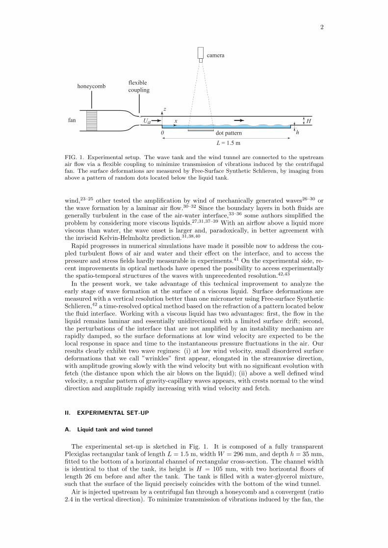
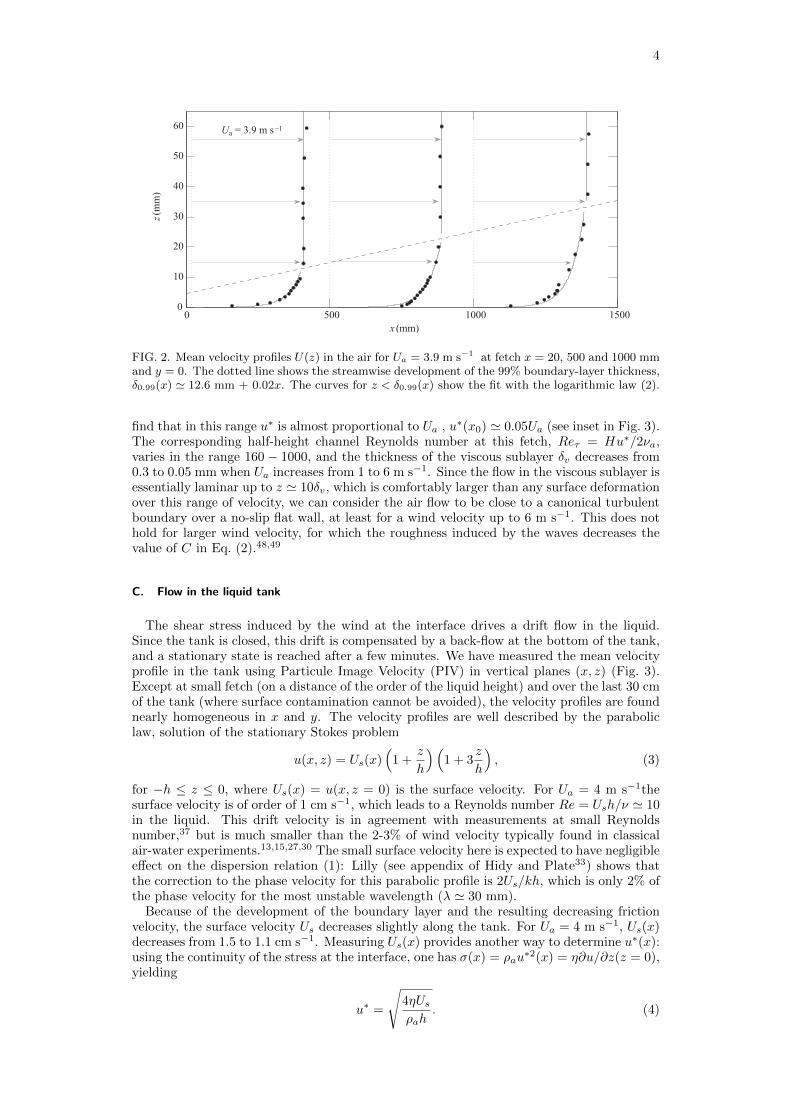
The velocity profile in the air U(z), measured using hot-wire anemometry, is shown inFig. 2 for a wind velocity Ua = 3.9 m s−1 at fetch x = 20, 500 et 1000 mm. The hot-wire(Dantec Dynamics 55P01) is 5 µm in diameter with an active length of 1.25 mm, and ismounted on a sliding arm to allow vertical motion with a 0.1 mm accuracy. The velocityprofiles show the development of the boundary layer along the channel: the thickness δ0.99,defined as the distance from the surface at which the mean velocity is 0.99Ua, increasesnearly linearly, from 12.6 mm at x = 0 to 32 mm at x = 1.0 m (slope of order of 2%).The fact that δ0.99(x) approaches the channel half-height H/2 ' 52 mm at the end of thechannel indicates that the flow becomes fully developed there.

The evolution of the friction velocity u∗(x) along the channel can be obtained by fittingthe velocity profiles for z < δ0.99(x) with the classical logarithmic law,13,47

U(x, z)

u∗(x)=

1

κln

(z

δv(x)

)+ C, (2)

with κ ' 0.4 the Karman constant, C = 5, and δv(x) = νa/u∗(x) the thickness of the viscous

sublayer. We find u∗ to slightly decrease with fetch: for Ua = 3.9 m s−1, u∗ decreases from0.22 m s−1 at x ' 0 down to 0.17 m s−1 at x = 1 m. Accordingly, δv(x) slightly increaseswith fetch, from 0.07 to 0.09 mm.

The procedure is repeated for different wind velocities at a fixed fetch, x0 = 500 mm.Measurements are restricted to Ua < 6 m s−1, when the surface deformations remain weak(less than 10 µm), because the hot-wire could not be positioned too close to the liquid. We

4

0 500 1000 15000

10

20

30

40

50

60

x (mm)

z (m

m)

Ua = 3.9 m s−1

FIG. 2. Mean velocity profiles U(z) in the air for Ua = 3.9 m s−1 at fetch x = 20, 500 and 1000 mmand y = 0. The dotted line shows the streamwise development of the 99% boundary-layer thickness,δ0.99(x) ' 12.6 mm + 0.02x. The curves for z < δ0.99(x) show the fit with the logarithmic law (2).

find that in this range u∗ is almost proportional to Ua , u∗(x0) ' 0.05Ua (see inset in Fig. 3).The corresponding half-height channel Reynolds number at this fetch, Reτ = Hu∗/2νa,varies in the range 160 − 1000, and the thickness of the viscous sublayer δv decreases from0.3 to 0.05 mm when Ua increases from 1 to 6 m s−1. Since the flow in the viscous sublayer isessentially laminar up to z ' 10δv, which is comfortably larger than any surface deformationover this range of velocity, we can consider the air flow to be close to a canonical turbulentboundary over a no-slip flat wall, at least for a wind velocity up to 6 m s−1. This does nothold for larger wind velocity, for which the roughness induced by the waves decreases thevalue of C in Eq. (2).48,49

C. Flow in the liquid tank

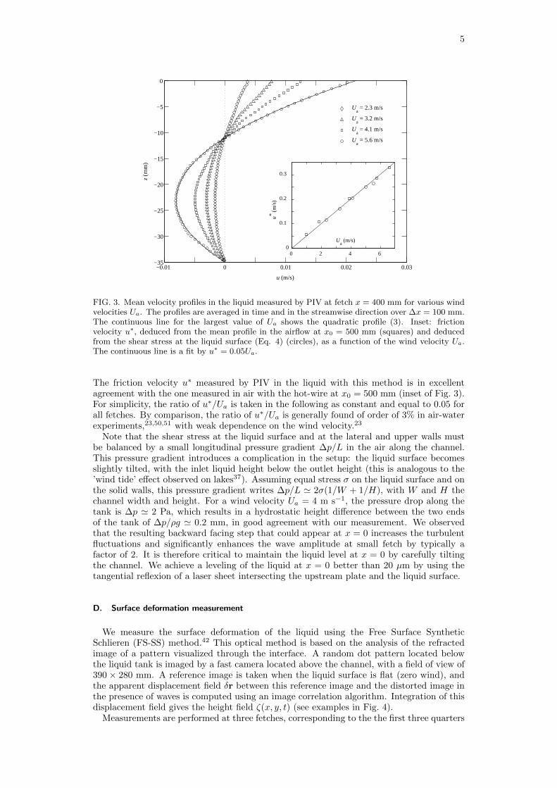
The shear stress induced by the wind at the interface drives a drift flow in the liquid.Since the tank is closed, this drift is compensated by a back-flow at the bottom of the tank,and a stationary state is reached after a few minutes. We have measured the mean velocityprofile in the tank using Particule Image Velocity (PIV) in vertical planes (x, z) (Fig. 3).Except at small fetch (on a distance of the order of the liquid height) and over the last 30 cmof the tank (where surface contamination cannot be avoided), the velocity profiles are foundnearly homogeneous in x and y. The velocity profiles are well described by the paraboliclaw, solution of the stationary Stokes problem

u(x, z) = Us(x)(

1 +z

h

)(1 + 3

z

h

), (3)

for −h ≤ z ≤ 0, where Us(x) = u(x, z = 0) is the surface velocity. For Ua = 4 m s−1thesurface velocity is of order of 1 cm s−1, which leads to a Reynolds number Re = Ush/ν ' 10in the liquid. This drift velocity is in agreement with measurements at small Reynoldsnumber,37 but is much smaller than the 2-3% of wind velocity typically found in classicalair-water experiments.13,15,27,30 The small surface velocity here is expected to have negligibleeffect on the dispersion relation (1): Lilly (see appendix of Hidy and Plate33) shows thatthe correction to the phase velocity for this parabolic profile is 2Us/kh, which is only 2% ofthe phase velocity for the most unstable wavelength (λ ' 30 mm).

Because of the development of the boundary layer and the resulting decreasing frictionvelocity, the surface velocity Us decreases slightly along the tank. For Ua = 4 m s−1, Us(x)decreases from 1.5 to 1.1 cm s−1. Measuring Us(x) provides another way to determine u∗(x):using the continuity of the stress at the interface, one has σ(x) = ρau

∗2(x) = η∂u/∂z(z = 0),yielding

u∗ =

√4ηUsρah

. (4)

5

−0.01 0 0.01 0.02 0.03

−30

−25

−20

−15

−10

−5

0

u (m/s)

z (m

m)

−35

Ua = 2.3 m/s

Ua = 3.2 m/s

Ua = 4.1 m/s

Ua = 5.6 m/s

0 2 4 60

0.1

0.2

0.3

Ua (m/s)

u* (m

/s)

FIG. 3. Mean velocity profiles in the liquid measured by PIV at fetch x = 400 mm for various windvelocities Ua. The profiles are averaged in time and in the streamwise direction over ∆x = 100 mm.The continuous line for the largest value of Ua shows the quadratic profile (3). Inset: frictionvelocity u∗, deduced from the mean profile in the airflow at x0 = 500 mm (squares) and deducedfrom the shear stress at the liquid surface (Eq. 4) (circles), as a function of the wind velocity Ua.The continuous line is a fit by u∗ = 0.05Ua.

The friction velocity u∗ measured by PIV in the liquid with this method is in excellentagreement with the one measured in air with the hot-wire at x0 = 500 mm (inset of Fig. 3).For simplicity, the ratio of u∗/Ua is taken in the following as constant and equal to 0.05 forall fetches. By comparison, the ratio of u∗/Ua is generally found of order of 3% in air-waterexperiments,23,50,51 with weak dependence on the wind velocity.23

Note that the shear stress at the liquid surface and at the lateral and upper walls mustbe balanced by a small longitudinal pressure gradient ∆p/L in the air along the channel.This pressure gradient introduces a complication in the setup: the liquid surface becomesslightly tilted, with the inlet liquid height below the outlet height (this is analogous to the’wind tide’ effect observed on lakes37). Assuming equal stress σ on the liquid surface and onthe solid walls, this pressure gradient writes ∆p/L ' 2σ(1/W + 1/H), with W and H thechannel width and height. For a wind velocity Ua = 4 m s−1, the pressure drop along thetank is ∆p ' 2 Pa, which results in a hydrostatic height difference between the two endsof the tank of ∆p/ρg ' 0.2 mm, in good agreement with our measurement. We observedthat the resulting backward facing step that could appear at x = 0 increases the turbulentfluctuations and significantly enhances the wave amplitude at small fetch by typically afactor of 2. It is therefore critical to maintain the liquid level at x = 0 by carefully tiltingthe channel. We achieve a leveling of the liquid at x = 0 better than 20 µm by using thetangential reflexion of a laser sheet intersecting the upstream plate and the liquid surface.

D. Surface deformation measurement

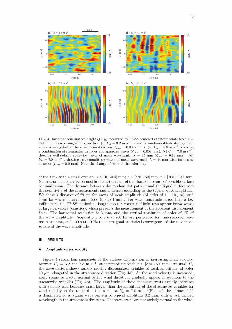
We measure the surface deformation of the liquid using the Free Surface SyntheticSchlieren (FS-SS) method.42 This optical method is based on the analysis of the refractedimage of a pattern visualized through the interface. A random dot pattern located belowthe liquid tank is imaged by a fast camera located above the channel, with a field of view of390 × 280 mm. A reference image is taken when the liquid surface is flat (zero wind), andthe apparent displacement field δr between this reference image and the distorted image inthe presence of waves is computed using an image correlation algorithm. Integration of thisdisplacement field gives the height field ζ(x, y, t) (see examples in Fig. 4).

Measurements are performed at three fetches, corresponding to the the first three quarters

6

ζ (mm

)

(a) Ua = 3.2 m s-1wind

(b) Ua = 5.9 m s-1

(c) Ua = 7.0 m s-1 (d) Ua = 7.8 m s-1

ζ (mm

)

ζ (mm

)ζ (m

m)

x (mm)400 500 600 700

y (m

m)

-100

0

100

-0.01

0

0.01

x (mm)400 500 600 700

y (m

m)

-100

0

100

-0.025

0

0.025

x (mm)400 500 600 700

y (m

m)

-100

0

100

-1.5

0

1.5

x (mm)400 500 600 700

y (m

m)

-100

0

100

-0.25

0

0.25

FIG. 4. Instantaneous surface height ζ(x, y) measured by FS-SS centered at intermediate fetch x =570 mm, at increasing wind velocities. (a) Ua = 3.2 m s−1, showing small-amplitude disorganizedwrinkles elongated in the streamwise direction (ζrms = 0.0032 mm). (b) Ua = 5.9 m s−1, showinga combination of streamwise wrinkles and spanwise waves (ζrms = 0.009 mm). (c) Ua = 7.0 m s−1,showing well-defined spanwise waves of mean wavelength λ = 35 mm (ζrms = 0.12 mm). (d)Ua = 7.8 m s−1, showing large-amplitude waves of mean wavelength λ = 44 mm with increasingdisorder (ζrms = 0.6 mm). Note the change of scale in the color map.

of the tank with a small overlap: x ∈ [10, 400] mm; x ∈ [370, 760] mm; x ∈ [700, 1090] mm.No measurements are performed in the last quarter of the channel because of possible surfacecontamination. The distance between the random dot pattern and the liquid surface setsthe sensitivity of the measurement, and is chosen according to the typical wave amplitude.We chose a distance of 29 cm for waves of weak amplitude (of order of 1 − 10 µm), and6 cm for waves of large amplitude (up to 1 mm). For wave amplitude larger than a fewmillimeters, the FF-SS method no longer applies: crossing of light rays appear below wavesof large curvature (caustics), which prevents the measurement of the apparent displacementfield. The horizontal resolution is 3 mm, and the vertical resolution of order of 1% ofthe wave amplitude. Acquisitions of 2 s at 200 Hz are performed for time-resolved wavereconstruction, and 100 s at 10 Hz to ensure good statistical convergence of the root meansquare of the wave amplitude.

III. RESULTS

A. Amplitude versus velocity

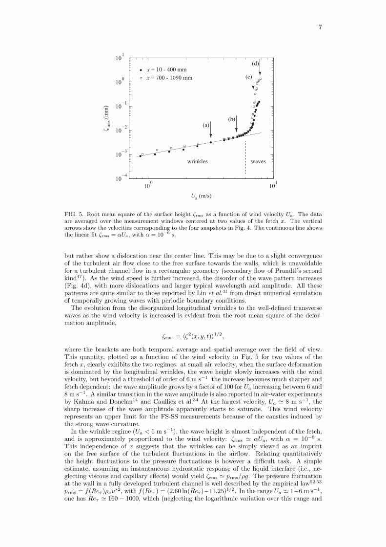
Figure 4 shows four snapshots of the surface deformation at increasing wind velocity,between Ua = 3.2 and 7.8 m s−1, at intermediate fetch x ∈ [370, 760] mm. At small Uathe wave pattern shows rapidly moving disorganized wrinkles of weak amplitude, of order10 µm, elongated in the streamwise direction (Fig. 4a). As the wind velocity is increased,noisy spanwise crests, normal to the wind direction, gradually appear in addition to thestreamwise wrinkles (Fig. 4b). The amplitude of these spanwise crests rapidly increaseswith velocity and becomes much larger than the amplitude of the streamwise wrinkles forwind velocity in the range 6 − 7 m s−1. At Ua = 7.0 m s−1(Fig. 4c) the surface fieldis dominated by a regular wave pattern of typical amplitude 0.2 mm, with a well definedwavelength in the streamwise direction. The wave crests are not strictly normal to the wind,

7

100 10110−4

10−3

10−2

10−1

100

101

Ua (m/s)

ζ rms (m

m)

(a)(b)

(c)

(d)

wrinkles waves

x = 10 - 400 mmx = 700 - 1090 mm

FIG. 5. Root mean square of the surface height ζrms as a function of wind velocity Ua. The dataare averaged over the measurement windows centered at two values of the fetch x. The verticalarrows show the velocities corresponding to the four snapshots in Fig. 4. The continuous line showsthe linear fit ζrms = αUa, with α = 10−6 s.

but rather show a dislocation near the center line. This may be due to a slight convergenceof the turbulent air flow close to the free surface towards the walls, which is unavoidablefor a turbulent channel flow in a rectangular geometry (secondary flow of Prandtl’s secondkind47). As the wind speed is further increased, the disorder of the wave pattern increases(Fig. 4d), with more dislocations and larger typical wavelength and amplitude. All thesepatterns are quite similar to those reported by Lin et al.41 from direct numerical simulationof temporally growing waves with periodic boundary conditions.

The evolution from the disorganized longitudinal wrinkles to the well-defined transversewaves as the wind velocity is increased is evident from the root mean square of the defor-mation amplitude,

ζrms = 〈ζ2(x, y, t)〉1/2,

where the brackets are both temporal average and spatial average over the field of view.This quantity, plotted as a function of the wind velocity in Fig. 5 for two values of thefetch x, clearly exhibits the two regimes: at small air velocity, when the surface deformationis dominated by the longitudinal wrinkles, the wave height slowly increases with the windvelocity, but beyond a threshold of order of 6 m s−1 the increase becomes much sharper andfetch dependent: the wave amplitude grows by a factor of 100 for Ua increasing between 6 and8 m s−1. A similar transition in the wave amplitude is also reported in air-water experimentsby Kahma and Donelan14 and Caulliez et al.34 At the largest velocity, Ua ' 8 m s−1, thesharp increase of the wave amplitude apparently starts to saturate. This wind velocityrepresents an upper limit for the FS-SS measurements because of the caustics induced bythe strong wave curvature.

In the wrinkle regime (Ua < 6 m s−1), the wave height is almost independent of the fetch,and is approximately proportional to the wind velocity: ζrms ' αUa, with α = 10−6 s.This independence of x suggests that the wrinkles can be simply viewed as an imprinton the free surface of the turbulent fluctuations in the airflow. Relating quantitativelythe height fluctuations to the pressure fluctuations is however a difficult task. A simpleestimate, assuming an instantaneous hydrostatic response of the liquid interface (i.e., ne-glecting viscous and capillary effects) would yield ζrms ' prms/ρg. The pressure fluctuationat the wall in a fully developed turbulent channel is well described by the empirical law52,53

prms = f(Reτ )ρau∗2, with f(Reτ ) = (2.60 ln(Reτ )−11.25)1/2. In the range Ua ' 1−6 m s−1,

one has Reτ ' 160− 1000, which (neglecting the logarithmic variation over this range and

8

0 200 400 600 800 1000 120010

−3

10−2

10−1

100

x (mm)

ζ rms (

mm

)

7.7 m/s

7.2 m/s7.1 m/s

6.9 m/s

6.7 m/s

6.1 m/s5.1 m/s

3.2 m/s

FIG. 6. Wave amplitude ζrms (averaged over the spanwise coordinate y and time) as a function ofthe fetch x for various wind speeds Ua. In the wrinkle regime (Ua < 6.3 m s−1) ζrms(x) is almostconstant, whereas it increases with fetch in the wave regime.

taking u∗ ' 0.05Ua) yields prms ' 0.006ρaU2a , and hence ζrms ' 0.3 − 20 µm. Although

the order of magnitude is consistent with Fig. 5, the predicted scaling (ζrms ∝ U2a ) is not

compatible with the data, suggesting that the viscous time response of the liquid must beaccounted for to describe the observed trend ζrms ∝ Ua.

B. Spatial growth rate

Contrarily to the wrinkles, which are almost independent of the fetch x, the amplitude ofthe transverse waves strongly increases with x, as shown in Fig. 6. The rms amplitude ζrms(x)is computed here using an average over y and time only. The spatial growth is approximatelyexponential at small fetch (x < 400 mm), as expected for a convective supercritical instabilityin an open flow.54 At larger fetch nonlinear effects come into play, resulting in a weakergrowth of the wave amplitude.

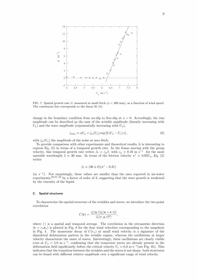
The spatial growth rate β can be estimated in the initial exponential growth regime(x < 400 mm) by fitting the squared amplitude as ζ2rms(x) ∝ exp(βx). The growth rate β,plotted in Fig. 7 as a function of the wind velocity, allows to accurately define the onset ofthe wave growth: one has β ' 0 for Ua < 6.3 m s−1, and a linear increase at larger Ua,which can be fitted by

β ' b(Ua − Uc) (5)

with Uc ' 6.3±0.1 m s−1 and b ' 11.6±0.8 s m−2. Interestingly, in the small range of fetchwhere β is computed, the waves are nearly monochromatic, with λ ' 30 mm (see Sec. III C).This indicates that the growth rate measured here, although computed from the total waveamplitude, corresponds essentially to the growth rate of the most unstable wavelength.

We note that the velocity threshold Uc ' 6.3 m s−1 turns out to be close to the (inviscid)Kelvin-Helmholtz prediction. This agreement, first noted by Francis38 for a viscous fluid, ishowever coincidental since the threshold depends on viscosity.37

An interesting question is whether the wrinkles at low wind velocity can be considered asthe seed noise for the exponential growth of the waves at larger velocity. Figure 6 indicatesthat this is apparently not the case: for Ua > 6.3 m s−1, the initial wave amplitude ζrms

extrapolated at x = 0 increases with Ua much more rapidly than the amplitude of thewrinkles; ζrms(x = 0) grows from 8 to 30µm for Ua increasing from 6.3 to 7.7 m s−1 only.This suggests that the wrinkles are not necessary for the growth of the waves. Instead, theseed noise for the waves probably results from the surface disturbance induced by the sudden

9

Ua (m s-1)

4 4.5 5 5.5 6 6.5 7 7.5 8

β (

m-1

)

-2

0

2

4

6

8

10

12

14

FIG. 7. Spatial growth rate β, measured at small fetch (x < 400 mm), as a function of wind speed.The continuous line corresponds to the linear fit (5).

change in the boundary condition from no-slip to free-slip at x = 0. Accordingly, the rmsamplitude can be described as the sum of the wrinkle amplitude (linearly increasing withUa) and the wave amplitude (exponentially increasing with Ua),

ζrms ' αUa + ζn(Ua) exp [b (Ua − Uc)x] , (6)

with ζn(Ua) the amplitude of the noise at zero fetch.To provide comparison with other experiments and theoretical results, it is interesting to

express Eq. (5) in terms of a temporal growth rate. In the frame moving with the groupvelocity, this temporal growth rate writes βt = cgβ, with cg ' 0.16 m s−1 for the mostunstable wavelength λ ' 30 mm. In terms of the friction velocity u∗ ' 0.05Ua, Eq. (5)writes

βt ' (36± 8)(u∗ − 0.31)

(in s−1). Not surprisingly, these values are smaller than the ones reported in air-waterexperiments,29,55–58 by a factor of order of 3, suggesting that the wave growth is weakenedby the viscosity of the liquid.

C. Spatial structures

To characterize the spatial structure of the wrinkles and waves, we introduce the two-pointcorrelation

C(r) =〈ζ(x, t)ζ(x + r, t)〉〈ζ(x, y, t)2〉

,

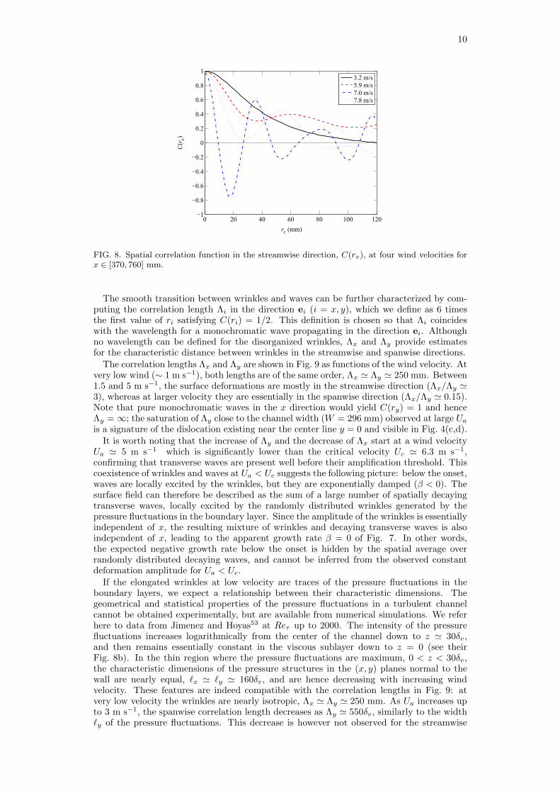
where 〈·〉 is a spatial and temporal average. The correlation in the streamwise direction(r = rxex) is plotted in Fig. 8 for the four wind velocities corresponding to the snapshotsin Fig. 4. The monotonic decay of C(rx) at small wind velocity is a signature of thedisordered deformation pattern in the wrinkle regime, whereas the oscillations at largervelocity characterize the onset of waves. Interestingly, these oscillations are clearly visibleeven at Ua = 5.9 m s−1, confirming that the transverse waves are already present in thedeformation field significantly before the critical velocity Uc ' 6.3 m s−1(see Fig. 4b). Thisindicates that the transition between the wrinkles and the waves is not sharp: both structurescan be found with different relative amplitude over a significant range of wind velocity.

10

0 20 40 60 80 100 120−1

−0.8

−0.6

−0.4

−0.2

0

0.2

0.4

0.6

0.8

1

rx (mm)

C(r x)

3.2 m/s5.9 m/s7.0 m/s7.8 m/s

FIG. 8. Spatial correlation function in the streamwise direction, C(rx), at four wind velocities forx ∈ [370, 760] mm.

The smooth transition between wrinkles and waves can be further characterized by com-puting the correlation length Λi in the direction ei (i = x, y), which we define as 6 timesthe first value of ri satisfying C(ri) = 1/2. This definition is chosen so that Λi coincideswith the wavelength for a monochromatic wave propagating in the direction ei. Althoughno wavelength can be defined for the disorganized wrinkles, Λx and Λy provide estimatesfor the characteristic distance between wrinkles in the streamwise and spanwise directions.

The correlation lengths Λx and Λy are shown in Fig. 9 as functions of the wind velocity. Atvery low wind (∼ 1 m s−1), both lengths are of the same order, Λx ' Λy ' 250 mm. Between1.5 and 5 m s−1, the surface deformations are mostly in the streamwise direction (Λx/Λy '3), whereas at larger velocity they are essentially in the spanwise direction (Λx/Λy ' 0.15).Note that pure monochromatic waves in the x direction would yield C(ry) = 1 and henceΛy =∞; the saturation of Λy close to the channel width (W = 296 mm) observed at large Uais a signature of the dislocation existing near the center line y = 0 and visible in Fig. 4(c,d).

It is worth noting that the increase of Λy and the decrease of Λx start at a wind velocityUa ' 5 m s−1 which is significantly lower than the critical velocity Uc ' 6.3 m s−1,confirming that transverse waves are present well before their amplification threshold. Thiscoexistence of wrinkles and waves at Ua < Uc suggests the following picture: below the onset,waves are locally excited by the wrinkles, but they are exponentially damped (β < 0). Thesurface field can therefore be described as the sum of a large number of spatially decayingtransverse waves, locally excited by the randomly distributed wrinkles generated by thepressure fluctuations in the boundary layer. Since the amplitude of the wrinkles is essentiallyindependent of x, the resulting mixture of wrinkles and decaying transverse waves is alsoindependent of x, leading to the apparent growth rate β = 0 of Fig. 7. In other words,the expected negative growth rate below the onset is hidden by the spatial average overrandomly distributed decaying waves, and cannot be inferred from the observed constantdeformation amplitude for Ua < Uc.

If the elongated wrinkles at low velocity are traces of the pressure fluctuations in theboundary layers, we expect a relationship between their characteristic dimensions. Thegeometrical and statistical properties of the pressure fluctuations in a turbulent channelcannot be obtained experimentally, but are available from numerical simulations. We referhere to data from Jimenez and Hoyas53 at Reτ up to 2000. The intensity of the pressurefluctuations increases logarithmically from the center of the channel down to z ' 30δv,and then remains essentially constant in the viscous sublayer down to z = 0 (see theirFig. 8b). In the thin region where the pressure fluctuations are maximum, 0 < z < 30δv,the characteristic dimensions of the pressure structures in the (x, y) planes normal to thewall are nearly equal, `x ' `y ' 160δv, and are hence decreasing with increasing windvelocity. These features are indeed compatible with the correlation lengths in Fig. 9: atvery low velocity the wrinkles are nearly isotropic, Λx ' Λy ' 250 mm. As Ua increases upto 3 m s−1, the spanwise correlation length decreases as Λy ' 550δv, similarly to the width`y of the pressure fluctuations. This decrease is however not observed for the streamwise

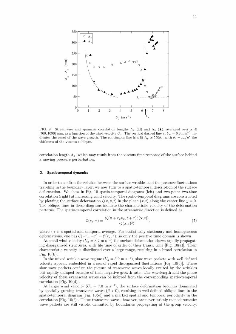
11

Ua (m s-1)

0 1 2 3 4 5 6 7 8

Λx ,

Λy

(mm

)

0

50

100

150

200

250

300

350Λ x

Λ y

λ

Uc

FIG. 9. Streamwise and spanwise correlation lengths Λx (�) and Λy (N), averaged over x ∈[700, 1090] mm, as a function of the wind velocity Ua. The vertical dashed line at Ua = 6.3 m s−1 in-dicates the onset of the wave growth. The continuous line is a fit Λy ' 550δv, with δv = νa/u

∗ thethickness of the viscous sublayer.

correlation length Λx, which may result from the viscous time response of the surface behinda moving pressure perturbation.

D. Spatiotemporal dynamics

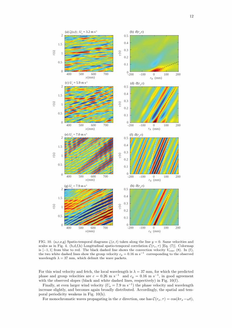
In order to confirm the relation between the surface wrinkles and the pressure fluctuationstraveling in the boundary layer, we now turn to a spatio-temporal description of the surfacedeformation. We show in Fig. 10 spatio-temporal diagrams (left) and two-point two-timecorrelation (right) at increasing wind velocity. The spatio-temporal diagrams are constructedby plotting the surface deformation ζ(x, y, t) in the plane (x, t) along the center line y = 0.The oblique lines in these diagrams indicate the characteristic velocity of the deformationpatterns. The spatio-temporal correlation in the streamwise direction is defined as

C(rx, τ) =〈ζ(x + rxex, t+ τ)ζ(x, t)〉

〈ζ(x, t)2〉, (7)

where 〈·〉 is a spatial and temporal average. For statistically stationary and homogeneousdeformations, one has C(−rx,−τ) = C(rx, τ), so only the positive time domain is shown.

At small wind velocity (Ua = 3.2 m s−1) the surface deformation shows rapidly propagat-ing disorganized structures, with life time of order of their transit time [Fig. 10(a)]. Theircharacteristic velocity is distributed over a large range, resulting in a broad correlation inFig. 10(b).

In the mixed wrinkle-wave regime (Ua = 5.9 m s−1), slow wave packets with well definedvelocity appear, embedded in a sea of rapid disorganized fluctuations [Fig. 10(c)]. Theseslow wave packets confirm the picture of transverse waves locally excited by the wrinklesbut rapidly damped because of their negative growth rate. The wavelength and the phasevelocity of these evanescent waves can be inferred from the corresponding spatio-temporalcorrelation [Fig. 10(d)].

At larger wind velocity (Ua = 7.0 m s−1), the surface deformation becomes dominatedby spatially growing transverse waves (β > 0), resulting in well defined oblique lines in thespatio-temporal diagram [Fig. 10(e)] and a marked spatial and temporal periodicity in thecorrelation [Fig. 10(f)]. These transverse waves, however, are never strictly monochromatic:wave packets are still visible, delimited by boundaries propagating at the group velocity.

12

x (mm)400 500 600 700

t (s)

0

0.5

1

1.5

2

rx (mm)-200 -100 0 100 200

τ (s)

0

0.1

0.2

0.3

0.4

0.5

x (mm)400 500 600 700

t (s)

0

0.5

1

1.5

2

-200 -100 0 100 200

τ (s)

0

0.1

0.2

0.3

0.4

0.5

x (mm)400 500 600 700

t (s)

0

0.5

1

1.5

2

-200 -100 0 100 200

τ (s)

0

0.1

0.2

0.3

0.4

0.5

x (mm)400 500 600 700

t (s)

0

0.5

1

1.5

2

-200 -100 0 100 200

τ (s)

0

0.1

0.2

0.3

0.4

0.5

(a) ζ(x,t) ; Ua = 3.2 m s-1

(c) Ua = 5.9 m s-1

(e) Ua = 7.0 m s-1

(g) Ua = 7.9 m s-1

rx (mm)

rx (mm)

rx (mm)

(b) C(rx,τ)

(d) C(rx,τ)

(f) C(rx,τ)

(h) C(rx,τ)

FIG. 10. (a,c,e,g) Spatio-temporal diagrams ζ(x, t) taken along the line y = 0. Same velocities andscales as in Fig. 4. (b,d,f,h) Longitudinal spatio-temporal correlation C(rx, τ) [Eq. (7)]. Colormapis [−1, 1] from blue to red. The black dashed line shows the convection velocity Vconv (8). In (f),the two white dashed lines show the group velocity cg = 0.16 m s−1 corresponding to the observedwavelength λ = 37 mm, which delimit the wave packets.

For this wind velocity and fetch, the local wavelength is λ = 37 mm, for which the predictedphase and group velocities are c = 0.26 m s−1 and cg = 0.16 m s−1, in good agreementwith the observed slopes (black and white dashed lines, respectively) in Fig. 10(f).

Finally, at even larger wind velocity (Ua = 7.9 m s−1) the phase velocity and wavelengthincrease slightly, and becomes again broadly distributed. Accordingly, the spatial and tem-poral periodicity weakens in Fig. 10(h).

For monochromatic waves propagating in the x direction, one has C(rx, τ) = cos(krx−ωt),

13

Ua (m s-1)

0 1 2 3 4 5 6 7 8

V conv

(m s-1

)

0

0.2

0.4

0.6

0.8

1

1.2

1.4

c

Uc

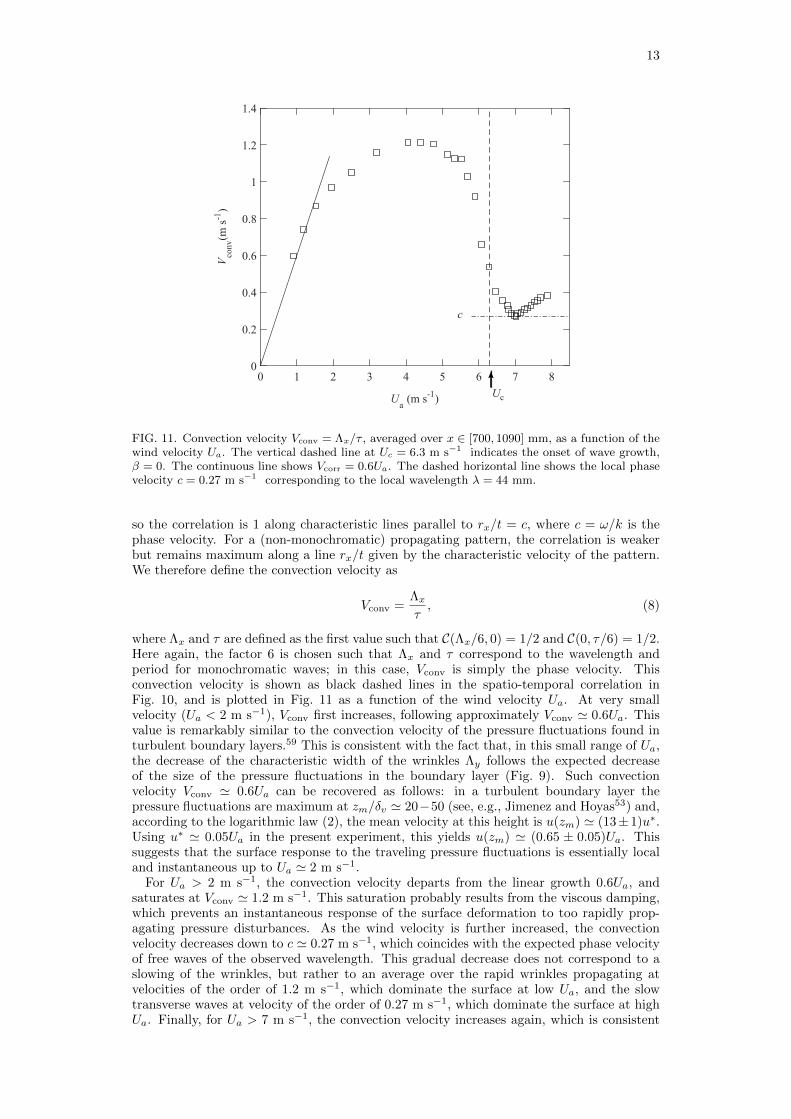
FIG. 11. Convection velocity Vconv = Λx/τ , averaged over x ∈ [700, 1090] mm, as a function of thewind velocity Ua. The vertical dashed line at Uc = 6.3 m s−1 indicates the onset of wave growth,β = 0. The continuous line shows Vcorr = 0.6Ua. The dashed horizontal line shows the local phasevelocity c = 0.27 m s−1 corresponding to the local wavelength λ = 44 mm.

so the correlation is 1 along characteristic lines parallel to rx/t = c, where c = ω/k is thephase velocity. For a (non-monochromatic) propagating pattern, the correlation is weakerbut remains maximum along a line rx/t given by the characteristic velocity of the pattern.We therefore define the convection velocity as

Vconv =Λxτ, (8)

where Λx and τ are defined as the first value such that C(Λx/6, 0) = 1/2 and C(0, τ/6) = 1/2.Here again, the factor 6 is chosen such that Λx and τ correspond to the wavelength andperiod for monochromatic waves; in this case, Vconv is simply the phase velocity. Thisconvection velocity is shown as black dashed lines in the spatio-temporal correlation inFig. 10, and is plotted in Fig. 11 as a function of the wind velocity Ua. At very smallvelocity (Ua < 2 m s−1), Vconv first increases, following approximately Vconv ' 0.6Ua. Thisvalue is remarkably similar to the convection velocity of the pressure fluctuations found inturbulent boundary layers.59 This is consistent with the fact that, in this small range of Ua,the decrease of the characteristic width of the wrinkles Λy follows the expected decreaseof the size of the pressure fluctuations in the boundary layer (Fig. 9). Such convectionvelocity Vconv ' 0.6Ua can be recovered as follows: in a turbulent boundary layer thepressure fluctuations are maximum at zm/δv ' 20−50 (see, e.g., Jimenez and Hoyas53) and,according to the logarithmic law (2), the mean velocity at this height is u(zm) ' (13± 1)u∗.Using u∗ ' 0.05Ua in the present experiment, this yields u(zm) ' (0.65 ± 0.05)Ua. Thissuggests that the surface response to the traveling pressure fluctuations is essentially localand instantaneous up to Ua ' 2 m s−1.

For Ua > 2 m s−1, the convection velocity departs from the linear growth 0.6Ua, andsaturates at Vconv ' 1.2 m s−1. This saturation probably results from the viscous damping,which prevents an instantaneous response of the surface deformation to too rapidly prop-agating pressure disturbances. As the wind velocity is further increased, the convectionvelocity decreases down to c ' 0.27 m s−1, which coincides with the expected phase velocityof free waves of the observed wavelength. This gradual decrease does not correspond to aslowing of the wrinkles, but rather to an average over the rapid wrinkles propagating atvelocities of the order of 1.2 m s−1, which dominate the surface at low Ua, and the slowtransverse waves at velocity of the order of 0.27 m s−1, which dominate the surface at highUa. Finally, for Ua > 7 m s−1, the convection velocity increases again, which is consistent

14

with the increase of the wavelength in Fig. 9. These increases do not necessarily occur forshorter fetches, implying that the wave properties change with fetch at high wind veloc-ity. Such non linear effect presents strong similarities with the wavenumber and frequencydownshift observed for wind-waves on sea, and will be investigated in future work.”

IV. CONCLUSION

In this paper, we explored the spatio-temporal properties of the first surface deforma-tions induced by a turbulent wind on a viscous fluid. New insight into the wave genera-tion mechanism is gained from spatio-temporal correlations computed from high resolutiontime-resolved measurements of the surface deformation field. At low wind velocity, rapidlypropagating disordered wrinkles of very small amplitude are observed, resulting from theresponse of the surface to the traveling pressure fluctuations in the turbulent boundary layer.Above a critical wind velocity Uc, we observe the growth of well defined propagating waves,with growth rates compatible with a convective supercritical instability. Interestingly, anintermediate regime with spatially damped waves locally excited by the wrinkles is observedbelow Uc, resulting in a smooth evolution of the characteristic lengths and velocity as thewind speed is increased. Above the onset Uc, the seed noise for the growth of the wavesis apparently not governed by the wrinkles, but rather by the perturbations at the inletboundary condition at zero fetch.

Using a liquid of large viscosity yields considerable simplification of the general problemof wave generation by wind. Although some of the present results may be relevant to themore complex air-water configuration, other are certainly specific to the large viscosity ofthe liquid. In particular, the wrinkles observed at very low wind velocity (Ua < 2 m s−1) arecompatible with a local and instantaneous response of the surface to the pressure fluctuationstraveling in the boundary layer. This simple property is not expected to hold for liquidsof lower viscosity such as water, for which the surface deformation at a given point resultsfrom the superposition of the disturbances emitted previously from all the surface. Newexperiments with varying viscosity are necessary to gain better insight into the intricaterelation between the turbulent pressure field and the surface response below the onset of thewave growth, and to characterize the spatial evolution of the waves above onset.

ACKNOWLEDGMENTS

We are grateful to H. Branger, C. Clanet, P. Clark di Leoni, B. Gallet, J. Jimenez,O Naraigh, and P. Spelt for fruitful discussions. We acknowledge A. Aubertin, L. Auffray,C. Borget, and R. Pidoux for the design and set-up of the experiment. This work is supportedby RTRA ”Triangle de la Physique”. F.M. thanks the Institut Universitaire de France.

1P. H. LeBlond and L. A. Mysak. Waves in the Ocean. Elsevier, 1981.2P. Janssen. The interaction of ocean waves and wind. Cambridge University Press, 2004.3AG Hayes, RD Lorenz, MA Donelan, M Manga, JI Lunine, T Schneider, MP Lamb, JM Mitchell, WW Fis-cher, SD Graves, et al. Wind driven capillary-gravity waves on Titan’s lakes: Hard to detect or non-existent? Icarus, 225:403–412, 2013.

4J. W. Barnes, C. Sotin, J. M. Soderblom, R. H. Brown, A. G. Hayes, M. Donelan, S. Rodriguez,S. Le Mouelic, K. H. Baines, and T. B. McCord. Cassini/vims observes rough surfaces on titan’s pungamare in specular reflection. Planetary Science, 3(1):1–17, 2014.

5G. Hewitt. Annular two-phase flow. Elsevier, 2013.6J Scott Russell. On waves. In Report of fourteenth meeting of the British Association for the Advancementof Science, York, pages 311–390, 1844.

7W. Thomson. On the waves produced by a single impulse in water of any depth, or in a dispersive medium.Proceedings of the Royal Society of London, 42:80–83, 1887.

8H. L. von Helmholtz. On discontinuous movements of fluids. Philos. Mag., 36:337, 1868.9O. Darrigol. Worlds of Flow: A History of Hydrodynamics from the Bernoullis to Prandtl. OxfordUniversity, 2005.

10O. M. Phillips. On the generation of waves by turbulent wind. J. Fluid Mech., 2(05):417–445, 1957.11J. W. Miles. On the generation of surface waves by shear flows. J. Fluid Mech., 3:185–204, 1957.12P. Boomkamp and R. Miesen. Classification of instabilities in parallel two-phase flow. International

Journal of Multiphase Flow, 22:67–88, 1996.13E. J. Plate, P. C. Chang, and G. M. Hidy. Experiments on the generation of small water waves by wind.

J. Fluid Mech., 35(4):625–656, 1969.14K. Kahma and M. A. Donelan. A laboratory study of the minimum wind speed for wind wave generation.

J. Fluid Mech., 192:339–364, 1988.

15

15D. Liberzon and L. Shemer. Experimental study of the initial stages of wind waves’ spatial evolution. J.Fluid Mech., 681:462–498, 2011.

16L. Grare, W. Peirson, H. Branger, J. Walker, J-P. Giovanangeli, and V. Makin. Growth and dissipationof wind-forced, deep-water waves. J. Fluid Mech., 722:5–50, 2013.

17T. S. Hristov, S. D. Miller, and C. A. Friehe. Dynamical coupling of wind and ocean waves throughwave-induced air flow. Nature, 422(6927):55–58, 2003.

18C. Katsis and T. R. Akylas. Wind-generated surface waves on a viscous fluid. Journal of applied mechanics,52(1):208–212, 1985.

19M. Teixeira and S.E. Belcher. On the initiation of surface waves by turbulent shear flow. Dynamics ofatmospheres and oceans, 41(1):1–27, 2006.

20G. R. Valenzuela. The growth of gravity-capillary waves in a coupled shear flow. J. Fluid Mech.,76(02):229–250, 1976.

21K. van Gastel, P. Janssen, and G. J. Komen. On phase velocity and growth rate of wind-induced gravity-capillary waves. J. Fluid Mech., 161:199–216, 1985.

22W. R. Young and C. L. Wolfe. Generation of surface waves by shear-flow instability. J. Fluid Mech.,739:276–307, 2014.

23H. Mitsuyasu and K. Rikiishi. The growth of duration-limited wind waves. J. Fluid Mech., 85(04):705–730,1978.

24S. Kawai. Generation of initial wavelets by instability of a coupled shear flow and their evolution to windwaves. J. Fluid Mech., 93(4):661–703, 1979.

25F. Veron and W. K. Melville. Experiments on the stability and transition of wind-driven water surfaces.J. Fluid Mech., 446(10):25–65, 2001.

26J. B. Bole and E. Y. Hsu. Response of gravity water waves to wind excitation. J. Fluid Mech., 35(04):657–675, 1969.

27J. Gottifredi and G. Jameson. The growth of short waves on liquid surfaces under the action of a wind.Proceedings of the Royal Society of London. A. Mathematical and Physical Sciences, 319(1538):373–397,1970.

28W. S. Wilson, M. L. Banner, R. J. Flower, J. A. Michael, and D. G. Wilson. Wind-induced growth ofmechanically generated water waves. J. Fluid Mech., 58(3):435–460, 1973.

29H. Mitsuyasu and T. Honda. Wind-induced growth of water waves. J. Fluid Mech., 123:425–442, 1982.30Y.S. Tsai, A.J. Grass, and R.R. Simons. On the spatial linear growth of gravity-capillary water waves

sheared by a laminar air flow. Physics of Fluids, 17:095101, 2005.31P. Gondret and M. Rabaud. Shear instability of two-fluid parallel flow in a Hele-Shaw cell. Phys. Fluids,

9:3267–3274, 1997.32P. Gondret, P. Ern, L. Meignin, and M. Rabaud. Experimental evidence of a nonlinear transition from

convective to absolute instability. Phys. Rev. Lett., 82:1442–1445, 1999.33G. M. Hidy and E. J. Plate. Wind action on water standing in a laboratory channel. J. Fluid Mech.,

26(04):651–687, 1966.34G. Caulliez, N. Ricci, and R. Dupont. The generation of the first visible wind waves. Physics of Fluids,

10(4):757–759, 1998.35G. Caulliez, R. Dupont, and V. Shrira. Turbulence generation in the wind-driven subsurface water flow.

In Transport at the Air-Sea Interface, pages 103–117. Springer, 2007.36S. Longo, D. Liang, L. Chiapponi, and L. Aguilera Jimenez. Turbulent flow structure in experimental

laboratory wind-generated gravity waves. Coastal Engineering, 64:1–15, 2012.37G. H. Keulegan. Wind tides in small closed channels. Journal of Research of the National Bureau of

Standards, 46:358–381, 1951.38J. Francis. Wave motions and the aerodynamic drag on a free oil surface. Phil. Mag., 45:695–702, 1954.39L. O Naraigh, P. Spelt, O.K. Matar, and T.A. Zaki. Interfacial instability in turbulent flow over a liquid

film in a channel. International Journal of Multiphase Flow, 37(7):812–830, 2011.40J. W. Miles. On the generation of surface waves by shear flows. Part 3. Kelvin-Helmholtz instability. J.

Fluid Mech., 6(04):583–598, 1959.41M.-Y. Lin, C.-H. Moeng, W.-T. Tsai, P. P. Sullivan, and S. E. Belcher. Direct numerical simulation of

wind-wave generation processes. J. Fluid Mech., 616:1–30, 2008.42F. Moisy, M. Rabaud, and K. Salsac. A synthetic schlieren method for the measurement of the topography

of a liquid interface. Exp. Fluids, 46:1021–1036, 2009.43D. Kiefhaber, S. Reith, R. Rocholz, and B. Jahne. High-speed imaging of short wind waves by shape from

refraction. Journal of the European Optical Society-Rapid publications, 9:14015, 2014.44Sir H. Lamb. Hydrodynamics. Sixth edition, Cambridge University Press, 1995.45J. C. Padrino and D. D. Joseph. Correction of Lamb’s dissipation calculation for the effects of viscosity

on capillary-gravity waves. Physics of Fluids (1994-present), 19(8):082105, 2007.46J. Lighthill. Waves in fluids. Cambridge University Press, Cambridge, 1978.47H. Schlichtling. Boundary Layer Theory. Springer, 8th edition, 2000.48S. Longo. Wind-generated water waves in a wind tunnel: Free surface statistics, wind friction and mean

air flow properties. Coastal Engineering, 61:27–41, 2012.49A. Zavadsky and L. Shemer. Characterization of turbulent airflow over evolving water-waves in a wind-

wave tank. Journal of Geophysical Research: Oceans (1978–2012), 117(C11), 2012.50E.J. Plate and G.M. Hidy. Laboratory study of air flowing over a smooth surface onto small water waves.

Journal of Geophysical Research, 72(18):4627–4641, 1967.51J. Wu. Wind-induced drift currents. J. Fluid Mech., 68(01):49–70, 1975.52Z. Hu, Ch. L Morfey, and N. D. Sandham. Wall pressure and shear stress spectra from direct simulations

of channel flow. AIAA journal, 44(7):1541–1549, 2006.53J. Jimenez and S. Hoyas. Turbulent fluctuations above the buffer layer of wall-bounded flows. J. Fluid

Mech., 611:215–236, 2008.

16

54P. Huerre and M. Rossi. Hydrodynamic instabilities in open flows. COLLECTION ALEA SACLAYMONOGRAPHS AND TEXTS IN STATISTICAL PHYSICS, pages 81–294, 1998.

55J. W. Miles. On the generation of surface waves by shear flows. Part 2. J. Fluid Mech., 6:568–582, 1959.56W. J. Plant. A relationship between wind stress and wave slope. Journal of Geophysical Research: Oceans

(1978–2012), 87(C3):1961–1967, 1982.57T.R. Larson and J.W. Wright. Wind-generated gravity-capillary waves: Laboratory measurements of

temporal growth rates using microwave backscatter. J. Fluid Mech., 70(03):417–436, 1975.58R. L. Snyder and C. S. Cox. A field study of the wind generation of ocean waves. J. mar. Res., 24:141–178,

1966.59H. Choi and P. Moin. On the space-time characteristics of wall-pressure fluctuations. Physics of Fluids

A: Fluid Dynamics (1989-1993), 2(8):1450–1460, 1990.