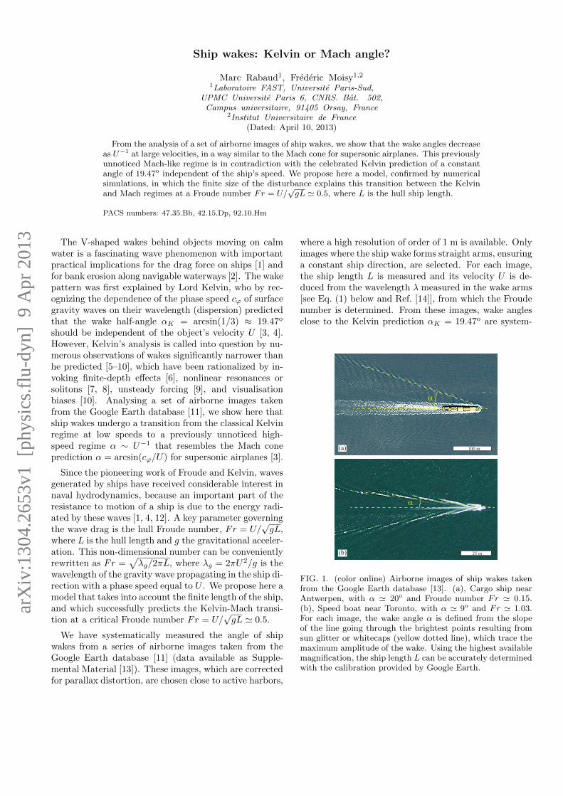
Ship wakes: Kelvin or Mach angle?

Marc Rabaud1, Frederic Moisy1,2

1Laboratoire FAST, Universite Paris-Sud,UPMC Universite Paris 6, CNRS. Bat. 502,

Campus universitaire, 91405 Orsay, France2Institut Universitaire de France

(Dated: April 10, 2013)

From the analysis of a set of airborne images of ship wakes, we show that the wake angles decreaseas U−1 at large velocities, in a way similar to the Mach cone for supersonic airplanes. This previouslyunnoticed Mach-like regime is in contradiction with the celebrated Kelvin prediction of a constantangle of 19.47o independent of the ship’s speed. We propose here a model, confirmed by numericalsimulations, in which the finite size of the disturbance explains this transition between the Kelvinand Mach regimes at a Froude number Fr = U/

√gL ' 0.5, where L is the hull ship length.

PACS numbers: 47.35.Bb, 42.15.Dp, 92.10.Hm

The V-shaped wakes behind objects moving on calmwater is a fascinating wave phenomenon with importantpractical implications for the drag force on ships [1] andfor bank erosion along navigable waterways [2]. The wakepattern was first explained by Lord Kelvin, who by rec-ognizing the dependence of the phase speed cϕ of surfacegravity waves on their wavelength (dispersion) predictedthat the wake half-angle αK = arcsin(1/3) ≈ 19.47o

should be independent of the object’s velocity U [3, 4].However, Kelvin’s analysis is called into question by nu-merous observations of wakes significantly narrower thanhe predicted [5–10], which have been rationalized by in-voking finite-depth effects [6], nonlinear resonances orsolitons [7, 8], unsteady forcing [9], and visualisationbiases [10]. Analysing a set of airborne images takenfrom the Google Earth database [11], we show here thatship wakes undergo a transition from the classical Kelvinregime at low speeds to a previously unnoticed high-speed regime α ∼ U−1 that resembles the Mach coneprediction α = arcsin(cϕ/U) for supersonic airplanes [3].

Since the pioneering work of Froude and Kelvin, wavesgenerated by ships have received considerable interest innaval hydrodynamics, because an important part of theresistance to motion of a ship is due to the energy radi-ated by these waves [1, 4, 12]. A key parameter governingthe wave drag is the hull Froude number, Fr = U/

√gL,

where L is the hull length and g the gravitational acceler-ation. This non-dimensional number can be convenientlyrewritten as Fr =

√λg/2πL, where λg = 2πU2/g is the

wavelength of the gravity wave propagating in the ship di-rection with a phase speed equal to U . We propose here amodel that takes into account the finite length of the ship,and which successfully predicts the Kelvin-Mach transi-tion at a critical Froude number Fr = U/

√gL ' 0.5.

We have systematically measured the angle of shipwakes from a series of airborne images taken from theGoogle Earth database [11] (data available as Supple-mental Material [13]). These images, which are correctedfor parallax distortion, are chosen close to active harbors,

where a high resolution of order of 1 m is available. Onlyimages where the ship wake forms straight arms, ensuringa constant ship direction, are selected. For each image,the ship length L is measured and its velocity U is de-duced from the wavelength λ measured in the wake arms[see Eq. (1) below and Ref. [14]], from which the Froudenumber is determined. From these images, wake anglesclose to the Kelvin prediction αK = 19.47o are system-

(a)

(b)

α

α

100 m

25 m

FIG. 1. (color online) Airborne images of ship wakes takenfrom the Google Earth database [13]. (a), Cargo ship nearAntwerpen, with α ' 20o and Froude number Fr ' 0.15.(b), Speed boat near Toronto, with α ' 9o and Fr ' 1.03.For each image, the wake angle α is defined from the slopeof the line going through the brightest points resulting fromsun glitter or whitecaps (yellow dotted line), which trace themaximum amplitude of the wake. Using the highest availablemagnification, the ship length L can be accurately determinedwith the calibration provided by Google Earth.

arX

iv:1

304.

2653

v1 [

phys

ics.

flu-

dyn]

9 A

pr 2

013

2

atically found at low Fr, i.e. for L � λg (Fig. 1a). Inthis case, a double wedge pattern, generated by the bowand the stern, can be observed. At larger Fr, λg reachesthe ship length L, resulting in interacting bow and sternwaves. At this point it is known that the trim of theboat is affected and the wave drag strongly increases:this is the so-called hull limit velocity [1, 4] — even ifpowerful speed boats or sailing boats nowadays overcomethis limit. At even larger Fr (L � λg), the hull partlyrises out of the water, entering in the so-called planingregime [1]. It is in this large-Fr regime that we find ex-amples of narrow wakes, with angles of 10o or less, asillustrated in Fig. 1b.

The wake angles measured from the airborne imagesare plotted as a function of the Froude number in Fig.2. In spite of a significant scatter, which can be mainlyascribed to the uncertainty in measuring the wavelengthλ, the data clearly shows a plateau at α ' 18.6o ± 1.8o

up to Fr ' 0.5± 0.1, in good agreement with the Kelvintheory. For larger Fr, this Kelvin regime is followed bya decrease of the angle down to values of order of 7o forthe fastest boats of our dataset [13]. Interestingly, likein the Mach cone problem, this decrease approximatelyfollows a law α ∼ 1/Fr.

In order to explain the transition in the wake an-gle, the starting assumption is to relate each wavenum-ber k emitted by the ship hull to a specific angle α(k).This k-dependent angle can be inferred from the lineardispersion relation for gravity waves in deep water [3],ω2 = gk, from which it follows that the group velocitycg = dω/dk of each wavenumber k is half its phase speed

cϕ = ω/k =√g/k. Since the wake is stationary in the

reference frame of the ship, the phase speed of each kmust be given by the ship velocity projected in the di-

0.1 0.2 0.4 0.6 1 2 33

4

6

810

20

40

Wak

e an

gle

α (d

eg.)

Hull Froude number, Fr

Model (3)Asympt. (4)ImagesSimul.

FIG. 2. (color online) Log-log plot of the wake angle α asa function of the hull Froude number Fr = U/

√gL. Red

circles: angles measured from the 37 airborne images of thedataset [13]. Blue line: model (3). Blue dotted line: asymp-totic law (4). Yellow squares: numerical simulations.

rection of the wave propagation,

U cos θ(k) = cϕ(k) =√g/k. (1)

Accordingly, only wavenumbers k ≥ kg = 2π/λg = g/U2

can form a stationary pattern. Following the geometricalconstruction of Ref. [15] (see Fig. 3), we consider a waveof given wavenumber k emitted at time −t in the direc-tion θ(k) given by Eq. (1) when the boat was in M, withMO= Ut. Since its group velocity is half its phase speed,the distance MH= cgt traveled by this wave is half thedistance MI= cϕt. It follows that the wedge angle formedby this particular wavenumber k is

α(k) = tan−1

√k/kg − 1

2k/kg − 1, (2)

which is plotted in Fig. 4. This angle vanishes at thelower bound k = kg allowed by the ship velocity (cor-responding to the transverse wave λg shown in Fig. 3)and at k → ∞, and reaches the maximum αK =tan−1(1/

√8) ' 19.47o at k = 3kg/2. No energy can be

found outside this wedge of angle αK , so if all wavenum-bers are excited (flat disturbance spectrum), the classicalKelvin angle αK is found.

An important point is that the departure from theKelvin angle αK in Fig. 2 is observed at large velocities,for which both viscosity and surface tension effects canbe neglected, so a model for the Kelvin-Mach transitionmust rely only on gravity waves. The key assumptionhere is that a ship of size L cannot excite waves of sizemuch larger than L, suggesting to model the finite size ofthe ship by a disturbance spectrum Ed(k) truncated atlow wavenumber. The simplest choice is a Heaviside stepspectrum, Ed(k) ∝ H(k−kL), with a cutoff wavenumberkL = 2π/L. The resulting wake angle is therefore simplygiven by the maximum of (2) taken over the range of ex-cited wavenumbers, [kL,∞[. When kL ≤ 3kg/2, i.e. for

M O

k

I

αθ

λ

Ut

cgt

cϕt

λg

H

FIG. 3. Wake angle α(k) of a given Fourier component k. Thewave of wavenumber k emitted in the direction θ(k) at time−t when the ship was in M reaches at time 0 the point H atthe middle of MI because the group velocity is half the phasespeed. The wave crests illustrate the transverse waves λg atα = 0 and the divergent waves λ at α 6= 0 (with λ = 2λg/3for the classical Kelvin wake).

3

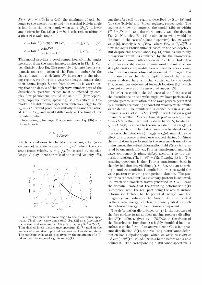
Fr ≤ Frc =√

3/4π ' 0.49, the maximum of α(k) be-longs to the excited range and the classical Kelvin angleis found; on the other hand, when kL > 3kg/2, a lowerangle given by Eq. (2) at k = kL is selected, resulting ina piecewise wake angle

α = tan−1(1/√

8) ' 19.47o, F r ≤ Frc (3a)

α = tan−1

√2πFr2 − 1

4πFr2 − 1, F r ≥ Frc, (3b)

This model provides a good comparison with the anglesmeasured from the wake images, as shown in Fig. 2. Val-ues slightly below Eq. (3b) probably originate from a sys-tematic underestimation of the Froude number for thefastest boats: at such large Fr boats are in the plan-ing regime, resulting in a waterline length smaller thantheir actual length L seen from above. It is worth not-ing that the details of the high wave-number part of thedisturbance spectrum, which must be affected by com-plex flow phenomena around the ship hull (flow separa-tion, capillary effects, splashing), is not critical in thismodel. All disturbance spectrum with no energy belowkL = 2π/L would produce essentially the same transitionat Fr = Frc, and would differ only in the limit of lowFroude number.

Interestingly, for large Froude numbers, Eq. (3b) sim-ply reduces to

α ≈ 1

2√

2πFr, (4)

which is analogous to the Mach cone angle for (non-dispersive) acoustic waves, α ' cg/U , where the con-

stant group velocity cg = 12

√g/kL selected by the ship

length L plays here the role of the sound velocity. We

10−1 10 0 10 1 10 20

5

10

15

20

25

30Fr = 0.25 0.5 1 2

- - - Ed (k) (arb. units)

k / kg

α(k

) (d

eg.)

FIG. 4. Selection of the wake angle by the disturbance spec-trum. Thick line: wake angle α(k) [Eq. (2)] as a function ofthe normalized wavenumber k/kg, with kg = g/U2 = 2π/λg.Thin dashed lines: disturbance spectrum Ed(k) used in thenumerical simulation, plotted for various Froude numbers.The resulting wake angle α is given by the maximum of α(k)taken over the range of significant Ed(k).

can therefore call the regimes described by Eq. (3a) and(3b) the ’Kelvin’ and ’Mach’ regimes, respectively. Theasymptotic law (4) matches the model (3b) to within1% for Fr > 1, and describes equally well the data inFig. 2. Note that Eq. (4) is similar to what would beobtained in the case of a (non-dispersive) shallow waterwake [6], namely α ≈ 1/FrH , where FrH = U/

√gH is

now the depth Froude number based on the sea depth H.But despite this resemblance, Eq. (4) remains essentiallya dispersive result, as confirmed by the the characteris-tic feathered wave pattern seen in Fig. 1(b). Indeed, anon-dispersive shallow-water wake would be made of twostraight crests comparable to a supersonic shock wave,which we have never observed in our set of images. Thefinite size rather than finite depth origin of the narrowwakes analysed here is further confirmed by the depthFroude number determined for each location [16], whichdoes not correlate to the measured angles [13].

In order to confirm the influence of the finite size ofthe disturbance on the wake angle, we have performed apseudo-spectral simulation of the wave pattern generatedby a disturbance moving at constant velocity with infinitewater depth. The simulation is carried out in a squaredomain r = (x, y) ∈ [−D/2, D/2]2, discretized on a gridof size N = 2048. At each time step δt = δx/U , whereδx = D/N is the mesh unit, a disturbance δζ located atrs = (D/4, 0) is added to the surface deformation ζ(r, t)initially set to 0. The disturbance is a localized defor-mation of the interface δζ = wd(r− rs)δt, mimicking theeffect of a pressure disturbance applied during δt. Sincethe simulation is performed in the reference frame of thedisturbance, the actual deformation field ζ(r, t) is trans-lated by one mesh unit δx, Fourier-transformed, and eachwave component is phase-shifted according to the dis-persion relation, ζ(k, t + δt) = ζ(k, t) exp[iω(k) δt]. Theresulting spectrum is then Fourier-transformed back inthe physical domain, yielding ζ(r, t+ δt), and an absorb-ing boundary condition is applied in order to avoid thewake pattern re-entering the periodic domain. The pro-cedure is repeated until a stationary pattern is achieved,i.e. when the transient waves generated at t = 0 leavethe domain. Note that the resulting deformation ζ(r)is complex, with the real part being the actual surfacedeformation (related to the potential energy), and theimaginary part coding for the phase of the wave (relatedto the kinetic energy, which is in phase quadrature withthe potential energy for each Fourier component).

The deformation disturbance wd(r) is the response ofthe free surface to an applied moving pressure distribu-tion P (r − Utex), given by −U∂P/∂x in the frame ofthe disturbance. Introducing a highly simplified hull dis-turbance in the form of an axisymmetric Gaussian pres-sure distribution P (r), the resulting disturbance defor-mation has a dipolar shape, which we write as wd(r) ∝−∂[exp(−2π2(r/L)2)]/∂x, with a bump before and a holebehind it. The corresponding disturbance spectrum is

4

Ed(k) = |wd(k)|2 ∝ k2x|P (k)|2 ∝ k2x exp[−(kL)2/4π2],which is maximum at kx = 2π/L. This model spectrum(plotted in Fig. 4 for four values of the Froude number)has therefore an effective low-wavenumber cutoff, whichis the fundamental ingredient of the Heaviside step spec-trum leading to the wake angle (3). Its decrease at large k(which is required for numerical convergence) should notaffect the wake angle selection, provided that the Froudenumber is not too small.

The simulated wake patterns shown in Fig. 5 for fourFroude numbers reproduce successfully the key featuresof the ship wake observations. Interestingly, at Fr = 0.5,the transverse wave of wavelength λg is clearly presentin the field, in addition to the divergent wave of wave-length 2λg/3 along the cusp line at α ' 19o, as com-monly observed behind boats at moderate Froude num-bers. Froude numbers below 0.3 produce no wake, be-cause the range of wavenumbers k ∈ [kg,∞[ is not signif-icantly fed by the disturbance spectrum (see the curve atFr = 0.25 in Fig. 4); this is a limitation of the smoothpressure distribution chosen here, which does not pos-sess the high-wavenumber energy content of the Heavi-side spectrum used in the model. At larger Fr, only thedivergent wave is present, since the transverse compo-nent at kg falls outside the disturbance spectrum Ed(k).We can note the broad wake arms at Fr = 1, for whichEd(k) covers a range where α(k) varies significantly. Atlarger Fr, Ed(k) picks only a narrow range of α(k), andthe wake angle becomes more precisely selected. The

(a) Fr = 0.5, α = 18.9° (b) Fr = 1, α = 15.9°

(c) Fr = 2, α = 5.8° (d) Fr = 4, α = 2.9°

FIG. 5. (color online) Wake pattern obtained from numericalsimulation, for Froude numbers Fr = 0.5, 1, 2 and 4. Thedisturbance size is L = 4 m, and the imaged domain is 140 m.The upper panel of each image shows the physical amplitudeR{ζ(x, y)}, and the lower panel shows the modulus |ζ(x, y)|.Wake angles (shown as yellow squares in Fig. 2) are measuredfrom best linear fit of the maximum of |ζ(x, y)|. Black dottedlines indicate the Kelvin angle αK = 19.47o.

wake angles have been measured from a linear fit throughthe maxima of the modulus of the complex deformation|ζ(x, y)| (shown in Fig. 5), which conveniently displaysthe square root of the total energy in the physical space.The resulting wake angles, also plotted in Fig. 2 (yellowsquares), are in good agreement with the two branches(3a) and (3b), confirming that the Kelvin-Mach transi-tion at Fr ' 0.5 is correctly captured by the finite sizeeffect of the disturbance.

Our results suggest that the departure from conven-tional Kelvin wakes reported in the literature can be at-tributed at least in part to the effect of the finite sizeof the disturbance. The Mach-like ship wakes describedhere provide an intriguing example of a seemingly non-dispersive wake pattern, similar to a supersonic shockwave, although keeping its specific feathered shape char-acteristic of a dispersive medium. We are now extend-ing this approach to smaller scales, e.g. for ducks or in-sects [17, 18], for which richer wake patterns are expectedfrom the interplay between the capillary cutoff and thefinite size of the moving body.

We acknowledge N. Pavloff, E. Raphael and G.Rousseaux for fruitful discussions, and J.P. Hulin andN. Ribe for their comments to the manuscript.

[1] R. Garrett The symmetry of sailing (Sheridan House Inc.,England, 1987).

[2] P.D. Osborne and E.H. Boak, J. Coastal Res. 15(2), 388(1999). B.O. Bauer et al., Port, Coastal, Ocean Eng.128(4), 152 (2002).

[3] J. Lighthill Waves in fluids (Cambridge University Press,Cambridge, England, 1978).

[4] O. Darrigol Worlds of Flow: A History of Hydrodynamicsfrom the Bernoullis to Prandtl (Oxford University, 2005).

[5] A.M. Reed and J.H. Milgram, Ann. Rev. Fluid Mech. 34,469 (2002).

[6] M.C. Fang, R.Y. Yang, and I.V. Shugan, J. Mech. 27, 71(2011).

[7] E.D. Brown et al, J. Fluid Mech. 204, 263 (1989).[8] Q. Zhu, Y. Liu, and D.K.P. Yue, J. Fluid Mech. 597, 171

(2008).[9] C.C. Mei and M. Naciri, Proc. R. Soc. Lond. A 432, 535

(1991).[10] W.H. Munk, P. Scully-Power, and F. Zachariasen, Proc.

R. Soc. Lond. A 412, 231 (1987).[11] Google Earth, http://earth.google.com[12] E. Raphael and P.-G. de Gennes, Phys. Rev. E 53 (4),

3448 (1996).[13] Supplemental Material available at URL xxx.[14] C. Aguiar and A. Souza, Phys. Educ. 44, 624 (2009).[15] F.S. Crawford, Am. J. Phys. 60, 782 (1992).[16] Local depths are available from the marine charts pro-

vided by Navionics S.p.A., http://www.navionics.com[17] M. Benzaquen, F. Chevy, and E. Raphael, EPL 96, 34003

(2011).[18] I. Carusotto and G. Rousseaux, arXiv:1202.3494v1

(2012).