Labor Market Reforms and Unemployment Dynamics1

Fabrice Murtin2 Jean-Marc Robin3

24th September 2013

1This paper is part of the “Return to Work” project lead by the OECD (2011) and super-vised by Giuseppe Nicoletti and Alain de Serres. We thank Romain Duval, Jorgen Elmeskov,Alexander Hijzen, John Martin, Dale Mortensen, Christopher Pissarides, Fabien Postel-Vinay,Stefano Scarpetta, Jean-Luc Schneider, Paul Swaim, as well as the participants at seminars runat the OECD, Bristol and Cyprus University for helpful comments and suggestions. This paperexpresses the opinions of the authors and does not necessarily reflect the official views of theOECD. Robin gratefully acknowledges financial support from the Economic and Social ResearchCouncil through the ESRC Centre for Microdata Methods and Practice grant RES-589-28-0001,and from the European Research Council (ERC) grant ERC-2010-AdG-269693-WASP.

2fabrice.murtin@oecd.org, OECD3jeanmarc.robin@sciences-po.fr, Sciences-Po and University College London

Abstract

In this paper, we quantify the contribution of labor market reforms to unemployment

dynamics in nine OECD countries (Australia, France, Germany, Japan, Portugal, Spain,

Sweden, the United Kingdom and the United States). We build and estimate a dynamic

stochastic search-matching model with heterogeneous workers, where aggregate shocks to

productivity fuel up the cycle, and unanticipated policy interventions shift structural pa-

rameters and displace the long-term equilibrium. We show that the heterogeneous-worker

mechanism proposed by Robin (2011) to explain unemployment volatility by productivity

shocks works well in all countries. We find that placement and employment services is

the most important determinant of structural unemployment change.

JEL classification: E24, E32, J21.

Keywords: Unemployment dynamics, turnover, labor market institutions, job search,

matching function.

1 Introduction

A large number of studies have sought the source of persistent differences in European

and American labor market outcomes in different labor market institutions. Following

Bruno and Sachs (1985), research hunted down the most effective labor market policies

by running pooled cross-country time-series regressions of unemployment rates on various

macroeconomic indicators (like GDP growth) and a battery of labor market institutional

indices (see Nickell and Layard, 1999, for a survey). Blanchard and Wolfers (2000) and

Bertola, Blau and Khan (2007) thus showed that different policy mixes induced different

responses of unemployment to world-wide shocks (like an oil shock) and country-specific

productivity shocks, and more recently, Bassanini and Duval (2009) emphasized the ex-

istence of complementarities between labor market policies. In parallel, in order to un-

derstand the mechanisms of these interactions, research spawned a collection of small

dynamic stochastic equilibrium models focussing on one particular labor market policy at

a time. For example, the influential work of Ljungqvist and Sargent (1998) emphasized

the link between long-term unemployment and welfare policies, while Prescott (2004) and

Rogerson (2008) more recently emphasized the role of labor taxes.

In this paper we will try to incorporate the rich reduced forms of the former approach

into a small equilibrium model of the latter kind. The idea is to identify a small set of

parameters of the dynamic equilibrium model governing the responses to aggregate shocks

of unemployment and turnover, and channelling a wide range of labor market policies at

the same time. The number of policies simultaneously examined can be large but the

number of parameters through which they impact the economy should be kept small,

because, for the model to be identified, the number of intervention channels should be

less than the number of independent series used in the analysis. Specifically, if we use

series of unemployment stocks and flows, and vacancies, as labor market variables, we

argue that it will be difficult to identify more than three separate channels for policy

intervention.1

1The change in unemployment is the difference between the inflow and the outflow. So stocks andflows are not independent series.

1

We develop a dynamic stochastic search-matching model with heterogeneous workers,

where aggregate shocks to productivity fuel up the cycle, and unanticipated policy inter-

ventions displace the stationary stochastic equilibrium by shifting structural turnover pa-

rameters. It is estimated in nine different countries (Australia, France, Germany, Japan,

Portugal, Spain, Sweden, the United Kingdom and the United States) over the period

1985-2007 using the following two-step procedure. First, a version without policy inter-

ventions is estimated with detrended series by the Simulated Method of Moments, and

aggregate shocks are filtered out by minimizing the sum of squared differences between

actual and simulated aggregate output series. Second, policy effects are introduced into

the model, and estimated by minimizing the sum of squared residuals for the series of

actual unemployment rates (i.e. trend plus cycle), unemployment flows and job vacancies.

The model builds on Mortensen and Pissarides (1994, henceforth MP). Yet, it is im-

mune to Shimer’s (2005) critique. Shimer showed that in the MP model Nash bargaining

converts most of the cyclical volatility of aggregate productivity into wage volatility, leav-

ing little room for change to the key variable driving unemployment, market tightness.

In the same issue, Hall (2005) presented a calibration showing that the unemployment

volatility puzzle could indeed be solved by wage rigidity.2 However, his argument was re-

cently contested by Pissarides (2009), who presented empirical evidence that the volatility

of wages in new jobs, those that proceed from vacancies, is large compared to the volatility

of ongoing wages. Finally, it is important to mention Hagedorn and Manovskii’s (2008)

solution to the puzzle, which also does not require wage rigidity. However, it is a rather

unrealistic calibration of the MP model with a very large value of non market time.

Our model extends the model of Robin (2011) by endogenizing labor demand through a

matching function and vacancy creation. It has two main ingredients that make it distinct

from the MP model, namely heterogenous worker abilities3 and a different wage setting

mechanism. First, workers differ in ability. In good states of the economy, all matches are

profitable and all workers are employable. In bad states, low-skill workers fail to generate2See also Hall and Milgrom (2008) and Gertler and Trigari (2009).3In this simple version of the model, we abstract from firm heterogeneity in production. For an

extension of the model with heterogeneous firms, see Lise and Robin (2013).

2

positive surplus and are thus laid off or stay unemployed longer. With a thick left tail

of the ability distribution, small adverse shocks to the economy lead a disproportionately

high number of low-skill workers into the negative surplus region and into unemployment.

We show that this amplification mechanism fits unemployment volatility well in all nine

major OECD countries used in the empirical analysis.

We also assume that wage contracts are long term contracts that can only be rene-

gotiated by mutual agreement (see Postel-Vinay and Robin, 2002). Wage renegotiation

is either induced by on-the-job search and Bertrand competition between employers, or

by aggregate shocks big enough to threaten match disruption. As a consequence, wages

in new jobs are more volatile than ongoing wages.4 This assumption also tremendously

simplifies the form of the Bellman equation defining the surplus of a match with a worker

of a given type in a given state of the economy, and it thus makes the dynamic stochastic

equilibrium very easy to solve.

Ultimately, we use our model to assess the impact of labor market reforms on the actual

(i.e. not detrended) rate of unemployment by way of counterfactual simulation. We find

over the period 1985-2007 a significant effect of active labor market policies — especially

placement and employment services, nearly a full percentage point of unemployment. All

other policies have a more limited impact, between a fifth and a third of a percentage

point.

The paper is organized as follows. In Section 2, a dynamic sequential-auction model

with heterogeneous workers and identical firms is developed. Section 3 describes the data

and Section 4 the estimation procedure. In Section 5, the business cycle version of the

model is estimated on nine OECD countries. In Section 6, labor market policy effects are

estimated. The last section concludes.4Hall and Krueger (2012) emphasize the empirical relevance of on-the-job search to explain wage

formation.

3

2 The model

Time is discrete and indexed by t ∈ N. The global state of the economy is an ergodic

Markov chain yt ∈ {y1 < ... < yN} with transition matrix Π = (πij). We use yt to denote

the random variable and yi or yj to denote one of the N possible realizations. There are

M types of workers and `m workers of each type, with `1 + ...+ `M = 1. Workers of type

m have ability xm and xm < xm+1. All firms are identical. Workers and firm are paired

into productive units. The per-period output of a worker of ability xm when aggregate

productivity is yi is denoted as yi(m).

2.1 Turnover and unemployment

Matches form and break at the beginning of each period. Let ut(m) denote the proportion

of unemployed in the population of workers of ability xm at the end of period t − 1, or

at the beginning of period t, just before revelation of the aggregate shock for period t,

and let ut = ut(1)`1 + ...+ ut(M)`M define the aggregate unemployment rate. Let St(m)

denote the surplus of a match with a worker of type xm at time t, that is, the present

value of the match minus the value of unemployment and minus the value of a vacancy

(assumed to be nil). Only matches with positive surplus St(m) ≥ 0 are viable.

At the beginning of period t, yt is realized and a new value St(m) is observed for

the match surplus. An endogenous fraction 1{St(m) < 0}[1 − ut(m)]`m of employed

workers is immediately laid off if the match surplus becomes negative, and another fraction

δ1{St(m) ≥ 0}[1− ut(m)]`m is otherwise destroyed. In addition, a fraction λt1{St(m) ≥

0}ut(m)`m of employable unemployed workers meet with a vacancy. Finally, we also allow

employees to meet with alternative employers, and move or negotiate wage increases (more

on this later).

Aggregate shocks thus determine unemployment by conditioning job destruction and

the duration of unemployment. The law of motion for individual-specific unemployment

4

rates is

ut+1(m) =

1 if St(m) < 0,

ut(m) + δ(1− ut(m))− λtut(m) if St(m) ≥ 0.

The dynamics of unemployment by worker type depends on the dynamics of the whole

match surplus, not on how the surplus is split between the employer and the worker.

Define the exit rate from unemployment (or job finding rate) as the product of the

meeting rate and the share of employable unemployed workers,

ft = λt

∑m ut(m)`m1{St(m) ≥ 0}

ut. (1)

Define also the job destruction rate as the sum of the exogenous and the endogenous layoff

rates,

st = δ + (1− δ)∑

m(1− ut(m))`m1{St(m) < 0}1− ut

. (2)

Aggregate unemployment then satisfies the usual recursion:

ut+1 = ut + st(1− ut)− ftut.

It is important to stress here that both the job finding rate ft and the job destruction

rate st mix structural parameters (in λt and δ) with endogenous variables: the share

of employable unemployed workers (∑

m 1{St(m)≥0}ut(m)`mut

) and the share of unemployable

employed workers (∑

m 1{St(m)<0}(1−ut(m))`m1−ut ). For that reason, standard least-squares es-

timates of matching functions or layoff rates will not provide consistent estimators. A

structural estimation is required.

2.2 Rent sharing

We assume that employers have full monopsony power with respect to unemployed work-

ers. They keep the whole surplus in this case and unemployed workers leave unemployment

with a wage that is only marginally greater than their reservation wage. The assump-

5

tion that unemployed workers have zero bargaining power relative to employers is mainly

technical: it makes the dynamics of unemployment independent of wages. As the focus

of this paper is on unemployment dynamics and worker flows, we believe that this decou-

pling is justified. Note however that we could easily allow for Nash bargaining between

unemployed workers and firms, but this would complicate the model a lot for a very small

gain.

Employed workers search on the job. When the search for an alternative employer is

successful, we assume that Bertrand competition between the incumbent and the poacher

transfers the entire surplus to the worker. The worker is indifferent between staying or

moving. We assume that job-to-job mobility is then decided by coin tossing. Employer

heterogeneity would eliminate this indeterminacy, at the cost of great additional complex-

ity (Lise and Robin, 2013).

2.3 Vacancy creation and market tightness

Firms post vacancies vt until ex ante profits are exhausted. The total vacancy cost is cvt.

Vacancies can either randomly meet with an unemployed worker or with an employed

worker.5 However, only the meetings with unemployed workers generate a profit to the

firm. Free entry then ensures that

cvt = λt

M∑m=1

ut(m)`mSt(m)+, (3)

where we denote x+ = max(x, 0).

Define market tightness as the ratio of vacancies and workers’ aggregate search inten-

sity,

θt =vt

ut + k(1− ut), (4)

where k is the relative search intensity of employees with respect to unemployed.6 The5We assume that firms cannot direct search towards specific workers (the unemployed), as this fea-

ture would bring the model too close from a competitive labor market, which is unlikely to be verifiedempirically.

6We use k = 0.12 as in Robin (2011) but imposing a zero search intensity for employees has littleinfluence on the estimation outcome.

6

meeting rate λt is related to market tightness via the meeting function, λt = f(θt), where

f is an increasing function, likely concave.

2.4 The value of unemployment and the match surplus

Let Ui(m) denote the present value of remaining unemployed for the rest of period t for

a worker of type m if the economy is in state i. It solves the following linear Bellman

equation:

Ui(m) = zi(m) +1

1 + r

∑j

πijUj(m). (5)

This equation is understood as follows. An unemployed worker receives a flow-payment

zi(m) for the period. At the beginning of the next period, the state of the economy changes

to yj with probability πij and the worker receives a job offer with some probability. We

have assumed that employers offer unemployed workers their reservation wage on a take-

it-or-leave basis, thus effectively reaping the whole surplus. As a consequence, the present

value of a new job to the worker is only marginally better than the value of unemployment.

Hence, the continuation value is the value of unemployment in the new state j whether

the workers remains unemployed or not.

Let us now turn to the match surplus. After a productivity shock from i to j all

matches yielding negative surplus are destroyed. Then, either on-the-job search delivers

no bite, and the match surplus only changes because the macroeconomic environment

changes; or the worker is poached and Bertrand competition gives the whole match surplus

to the worker, whether she moves or not. As everything that the worker expects to earn

in the future contributes to the definition of the current surplus, the surplus of a match

with a worker of type m when the economy is in state i thus solves the following (almost

linear) Bellman equation:

Si(m) = yi(m)− zi(m) +1− δ1 + r

∑j

πijSj(m)+. (6)

This almost-linear system of equations can be solved numerically by value function itera-

tion. As for the unemployment value, the match surplus only depends on the state of the

7

economy.

2.5 Steady-state equilibrium

If the economy stays in state i for ever, the equilibrium unemployment rate for group m

is

ui(m) =δ

δ + λi1{Si(m) ≥ 0}+ 1{Si(m) < 0} = 1− λi

δ + λi1{Si(m) ≥ 0},

where λi ≡ f(θi). The aggregate unemployment rate is

ui =M∑m=1

ui(m)`m = 1− λiδ + λi

Li,

where Li =∑M

m=1 `m1{Si(m) ≥ 0} is the number of employable workers. Lastly, the free

entry condition takes the following form:

cθi = λi

M∑m=1

ui(m)`mui + k(1− ui)

Si(m)+ =δλi

δ + [1− Li + k(1− δ)Li]λiS+

i ,

with S+

i =∑M

m=1 `mSi(m)+ being the aggregate surplus value. Therefore, the exit rate

from unemployment is the following fixed point:

λi = f

(δλi

δ + [1− Li + k(1− δ)Li]λiS+

i

c

).

The steady-state equilibrium is thus characterized as a fixed point of a simple nonlinear

function that can be solved by iterating the function.

2.6 Parameterization and functional forms

Unemployment exit rate and the matching function. The meeting rate, and

hence the unemployment exit rate, are related to market tightness θt via a Cobb-Douglas

matching technology:

λt = f(θ) = φθη. (7)

8

A standard cross-country OLS regression of job finding rates on tightness (in logs) simply

defined as v/u delivers estimates of matching efficiency φ = 0.712 and matching elasticity

η = 0.289, in tune with the empirical literature (Murrain and de Serres, 2013).

Aggregate shocks. We assume that aggregate productivity follows a Gaussian AR(1)

process:

ln yt = ρ ln yt−1 + σεt, (8)

where innovations are iid-normal N(0, 1). Note that the aggregate productivity shock yt

is a latent process that does not a priori coincide with observed output or output per

worker. Indeed, observed output is the aggregation of match output yt(m) across all

active matches, say

Yt =∑m

[1− ut(m)] `m yt(m), (9)

and is thus endogenous. Therefore, the structural parameters (ρ, σ) cannot be directly

inferred from the observed series of aggregate output.

We discreetness the aggregate productivity process yt as follows. Let F denote the

estimated equilibrium distribution of yt.7 The joint distribution of two consecutive ranks

F (yt) and F (yt+1) is a copula C (i.e. the CDF of the distribution of two random variables

with uniform margins). To discreetness the aggregate productivity processes we first

specify a grid a1 < ... < aN on [ε, 1 − ε] ⊂ (0, 1) of N linearly spaced points including

end points ε and 1− ε. Then we set yi = F−1(ai) and πij ∝ c(ai; aj), where c denotes the

copula density and we impose the normalization∑

j πij = 1. In practice, we use N = 150,

ε = 0, 002; F is a log-normal CDF and c is a Gaussian copula density, as implied by the

Gaussian AR(1) specification.

Worker heterogeneity. Match productivity is specified as yi(m) = yixm, where (xm,m =

1, ...,M) is a grid of M linearly spaced points on the interval [C,C + 1]. The choice of

the support does not matter much provided that it is large enough and contains one. A

7That is, with white-noise innovations, ln yt ∼ N(0, σ2

1−ρ2

).

9

beta distribution is assumed for the ability distribution, namely

`m ∝ betapdf (xm, ν, µ) , (10)

with the normalization∑

m `m = 1. The beta distribution allows for a variety of shapes

for the density (increasing, decreasing, non monotone, concave or convex). We use a very

dense grid of M = 500 points to guarantee a good resolution in the left tail.

Leisure and vacancy costs. The opportunity cost of employment zi(m) (aggregating

the utility of leisure, unemployment insurance and welfare) is specified as a constant z.

Labor market institutions. Because of the feed-back effects implied by the model, it

is important for identification that we restrict the channels of policy interventions. For

example, any policy that directly impacts matching efficiency (φ) immediately changes

the meeting rate (λt) and, subsequently, the number of created vacancies (vt) via the

free entry condition. Both effects contribute to changing the job finding rate (ft). If one

makes the cost of posting a vacancy (c) a concurrent intervention channel for this policy,

then the policy affects vacancy creation in two ways, which evidently reduces the chances

that the model be identified.

Because we only have independent data information on turnover flows (ft and st) and

vacancies (vt) we decided to introduce labor market policies (henceforth LMPs) through

only three structural parameters: matching efficiency (φ) via equation (1), the job de-

struction rate (δ) via equation (2), and the cost of posting a vacancy (c) via equation

(3). Formally, we let parameters φ, δ and c in country n at time t be log-linear indices of

country-specific institutional variables X1nt, ..., X

Knt:

φnt = φ0n exp

(∑k

φkXknt

), δnt = δ0n exp

(∑k

δkXknt

), cnt = c0n exp

(∑k

ckXknt

).

In these equations, the LMP semi-elasticities (φk, δk, ck) are common to all countries.

However, intercepts (φ0n, δ

0n, c

0n) are country-specific. This framework thus identifies insti-

tutional effects from policy variations.

10

Table 1: Unemployment and Turnover Cycle - Descriptive Statistics

Period Unemployment Job Destruction Rate Job Finding Ratemean std std mean std mean std

trend cycle trend cycle trend cycleAustralia 1979Q1-2009Q4 5.69 2.62 1.19 1.10 3.78 0.36 0.23 47.74 6.62 5.69Germany 1984Q1-2010Q1 6.09 2.72 1.27 1.06 1.81 0.06 0.52 18.71 0.88 2.71Spain 1978Q1-2010Q2 12.76 4.10 1.94 2.78 3.88 0.73 0.16 21.67 8.04 5.55France 1976Q1-2010Q1 6.18 3.33 1.58 0.77 2.41 0.43 0.16 22.59 3.64 2.78UK 1967Q2-2010Q1 6.25 2.74 1.86 1.29 3.06 0.48 0.60 43.87 15.22 5.35Japan 1978Q1-2007Q4 2.65 1.31 0.92 0.49 1.51 0.27 0.22 42.78 4.21 4.83Portugal 1987Q1-2010Q2 5.70 2.29 0.84 1.22 1.45 0.20 0.42 20.58 0.99 3.55Sweden 1972Q1-2010Q1 4.81 3.03 2.20 1.85 2.84 0.75 0.27 56.06 10.14 6.31US 1960Q1-2010Q2 5.95 1.54 0.75 1.14 4.82 0.68 0.66 76.59 6.03 5.21

Notes: All figures are in percent. Series were detrended using the HP-filter with smoothing parameter105.

3 The data

We have assembled data on labor market outcomes and institutions for nine OECD coun-

tries: Australia, France, Germany, Japan, Portugal, Spain, Sweden, United Kingdom and

Unites States, over the period 1985-2007. These data and their sources are described in

detail in Appendix A.

3.1 Unemployment and turnover cycle

Table 1 provides descriptive statistics on the rate of unemployment as well as the probabil-

ity of entering and exiting unemployment. All series are quarterly. The trend and cyclical

components were extracted by HP-filtering the log-transformed series with a smoothing

parameter equal to 105, as in Shimer (2005), and re-exponentiating. The volatility of

unemployment and of turnover are very different across countries. Japan displays lower

and less volatile unemployment, due to lower job destruction rates, than any other coun-

try. The US exhibit more turnover and higher exit rates from unemployment. France,

and Japan to a lesser extent, display particularly low cyclical volatility in unemployment

turnover.

Interesting patterns emerge from trends (Figure 1). Unemployment culminates in the

1980s in the UK and the US, and in the 1990s in Australia, France, Spain and Sweden.

11

−2

02

46

81960 1970 1980 1990 2000 2010

time

AUS

−2

02

46

8

1960 1970 1980 1990 2000 2010

time

DEU

−5

05

10

15

1960 1970 1980 1990 2000 2010

time

ESP

−5

05

10

1960 1970 1980 1990 2000 2010

time

FRA

−5

05

10

1960 1970 1980 1990 2000 2010

time

GBR

−2

02

46

1960 1970 1980 1990 2000 2010

time

JPN

−5

05

10

1960 1970 1980 1990 2000 2010

time

PRT

−5

05

10

1960 1970 1980 1990 2000 2010

time

SWE

−2

02

46

8

1960 1970 1980 1990 2000 2010

time

USA

(a) Unemployment

0.5

1

1960 1970 1980 1990 2000 2010

time

AUS

−.1

0.1

.2

1960 1970 1980 1990 2000 2010

time

DEU

−.2

0.2

.4

1960 1970 1980 1990 2000 2010

time

ESP

0.2

.4

1960 1970 1980 1990 2000 2010

time

FRA

0.5

1

1960 1970 1980 1990 2000 2010

time

GBR

0.2

.4.6

1960 1970 1980 1990 2000 2010

time

JPN

−.1

0.1

.2

1960 1970 1980 1990 2000 2010

time

PRT

0.5

1

1960 1970 1980 1990 2000 2010

time

SWE

0.5

1

1960 1970 1980 1990 2000 2010

time

USA

(b) Job Finding Rate

0.0

2.0

4

1960 1970 1980 1990 2000 2010

time

AUS

0.0

1.0

2

1960 1970 1980 1990 2000 2010

time

DEU

0.0

5.1

1960 1970 1980 1990 2000 2010

time

ESP

0.0

2.0

4

1960 1970 1980 1990 2000 2010

time

FRA

0.0

2.0

4

1960 1970 1980 1990 2000 2010

time

GBR

0.0

1.0

2

1960 1970 1980 1990 2000 2010

time

JPN

−.0

10

.01

.02

1960 1970 1980 1990 2000 2010

time

PRT

−.0

20

.02

.04

1960 1970 1980 1990 2000 2010

time

SWE

0.0

5.1

1960 1970 1980 1990 2000 2010

time

USA

(c) Job Destruction Rate

Figure 1: Unemployment Rate and Turnover - Trends and Cycles

12

Japan displays a monotonic, increasing trend throughout the 1960-2010 period. Unem-

ployment rebounds in the early 2000s in Portugal and the US. Long-term unemployment

trends hide strikingly different trends in turnover rates. Job destruction rates tend to

increase in France, Japan, Portugal, Spain and Sweden, and to decrease in Australia,

the UK and the US since the mid-1980s. Job-finding rates tend to increase in Australia,

France and Spain, and to decrease in Japan, Sweden, the UK and the US. These pat-

terns are potentially associated with important labor market reforms that we now briefly

discuss.

3.2 Labor market policies

The set of labor market policy variables used as potential determinants of unemployment

stocks and flows in the empirical analysis are the following: i) the replacement rate used

to calculate unemployment insurance (UI) benefits at first date of reception; ii) public ex-

penditure on active labor market policies per unemployed worker (ALMPs) normalized by

GDP per worker, and broken down into three sub-categories (placement and employment

services, employment incentives8 and training); iii) the OECD index of product market

regulation; iv) the OECD index of employment protection for regular contracts; v) the

tax wedge (personal income tax plus payroll taxes and social security contributions). We

exclude from the analysis LMPs such as the legal minimum wage, union density and other

wage bargaining institutions as they mostly affect wages, which are outside the scope of

this paper.

Table 2 displays the means and the standard deviations of all policy variables and their

year-on-year changes between 1985 and 2007 (the period over which we have gathered a

balanced sample of institutional variables). France, Portugal, Spain and Sweden offer

relatively high support to the unemployed and high employment protection at the same

time, whereas the US, the UK, Australia and Canada are on the low side. Germany

and Japan are somewhere in-between. Note that some institutions show no change in the

period (such as employment protection in the US). The associated policy effects cannot be8These expenditures include incentives to private employment, direct job creation, job sharing and

start-up incentives.

13

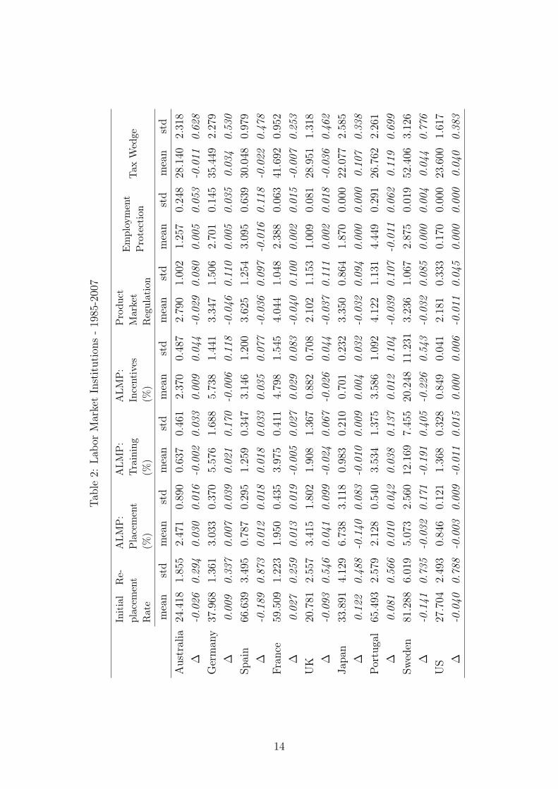
Table2:

Labo

rMarketInstitutions

-19

85-200

7

Initial

Re-

placem

ent

Rate

ALM

P:

Placement

(%)

ALM

P:

Training

(%)

ALM

P:

Incentives

(%)

Produ

ctMarket

Regulation

Employment

Protection

Tax

Wed

ge

mean

std

mean

std

mean

std

mean

std

mean

std

mean

std

mean

std

Australia

24.418

1.85

52.471

0.89

00.63

70.46

12.37

00.487

2.79

01.00

21.25

70.24

828

.140

2.31

8∆

-0.0

260.

294

0.03

00.

016

-0.0

020.

033

0.00

90.

044

-0.0

290.

080

0.00

50.

053

-0.0

110.

628

German

y37

.968

1.36

13.03

30.37

05.57

61.68

85.73

81.44

13.34

71.50

62.70

10.145

35.449

2.279

∆0.

009

0.33

70.

007

0.03

90.

021

0.17

0-0

.006

0.11

8-0

.046

0.11

00.

005

0.03

50.

034

0.53

0Sp

ain

66.639

3.49

50.78

70.29

51.25

90.34

73.146

1.20

03.62

51.25

43.09

50.63

930

.048

0.97

9∆

-0.1

890.

873

0.01

20.

018

0.01

80.

033

0.03

50.

077

-0.0

360.

097

-0.0

160.

118

-0.0

220.

478

Fran

ce59

.509

1.22

31.95

00.43

53.97

50.41

14.79

81.54

54.044

1.04

82.38

80.06

341

.692

0.95

2∆

0.02

70.

259

0.01

30.

019

-0.0

050.

027

0.02

90.

083

-0.0

400.

100

0.00

20.

015

-0.0

070.

253

UK

20.781

2.55

73.41

51.80

21.90

81.36

70.882

0.70

82.10

21.15

31.00

90.08

128

.951

1.31

8∆

-0.0

930.

546

0.04

10.

099

-0.0

240.

067

-0.0

260.

044

-0.0

370.

111

0.00

20.

018

-0.0

360.

462

Japa

n33

.891

4.12

96.73

83.11

80.98

30.21

00.70

10.23

23.35

00.86

41.870

0.00

022

.077

2.58

5∆

0.12

20.

488

-0.1

400.

083

-0.0

100.

009

0.00

40.

032

-0.0

320.

094

0.00

00.

000

0.10

70.

338

Portuga

l65

.493

2.57

92.12

80.54

03.53

41.375

3.58

61.09

24.12

21.13

14.44

90.29

126

.762

2.26

1∆

0.08

10.

566

0.01

00.

042

0.03

80.

137

0.01

20.

104

-0.0

390.

107

-0.0

110.

062

0.11

90.

699

Sweden

81.288

6.01

95.07

32.56

012.169

7.45

520.248

11.231

3.23

61.06

72.87

50.01

952

.406

3.12

6∆

-0.1

410.

735

-0.0

320.

171

-0.1

910.

405

-0.2

260.

543

-0.0

320.

085

0.00

00.

004

0.04

40.

776

US

27.704

2.49

30.84

60.12

11.36

80.328

0.84

90.04

12.18

10.33

30.17

00.00

023

.600

1.61

7∆

-0.0

400.

788

-0.0

030.

009

-0.0

110.

015

0.00

00.

006

-0.0

110.

045

0.00

00.

000

0.04

00.

383

14

Table 3: Labor Market Institutions - Correlated Change in 1985-2007

(1) (2) (3) (4) (5) (6) (7)(1) Initial Replacement Rate 1.000(2) ALMP: Placement -0.042 1.000(3) ALMP: Training 0.568 0.488 1.000(4) ALMP: Incentives 0.557 0.572 0.944 1.000(5) Product Market Regulation 0.224 0.046 0.409 0.303 1.000(6) Employment Protection 0.196 0.067 -0.077 -0.049 0.170 1.000(7) Tax Wedge 0.047 -0.451 -0.356 -0.391 -0.393 0.037 1.000Note: Correlations of deviations of LMPs from country-specific means.

identified in this case. The sign of the average policy change and its standard deviation,

identify the countries which intervened on this institutional front during the period. Only

product market regulation shows a convergence toward deregulation in all countries, and

only Portugal and Spain did reduce employment protection. All other policies show great

diversity across country. Finally, Sweden stands alone in its effort to reduce ALMP

spendings; but it true that it started from a very high point.

Table 3 displays the correlations between the LMP variables centered around their

country-specific means. The three ALMP components are strongly correlated, in particu-

lar training and firm incentives. Interestingly, any increase in product market regulation

or unemployment insurance is often accompanied by another policy aiming at reducing

the social cost of unemployment (more is spent on training or employment incentives or

in a reduction of the tax wedge). This is much less the case for employment protection.

As already emphasized, it is important for identification to restrict the channels of

policy interventions. Heuristically, in absence of a more formal model of the mechanisms

of policy interventions, we ended up restricting the mapping between LMPs and structural

parameters in the following way.

A first set of policies affect the search-matching technology. More generous unemploy-

ment benefits should reduce unemployed workers’ search intensity. More placement and

employment services should increase the rate at which unemployed workers find jobs, and

they should help improving match quality. Matches of higher quality should in turn be

more resilient to exogenous destruction shocks. More training provided to unemployed

15

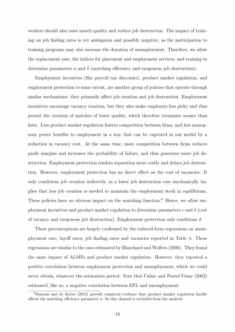
workers should also raise match quality and reduce job destruction. The impact of train-

ing on job finding rates is yet ambiguous and possibly negative, as the participation to

training programs may also increase the duration of unemployment. Therefore, we allow

the replacement rate, the indices for placement and employment services, and training to

determine parameters φ and δ (matching efficiency and exogenous job destruction).

Employment incentives (like payroll tax discounts), product market regulation, and

employment protection to some extent, are another group of policies that operate through

similar mechanisms: they primarily affect job creation and job destruction. Employment

incentives encourage vacancy creation, but they also make employers less picky and thus

permit the creation of matches of lower quality, which therefore terminate sooner than

later. Less product market regulation fosters competition between firms, and less monop-

sony power benefits to employment in a way that can be captured in our model by a

reduction in vacancy cost. At the same time, more competition between firms reduces

profit margins and increases the probability of failure, and thus generates more job de-

struction. Employment protection renders separation more costly and delays job destruc-

tion. However, employment protection has no direct effect on the cost of vacancies. It

only conditions job creation indirectly, as a lower job destruction rate mechanically im-

plies that less job creation is needed to maintain the employment stock in equilibrium.

These policies have no obvious impact on the matching function.9 Hence, we allow em-

ployment incentives and product market regulation to determine parameters c and δ (cost

of vacancy and exogenous job destruction). Employment protection only conditions δ.

These preconceptions are largely confirmed by the reduced-form regressions on unem-

ployment rate, layoff rates, job finding rates and vacancies reported in Table 4. These

regressions are similar to the ones estimated by Blanchard andWolfers (2000). They found

the same impact of ALMPs and product market regulation. However, they reported a

positive correlation between employment protection and unemployment, which we could

never obtain, whatever the estimation period. Note that Cahuc and Postel-Vinay (2002)

estimated, like us, a negative correlation between EPL and unemployment.9Murrain and de Serres (2013) provide empirical evidence that product market regulation hardly

affects the matching efficiency parameter φ. So this channel is excluded from the analysis.

16

Table 4: Reduced-form Regressions of Unemployment, Turnover and Tightness on LMPs

Log UNR Log LDR Log JFR Log V Log TightnessInitial Replacement Rate 0.064 0.030 -0.037 -0.065 -0.133

(0.008) (0.008) (0.008) (0.020) (0.021)ALMP: Placement -0.095 -0.069 0.020 -0.012 0.080

(0.006) (0.006) (0.006) (0.015) (0.016)ALMP: Training -0.126 -0.091 -0.014 -0.198 -0.099

(0.016) (0.015) (0.016) (0.042) (0.044)ALMP: Incentives 0.013 0.034 0.063 0.326 0.341

(0.016) (0.016) (0.017) (0.044) (0.046)Product Market Regulation 0.045 -0.016 -0.076 -0.167 -0.199

(0.011) (0.011) (0.011) (0.028) (0.030)Employment Protection -0.047 -0.078 -0.042 -0.006 0.046

(0.006) (0.006) (0.006) (0.015) (0.016)Tax Wedge 0.082 0.037 -0.051 0.015 -0.064

(0.007) (0.007) (0.007) (0.018) (0.019)

Notes: 1) All regressions contain country fixed effects and country-specific controls for business cycle (iethe HP-filtered log GDP). 2) Italicized estimates are not significant at the 5% level. 3) UNR:Unemployment Rate; LDR: Layoff rate; JFR: Job Finding Rate; V: Vacancies; Tightness =vacancies/unemployment.

The set of labor market policies is complemented by a handful of socio-demographic

variables, namely the shares of workers aged 15-24 and 55-64 in the 15-64 population, and

mean years of higher education among the 15-64 population. Indeed there is empirical

evidence (e.g. Murrain et al., 2013) that both unemployment entry and exit rates decline

with age. These socio-demographic variables are assumed to have an impact on turnover

parameters φ and δ.

4 Estimation procedure

The estimation is conducted in two steps. In the first step, we estimate a stationary version

of the model that fits the cyclical components of the series of GDP, unemployment, job

finding and job destruction rates, and vacancies separately for the nine OECD countries.

Then, we use the estimated model to filter out the series of aggregate shocks yt driving the

business cycle. In the second step, we introduce LMPs into the empirical framework and

we estimate their impact on the structural parameters φ, δ and c by fitting the raw series

17

(non detrended) of unemployment, turnover and vacancies jointly for all nine countries.

This estimation procedure is considerably easier to implement than any other method,

Bayesian or frequentist, for nonlinear state-space models.

4.1 Assessing business-cycle dynamics

The estimation of the parameters controlling for the short-term response of the economy

to business cycle shocks closely follows the method in Robin (2011). We assume that

HP-filtered series follow the model of this paper as in a stationary environment exempt

from any institutional change. Hence, we impose φk = δk = ck = 0 to each policy variable

(k ≥ 1) and each country. Ten parameters remain to be estimated: the country-specific

vacancy creation cost c0, the exogenous layoff rate δ0, the two parameters of the matching

function (φ0, η), the leisure cost parameter z, the three parameters of the distribution of

worker heterogeneity (C, ν, µ), and the two parameters of the latent productivity process

(ρ, σ). The number of aggregate states is set to N = 150, the number of different ability

types is taken equal to M = 500.

The business-cycle (BC) parameters θBC = (c0, δ0, φ0, η, z, C, ν, µ, ρ, σ) are estimated

using the Simulated Method of Moments, separately, country by country. In practice,

we simulate very long series at quarterly frequency (T = 5000 observations) of aggregate

output, unemployment rates, unemployment turnover and vacancies, and we search for

the set of parameters θBC that best matches the following 18 country-specific moments:

i) the mean, standard deviation and autocorrelation of log-GDP; ii) the mean, standard

deviation and kurtosis of log-unemployment;10 iii) the mean and the standard deviation

of logged job finding and job destruction rates, and market tightness; iv) four output

elasticities: unemployment, turnover rates and market tightness; v) the elasticities of the

job finding rate with respect to market tightness and unemployment rate.

Once these structural parameters have been estimated, we filter out the series of

aggregate shocks yt so as to minimize the sum of squared residuals of log GDP.10Matching the kurtosis of time-series observations forces the simulated series to be smooth.

18

4.2 Assessing policy effects

In a second step, we take the series of aggregate shocks yt as given, and we estimate

the policy parameters θP = (φk, δk, k = 1, ..., K) by Simulated Least Squares, that is we

minimize the sum of squared residuals (i.e. the difference between simulated and observed

series) for the actual series (i.e. not HP-filtered) of unemployment, turnover rates and

market tightness, weighing observations by the inverse volatility (standard deviation) of

each series. Contrary to the first step, the estimation of policy parameters is done jointly

for all countries. Note that the constants in θBC are re-estimated together with θP .

Fortunately, we obtained very similar first-stage and second-stage estimates for θBC .11

The economy is simulated assuming myopic expectations on policy interventions.

Whenever a policy variable Xk is changed, which only happens infrequently, we recalcu-

late the present values of unemployment and of match surplus for all aggregate states,12

together with the values of job finding and job destruction rate, and keep them set to

these levels until the next policy intervention.

We obtain standard errors for the estimates of LMP parameters θP as follows. Rather

than estimating the Jacobian matrix and using the “sandwich” formula, which is nu-

merically cumbersome and not very reliable given the amount of numerical simulations

involved, we instead note that equation (1) implies that

log ft − η log θt − log

(∑m ut(m)`m1{St(m) ≥ 0}

ut

)− log φ0 =

∑k

φkXknt.

We then compute standard errors for the parameters φk using the standard OLS formula

for the regression of the left-hand side variable on LMP regressors. This calculation

may severely overestimate the precision of the estimation by neglecting estimation errors

induced by using parameter estimates instead of true values to predict the left hand side.

But it nevertheless provides useful information on how much the simulated series are

changed by a small perturbation of the policy parameters. We use a similar approach for11See Appendix B.12Note that the present values do not depend on parameters φ and c. The match surplus only changes

with δ.

19

the other policy parameters based on equations (2) and (3).

5 The dynamics of cyclical unemployment

5.1 Parameter estimates

The results of the first-stage estimation are reported in Table 5. Productivity is more

volatile in European countries than in Australia and the US. Worker ability is less het-

erogeneous in Portugal and more heterogeneous in Germany and Japan. In parallel, the

opportunity cost of employment z is higher in Portugal and lower in Japan and Ger-

many; otherwise, it does not differ much from 0.7, which is Hall and Milgrom’s (2008)

calibration for the US. It is difficult to compare the estimates of the vacancy cost across

countries, as they use different ways of measuring vacancies. They are also not compara-

ble with those estimated or calibrated in the other studies (e.g. 0.36 in Pissarides, 2009,

0.43 in Hall and Milgrom, 2008, 0.58 in Hagedorn and Manovskii, 2008), which all use a

Mortensen-Pissarides model with a non-zero bargaining power for workers.13 Matching

efficiency (φ) is higher in Australia and Sweden and lower in France and Germany. The

rate of exogenous job destruction (δ) is higher in the United States, Australia and Spain,

and lower in Japan and Portugal. This inference is broadly in line with other micro and

macroeconomic evidence on job turnover rates (see Jolivet et al., 2006, Elsby et al., 2012,

Murrain et al., 2013).

Note that the elasticity of the matching function was arbitrarily fixed to 0.5 in all

country-level estimations. Indeed, we could fit all moments well for any preset value

of η. We explain this lack of identification as follows. The duration of unemployment

is controlled by three components: matching efficiency (φ), the meeting elasticity with

respect to market tightness (η) and worker employability (the sign of the match surplus).

It seems that the latter two components are not separately identified. If one increases the

meeting frequency as a function of the number of created vacancies (η), one can cancel13If firms have less bargaining power, their ex-ante profits are smaller; the free entry condition then

delivers the observed number of vacancies in equilibrium only if the unit cost of vacancy is also smaller.The bargaining power of unemployed workers is assumed equal to zero mainly for analytical simplicity.

20

Table 5: Estimates of Business Cycle Parameters

AUS FRA DEU JAP PRT ESP SWE GBR USAProductivity (y)ρ 0.970 0.938 0.933 0.942 0.842 0.972 0.961 0.970 0.959σ 0.017 0.020 0.024 0.025 0.026 0.026 0.029 0.023 0.015

Worker Heterogeneity (x)Minimum (C) 0.701 0.679 0.527 0.514 0.826 0.705 0.700 0.695 0.663µ 3.658 4.624 3.288 2.126 5.691 4.625 4.039 4.417 3.859ν 1.511 2.090 2.727 1.870 1.187 1.723 1.606 1.821 1.898Mean (C + ν

µ+ν) 0.993 0.990 0.980 0.982 0.999 0.976 0.984 0.987 0.993

Mode (C + ν−1µ+ν−1) 0.824 0.870 0.871 0.804 0.858 0.840 0.830 0.852 0.852

Std ( µν(µ+ν)(µ+ν+1)

) 0.416 0.432 0.461 0.446 0.353 0.413 0.416 0.422 0.434

Unemployment benefitz 0.716 0.716 0.683 0.565 0.834 0.745 0.728 0.721 0.693

Vacancy costc0 20.14 21.99 12.11 17.95 38.13 36.94 16.13 16.72 5.07

Matching functionEfficiency (φ0) 2.195 1.268 1.244 1.868 1.963 1.801 2.611 1.871 1.698Elasticity (η) 0.500 0.500 0.500 0.500 0.500 0.500 0.500 0.500 0.500

Job destruction rateδ0 0.038 0.023 0.017 0.014 0.013 0.036 0.024 0.029 0.043

that effect by recalibrating the fraction of workers at risk of unemployability (i.e. by

putting more mass in the left tail of the ability distribution).

5.2 Fitting the cycle

Table 6 shows how the model fits the 18 moments used in estimation, Table 7 reports

the correlations between actual and simulated HP-filtered series, and Figure 2 plots the

actual and simulated unemployment cycles.

The fit is generally good (at least for such a simple model). In particular, the model

has no problem fitting both the volatility of output and the volatility of unemployment.

The mechanism is simple to understand. In good times, unemployment is low and stable

and all separations follow from exogenous shocks. When aggregate productivity falls,

low-skilled workers start losing their jobs because their match surplus becomes negative.

21

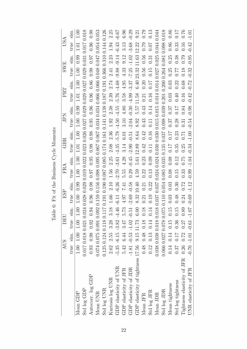
Table6:

Fitof

theBusinessCycle

Mom

ents

AUS

DEU

ESP

FRA

GBR

JPN

PRT

SWE

USA

true

sim.

true

sim.

true

sim.

true

sim.

true

sim.

true

sim.

true

sim.

true

sim.

true

sim.

MeanGDP

1.00

1.00

1.00

1.00

1.00

0.99

1.00

1.00

1.01

1.00

1.00

0.99

1.01

1.00

1.00

0.99

1.01

1.00

StdlogGDP

0.0170.0180.0210.0240.0280.0290.0190.0220.0230.0260.0270.0290.0290.0270.0290.0310.0170.018

Autocorr.

logGDP

0.93

0.98

0.92

0.94

0.96

0.98

0.97

0.95

0.98

0.98

0.95

0.96

0.96

0.86

0.98

0.97

0.96

0.98

MeanUNR

0.0740.0750.0910.0920.1590.1560.0980.0950.0670.0670.0340.0340.0660.0660.0480.0470.0540.053

StdlogUNR

0.1250.1240.1180.1170.1910.1900.0870.0850.1740.1610.1410.1380.1870.1910.3660.3100.1440.126

KurtosislogUNR

2.62

2.55

3.28

3.18

1.66

2.10

1.56

2.25

2.08

2.36

1.92

2.38

2.39

2.74

2.41

2.23

1.94

2.25

GDP

elasticity

ofUNR

-5.35

-6.15

-3.82

-4.46

-6.11

-6.26

-2.70

-3.61

-4.35

-5.78

-4.50

-4.55

-5.76

-4.68

-9.88

-9.14

-6.43

-6.67

GDP

elasticity

ofJF

R5.42

6.44

3.47

5.73

4.97

7.41

5.55

4.28

3.14

6.01

3.10

4.80

3.58

4.95

4.33

9.12

3.13

6.96

GDP

elasticity

ofJD

R-1.81

-0.53

-1.02

-0.51

-2.69

-0.58

0.29

-0.45

-2.90

-0.51

-2.04

-0.30

-4.99

-3.37

-7.25

-1.02

-3.68

-0.29

GDP

elasticity

oftigh

tness17.56

9.15

11.73

6.00

8.32

10.40

4.59

5.61

12.89

8.64

8.92

5.57

11.58

6.40

23.3211.6312.22

9.21

MeanJF

R0.48

0.48

0.18

0.18

0.21

0.21

0.22

0.23

0.42

0.42

0.43

0.43

0.21

0.20

0.56

0.56

0.79

0.79

StdlogJF

R0.12

0.13

0.14

0.14

0.19

0.22

0.13

0.09

0.11

0.16

0.11

0.14

0.16

0.17

0.15

0.31

0.07

0.13

MeanJD

R0.0380.0380.0180.0180.0370.0370.0240.0240.0300.0300.0150.0150.0140.0140.0270.0250.0440.044

StdlogJD

R0.0660.0270.0780.0750.1100.0540.0850.0350.1350.0370.0980.0390.2010.2000.2640.0810.0980.018

Meantigh

tness

0.14

0.14

0.15

0.15

0.03

0.03

0.08

0.08

0.17

0.17

0.37

0.37

0.03

0.03

0.25

0.25

0.86

0.86

Stdlogtigh

tness

0.37

0.17

0.36

0.15

0.48

0.30

0.15

0.12

0.35

0.23

0.28

0.17

0.40

0.22

0.77

0.38

0.33

0.17

Tightness

elasticity

ofJF

R0.26

0.72

0.27

0.89

0.24

0.72

0.33

0.75

0.25

0.71

0.31

0.84

0.16

0.68

0.18

0.79

0.16

0.76

UNR

elasticity

ofJF

R-0.76

-1.01

-0.61

-1.07

-0.69

-1.12

-0.99

-1.04

-0.34

-1.00

-0.54

-0.98

-0.42

-0.72

-0.32

-0.95

-0.42

-1.01

22

Table 7: Correlation Between Actual and Predicted Detrended Series

AUS FRA DEU JAP PRT ESP SWE GBR USA AverageProductivity 1.00 1.00 1.00 1.00 1.00 1.00 1.00 1.00 1.00 1.00Unemployment 0.83 0.68 0.88 0.87 0.73 0.92 0.77 0.87 0.75 0.81Job Finding Rate 0.70 0.64 0.70 0.79 0.74 0.77 0.31 0.85 0.82 0.70Job Destruction Rate 0.16 0.03 0.32 0.02 -0.06 0.20 0.36 0.23 0.34 0.18Market Tightness 0.71 0.63 0.38 0.51 0.83 0.84 0.43 0.67 0.65 0.63

1985 1995 2005

6

8

10

Cyclic

al

unem

plo

ym

ent

AUS

1985 1995 20056

8

10

12DEU

1985 1995 200510

15

20

ESP

1985 1995 20058

9

10

11

Cyclic

al

un

em

plo

ym

ent

FRA

1985 1995 20054

6

8

10GBR

1985 1995 20052

3

4

JPN

1985 1995 20054

6

8

10

Cyclic

al

unem

plo

ym

ent

PRT

1985 1995 2005

2

4

6

8

10SWE

1985 1995 2005

4

6

8USA

Figure 2: Unemployment Cycle - Actual (solid line) and Simulated (dotted)

23

A thick left tail of the distribution of worker heterogeneity amplifies the recessive effect

of negative productivity shocks. If the recession lasts, unemployment increases because

low-ability workers remain unemployed longer. When the economy recovers, previously

unproductive workers become productive again, and they progressively start to get back

to work. The process of layoff and reemployment is dissymmetric: all unproductive

workers are immediately laid off, while all unemployed, but productive, workers are not

instantaneously reemployed.

The fit of job finding rates is also good, with accurate estimates of volatility. However,

the elasticity of job finding rates with respect to tightness (respectively to unemployment)

is greatly over-estimated (resp. under-estimated). Although the correlation between

actual and predicted series of tightness is good (around 65%), we generally greatly under-

estimate its volatility. These two findings (the excess sensitivity of the job finding rate to

market tightness and the under-estimation of the volatility of tightness) are related. The

response of vacancy creation to productivity shocks has to be attenuated, or job finding

rates would not be well fitted. Additional friction (such as the negative dependence of

job finding rates to unemployment duration) is therefore required to make the job finding

process more sluggish in recovery times.

Finally, the job destruction rate that is predicted by the model is too unevenly dented,

and its correlation to actual series is poor. This may happen again because the process

of endogenous job destruction is too lumpy. Following a negative productivity shocks,

a mass of workers is instantly laid off, and the job destruction rate is immediately after

reverted to the frictional rate of exogenous job destruction unless aggregate productivity

keeps going further down.

We will see in the next section that this apparent failure at fitting some aspects of

turnover and vacancies could be an artifact of detrending (using the Hodrick-Prescott

filter). If total output is clearly trended and easily detrended, long-term trends in labor

market variables are much more difficult to filter out. This is the reason why Shimer

(2005), and his followers, including us, used the HP filter with a smoothing parameter

of 105, much greater than the standard value of 1024 recommended for quarterly series.

24

Using 1024 yields a trend of unemployment that undulates like a cycle. In the next section,

we will argue that a better way of handling trends in labor market variables is to model

them by way of intervention variables (policy or demographics).

6 The impact of labor market reforms

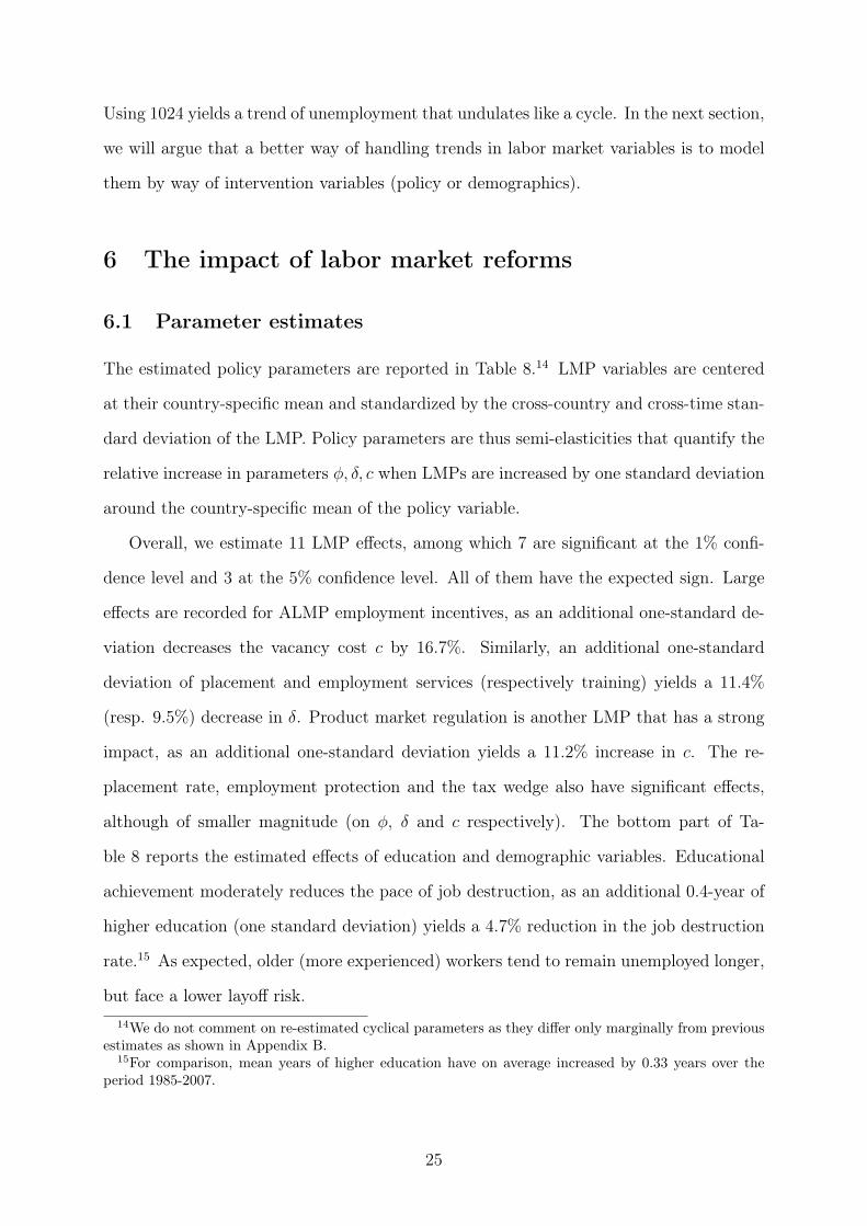
6.1 Parameter estimates

The estimated policy parameters are reported in Table 8.14 LMP variables are centered

at their country-specific mean and standardized by the cross-country and cross-time stan-

dard deviation of the LMP. Policy parameters are thus semi-elasticities that quantify the

relative increase in parameters φ, δ, c when LMPs are increased by one standard deviation

around the country-specific mean of the policy variable.

Overall, we estimate 11 LMP effects, among which 7 are significant at the 1% confi-

dence level and 3 at the 5% confidence level. All of them have the expected sign. Large

effects are recorded for ALMP employment incentives, as an additional one-standard de-

viation decreases the vacancy cost c by 16.7%. Similarly, an additional one-standard

deviation of placement and employment services (respectively training) yields a 11.4%

(resp. 9.5%) decrease in δ. Product market regulation is another LMP that has a strong

impact, as an additional one-standard deviation yields a 11.2% increase in c. The re-

placement rate, employment protection and the tax wedge also have significant effects,

although of smaller magnitude (on φ, δ and c respectively). The bottom part of Ta-

ble 8 reports the estimated effects of education and demographic variables. Educational

achievement moderately reduces the pace of job destruction, as an additional 0.4-year of

higher education (one standard deviation) yields a 4.7% reduction in the job destruction

rate.15 As expected, older (more experienced) workers tend to remain unemployed longer,

but face a lower layoff risk.14We do not comment on re-estimated cyclical parameters as they differ only marginally from previous

estimates as shown in Appendix B.15For comparison, mean years of higher education have on average increased by 0.33 years over the

period 1985-2007.

25

Table 8: Estimates of Policy Effects

φ δ c

Initial replacement rate -0.030 0.031(0.008) (0.009)

ALMP Placement and 0.028 -0.102Employment Services (0.006) (0.007)ALMP Training -0.044 -0.100

(0.016) (0.019)ALMP Incentives 0.061 -0.165

(0.020) (0.057)Product Market Regulation -0.025 0.115

(0.018) (0.051)Employment Protection -0.023 -0.038(regular contracts) (0.007) (0.008)Tax wedge 0.023 0.045

(0.008) (0.022)Mean Years of -0.010 -0.050Higher Education (0.008) (0.009)Share 15-24 population 0.016 -0.019

(0.010) (0.012)Share 55-64 population -0.027 -0.053

(0.006) (0.007)

6.2 Fitting the trends

Figures 3-6 show how good the model is at predicting labor market outcomes given pro-

ductivity shocks and institutional change. Table 9 displays the correlations between actual

and predicted series. Actual and simulated unemployment rates are highly correlated for

all countries, with an average correlation equal to 0.81. The best fit is obtained for Aus-

tralia, Japan, Sweden and the United Kingdom with correlations close to or above 0.90,

while the model performs less well for the United States with a correlation of about 0.5.

The fit of job destruction rates is greatly improved by comparison to the cyclical

estimation, as the correlation between predicted and observed series jumps from 0.18 in

the BC-model to 0.57 in the LMP-model. The fit of job finding rates, which are well

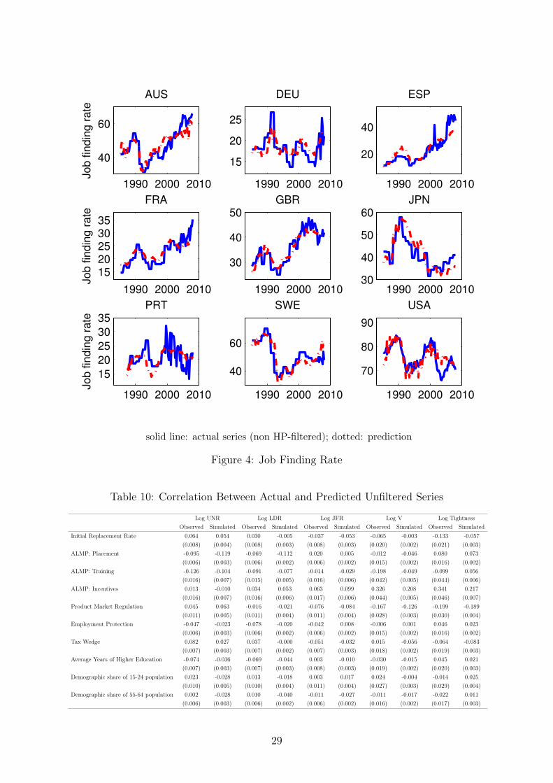
predicted except for Germany and Portugal, and the US to a lesser extent, has also

improved. Market tightness is well fitted for all countries but the US and Portugal.

The only country for which the model does not seem to be doing such a good job

is the US. It may be that by estimating LMP effects jointly we impose to the US labor

26

market a European norm that does not apply to the US. It may also be that simulating

the economy at the quarterly frequency does not work well for the US, as very few workers

remain unemployed longer than a quarter. Yet, overall, these results suggest that LMPs

help predict the permanent shifts in unemployment and its turnover components well.

We then ask whether the simulated series in Figures 3-6 reproduce the correlations

with LMP variables that were estimated in the reduced-form regressions of Table 4. Table

10 shows comparisons. In general the fit is quite good. The model

6.3 Assessing the Impact of Labor Market Policies

In order to get a sense of the marginal effect of each policy on unemployment, we proceeded

to the following comparison. For each country, we calculate a benchmark unemployment

value by setting LMPs at their country-specific mean values and simulating very long

series of productivity shocks and implied labor market outcomes. We then calculate

the resulting mean unemployment rate over time. In a second step, we calculate the

counterfactual steady-state unemployment rates that result from a one-standard deviation

(cross-time and cross-country) change in the LMPs. The choice of the direction is chosen

in accordance to our prior on the effect of the policy on unemployment.

Table 11 reports the results. The top-panel displays the benchmark values of unem-

ployment rates, job finding and job destruction rates, and vacancies. The bottom-panel

shows counterfactual changes. In so far as the size of the assumed changes do represent

commensurate and comparable policy reforms, the LMP the most conducive to unem-

ployment reduction appears to be placement and employment services (-0.94 percentage

points on average). All other LMPs have a similar influence, between a fifth and a third

of a percentage point.

At the bottom of Table 11, we report the sum of individual LMP-effects, as well as

the calculated effect on unemployment of a simultaneous change in all LMPs (labelled

as the “policy mix"). We do not find evidence of policy complementarity, as the sum

of individual effects is only (and always) slightly larger than the impact of the policy

mix. This finding contradicts Bassanini and Duval (2009), who found positive interaction

27

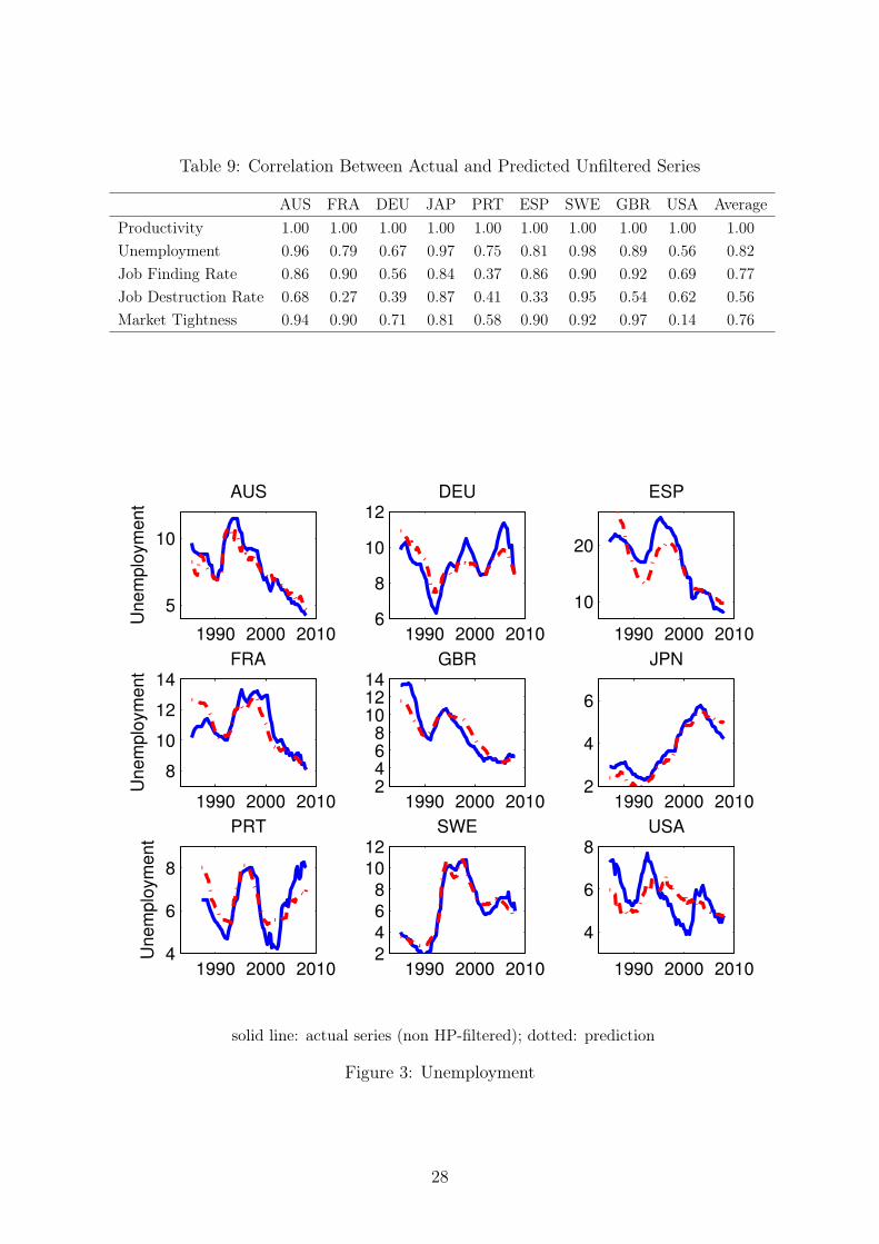
Table 9: Correlation Between Actual and Predicted Unfiltered Series

AUS FRA DEU JAP PRT ESP SWE GBR USA AverageProductivity 1.00 1.00 1.00 1.00 1.00 1.00 1.00 1.00 1.00 1.00Unemployment 0.96 0.79 0.67 0.97 0.75 0.81 0.98 0.89 0.56 0.82Job Finding Rate 0.86 0.90 0.56 0.84 0.37 0.86 0.90 0.92 0.69 0.77Job Destruction Rate 0.68 0.27 0.39 0.87 0.41 0.33 0.95 0.54 0.62 0.56Market Tightness 0.94 0.90 0.71 0.81 0.58 0.90 0.92 0.97 0.14 0.76

1990 2000 2010

5

10

Unem

plo

ym

ent

AUS

1990 2000 20106

8

10

12DEU

1990 2000 2010

10

20

ESP

1990 2000 2010

8

10

12

14

Unem

plo

ym

ent

FRA

1990 2000 20102468

101214

GBR

1990 2000 20102

4

6

JPN

1990 2000 20104

6

8

Une

mplo

ym

ent

PRT

1990 2000 20102

4

6

8

10

12SWE

1990 2000 2010

4

6

8USA

solid line: actual series (non HP-filtered); dotted: prediction

Figure 3: Unemployment

28

1990 2000 2010

40

60

Job fin

din

g r

ate

AUS

1990 2000 2010

15

20

25

DEU

1990 2000 2010

20

40

ESP

1990 2000 2010

1520253035

Job fin

din

g r

ate

FRA

1990 2000 2010

30

40

50GBR

1990 2000 201030

40

50

60JPN

1990 2000 2010

15

20

25

30

35

Jo

b fin

din

g r

ate

PRT

1990 2000 2010

40

60

SWE

1990 2000 2010

70

80

90

USA

solid line: actual series (non HP-filtered); dotted: prediction

Figure 4: Job Finding Rate

Table 10: Correlation Between Actual and Predicted Unfiltered Series

Log UNR Log LDR Log JFR Log V Log TightnessObserved Simulated Observed Simulated Observed Simulated Observed Simulated Observed Simulated

Initial Replacement Rate 0.064 0.054 0.030 -0.005 -0.037 -0.053 -0.065 -0.003 -0.133 -0.057(0.008) (0.004) (0.008) (0.003) (0.008) (0.003) (0.020) (0.002) (0.021) (0.003)

ALMP: Placement -0.095 -0.119 -0.069 -0.112 0.020 0.005 -0.012 -0.046 0.080 0.073(0.006) (0.003) (0.006) (0.002) (0.006) (0.002) (0.015) (0.002) (0.016) (0.002)

ALMP: Training -0.126 -0.104 -0.091 -0.077 -0.014 -0.029 -0.198 -0.049 -0.099 0.056(0.016) (0.007) (0.015) (0.005) (0.016) (0.006) (0.042) (0.005) (0.044) (0.006)

ALMP: Incentives 0.013 -0.010 0.034 0.053 0.063 0.099 0.326 0.208 0.341 0.217(0.016) (0.007) (0.016) (0.006) (0.017) (0.006) (0.044) (0.005) (0.046) (0.007)

Product Market Regulation 0.045 0.063 -0.016 -0.021 -0.076 -0.084 -0.167 -0.126 -0.199 -0.189(0.011) (0.005) (0.011) (0.004) (0.011) (0.004) (0.028) (0.003) (0.030) (0.004)

Employment Protection -0.047 -0.023 -0.078 -0.020 -0.042 0.008 -0.006 0.001 0.046 0.023(0.006) (0.003) (0.006) (0.002) (0.006) (0.002) (0.015) (0.002) (0.016) (0.002)

Tax Wedge 0.082 0.027 0.037 -0.000 -0.051 -0.032 0.015 -0.056 -0.064 -0.083(0.007) (0.003) (0.007) (0.002) (0.007) (0.003) (0.018) (0.002) (0.019) (0.003)

Average Years of Higher Education -0.074 -0.036 -0.069 -0.044 0.003 -0.010 -0.030 -0.015 0.045 0.021(0.007) (0.003) (0.007) (0.003) (0.008) (0.003) (0.019) (0.002) (0.020) (0.003)

Demographic share of 15-24 population 0.023 -0.028 0.013 -0.018 0.003 0.017 0.024 -0.004 -0.014 0.025(0.010) (0.005) (0.010) (0.004) (0.011) (0.004) (0.027) (0.003) (0.029) (0.004)

Demographic share of 55-64 population 0.002 -0.028 0.010 -0.040 -0.011 -0.027 -0.011 -0.017 -0.022 0.011(0.006) (0.003) (0.006) (0.002) (0.006) (0.002) (0.016) (0.002) (0.017) (0.003)

29

1990 2000 2010

3

3.5

4

4.5

Job d

estr

uction r

ate AUS

1990 2000 20101.4

1.6

1.8

2

2.2

DEU

1990 2000 2010

3

4

5

ESP

1990 2000 2010

2

3

4

Job d

estr

uction r

ate FRA

1990 2000 2010

2

4

GBR

1990 2000 2010

1

1.5

2

JPN

1990 2000 2010

1

1.5

2

Job d

estr

uction r

ate PRT

1990 2000 2010

2

4

SWE

1990 2000 2010

4

6

USA

solid line: actual series (non HP-filtered); dotted: prediction

Figure 5: Job Destruction Rate

30

1990 2000 20100

0.2

0.4

Mark

et tightn

ess

AUS

1990 2000 2010

0.05

0.1

0.15

DEU

1990 2000 20100

0.05

0.1

ESP

1990 2000 2010

0.05

0.1

0.15

Mark

et tightn

ess

FRA

1990 2000 20100

0.5

GBR

1990 2000 2010

0.2

0.4

JPN

1990 2000 2010

0.02

0.04

0.06

0.08

Mark

et tightn

ess

PRT

1990 2000 20100

0.5

SWE

1990 2000 2010

0.4

0.6

0.8

1

1.2

USA

solid line: actual series (non HP-filtered); dotted: prediction

Figure 6: Market Tightness

31

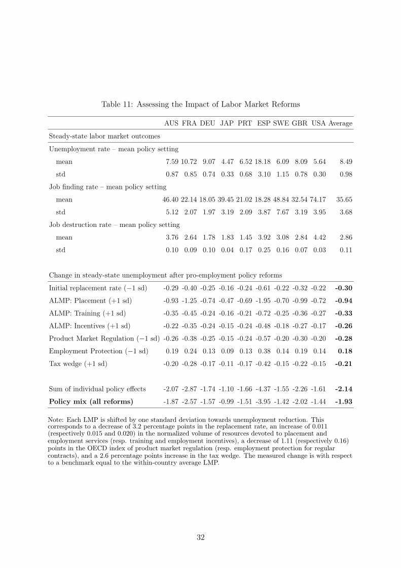
Table 11: Assessing the Impact of Labor Market Reforms

AUS FRA DEU JAP PRT ESP SWE GBR USA Average

Steady-state labor market outcomes

Unemployment rate – mean policy setting

mean 7.59 10.72 9.07 4.47 6.52 18.18 6.09 8.09 5.64 8.49

std 0.87 0.85 0.74 0.33 0.68 3.10 1.15 0.78 0.30 0.98

Job finding rate – mean policy setting

mean 46.40 22.14 18.05 39.45 21.02 18.28 48.84 32.54 74.17 35.65

std 5.12 2.07 1.97 3.19 2.09 3.87 7.67 3.19 3.95 3.68

Job destruction rate – mean policy setting

mean 3.76 2.64 1.78 1.83 1.45 3.92 3.08 2.84 4.42 2.86

std 0.10 0.09 0.10 0.04 0.17 0.25 0.16 0.07 0.03 0.11

Change in steady-state unemployment after pro-employment policy reforms

Initial replacement rate (−1 sd) -0.29 -0.40 -0.25 -0.16 -0.24 -0.61 -0.22 -0.32 -0.22 -0.30

ALMP: Placement (+1 sd) -0.93 -1.25 -0.74 -0.47 -0.69 -1.95 -0.70 -0.99 -0.72 -0.94

ALMP: Training (+1 sd) -0.35 -0.45 -0.24 -0.16 -0.21 -0.72 -0.25 -0.36 -0.27 -0.33

ALMP: Incentives (+1 sd) -0.22 -0.35 -0.24 -0.15 -0.24 -0.48 -0.18 -0.27 -0.17 -0.26

Product Market Regulation (−1 sd) -0.26 -0.38 -0.25 -0.15 -0.24 -0.57 -0.20 -0.30 -0.20 -0.28

Employment Protection (−1 sd) 0.19 0.24 0.13 0.09 0.13 0.38 0.14 0.19 0.14 0.18

Tax wedge (+1 sd) -0.20 -0.28 -0.17 -0.11 -0.17 -0.42 -0.15 -0.22 -0.15 -0.21

Sum of individual policy effects -2.07 -2.87 -1.74 -1.10 -1.66 -4.37 -1.55 -2.26 -1.61 -2.14

Policy mix (all reforms) -1.87 -2.57 -1.57 -0.99 -1.51 -3.95 -1.42 -2.02 -1.44 -1.93

Note: Each LMP is shifted by one standard deviation towards unemployment reduction. Thiscorresponds to a decrease of 3.2 percentage points in the replacement rate, an increase of 0.011(respectively 0.015 and 0.020) in the normalized volume of resources devoted to placement andemployment services (resp. training and employment incentives), a decrease of 1.11 (respectively 0.16)points in the OECD index of product market regulation (resp. employment protection for regularcontracts), and a 2.6 percentage points increase in the tax wedge. The measured change is with respectto a benchmark equal to the within-country average LMP.

32

effects on the basis of panel-data, reduced-form regressions.

Finally, identical labor market reforms seem to trigger very different unemployment

responses (in magnitude) across countries, with high-unemployment countries such as

Spain or France witnessing larger unemployment reductions than the other countries.

33

7 Conclusion

We have proposed a non-stationary dynamic search-matching model with worker hetero-

geneous abilities and labor market policy interventions. Worker heterogeneity makes the

effect of negative productivity shocks on unemployment highly non linear, and provides an

amplification mechanism solving the unemployment volatility puzzle. Policy interventions

shift structural parameters such as matching efficiency, exogenous job destruction and va-

cancy cost, and have long term effects on unemployment. For all 9 OECD countries, the

model displays an impressive fit of unemployment dynamics. The amount of resources

injected into placement and employment services stands out as the most prominent pol-

icy lever in view of reducing unemployment. All other LMPs have a significant but lesser

impact. We also find that the magnitude of the effect is larger for high-unemployment

countries, and we find little complementarity between policies.

In its present form, the model remains too simple to adequately capture all aspects

of labor market institutions. For example, an important operating mechanism is search

intensity, which is not explicitly modeled here (only through an exogenous change in

matching efficiency). Moreover, unemployment benefits are always paid for a fixed period

of time, thus introducing state dependence in search intensity. These are just a few out

of many possible ideas for future extensions.

34

References

[1] Bassanini, A., and R. Duval (2009), “Unemployment, Institutions and Re-

form Complementarities: Re-Assessing the Aggregate Evidence for OECD

Countries", Oxford Review of Economic Policy,Vol. 25(1), pp. 40-59.

[2] Bertola, G., Blau, F. and L. Kahn (2007), “Labor market institutions and

demographic employment patterns," Journal of Population Economics, vol.

20(4), pp. 833-867.

[3] Blanchard, O. and J. Wolfers (2000), “The Role of Shocks and Institutions in

the Rise of European Unemployment: The Aggregate Evidence", Economic

Journal, vol.110 (462), pp. C1-33.

[4] Bruno, M., and J. Sachs (1985), “Economics of Worldwide Stagflation", Har-

vard University Press, Cambridge, MA, pp. vii+315.

[5] Chadic, P. and F. Postel-Vinay (2002), “Temporary Jobs, Employment Pro-

tection and Labor Market Performance", Labor Economics No. 9, pp. 63-

91.

[6] Elsby, M., B. Hobijn and A. Sahin (2012), “Unemployment Dynamics in the

OECD", forthcoming Review of Economics and Statistics.

[7] Felbermayr, G. and J. Prat (2011), “Product Market Regulation, Firm Selec-

tion and Unemployment”, Journal of the European Economic Association,

Vol. 9 (2), pp. 278-318.

[8] Gertler, M., and A. Trigari (2009), “Unemployment Fluctuations with Stag-

gered Nash Wage Bargaining", Journal of Political Economy, University of

Chicago Press, Vol. 117(1), pp. 38-86, 02.

[9] Hagedorn, M., and I. Manovskii (2008), “The Cyclical Behavior of Equilib-

rium Unemployment and Vacancies Revisited", American Economic Review,

Vol. 98(4), pp. 1692-1706.

35

[10] Hall, R.E. (2005), “Employment Fluctuations with Equilibrium Wage Stick-

iness". American Economic Review, Vol. 95(1), pp. 50-65.

[11] Hall, R.E., and A.B. Krueger (2012), “Evidence on the Incidence of Wage

Posting, Wage Bargaining, and on-the-Job Search”, American Economic

Journal: Macroeconomics, vol.4(4), pp. 56-67.

[12] Hall, R.E. and P.R. Milgrom (2008), “The Limited Influence of Unemploy-

ment on the Wage Bargain," American Economic Review, vol. 98(4), pp.

1653-74.

[13] Jolivet, G., Postel-Vinay, F. and J.M. Robin (2006), “The Empirical Content

of the Job Search Model: Labor Mobility and Wage Distribution in Europe

and the U.S.", European Economic Review, vol.50, 877-907.

[14] Lise and Robin (2013), “The Macro-dynamics of Sorting between Workers

and Firms”, mimeo.

[15] Ljungqvist, L. and T.J. Sargent (1998), The European Unemployment

Dilemma," Journal of Political Economy, vol. 106(3), pp. 514-550.

[16] Mortensen, D., and C. Pissarides (1994),“Job Creation and Job Destruc-

tion in the Theory of Unemployment", The Review of Economic Studies,

Vol.61(3), pp. 397-415.

[17] Murrain, F., and A. de Serres, (2013), “How Do Policies Affect the Exit

Rate Out of Unemployment: Disentangling Job Creation from Labor Market

Frictions", forthcoming OECD working paper.

[18] Murrain, F., de Serres, A. and A. Hijzen, (2013), “Unemployment Turnover

and the Automatic Extension of Collective Wage Agreements", forthcoming

OECD working paper.

[19] Pissarides, C. (2009), “The Unemployment Volatility Puzzle: Is Wage Stick-

iness the Answer?", Econometrica, Vol. 77(5), pp. 1339-1369, 09.

36

[20] Postel-Vinay, F., and J.M. Robin (2002), “Equilibrium Wage Dispersion with

Worker and Employer Heterogeneity", Econometrica, 70(6), pp. 2295-350.

[21] Felbermayr, G., and J. Pratt (2011), “Product Market Regulation, Firm Se-

lection, and Unemployment”, Journal of the European Economic Association,

pp. 278-317.

[22] Prescott, E. C. (2004), “Why Do Americans Work So Much More Than Euro-

peans?", Federal Reserve Bank of Minneapolis Quarterly Review, vol.28(1),

pp.2-13.

[23] Nickell, S. and R. Layard (1999), “Labor market institutions and economic

performance," Handbook of Labor Economics, in: O. Ashenfelter and D.

Card (ed.), Handbook of Labor Economics, edition 1, volume 3, chapter 46,

pp. 3029-3084, Elsevier.

[24] Robin, J.M. (2011), “On the Dynamics of Unemployment and Wage Distri-

butions", Econometrica, Vol.79(5), pp.1327.

[25] Rogerson, R. (2008), “Structural Transformation and the Deterioration

of European Labor Market Outcomes," Journal of Political Economy,

vol.116(2), pp. 235-259, 04.

[26] Shimer, R. (2005), “The Cyclical Behavior of Equilibrium Unemployment

and Vacancies", The American Economic Review, vol.95(1), pp. 25-49.

37