Lab 3: Low-Speed Delta Wing - psp-tsp.compsp-tsp.com/pdfs/Labs/Lab 3_Low Speed Delta.pdf · Lab 3:...

2009

Innovative Scientific Solutions Inc.

2766 Indian Ripple Road

Dayton, OH 45440

(937)-429-4980

Lab 3: Low-Speed Delta Wing

Lab 3: Low-Speed Delta Wing Page 1

Lab 3: Low-Speed Delta Wing

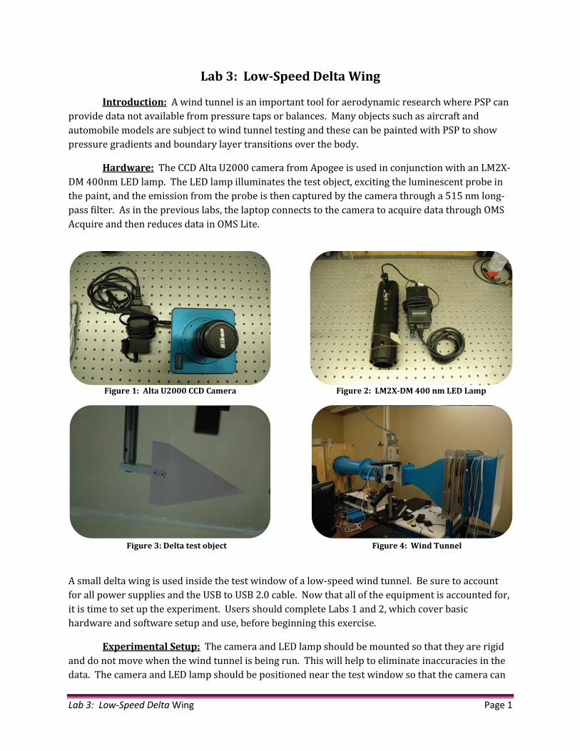
Introduction: A wind tunnel is an important tool for aerodynamic research where PSP can

provide data not available from pressure taps or balances. Many objects such as aircraft and

automobile models are subject to wind tunnel testing and these can be painted with PSP to show

pressure gradients and boundary layer transitions over the body.

Hardware: The CCD Alta U2000 camera from Apogee is used in conjunction with an LM2X-

DM 400nm LED lamp. The LED lamp illuminates the test object, exciting the luminescent probe in

the paint, and the emission from the probe is then captured by the camera through a 515 nm long-

pass filter. As in the previous labs, the laptop connects to the camera to acquire data through OMS

Acquire and then reduces data in OMS Lite.

A small delta wing is used inside the test window of a low-speed wind tunnel. Be sure to account

for all power supplies and the USB to USB 2.0 cable. Now that all of the equipment is accounted for,

it is time to set up the experiment. Users should complete Labs 1 and 2, which cover basic

hardware and software setup and use, before beginning this exercise.

Experimental Setup: The camera and LED lamp should be mounted so that they are rigid

and do not move when the wind tunnel is being run. This will help to eliminate inaccuracies in the

data. The camera and LED lamp should be positioned near the test window so that the camera can

Figure 1: Alta U2000 CCD Camera Figure 2: LM2X-DM 400 nm LED Lamp

Figure 3: Delta test object Figure 4: Wind Tunnel


focus on the test object and the LED lamp can uniformly illuminate the surface as shown in Figure 5.

To avoid noise in your images, place the lamp and camera at different angles so the light reflected

back into the camera is minimal. Attach all power supplies to the camera, LED lamp, and the

computer. Attach the USB to USB 2.0 cable and the computer should recognize the connection

automatically. More details of experimental setup and data acquisition are explained in Lab 2.

The wind tunnel has a test section window where the test object is to be placed. Mount the test

object so that it is in the center of the test section. The angle at which the delta plane encounters

the flow can be adjusted to the user’s liking by turning the knob on the top plate of the window

which holds the delta.

Figure 5: Experimental Setup

Figure 6: Wind tunnel test section


In wind tunnel tests where the test body is likely to move or deflect during data acquisition,

it is necessary to use markers for image alignment. Markers can be physically placed on the test

object by simply marking the painted surface with a sharpie or pen. This will show up on the wind-

off and wind-on images as an area with little illumination since the paint is not visible. The user can

use these reference points to create their markers. Figure 7 shows an example of markers placed

on the test object prior to data acquisition. As discussed in the image alignment section below, the

number of markers is important for the movement correction process. For this exercise 8 markers

is sufficient.

Figure 7: Example of markers

Data Acquisition: In OMS Acquire ( ), use the live preview ( ) to view the image

seen by the camera and adjust the camera’s focus so that the image in the preview is clear. Be sure

to turn off or block any light sources to avoid noise in your data before data acquisition begins.

Place the delta at a slight angle of attack (5-10 degrees) and mount securely in the test section.

Capture the background image with the room lighting and the LED lamp turned off. Save the

background image (bkground.tif) in a new folder where all images will be stored. Create a new file

each time a new image with different settings is captured by pressing the icon in the upper left

area of OMS Acquire next to the file path description. We will demonstrate the frame average

function and its improvement to the signal-to-noise ratio. Capture the wind-off images with the

wind tunnel off. Set the frames to average ( ) to 4 and the exposure to a level where

the image is not saturated. Turn the LED lamp on and allow it to stabilize before taking data.

Capture wind-off images for frame averages of 4, 16, and 64 and save them each accordingly


(Example: wind_off_XXXms_Xfr.tif). It is good practice to include some detail in the file name so it is

easier to decipher later on when processing the data.

Turn on your wind tunnel and set it to the desired airspeed and allow it to stabilize. All data

shown here was run at 30 m/s (~Mach 0.1). Once the tunnel is up to speed the data acquisition can

begin. Save the image with a name that will reference your test condition settings for exposure

time, airspeed, and frames averaged (Example: wind_on_XXXms_Xmps_Xfr.tif). If when processing

the images in OMS Lite the images do not appear to have an acceptable resolution, it may be

necessary to average more frames to capture the pressure distribution. This is only one factor since

exposure time, shot noise, and wind tunnel speed also have an effect on your data. Lower speeds

present a more difficult case since the pressure variation across the surface is very low. It will be

important to improve the signal-to-noise ratio as best as possible so that the pressure map can be

seen. Frame averaging will greatly improve your data at low speeds as will taking time to block out

any ambient light in the room. Doing this will greatly improve the signal-to-noise ratio and

therefore, the final data.

Data Reduction: Reducing the data into an image of pressure involves taking the ratio of

the wind-off / wind-on images and then calibrating the image to relate the ratio to pressure. Create

a new project in OMS Lite ( ) using the PSP

Single Channel option. Select the folder that the

data files taken are saved in. Save the project as

low_speed_delta.ims. In the GUI for the Single

Channel tab in OMS Lite, load the wind-off,

wind-on, and background images for the case of

4 frames averaged at 30 m/s. While selecting

from the list of images at these conditions, you

will notice that there are four images saved for

each data point taken (Figure 10). One of these images is the signal channel (pressure) and the

others are reference channels. In the case of the camera used in this test, the signal channel was 1,

but that may differ from camera to camera. The signal channel is the channel that should be used in

data reduction. To determine what channel is the signal channel, load each image into OMS Lite and

examine them by using the icon. The image with the highest intensity will be the signal

channel. Notice in Figures 11 and 12 below, the difference in intensity on the right hand toolbar

and in the color of the images.

Figure 10: Locating the signal channel


Figure 11: Signal Channel Uncorrected Image (Wind-Off)

Figure 12: Reference Channel Uncorrected Image (Wind-Off)

The yellow and orange image is the signal and the blue image is the reference channel. The

signal channel goes up to around 39000 counts in intensity while the reference only goes up to

about 11000 counts. Once this is known for one case it will remain the same for all. The signal

channel will not change from case to case; it is constant for each camera. The same background

image may be used in all cases and should be the signal channel as well. Examine the wind-off and

wind-on images and set the dark threshold near to the signal level of the background of the image

(colored pink in Figures 11 and 12).

Process the data without filtering or aligning: If we first process the data without using

any of the filtering or alignment options, we can see the improvement those features provide. The


image used here was the 4 frame averaged. Do not apply any of the filters or markers when

creating the ratio image. Load the paint calibration file BF405.clb and enter the test conditions for

your experiment (Mach = 0.1, atmospheric temperature and pressure, dynamic pressure of ~500 Pa

and α = 15, β = 0). Compute the pressure image and adjust the paint minimum and maximum levels

so that you see an image with clarity similar to Figure 13. Use this image as a reference for the

filtered and aligned images to check for improvement.

Figure 13: Unfiltered Pressure Image (4 Frame average, 30 m/s)

Low-Pass Filters: The smoothing filter is a low-pass filter that filters by the specified pixel

diameter. Use the Gauss filter and chose a large pixel diameter to filter out spottiness on the image.

Adjust the color palette and the paint minimum and maximum to see the most detail in your image.

Use the legend to determine the best intensity range for your image. This process will also improve

the signal-to-noise ratio. If you are averaging 16 images and running a 16 pixel low-pass filter

(Figure 15), it should yield a factor of improvement of 64 in signal-to-noise over a single shot image

(sqrt(16*16*16)=64). Compare Figure 15 to the 4 pixel filtered, 4 frame averaged image shown in

Figure 14. Notice the splotchy colors in Figure 14. The low-pass filter and increased frames

averaged smooth the image giving a more defined representation of the pressure field with a much

better signal-to-noise ratio.


Figure 15: Ratio Image with Low-Pass Filter (16 pixels, 16 frames)

Use the tool to compare graphically, the noise reduction from the unfiltered image to the two

filtered images. Left click drag and release the cursor to create a graph of the pressure distribution.

Repeat the same process for the higher frame averaged images to see the effects of the low-pass

filter.

Figure 14: Ratio Image with Low-Pass filter (4 pixels, 4 frames)


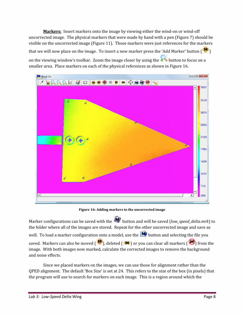
Markers: Insert markers onto the image by viewing either the wind-on or wind-off

uncorrected image. The physical markers that were made by hand with a pen (Figure 7) should be

visible on the uncorrected image (Figure 11). Those markers were just references for the markers

that we will now place on the image. To insert a new marker press the ‘Add Marker’ button ( )

on the viewing window’s toolbar. Zoom the image closer by using the button to focus on a

smaller area. Place markers on each of the physical references as shown in Figure 16.

Figure 16: Adding markers to the uncorrected image

Marker configurations can be saved with the button and will be saved (low_speed_delta.mrk) to

the folder where all of the images are stored. Repeat for the other uncorrected image and save as

well. To load a marker configuration onto a model, use the button and selecting the file you

saved. Markers can also be moved ( ), deleted ( ) or you can clear all markers ( ) from the

image. With both images now marked, calculate the corrected images to remove the background

and noise effects.

Since we placed markers on the images, we can use those for alignment rather than the

QPED alignment. The default ‘Box Size’ is set at 24. This refers to the size of the box (in pixels) that

the program will use to search for markers on each image. This is a region around which the


markers could have moved, i.e. you are telling

the program that no marker moved more than

24 pixels from its wind-off location as a result of

object movement.

‘Fix first’ refers to which marker point

will be fixed.

Order refers to the order of the curve fit.

0 is appropriate for a simple solid body

movement. Higher order fits are used to deal

with bending and rotating displacements

however, they do give you odd behavior outside

of the marker boundary. A minimum number of

markers are required for each curve fit since the

polynomial order dictates the number of

unknowns. Since we have eight markers in this

experiment, we cannot exceed a second-order

polynomial. For a low-speed experiment like

this one, there is very little movement of the test

body and therefore it is difficult to notice any

changes in the image due to alignment alone. Both the QPED and marker alignments can be used

together if desired.

There are three types of low-pass or smoothing filters; Gauss, Flat, and Median. The low-

pass filter is a spatial averaging of the size the user enters for Dx and Dy. The Gauss filter applies a

Gaussian distribution filter to the image, the Flat filter applies a flat filtering to the image, and the

Median filter applies a nonlinear median filter to the image.

The ‘Threshold’ function removes bad data from your ratio image such as edge effects or

object defects like the screws in this case. These parts can be filtered out of the image here so that

they will not affect the low-pass filter by giving it bad data to filter with.

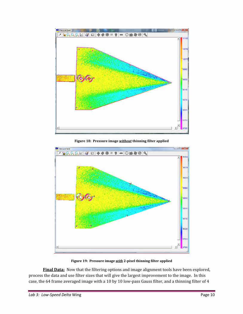
High-Pass Filters: Thinning is a high-pass filter that will clean up the edges of the image.

Use a 2 pixel filter and check the box next to ‘Thinning’. This filter will remove the given number of

pixels of bad data around the edge of the image caused by the smoothing filter. This filter can

further degrade noisy data as it is looking for edges. Notice the difference in the pressure images in

Figures 18 and 19. You can see the red line around most of the delta in Figure 18, which is due to

the low-pass filter and image misalignment. The high-pass filter and image alignment tools will

remove the line. Now we have a cleaned up image with edge effects removed. Notice also that the

effects of the physical markers (red cirles) have been removed by this filter as well.

Figure 17: Alignment and Filtering Options Panel


Figure 18: Pressure image without thinning filter applied

Figure 19: Pressure image with 2-pixel thinning filter applied

Final Data: Now that the filtering options and image alignment tools have been explored,

process the data and use filter sizes that will give the largest improvement to the image. In this

case, the 64 frame averaged image with a 10 by 10 low-pass Gauss filter, and a thinning filter of 4


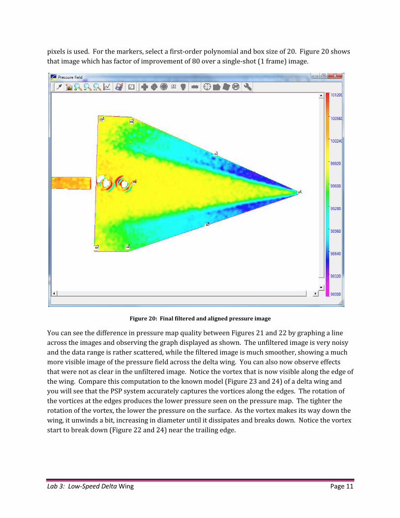
pixels is used. For the markers, select a first-order polynomial and box size of 20. Figure 20 shows

that image which has factor of improvement of 80 over a single-shot (1 frame) image.

Figure 20: Final filtered and aligned pressure image

You can see the difference in pressure map quality between Figures 21 and 22 by graphing a line

across the images and observing the graph displayed as shown. The unfiltered image is very noisy

and the data range is rather scattered, while the filtered image is much smoother, showing a much

more visible image of the pressure field across the delta wing. You can also now observe effects

that were not as clear in the unfiltered image. Notice the vortex that is now visible along the edge of

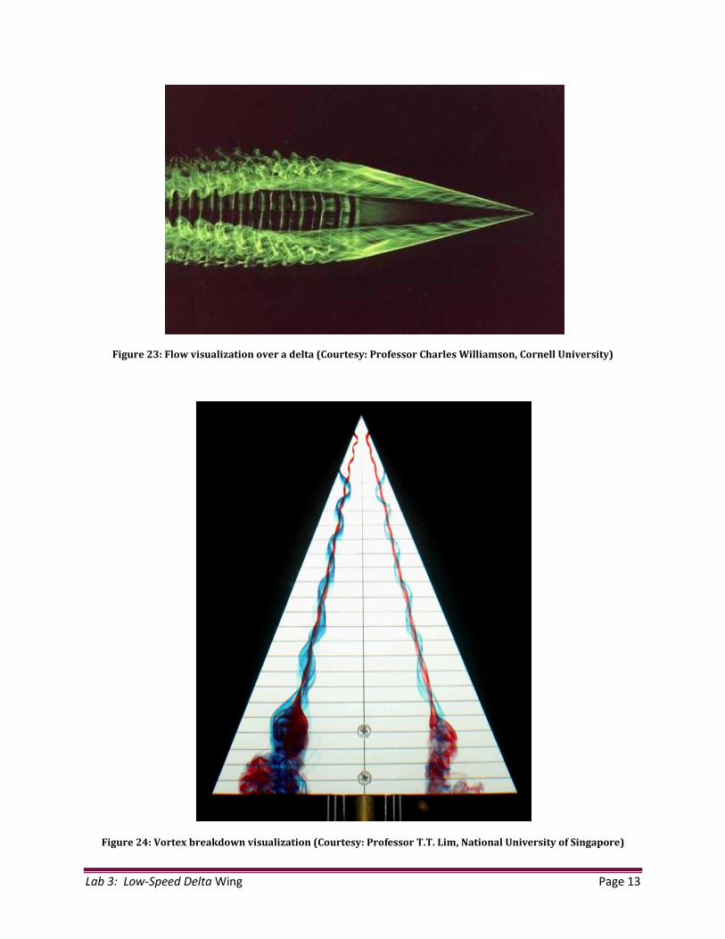
the wing. Compare this computation to the known model (Figure 23 and 24) of a delta wing and

you will see that the PSP system accurately captures the vortices along the edges. The rotation of

the vortices at the edges produces the lower pressure seen on the pressure map. The tighter the

rotation of the vortex, the lower the pressure on the surface. As the vortex makes its way down the

wing, it unwinds a bit, increasing in diameter until it dissipates and breaks down. Notice the vortex

start to break down (Figure 22 and 24) near the trailing edge.


Figure 21: Unfiltered pressure image

Figure 22: Filtered and aligned pressure image


Figure 23: Flow visualization over a delta (Courtesy: Professor Charles Williamson, Cornell University)

Figure 24: Vortex breakdown visualization (Courtesy: Professor T.T. Lim, National University of Singapore)

Lab 3: Low-Speed Delta Wing - psp-tsp.compsp-tsp.com/pdfs/Labs/Lab 3_Low Speed Delta.pdf · Lab 3:...

Documents

Transcript of Lab 3: Low-Speed Delta Wing - psp-tsp.compsp-tsp.com/pdfs/Labs/Lab 3_Low Speed Delta.pdf · Lab 3:...