Feature construction based on class

outliers

Albrecht Zimmermann

Report CW648, November 2013

KU LeuvenDepartment of Computer Science

Celestijnenlaan 200A – B-3001 Heverlee (Belgium)

Feature construction based on class

outliers

Albrecht Zimmermann

Report CW648, November 2013

Department of Computer Science, KU Leuven

Abstract

Data for training a classification model can be considered to con-sist of two types of points: easy to classify ones typical for a classand difficult to classify ones atypical for a class and often lying onclass boundaries. Most existing techniques deal with atypical pointsin later stages of model building, after typical points have been mod-eled. This means that atypical points are often modeled only if doingso results in an improvement in comparison to the model of typicalpoints. An alternative way of viewing atypical points is as outliersw.r.t. the class to which they supposedly belong. Based on this real-ization, we introduce the concept of class outliers, whose immediateneighborhoods we use to construct discriminative features. We in-vestigate ways of employing the newly derived features and comparethe quality of resulting models with results on un-augmented datafor a variety of UCI benchmarks sets. We find that while some over-fitting control can be necessary, the newly derived features improvethe classification accuracy of SVM, Naive Bayes, and C4.5 classifiers.

CR Subject Classification : I.2, H.2.8

Feature Construction based on Class Outliers

Albrecht Zimmermannalbrecht.zimmermann@cs.kuleuven.be

KU Leuven, Belgium

Abstract. Data for training a classification model can be considered toconsist of two types of points: easy to classify ones – typical for a class –and difficult to classify ones – atypical for a class and often lying on classboundaries. Most existing techniques deal with atypical points in laterstages of model building, after typical points have been modeled. Thismeans that atypical points are often modeled only if doing so resultsin an improvement in comparison to the model of typical points. Analternative way of viewing atypical points is as outliers w.r.t. the classto which they supposedly belong. Based on this realization, we introducethe concept of class outliers, whose immediate neighborhoods we use toconstruct discriminative features. We investigate ways of employing thenewly derived features and compare the quality of resulting models withresults on un-augmented data for a variety of UCI benchmarks sets.

We find that while some overfitting control can be necessary, the newlyderived features improve the classification accuracy of SVM, Naive Bayes,and C4.5 classifiers.

Keywords: feature construction, classification, outlier detection

1 Introduction

Supervised learning, the other contender being clustering, is arguably the old-est sub-discipline of machine learning. Especially in real-life data one can oftenconsider a class to consist of two types of instances. There are typical ones, i.e.representatives of the generating process, that are easy to classify since theymake up the majority of a class which allows for good generalization. On theother hand there can be atypical instances, a minority that is structurally dis-similar to the majority of the class and often prove more difficult to classify.The latter is especially then the case if these atypical instances occupy similarregions as, i.e. are similar to, instances from other classes.

The problem is well-known and has for instance been used to characterizedata sets’ learnability [9, 12] or make analytic statements about learners’ abilityto generalize from data. Additionally, all successful learning paradigms have amechanism for addressing this problem, whether by first learning the majoritymodel and modeling atypical instances if need be [4, 10, 11] or by using atypicalinstances to delineate class boundaries, modeling typical instances along the way[5].

A different way of describing atypical instances is as outliers within their as-signed class. Clustering, the “other” well-established sub-field of machine learn-ing, has had need to address outliers that cannot be assigned to any clusterseasily, eventually giving rise to outlier detection [2]. It seems therefore plausibleto employ outlier detection for identifying atypical instances and it is surprisinghow little attention has been given to exploiting the aforementioned structuraldifferences among instances of the same class. A notable exception is [13] whichused clustering to partition classes into clearly delineated sub-classes. Clusteringis concerned with uncovering the underlying structure of a data set, an aspectthat Vilalta et al.’s work exploited to create classes that are easier to model.

Our contribution is two-fold:

1. Based on this observation, we propose the concept of class outliers, i.e. in-stances of a given class that do not belong to any cluster within this class.

2. By mining discriminative patterns from the neighborhoods of such outlierswe can construct features that add additional dimensions to the descrip-tion of the data and improve class separation and hence learnability andclassification accuracy, as show experimentally

The paper is structured as follows: in the next section we introduce our notionof class outliers and discuss how to leverage them for feature generation. InSection 3, we discuss existing techniques that address atypical instances to placeour approach in context. In Section 4 we evaluate our framework experimentallyon a variety of UCI data sets, discussing resulting classification accuracies indetail, before we conclude.

2 Problem Setting and Proposed Solution

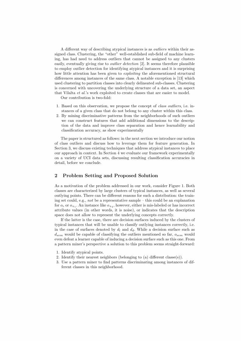
As a motivation of the problem addressed in our work, consider Figure 1. Bothclasses are characterized by large clusters of typical instances, as well as severaloutlying points. There can be different reasons for such a distribution: the train-ing set could, e.g., not be a representative sample – this could be an explanationfor o◦ or o+1 . An instance like o+2 , however, either is mis-labeled or has incorrectattribute values (in other words, it is noise), or indicates that the descriptionspace does not allow to represent the underlying concepts correctly.

If the latter is the case, there are decision surfaces induced by the clusters oftypical instances that will be unable to classify outlying instances correctly, i.e.in the case of surfaces denoted by dl and dd. While a decision surface such asdsvm would be capable of classifying the outliers mentioned so far, osvm wouldeven defeat a learner capable of inducing a decision surface such as this one. Froma pattern miner’s perspective a solution to this problem seems straight-forward:

1. Identify atypical points.2. Identify their nearest neighbors (belonging to (a) different classe(s)).3. Use a pattern miner to find patterns discriminating among instances of dif-

ferent classes in this neighborhood.

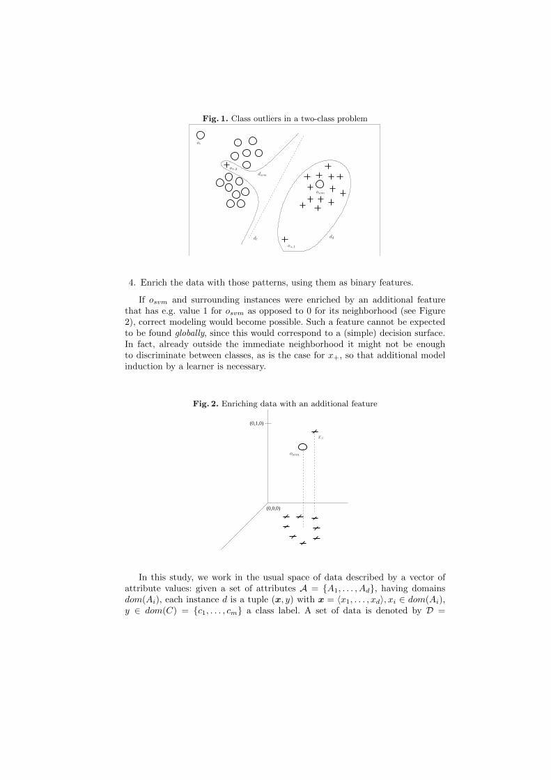
Fig. 1. Class outliers in a two-class problem

dd

o◦

o+,1

o+,2

osvm

dl

dsvm

4. Enrich the data with those patterns, using them as binary features.

If osvm and surrounding instances were enriched by an additional featurethat has e.g. value 1 for osvm as opposed to 0 for its neighborhood (see Figure2), correct modeling would become possible. Such a feature cannot be expectedto be found globally, since this would correspond to a (simple) decision surface.In fact, already outside the immediate neighborhood it might not be enoughto discriminate between classes, as is the case for x+, so that additional modelinduction by a learner is necessary.

Fig. 2. Enriching data with an additional feature

(0,1,0)

(0,0,0)

x+

osvm

In this study, we work in the usual space of data described by a vector ofattribute values: given a set of attributes A = {A1, . . . , Ad}, having domainsdom(Ai), each instance d is a tuple (x, y) with x = ⟨x1, . . . , xd⟩, xi ∈ dom(Ai),y ∈ dom(C) = {c1, . . . , cm} a class label. A set of data is denoted by D =

{d1, . . . , dn} and each class within this data set by Dc = {d = (x, y) | y = c}.A natural choice for the kind of binary feature with which to enrich the data isthe class of conjunctive patterns.1

Assuming an outlier oracle OO(d,D′) 7→ {true, false} that can decide whethera instance d is an outlier w.r.t. D′, we can define the set of class outliers:

Definition 1 Given a set of labeled data D = {(x, y)}, the set of outliers ofclass c in D is defined as Oc,D = {d ∈ Dc | OO(d,Dc) = true}. The union overall the outliers of all classes OC,D =

∪c Oc,D is called the set of class outliers.

For each instance d, we can define its k-neighborhood, i.e. the k instances inD that are closest to d:

Definition 2 Given an instance d and a distance measure δ : D × D 7→ R,its k-neighborhood is defined as: Nk(d) = {d′ ∈ D \ {d} s.t. |{d′′ | δ(d′′, d) ≤δ(d′, d)}| ≤ k − 1}

By assembling the k-neighborhoods of all class outliers in D, we are select-ing small subsets where local decision boundaries can be expected to occur. Wefurthermore assume a pattern miner PM(D) capable of constructing discrimi-native patterns from a multi-class data set. Such a pattern miner can take theform of a class-association rule miner but also a regular learner for classificationrules or a decision tree learner. Using it we construct patterns from the respec-tive Nk(o), e.g. the left-hand sides of predictive rules, which we can then use toenrich the data. A high-level algorithm summarizing the steps involved in ourfeature construction approach is given as Algorithm 1.

If all instances in a k-neighborhood belong to the same class as the outlieritself, the outlier that gave rise to it was atypical but not hard to classify, andwe therefore ignore the subset for the purpose of feature construction (line 9).Furthermore, it is possible that the k-neighborhood of a class outlier includesone (or several) other class outlier(s). Since using these subsets separately wouldprobably give rise to a number of redundant features, we instead merge any pairof k-neighborhoods of class outliers whose intersection includes at least 50%of the instances of the smaller neighborhood (lines 12/13). Note, that this is atransitive relationship. Once all such neighborhoods have been identified, we canuse the pattern miner to derive features for augmenting the data.

This augmentation takes the form that we add one binary attribute perpattern to each instance, with the value 1 if the pattern matches the instanceand the value 0 if it does not.

1 While we limit ourselves to the space of attribute-valued data herein, this is w.l.o.g.Any instance space in which a distance measure between instances is defined allowsfor the identification of outliers, as well as each instance space that allows for patternmining operations allows to derive features from these outliers.

Algorithm 1 High-level algorithm for class outlier-based feature construction

1: Given: data set D, set of class labels C2: Return: set of discriminative patterns F3:4: OC,D = ∅5: for c ∈ C do6: OC,D = OC,D ∪ Oc,D7: N = ∅8: for o ∈ OC,D do9: if ∃di = (xi, yi), dj = (xj , yj) ∈ Nk(o) : yi = yj then

10: N = N ∪ {Nk(o)}11: while ∃Nk(o), Nk(o′) ∈ N : (o ∈ Nk(o′) ∨ o′ ∈ Nk(o)) ∧ |Nk(o′)∩Nk(o)|

min{|Nk(o′)|,|Nk(o)|} ≥ 0.5do

12: Nk(o′) = Nk(o′) ∪ Nk(o)13: for Nk(o) ∈ N do14: F = F∪ {PM(Nk(o))}15: return F

3 Related Work

The problem of atypical instances has of course been identified early on in clas-sification learning and some way of dealing with it is included in most learningtechniques.

Decision trees [10], are induced in such a manner that subsets with lowclass-entropy are split off while deepening the tree, ideally ones that have highcardinality. Deeper nodes in the tree then consist of hard-to-separate, i.e. atyp-ical, instances of which smaller subsets are split off. In the case of sequentialrule learning [4], on the other hand, this is achieved by sequential covering tech-niques that typically learn rules of high accuracy early on, remove the coveredinstances, which are typical of one of the classes, until only data from boundaryregions remains for which then rules are learned that often have lower accuracy.Rule learning can also be employed in a second mode, in which rules do notform a sequential list derived by sequential covering, but an unordered set. Forunseen instances, all rules are selected that match the instances and called uponto make a decision. For atypical instances, this can lead to conflicting predic-tions which are then integrated using a voting mechanism. The authors of [8]go beyond this by collecting all instances covered by conflicting rules, i.e. atyp-ical instances, and reinducing classification rules on this subset. Boosting [11]also follows a strategy of modeling typical instances first. After inducing a firstmodel, misclassified instances are given larger weight for the next modeling step.Depending on the choice of weak learner, this can lead to modeling of typicalinstances from different classes in turn, before atypical instances are modeled.

All those techniques work by modeling typical instances first and then mod-eling atypical instances in the context of these prior models. Therefore, partialmodels for typical instances may include some misclassified atypical instanceswhose error is marginalized by the correct prediction on the typical ones. Addi-

tionally, attempts to avoid over-fitting can lead to pruning of the rules and testsreferring to atypical instances, losing the ability to classify them correctly. Ourproposed approach instead treats atypical instances first and augments typicalinstances in terms of found patterns.

In contrast, Support Vector Machines (SVM) [5] in a sense focus on atypicalinstances: in SVM learning, a separating hyperplane between two classes is foundthat maximizes the distance to the closest instances (support vectors) of eachclass. Support vectors, lying on class boundaries, may be atypical instances that,if modeled correctly, enable the classification of typical ones. Since the separatinghyperplane is constructed globally, however, atypical points have to be accom-modated globally as well, potentially leading to rather complex hyperplanes, e.g.for o+,2 in Figure 1. To control over-fitting, the complexity of the hyperplane istypically traded off against the errors committed in classification, meaning thatmodeling of atypical instances may be sacrificed again if enough typical onesare modeled correctly. Contrary to this, our proposed approach treats atypicalinstances in a local context, reducing the strain on the global model.

Additionally, there are k-NN classifiers [6] and related techniques such aslocally weighted regression [3] that use the k-neighborhood of an instance forclassification. An obvious difference to our approach lies in that k-nearest neigh-bor techniques use the neighborhood to assign a label to the instance, thereforepotentially exacerbating the situation in the case of class outliers, while we useit to construct discriminating features.

There have been works characterizing the difficulty of learning problems interms of direct neighbors in the description space having differing class labels,via class variation [9]. Since the original definition of class variation was limitedto binary vectors and neighbors that differ in at most one attribute value, it wasgeneralized in [12] to a distance-based notion that compares the class labels ofinstances within a certain radius around a given instance. Both of these works,however, do not attempt to exploit knowledge about neighbors with differingclass labels to aid classification. Such a step was taken in [13], in which clusteringis used to explain Naıve Bayes well-known good performance, and to partitionclasses with difficult structure into subclusters to improve classification accuracy.

Generally speaking, the treatment of atypical instances has been somewhatdifferent in the context of clustering and outlier detection. In clustering, instancesthat do not fit any of the formed clusters are often removed from the data withthe goal of producing well-described clusters. Those outliers are usually eitherconsidered noise or to form their own (minority) clusters. Outlier detection,e.g. [2], finally, assumes that outliers are abnormalities that carry importantinformation and treats them not as an unwanted side-product but as the maintarget of data mining.

4 Experimental Setup

We expect the class outlier-derived features to help improve the modeling ofclassification problems and therefore the estimated classification accuracy. To

evaluate classification performance, we perform a ten-fold cross-validation on anumber of UCI data sets [1]. We aimed at data sets of different dimensionality,different size, and different distribution and number of classes to allow us toevaluate the behavior of class outlier detection and the effects of derived fea-tures thoroughly.2 For each fold, class outliers and their k-neighborhoods areextracted from the combined training folds, and conjunctive patterns mined onthese subsets. As learners we used the SVM implementation contained in theWEKA workbench [7], as well as the J48 decision tree and the Naıve Bayesclassifiers. As to the two components of our approach, the outlier oracle and thepattern miner:

– To identify class outliers, we use the LOF algorithm proposed in [2] in theversion available for download by the authors as part of the ELKI package.3

– To mine conjunctive patterns, we use the C4.5 implementation of WEKA,with pruning turned off and minimum number of instances set to 1. Wetransform the resulting tree into conjunctive rules and use the left-hand sideof these rules as features for augmentation.

4.1 Outlier Detection

LOF is a distance-based approach that calculates a local outlier factor (lof )by comparing the distance of an instance d to points in its k-neighborhood tothe average distance of points within Nk(d). The local outlier factor is thereforestrongly dependent on k: lof k(d) (and the data set on which it is derived, omittedfrom the notation). In combination with a threshold lmin, the outlier oracle takesthe form: OO(d,Dc) := lof k(d) ≥ lmin

We chose Euclidean distance for data with numerical attributes and Manhat-tan distance for nominally valued data. To use the Manhattan distance, nominalattributes were binarized into a number of binary-valued attributes.

The decision on the size of the k-neighborhood is not straight-forward. Toget a reliable estimate, the authors of LOF recommend to calculate a number oflof over an interval [kmin, kmax]. An additional recommendation is to set k ≥ 10to remove statistical fluctuations. Since this is not always possible, especiallyfor small classes, we instead based our choice of the minimum k-value on thefollowing considerations:

– We assume that the minimum size k-neighborhood for a point can be 10%of the class.

– If these 10% are larger than ten, we follow the advice of the authors of LOFand set kmin to ten.

– The minimum number of k needed to derive a meaningful outlier is two,so this is set as a hard minimum and if a class does not support a 2-neighborhood for a given point, no outlier calculation is performed.

2 We do not list their characteristics since those can be accessed at the UCI repository.3 At: http://www.dbs.ifi.lmu.de/research/KDD/ELKI/

To summarize: kmin(Dc) = max{2, min{10, |Dc|10 }}. Second, the authors of [2]

state that maximum k should be ”...the maximum number of ’close’ by objectsthat can potentially be local outliers.” We use the following heuristics for select-ing a maximum k:

– At most 50% of the class can be local outliers since otherwise the concept ofa distinct “class” becomes questionable.

– To facilitate termination, we initially limit kmax to twenty.– It turns out, however, that for k = 20 occasionally points receive an outlier

factor of ”NaN” or ∞. We therefore increment kmax until there is at leastone numeric lof value for each point of a class.

Thus: kmax(Dc) = max{{k s.t. ∀d ∈ Dc : lofk(d) ∈ R},min{20, |Dc|2 }}. Table 1

gives an impression of the range of k-values for different data sets and classes. Itreports all [kmin, kmax] intervals used for different classes of a data set, annotatedwith the number of classes for which this interval was used. The table shows thatmany classes are not large enough to allow for 10 instances involved in the lof -calculation but also that 20 is often a sufficiently large kmax-value to derive alof -value for all instances of a class.

This procedure gives rise to a set of local outlier factors for each point andthe question remains how to interpret those. Generally speaking, a local outlierfactor larger than 1 indicates an outlier. According to [2], the best way to decidewhether a point is in fact an outlier consists of taking the maximum lof valueover the entire range of k. The rationale for this is that using the average outlierfactor might lead to its being an outlier being overridden by the effects of havinganother local outlier in the neighborhood.

As illustration, consider Figure 3. In the case of k = 2, the two neighbors ofthe instance in question are much easier to reach, and the instance is assigneda high lof. If k is increased to 3, however, the third neighbor is a local outlieritself, harder to reach and therefore makes the instance in question appear more“normal”. Using the maximum outlier factor and a threshold of 1 to decide onwhether instances are outliers leads to an excessive amount of instances perclass tagged as outliers, as Figure 4 shows. The values reported are the weightedaverage over all classes, i.e. each class’ contribution to the overall average valueis weighted by its proportional size.

In fact, even using the average outlier factor and threshold 1, i.e. using anoracle of the form:

OOavg(d,Dc) :=

∑kmax(Dc)k=kmin(Dc)

lof k(d)

kmax(Dc) − kmin(Dc)> 1,

leads to more than half of all instances being tagged as outliers (cf. Figure4). Clearly, using a threshold of 1 to identify class outliers is overly strict. Inreaction to this, we evaluated a number of different thresholds in the range[1, 3] with increments of 0.0625. Thresholds and selection methods have beenchosen for each class separately since differing underlying distributions can leadto differing outlier behavior. The goal was to find the largest set of outliers that

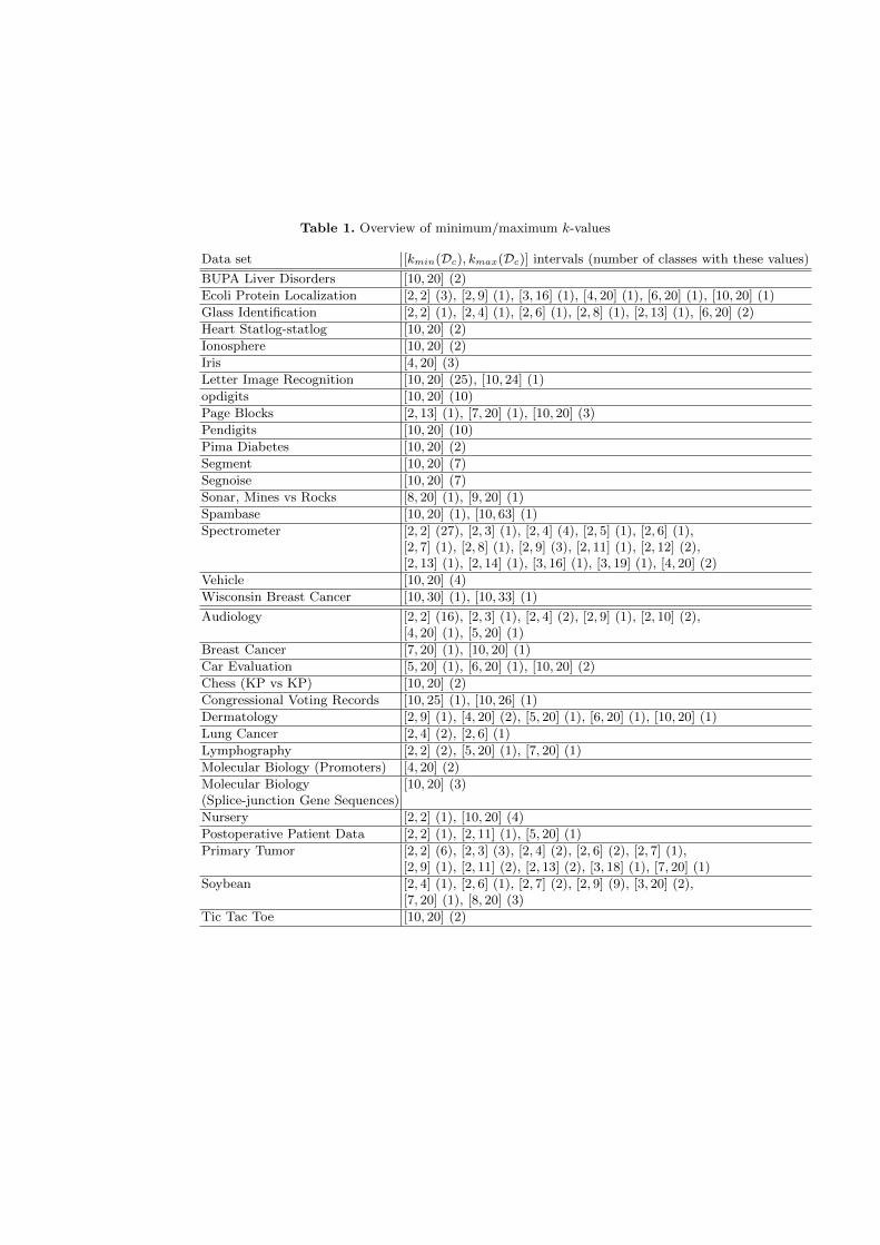
Table 1. Overview of minimum/maximum k-values

Data set [kmin(Dc), kmax(Dc)] intervals (number of classes with these values)

BUPA Liver Disorders [10, 20] (2)

Ecoli Protein Localization [2, 2] (3), [2, 9] (1), [3, 16] (1), [4, 20] (1), [6, 20] (1), [10, 20] (1)

Glass Identification [2, 2] (1), [2, 4] (1), [2, 6] (1), [2, 8] (1), [2, 13] (1), [6, 20] (2)

Heart Statlog-statlog [10, 20] (2)

Ionosphere [10, 20] (2)

Iris [4, 20] (3)

Letter Image Recognition [10, 20] (25), [10, 24] (1)

opdigits [10, 20] (10)

Page Blocks [2, 13] (1), [7, 20] (1), [10, 20] (3)

Pendigits [10, 20] (10)

Pima Diabetes [10, 20] (2)

Segment [10, 20] (7)

Segnoise [10, 20] (7)

Sonar, Mines vs Rocks [8, 20] (1), [9, 20] (1)

Spambase [10, 20] (1), [10, 63] (1)

Spectrometer [2, 2] (27), [2, 3] (1), [2, 4] (4), [2, 5] (1), [2, 6] (1),[2, 7] (1), [2, 8] (1), [2, 9] (3), [2, 11] (1), [2, 12] (2),[2, 13] (1), [2, 14] (1), [3, 16] (1), [3, 19] (1), [4, 20] (2)

Vehicle [10, 20] (4)

Wisconsin Breast Cancer [10, 30] (1), [10, 33] (1)

Audiology [2, 2] (16), [2, 3] (1), [2, 4] (2), [2, 9] (1), [2, 10] (2),[4, 20] (1), [5, 20] (1)

Breast Cancer [7, 20] (1), [10, 20] (1)

Car Evaluation [5, 20] (1), [6, 20] (1), [10, 20] (2)

Chess (KP vs KP) [10, 20] (2)

Congressional Voting Records [10, 25] (1), [10, 26] (1)

Dermatology [2, 9] (1), [4, 20] (2), [5, 20] (1), [6, 20] (1), [10, 20] (1)

Lung Cancer [2, 4] (2), [2, 6] (1)

Lymphography [2, 2] (2), [5, 20] (1), [7, 20] (1)

Molecular Biology (Promoters) [4, 20] (2)

Molecular Biology [10, 20] (3)(Splice-junction Gene Sequences)

Nursery [2, 2] (1), [10, 20] (4)

Postoperative Patient Data [2, 2] (1), [2, 11] (1), [5, 20] (1)

Primary Tumor [2, 2] (6), [2, 3] (3), [2, 4] (2), [2, 6] (2), [2, 7] (1),[2, 9] (1), [2, 11] (2), [2, 13] (2), [3, 18] (1), [7, 20] (1)

Soybean [2, 4] (1), [2, 6] (1), [2, 7] (2), [2, 9] (9), [3, 20] (2),[7, 20] (1), [8, 20] (3)

Tic Tac Toe [10, 20] (2)

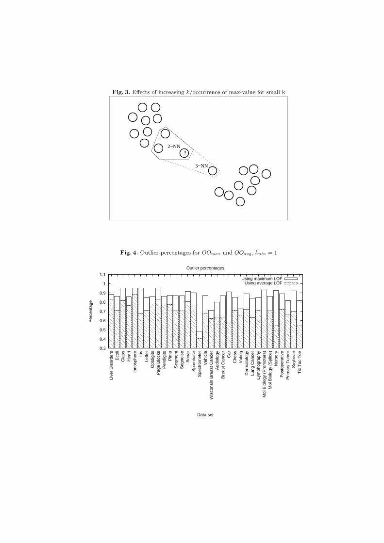
Fig. 3. Effects of increasing k/occurrence of max-value for small k

3−NN

2−NN?

Fig. 4. Outlier percentages for OOmax and OOavg, lmin = 1

0.3

0.4

0.5

0.6

0.7

0.8

0.9

1

1.1

Live

r D

isor

ders

Eco

liG

lass

Hea

rtIo

nosp

here Iris

Lette

rO

ptdi

gits

Pag

e B

lock

sP

endi

gits

Pim

aS

egm

ent

Seg

nois

eS

onar

Spa

mba

seS

pect

rom

eter

Veh

icle

Wis

cons

in B

reas

t Can

cer

Aud

iolo

gyB

reas

t Can

cer

Car

Che

ssV

otin

gD

erm

atol

ogy

Lung

Can

cer

Lym

phog

raph

yM

ol B

iolo

gy (

Pro

mot

ers)

Mol

Bio

logy

(S

plic

e)N

urse

ryP

osto

pera

tive

Prim

ary

Tum

orS

oybe

anT

ic T

ac T

oe

Per

cent

age

Data set

Outlier percentages

Using maximum LOFUsing average LOF

did not exceed 10% of a class’ instances. A summary of the chosen threshold-values and selection methods for different classes and data sets is given in Table2. Averaging thresholds over different classes does not give a comprehensiblepicture so we chose the same presentation as in the case of [kmin, kmax] intervals.

The results show that there is no one setting that can be applied to all classesin a data set, let alone across different data sets. Due to different underlyingdistributions instances whose lof would tag them as outliers in one class mightbe considered average instances in another class.

4.2 Feature Construction

Once the class outliers are identified, it is necessary to decide on the k parameterused to assemble each outliers’ k-neighborhood. Given the results of selecting k-values for calculating the lof -score, we decided against setting a single k for allclasses of a data set. Instead, we use the information about the selection methodused to decide that an instance is an outlier for guidance:

– If o was tagged as an outlier using OOmax, we use the k for which lof k(o) ismaximal

– If o was tagged as an outlier using OOavg, we use the average over all k forwhich lof k(o) ∈ R

The important difference to the outlier detection step lies in the fact thatduring outlier detection k instances from the same class as o are used while forfeature construction all classes are involved in selecting the k nearest neighbors.

We use the WEKA-implementation of C4.5 to derive the conjunctive pat-terns. Since the subsets are relatively small and not representative of the dis-tribution of the entire data set, we do not perform any pruning of the resultingdecision trees and set the minimum number of instances per leaf to 1. We donot attempt to address over-fitting in this step but instead rely on the learner’sregularization mechanism.

When gathering the features derived from each subset into a complete featureset, it is possible that a single pattern might predict different classes, dependingon the subset from which they were constructed. Since this indicates that thesefeatures lack the ability to discriminate classes, we remove them from the set.

4.3 Experimental Evaluation: Classification Accuracy

We chose the RBF kernel (with standard WEKA settings) for the SVM classifierand selected the C-parameter by internal five-fold cross-validation from the range[1, 128], doubling the value in each step. The SVM-implementation contained inWEKA took more than 24 hours for a single fold of the Letter data set, leading usto remove it from the SVM’s evaluation. J48 and Naıve Bayes were run using thestandard settings predefined in WEKA. We show the resulting accuracies for theSVM in table 3, and the results for J48 and Naıve Bayes in 4. The tables alwayslist both the training and testing accuracy for the original representation and

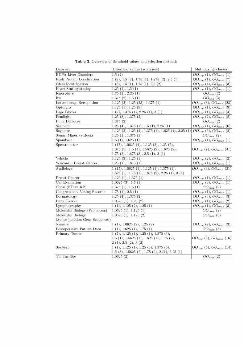
Table 2. Overview of threshold values and selection methods

Data set Threshold values (# classes) Methods (# classes)

BUPA Liver Disorders 1.5 (2) OOavg (1), OOmax (1)

Ecoli Protein Localization 1 (2), 1.5 (2), 1.75 (1), 1.875 (2), 2.5 (1) OOavg (1), OOmax (7)

Glass Identification 1 (3), 1.5 (1), 1.75 (1), 2.5 (2) OOavg (4), OOmax (3)

Heart Statlog-statlog 1.25 (1), 1.5 (1) OOavg (1), OOmax (1)

Ionosphere 1.75 (1), 2.25 (1) OOavg (2)

Iris 1.375 (2), 1.5 (1) OOavg (3)

Letter Image Recognition 1.125 (2), 1.25 (23), 1.375 (1) OOavg (3), OOmax (23)

Optdigits 1.125 (1), 1.25 (9) OOavg (1), OOmax (9)

Page Blocks 1 (2), 1.375 (1), 2.25 (1), 3 (1) OOavg (1), OOmax (4)

Pendigits 1.25 (8), 1.375 (2) OOavg (2), OOmax (8)

Pima Diabetes 1.375 (2) OOavg (2)

Segment 1.25 (4), 1.375 (1), 1.5 (1), 2.25 (1) OOavg (1), OOmax (6)

Segnoise 1.125 (2), 1.25 (2), 1.375 (1), 1.625 (1), 2.25 (1) OOavg (5), OOmax (2)

Sonar, Mines vs Rocks 1.25 (1), 1.375 (1) OOmax (2)

Spambase 1.5 (1), 1.625 (1) OOavg (1), OOmax (1)

Spectrometer 1 (17), 1.0625 (4), 1.125 (2), 1.25 (5),1.375 (5), 1.5 (4), 1.5625 (2), 1.625 (2), OOavg (7), OOmax (41)1.75 (2), 1.875 (3), 2.5 (1), 3 (1)

Vehicle 1.125 (3), 1.25 (1) OOavg (2), OOmax (2)

Wisconsin Breast Cancer 1.25 (1), 1.875 (1) OOavg (1), OOmax (1)

Audiology 1 (15), 1.0625 (1), 1.125 (1), 1.375 (1), OOavg (3), OOmax (21)1.625 (1), 1.75 (1), 1.875 (2), 2.25 (1), 3 (1)

Breast-Cancer 1.125 (1), 1.375 (1) OOavg (1), OOmax (1)

Car Evaluation 1.0625 (3), 1.5 (1) OOavg (3), OOmax (1)

Chess (KP vs KP) 1.375 (1), 1.5 (1) OOmax (2)

Congressional Voting Records 1.75 (1), 2.5 (1) OOavg (1), OOmax (1)

Dermatology 1.25 (4), 1.375 (2) OOavg (3), OOmax (3)

Lung Cancer 1.0625 (1), 1.25 (2) OOavg (1), OOmax (2)

Lymphography 1 (1), 1.125 (2), 1.25 (1) OOavg (1), OOmax (3)

Molecular Biology (Promoters) 1.0625 (1), 1.125 (1) OOmax (2)

Molecular Biology 1.0625 (1), 1.125 (2) OOmax (3)(Splice-junction Gene Sequences)

Nursery 1 (1), 1.0625 (2), 1.25 (2) OOavg (2), OOmax (3)

Postoperative Patient Data 1 (1), 1.625 (1), 1.75 (1) OOmax (3)

Primary Tumor 1 (7), 1.125 (1), 1.25 (1), 1.375 (3),1.5 (1), 1.5625 (1), 1.625 (1), 1.75 (2), OOavg (6), OOmax (16)2 (1), 2.5 (2), 3 (2)

Soybean 1 (1), 1.125 (1), 1.25 (3), 1.375 (5), OOavg (5), OOmax (14)1.5 (3), 1.5625 (2), 1.75 (2), 2 (1), 2.25 (1)

Tic Tac Toe 1.0625 (2) OOavg (2)

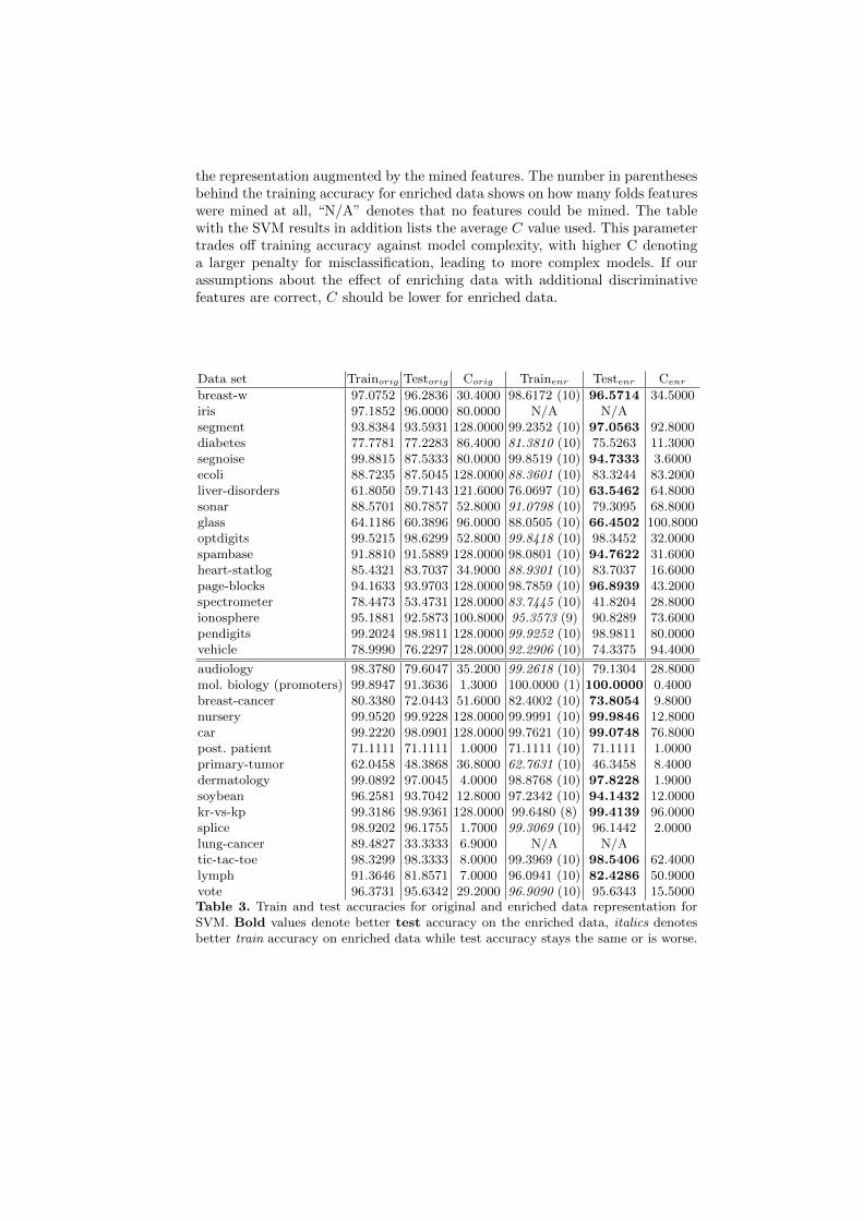
the representation augmented by the mined features. The number in parenthesesbehind the training accuracy for enriched data shows on how many folds featureswere mined at all, “N/A” denotes that no features could be mined. The tablewith the SVM results in addition lists the average C value used. This parametertrades off training accuracy against model complexity, with higher C denotinga larger penalty for misclassification, leading to more complex models. If ourassumptions about the effect of enriching data with additional discriminativefeatures are correct, C should be lower for enriched data.

Data set Trainorig Testorig Corig Trainenr Testenr Cenr

breast-w 97.0752 96.2836 30.4000 98.6172 (10) 96.5714 34.5000iris 97.1852 96.0000 80.0000 N/A N/Asegment 93.8384 93.5931 128.0000 99.2352 (10) 97.0563 92.8000diabetes 77.7781 77.2283 86.4000 81.3810 (10) 75.5263 11.3000segnoise 99.8815 87.5333 80.0000 99.8519 (10) 94.7333 3.6000ecoli 88.7235 87.5045 128.0000 88.3601 (10) 83.3244 83.2000liver-disorders 61.8050 59.7143 121.6000 76.0697 (10) 63.5462 64.8000sonar 88.5701 80.7857 52.8000 91.0798 (10) 79.3095 68.8000glass 64.1186 60.3896 96.0000 88.0505 (10) 66.4502 100.8000optdigits 99.5215 98.6299 52.8000 99.8418 (10) 98.3452 32.0000spambase 91.8810 91.5889 128.0000 98.0801 (10) 94.7622 31.6000heart-statlog 85.4321 83.7037 34.9000 88.9301 (10) 83.7037 16.6000page-blocks 94.1633 93.9703 128.0000 98.7859 (10) 96.8939 43.2000spectrometer 78.4473 53.4731 128.0000 83.7445 (10) 41.8204 28.8000ionosphere 95.1881 92.5873 100.8000 95.3573 (9) 90.8289 73.6000pendigits 99.2024 98.9811 128.0000 99.9252 (10) 98.9811 80.0000vehicle 78.9990 76.2297 128.0000 92.2906 (10) 74.3375 94.4000

audiology 98.3780 79.6047 35.2000 99.2618 (10) 79.1304 28.8000mol. biology (promoters) 99.8947 91.3636 1.3000 100.0000 (1) 100.0000 0.4000breast-cancer 80.3380 72.0443 51.6000 82.4002 (10) 73.8054 9.8000nursery 99.9520 99.9228 128.0000 99.9991 (10) 99.9846 12.8000car 99.2220 98.0901 128.0000 99.7621 (10) 99.0748 76.8000post. patient 71.1111 71.1111 1.0000 71.1111 (10) 71.1111 1.0000primary-tumor 62.0458 48.3868 36.8000 62.7631 (10) 46.3458 8.4000dermatology 99.0892 97.0045 4.0000 98.8768 (10) 97.8228 1.9000soybean 96.2581 93.7042 12.8000 97.2342 (10) 94.1432 12.0000kr-vs-kp 99.3186 98.9361 128.0000 99.6480 (8) 99.4139 96.0000splice 98.9202 96.1755 1.7000 99.3069 (10) 96.1442 2.0000lung-cancer 89.4827 33.3333 6.9000 N/A N/Atic-tac-toe 98.3299 98.3333 8.0000 99.3969 (10) 98.5406 62.4000lymph 91.3646 81.8571 7.0000 96.0941 (10) 82.4286 50.9000vote 96.3731 95.6342 29.2000 96.9090 (10) 95.6343 15.5000Table 3. Train and test accuracies for original and enriched data representation forSVM. Bold values denote better test accuracy on the enriched data, italics denotesbetter train accuracy on enriched data while test accuracy stays the same or is worse.

It can be seen that all learners profit from the new representation on a numberof data sets (denoted in bold), sometimes dramatically so, as in the case ofSegnoise for the SVM, Molecular Biology (Promoters) for J48, or Glass andVehicle for Naıve Bayes. We can also see that on the majority of data sets,C decreases for the enriched representation, indicating that decision surfacesbecome easier to model for the SVM. On the other hand, there are a numberof data sets where the test accuracy does not change or even becomes worse,while the training accuracy on the enriched representation increases (denoted initalics). This strongly implies overfitting effects.

J48 Naıve BayesData set Trainorig Testorig Trainenr Testenr Trainorig Testorig Trainenr Testenr

breast-w 97.8541 94.2836 97.9018 (10) 96.1429 96.0420 95.9979 96.7891 96.7143iris 98.0000 94.0000 N/A N/A 95.8519 96.0000 N/A N/Asegment 99.1390 96.5368 98.9033 (10) 96.6667 80.4858 80.1732 89.5046 88.7446diabetes 83.4050 73.5732 90.4947 (10) 72.6572 76.2733 76.1842 74.5659 72.1514letter 96.2039 88.1900 97.0444 (10) 87.3650 64.5639 64.0900 72.7344 71.8450segnoise 99.0222 94.8667 98.4815 (10) 93.1333 81.8815 80.8667 90.6963 89.6667ecoli 93.0889 81.8360 91.5004 (10) 80.3565 88.3265 85.4278 86.4420 84.5276liver-disorders 85.5741 64.9328 89.7601 (10) 64.3025 56.8778 53.3361 67.9570 57.7059sonar 98.1306 71.1667 97.2767 (10) 70.6667 72.2764 67.8334 73.1830 68.3095glass 93.0961 66.8831 92.1602 (10) 69.2208 54.7736 47.3593 69.0045 59.3723optdigits 98.0032 90.3915 97.7778 (10) 90.8897 91.8189 91.2990 92.1313 91.9395spambase 97.1987 92.4585 97.1093 (10) 93.1322 79.7001 79.6783 88.1137 88.0027heart-statlog 92.7161 76.2963 92.0988 (10) 79.2593 85.7613 83.7037 86.7901 83.7037page-blocks 98.5850 97.0219 98.6276 (10) 96.8756 90.3100 90.2795 91.6580 91.6317spectrometer 90.5630 48.9623 88.5123 (10) 43.8854 62.0842 42.7358 66.1433 42.3585ionosphere 98.4173 90.0238 97.8899 (9) 88.6155 83.5709 82.6270 86.7043 84.4973pendigits 99.2581 96.3701 99.0245 (10) 95.9789 85.8645 85.7168 85.8887 85.7441vehicle 91.5293 74.5966 94.1951 (10) 73.0504 46.9265 45.2675 64.9719 62.8852

audiology 90.0679 77.4111 91.1004 (10) 76.0277 78.5637 71.6601 78.8093 72.0356mol. biology (prom.) 95.5965 78.3636 95.7895 (1) 90.9091 98.9507 91.4545 98.9474 100.0000breast-cancer 76.4582 75.9113 82.1692 (10) 73.4360 75.5239 72.3645 75.9523 73.0542nursery 98.1490 97.2453 99.5122 (10) 98.2099 90.3678 90.3087 93.8674 93.6960car 96.1355 92.3615 97.9810 (10) 94.0392 86.9856 85.2987 90.0592 88.5415post. patient 71.3580 68.8889 71.7284 (10) 68.8889 74.3210 68.8889 73.9506 64.4445primary-tumor 60.6683 39.5544 65.1912 (10) 40.7130 56.6375 50.1604 50.8036 41.6132dermatology 97.8750 94.5345 97.6018 (10) 92.8979 98.9981 98.3709 99.3017 98.3709soybean 96.0144 92.5362 96.3885 (10) 91.3747 93.5904 92.8261 92.8418 90.3410kr-vs-kp 99.6454 99.4685 99.5872 (8) 99.5311 88.2075 87.6406 79.4882 79.9353splice 96.2696 94.3573 97.2379 (10) 94.0439 95.8899 95.3919 94.9878 94.7649lung-cancer 86.4655 50.0000 N/A N/A 88.5222 51.6667 N/A N/Atic-tac-toe 93.7020 84.9715 96.3001 (10) 91.4364 70.6332 69.8278 75.1797 74.6327lymph 90.6913 78.3333 91.5155 (10) 77.0000 88.4390 83.9047 88.1399 83.0476vote 97.1904 96.5592 97.2670 (10) 96.3266 90.3192 89.8731 93.7172 92.4102

Table 4. Train and test accuracies for original and enriched data representation forJ48 and Naıve Bayes. Bold values denote better test accuracy on the enriched data,italics denotes better train accuracy on enriched data while test accuracy stays thesame or is worse.

Overfitting control by minimum support As a straightforward way of controllingspurious features, we therefore evaluate the effect of removing spurious featuresby requiring a minimum support of each pattern that is used as a feature. Tables5, 6, and 7 show the resulting accuracies when a minimum support of 2, 3, 4, 5,

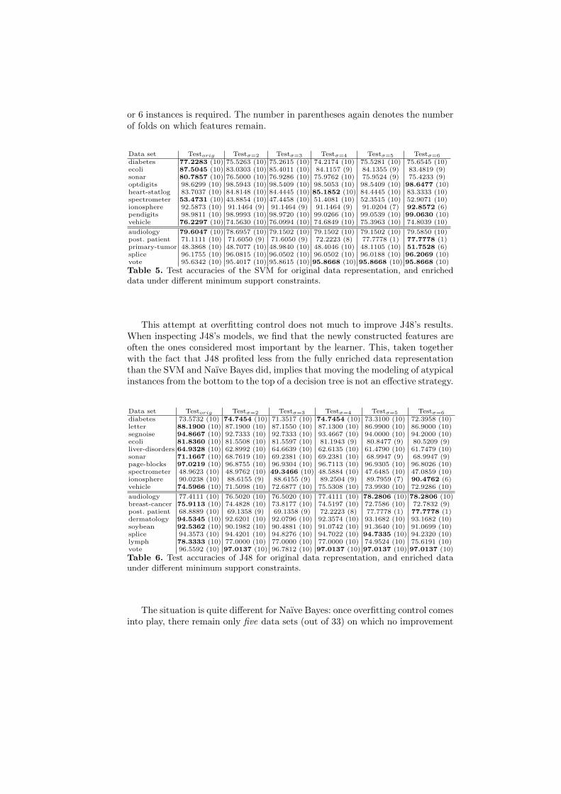
or 6 instances is required. The number in parentheses again denotes the numberof folds on which features remain.

Data set Testorig Testσ=2 Testσ=3 Testσ=4 Testσ=5 Testσ=6

diabetes 77.2283 (10) 75.5263 (10) 75.2615 (10) 74.2174 (10) 75.5281 (10) 75.6545 (10)ecoli 87.5045 (10) 83.0303 (10) 85.4011 (10) 84.1157 (9) 84.1355 (9) 83.4819 (9)sonar 80.7857 (10) 76.5000 (10) 76.9286 (10) 75.9762 (10) 75.9524 (9) 75.4233 (9)optdigits 98.6299 (10) 98.5943 (10) 98.5409 (10) 98.5053 (10) 98.5409 (10) 98.6477 (10)heart-statlog 83.7037 (10) 84.8148 (10) 84.4445 (10) 85.1852 (10) 84.4445 (10) 83.3333 (10)spectrometer 53.4731 (10) 43.8854 (10) 47.4458 (10) 51.4081 (10) 52.3515 (10) 52.9071 (10)ionosphere 92.5873 (10) 91.1464 (9) 91.1464 (9) 91.1464 (9) 91.0204 (7) 92.8572 (6)pendigits 98.9811 (10) 98.9993 (10) 98.9720 (10) 99.0266 (10) 99.0539 (10) 99.0630 (10)vehicle 76.2297 (10) 74.5630 (10) 76.0994 (10) 74.6849 (10) 75.3963 (10) 74.8039 (10)

audiology 79.6047 (10) 78.6957 (10) 79.1502 (10) 79.1502 (10) 79.1502 (10) 79.5850 (10)post. patient 71.1111 (10) 71.6050 (9) 71.6050 (9) 72.2223 (8) 77.7778 (1) 77.7778 (1)primary-tumor 48.3868 (10) 48.7077 (10) 48.9840 (10) 48.4046 (10) 48.1105 (10) 51.7528 (6)splice 96.1755 (10) 96.0815 (10) 96.0502 (10) 96.0502 (10) 96.0188 (10) 96.2069 (10)vote 95.6342 (10) 95.4017 (10) 95.8615 (10) 95.8668 (10) 95.8668 (10) 95.8668 (10)

Table 5. Test accuracies of the SVM for original data representation, and enricheddata under different minimum support constraints.

This attempt at overfitting control does not much to improve J48’s results.When inspecting J48’s models, we find that the newly constructed features areoften the ones considered most important by the learner. This, taken togetherwith the fact that J48 profited less from the fully enriched data representationthan the SVM and Naıve Bayes did, implies that moving the modeling of atypicalinstances from the bottom to the top of a decision tree is not an effective strategy.

Data set Testorig Testσ=2 Testσ=3 Testσ=4 Testσ=5 Testσ=6

diabetes 73.5732 (10) 74.7454 (10) 71.3517 (10) 74.7454 (10) 73.3100 (10) 72.3958 (10)letter 88.1900 (10) 87.1900 (10) 87.1550 (10) 87.1300 (10) 86.9900 (10) 86.9000 (10)segnoise 94.8667 (10) 92.7333 (10) 92.7333 (10) 93.4667 (10) 94.0000 (10) 94.2000 (10)ecoli 81.8360 (10) 81.5508 (10) 81.5597 (10) 81.1943 (9) 80.8477 (9) 80.5209 (9)liver-disorders 64.9328 (10) 62.8992 (10) 64.6639 (10) 62.6135 (10) 61.4790 (10) 61.7479 (10)sonar 71.1667 (10) 68.7619 (10) 69.2381 (10) 69.2381 (10) 68.9947 (9) 68.9947 (9)page-blocks 97.0219 (10) 96.8755 (10) 96.9304 (10) 96.7113 (10) 96.9305 (10) 96.8026 (10)spectrometer 48.9623 (10) 48.9762 (10) 49.3466 (10) 48.5884 (10) 47.6485 (10) 47.0859 (10)ionosphere 90.0238 (10) 88.6155 (9) 88.6155 (9) 89.2504 (9) 89.7959 (7) 90.4762 (6)vehicle 74.5966 (10) 71.5098 (10) 72.6877 (10) 75.5308 (10) 73.9930 (10) 72.9286 (10)

audiology 77.4111 (10) 76.5020 (10) 76.5020 (10) 77.4111 (10) 78.2806 (10) 78.2806 (10)breast-cancer 75.9113 (10) 74.4828 (10) 73.8177 (10) 74.5197 (10) 72.7586 (10) 72.7832 (9)post. patient 68.8889 (10) 69.1358 (9) 69.1358 (9) 72.2223 (8) 77.7778 (1) 77.7778 (1)dermatology 94.5345 (10) 92.6201 (10) 92.0796 (10) 92.3574 (10) 93.1682 (10) 93.1682 (10)soybean 92.5362 (10) 90.1982 (10) 90.4881 (10) 91.0742 (10) 91.3640 (10) 91.0699 (10)splice 94.3573 (10) 94.4201 (10) 94.8276 (10) 94.7022 (10) 94.7335 (10) 94.2320 (10)lymph 78.3333 (10) 77.0000 (10) 77.0000 (10) 77.0000 (10) 74.9524 (10) 75.6191 (10)vote 96.5592 (10) 97.0137 (10) 96.7812 (10) 97.0137 (10) 97.0137 (10) 97.0137 (10)

Table 6. Test accuracies of J48 for original data representation, and enriched dataunder different minimum support constraints.

The situation is quite different for Naıve Bayes: once overfitting control comesinto play, there remain only five data sets (out of 33) on which no improvement

over the original representation can be observed. The newly constructed featurescombine already existing attributes, as locally indicated by the class labels. Thislessens Naıve Bayes’ strong bias concerning the conditional independence of at-tributes by including relationships existing in the data. Unfortunately, there isno clear trend regarding which minimum support constraints are most effective.

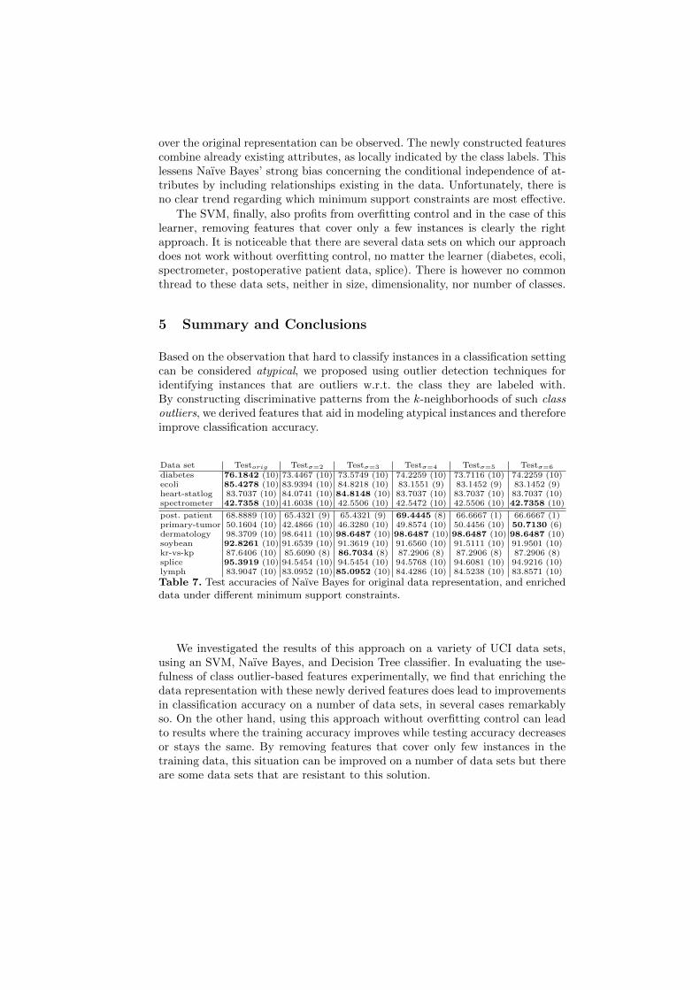
The SVM, finally, also profits from overfitting control and in the case of thislearner, removing features that cover only a few instances is clearly the rightapproach. It is noticeable that there are several data sets on which our approachdoes not work without overfitting control, no matter the learner (diabetes, ecoli,spectrometer, postoperative patient data, splice). There is however no commonthread to these data sets, neither in size, dimensionality, nor number of classes.

5 Summary and Conclusions

Based on the observation that hard to classify instances in a classification settingcan be considered atypical, we proposed using outlier detection techniques foridentifying instances that are outliers w.r.t. the class they are labeled with.By constructing discriminative patterns from the k-neighborhoods of such classoutliers, we derived features that aid in modeling atypical instances and thereforeimprove classification accuracy.

Data set Testorig Testσ=2 Testσ=3 Testσ=4 Testσ=5 Testσ=6

diabetes 76.1842 (10) 73.4467 (10) 73.5749 (10) 74.2259 (10) 73.7116 (10) 74.2259 (10)ecoli 85.4278 (10) 83.9394 (10) 84.8218 (10) 83.1551 (9) 83.1452 (9) 83.1452 (9)heart-statlog 83.7037 (10) 84.0741 (10) 84.8148 (10) 83.7037 (10) 83.7037 (10) 83.7037 (10)spectrometer 42.7358 (10) 41.6038 (10) 42.5506 (10) 42.5472 (10) 42.5506 (10) 42.7358 (10)

post. patient 68.8889 (10) 65.4321 (9) 65.4321 (9) 69.4445 (8) 66.6667 (1) 66.6667 (1)primary-tumor 50.1604 (10) 42.4866 (10) 46.3280 (10) 49.8574 (10) 50.4456 (10) 50.7130 (6)dermatology 98.3709 (10) 98.6411 (10) 98.6487 (10) 98.6487 (10) 98.6487 (10) 98.6487 (10)soybean 92.8261 (10) 91.6539 (10) 91.3619 (10) 91.6560 (10) 91.5111 (10) 91.9501 (10)kr-vs-kp 87.6406 (10) 85.6090 (8) 86.7034 (8) 87.2906 (8) 87.2906 (8) 87.2906 (8)splice 95.3919 (10) 94.5454 (10) 94.5454 (10) 94.5768 (10) 94.6081 (10) 94.9216 (10)lymph 83.9047 (10) 83.0952 (10) 85.0952 (10) 84.4286 (10) 84.5238 (10) 83.8571 (10)

Table 7. Test accuracies of Naıve Bayes for original data representation, and enricheddata under different minimum support constraints.

We investigated the results of this approach on a variety of UCI data sets,using an SVM, Naıve Bayes, and Decision Tree classifier. In evaluating the use-fulness of class outlier-based features experimentally, we find that enriching thedata representation with these newly derived features does lead to improvementsin classification accuracy on a number of data sets, in several cases remarkablyso. On the other hand, using this approach without overfitting control can leadto results where the training accuracy improves while testing accuracy decreasesor stays the same. By removing features that cover only few instances in thetraining data, this situation can be improved on a number of data sets but thereare some data sets that are resistant to this solution.

Our proposed approach is also not equally beneficial for all three classesof classifiers: the Naıve Bayes classifier profits most from the enriched repre-sentation, since the newly derived features overcome Naıve Bayes’ strong biasregarding conditional independence of attributes. The Decision Tree classifier,on the other hand, shows no improvement over the original representation on athird of the used data sets.

Generally, though, we have shown the merits of identifying class outliers andusing their neighborhoods to derive discriminative features to improve classifi-cation accuracy. We have limited us in this work to attribute-value data butthere is no reason why this approach cannot be extended, for instance, to graph-structured data, e.g. second-order representations of molecules.

References

1. Blake, C., Merz, C.: UCI repository of machine learning databases (1998), http://www.ics.uci.edu/~mlearn/MLRepository.html

2. Breunig, M.M., Kriegel, H.P., Ng, R.T., Sander, J.: Lof: Identifying density-basedlocal outliers. In: Chen, W., Naughton, J.F., Bernstein, P.A. (eds.) SIGMOD Con-ference. pp. 93–104. ACM (2000)

3. Cleveland, W., Devlin, S., E., G.: Regression by local fitting. Journal of Econo-metrics 37, 87–114 (1988)

4. Cohen, W.W.: Fast effective rule induction. In: Prieditis, A., Russell, S.J. (eds.)Proceedings of the Twelfth International Conference on Machine Learning. pp.115–123. Morgan Kaufmann, Tahoe City, California,USA (Jul 1995)

5. Cortes, C., Vapnik, V.: Support-vector networks. Machine Learning 20(3), 273–297(1995)

6. Cover, T., Hart, P.: Nearest neighbor pattern classification. Information Theory,IEEE Transactions on 13(1), 21 – 27 (Jan 1967)

7. Frank, E., Witten, I.H.: Data Mining: Practical Machine Learning Tools and Tech-niques with Java Implementations. Morgan Kaufmann (1999)

8. Lindgren, T., Bostrom, H.: Resolving rule conflicts with double induction. In:5th International Symposium on Intelligent Data Analysis. pp. 60–67. Springer,Berlin,Germany (Aug 2003)

9. Perez, E., Rendell, L.A.: Learning despite concept variation by finding structurein attribute-based data. In: ICML. pp. 391–399 (1996)

10. Quinlan, J.R.: C4.5: Programs for Machine Learning. Morgan Kaufmann (1993)11. Schapire, R.E.: The strength of weak learnability. Machine Learning 5, 197–227

(1990)12. Vilalta, R., Drissi, Y.: A characterization of difficult problems in classification. In:

Wani, M.A., Arabnia, H.R., Cios, K.J., Hafeez, K., Kendall, G. (eds.) ICMLA. pp.133–138. CSREA Press (2002)

13. Vilalta, R., Rish, I.: A decomposition of classes via clustering to explain and im-prove naive bayes. In: Lavrac, N., Gamberger, D., Todorovski, L., Blockeel, H.(eds.) ECML. LNCS, vol. 2837, pp. 444–455. Springer (2003)