Koukounari, A; Moustaki, I; Grassly, NC; Blake, IM; Basez...

Koukounari, A; Moustaki, I; Grassly, NC; Blake, IM; Basez, MG;Gambhir, M; Mabey, DC; Bailey, RL; Burton, MJ; Solomon, AW;Donnelly, CA (2013) Using a Nonparametric Multilevel Latent MarkovModel to Evaluate Diagnostics for Trachoma. American journal ofepidemiology. ISSN 0002-9262 DOI: 10.1093/aje/kws345

Downloaded from: http://researchonline.lshtm.ac.uk/989713/

DOI: 10.1093/aje/kws345

Usage Guidelines

Please refer to usage guidelines at http://researchonline.lshtm.ac.uk/policies.html or alterna-tively contact [email protected].

Available under license: http://creativecommons.org/licenses/by-nc-nd/2.5/

http://researchonline.lshtm.ac.uk/989713/

http://dx.doi.org/10.1093/aje/kws345

http://researchonline.lshtm.ac.uk/policies.html

mailto:[email protected]

1

WEB MATERIAL

Nonparametric multilevel LMM

LMM assumes that subjects (here children) are independent. However, in our study children are

nested within households and therefore the independence assumption is not fulfilled.

Multilevel LMMs account for the hierarchical structure of the data by allowing the latent health

states intercepts to vary across households. The random intercepts then allow for the probability

of belonging to a particular latent health state )( , tti jCP = to vary across households. Covariates

or contextual effects (household characteristics) can then be added as level-2 covariates to

explain the variation in those probabilities.

More specifically, in our study, the level-1 LMM is defined by four latent health states at each

time point and therefore a multinomial logistic regression model is used with J-1 random

intercepts at each time point where J is equal to the number of latent health states (here four or

three). One latent state is taken as a reference category (MPLUS uses the last latent health state

as the reference category) and therefore the introduction of the random intercepts allows the log-

odds of belonging to a specific latent health state at each time point to vary across households.

We follow here the nonparametric approach discussed by Henry and Muthen 2010 in which a

second latent class model is specified at level 2; in this model a new between-level (level-2)

categorical latent variable is denoted by Cb. A small number of level-2 latent classes capture the

level-2 variability in the distribution of the level-1 latent health state membership probabilities.

In this approach the normal distribution that is usually assumed for the random error of the

intercept is replaced with the assumption of a multinomial distribution. Through this approach,

clusters (i.e. households) are classified into a small number of types, rather than be placed on a

2

continuous scale (this would be the case if for instance household level random effects were

considered as drawn from a normal distribution). This yields a nonparametric multilevel LMM in

which there are not only latent categorical variables Ci with J latent health states of level-1 units

but also latent classes of level-2 units sharing the same parameter values (i.e. the random means;

that is the log-odds of membership in a particular level-1 latent health state).

The probability now that individual i in level-2 unit b is a member of latent health state j at time t

is a conditional probability and is given by:

(W.1)

where γjtm = γjt + utm , and γjt is the linear regression intercept for the log-odds of belonging to the

j latent health state rather than the last latent health state and utm is the household random effect

which comes from a discrete mixture distribution with m representing a specific mixture and

capturing the between households variation in the log-odds.

∑=

=== J

kktm

jtmbtbi mCbjCP

1

,,

)exp(

)exp()|(

γ

γ

3

Evaluation of the diagnostic accuracy of Polymerase Chain Reaction (PCR) ,

Trachomatous Inflammation-Follicular (TF), and Trachomatous Inflammation-Intense

(TI) for C. trachomatis infection (technical details for derivation of measures in Table 5)

In general, sensitivity (Sens) is the probability that an individual who is truly positive (denoted

TP) has a positive screening result (denoted +). Specificity (Spec) is the probability that an

individual who is truly negative (denoted TN) has a negative screening result (denoted -). The

positive predictive value (PPV) is the probability that an individual with a positive screening

result is truly positive. The negative predictive value (NPV) is the probability that an individual

with a negative screening result is truly negative.

Therefore,

Sens=)(

)(TPP

TPP ∩+

(W.2)

where )( TPP ∩+ is the joint probability of having a positive screening result and being truly

positive and )(TPP is the probability of a randomly chosen member of the study population

being screened to be truly positive.

Spec=)(

)(TNP

TNP ∩−

(W.3)

4

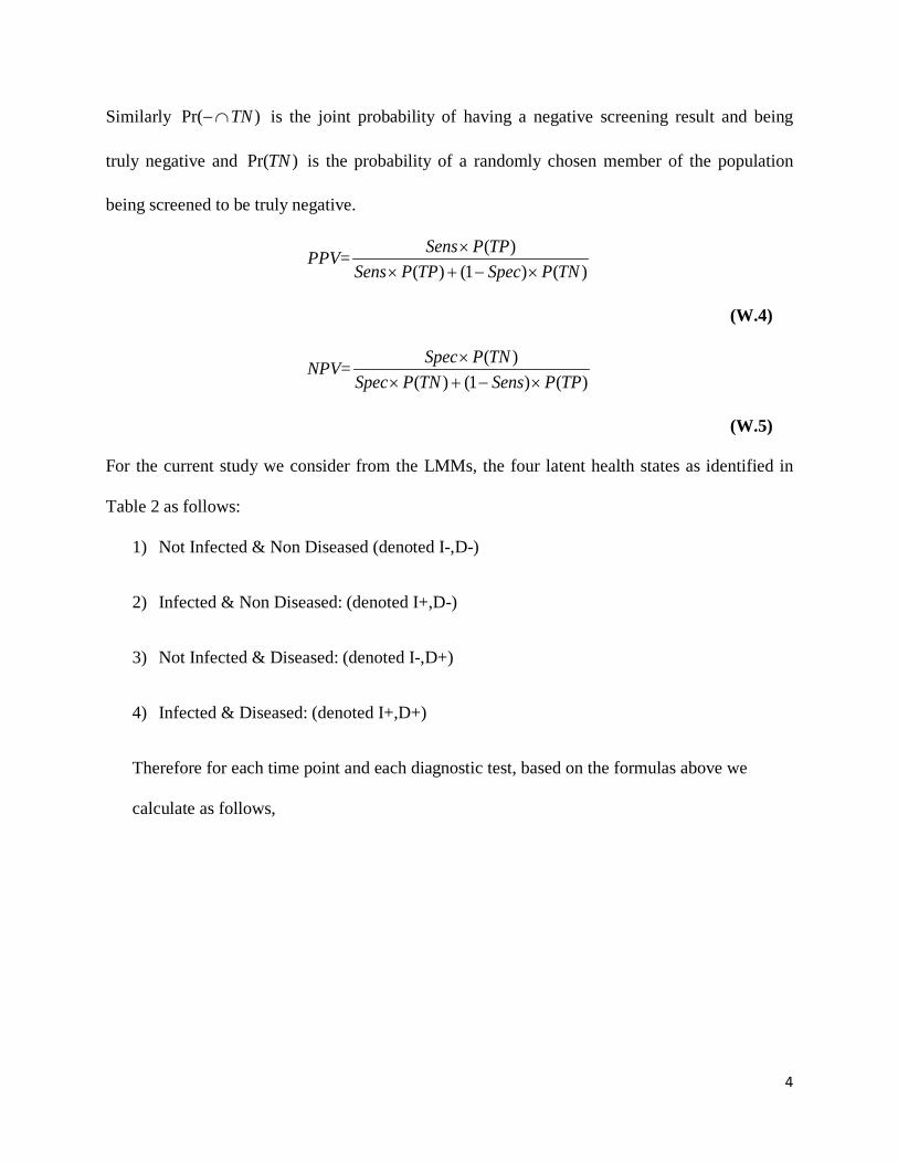
Similarly )Pr( TN∩− is the joint probability of having a negative screening result and being

truly negative and )Pr(TN is the probability of a randomly chosen member of the population

being screened to be truly negative.

PPV=)()1()(

)(TNPSpecTPPSens

TPPSens×−+×

×

(W.4)

NPV=)()1()(

)(TPPSensTNPSpec

TNPSpec×−+×

×

(W.5)

For the current study we consider from the LMMs, the four latent health states as identified in

Table 2 as follows:

1) Not Infected & Non Diseased (denoted I-,D-)

2) Infected & Non Diseased: (denoted I+,D-)

3) Not Infected & Diseased: (denoted I-,D+)

4) Infected & Diseased: (denoted I+,D+)

Therefore for each time point and each diagnostic test, based on the formulas above we

calculate as follows,

6

)D,I|( −++pP , )D,I|( +++pP , )D,I|( +−−pP , )D, I|( −−−pP , in (S.6-S.9) are conditional probabilities and represent the item response

probabilities ρ for the p diagnostic tests as estimated from the nonparametric multilevel LMMs contained in Table 2 in the main

article.

)D(I+,Pt − , )D(I+,Pt + , )D,(IPt +− , )D,(IPt −− in (W.6-W.9), are the prevalences η of the latent health states J. The subscript t denotes

that these quantities change at each time point of the studies as estimated from the nonparametric multilevel LMMs (these are

illustrated in Figure 4). After these calculations at each time point we take the average of each of these quantities.

Computation of approximated standard errors for the measures of Sensitivity (W.6), Specificity (W.7), PPV (W.8) and NPV

(W.9).

We employ here the Delta method for computing approximated standard errors for the functions of those parameters given in W.6-

W.9. For the prevalence estimates only we used the conservative standard errors from the fixed effects models since it was not feasible

to acquire those from the random effects models from the MPLUS output.

We provide below the first derivatives of the measures given in W.6-W.9 with respect to the individual parameters they are functions

of.

7

First derivatives of Sensitivity

w.r.t )D,I|( −++pP : 3,2,1,)]D(I+,P)D(I+,[P

)D(I+,P

tt

t1 =

++−−

= pS pt

w.r.t. )D,I|( +++pP : 3,2,1,)]D(I+,P)D(I+,[P

)D(I+,P

tt

t2 =

++−+

= pS pt

w.r.t. )D(I+,Pt − : 3,2,1;4,3,2,1,)]D(I+,P)D(I+,[P

)D(I+,P)]D,I|()D,I|([2

tt

t3 ==

++−

+×+++−−++= pt

PPS pp

pt

w.r.t. )D(I+,Pt + : 3,2,1;4,3,2,1,)]D(I+,P)D(I+,[P

)D(I+,P)]D,I|()D,I|([2

tt

t4 ==

++−

−×−++−+++= pt

PPS pp

pt

First derivatives of Specificity

w.r.t. )D, I|( −−−pP : 3,2,1,)]D,(IP)D,(I[P

)D,(IP

tt

t =−−++−

−−p

w.r.t. )D, I|( +−−pP : 3,2,1,)]D,(IP)D,(I[P

)D,(IP

tt

t =−−++−

+−p

w.r.t. )D, I( −−tP :

3,2,1;4,3,2,1,)]D,(IP)D,(I[P

)D,(IP)]D, I|()D,I|([2

tt

t ==−−++−

+−×−−−−+−−pt

PP pp

w.r.t. )D, I( +−tP :

3,2,1;4,3,2,1,)]D,(IP)D,(I[P

)D,(IP)]D, I|()D,I|([2

tt

t ==−−++−

−−×−−−−+−−pt

PP pp

10


)]D,(IP)D,I|()D,(IP)D,I|([)D,(IP(-1)2

tttt

ttt =−−×−−−++−×+−−+++×++−+−+×−+−

+−×+−−+−−×−−−×−+×p

PPPPPP

pppp

pp

w.r.t. )DI+,|( +−pP :


)]D,(IP)D,I|()D,(IP)D,I|([)D,(IP)1(2

tttt

ttt =−−×−−−++−×+−−+++×++−+−+×−+−

+−×+−−+−−×−−−×++×−p

PPPPPP

pppp

pp

w.r.t. )D,I|( −−−pP :


)]D,(IP)D,I|()D,(IP)D,I|([)D,(IP2

tttt

ttt =−−×−−−++−×+−−+++×++−+−+×−+−

++×++−+−+×−+−×−−p

PPPPPP

pppp

pp

w.r.t. )D,I|( +−−pP :


)]D,(IP)D,I|()D,(IP)D,I|([)D,(IP2

tttt

ttt =−−×−−−++−×+−−+++×++−+−+×−+−

++×++−+−+×−+−×+−p

PPPPPP

pppp

pp

w.r.t. )D,I( −+tP :


)]D,(IP)D,I|()D,(IP)D,I|([)D,I|()1(2

tttt

tt ==−−×−−−++−×+−−+++×++−+−+×−+−

+−×+−−+−−×−−−×−+−×−pt

PPPPPPP

pppp

ppp

w.r.t. )D,I( ++tP :

11


)]D,(IP)D,I|()D,(IP)D,I|([)D,I|()1(2

tttt

tt ==−−×−−−++−×+−−+++×++−+−+×−+−

+−×+−−+−−×−−−×++−×−pt

PPPPPPP

pppp

ppp

w.r.t. )D,I( −−tP :


)]D,(IP)D,I|()D,(IP)D,I|([)D,I|(2

tttt

tt ==−−×−−−++−×+−−+++×++−+−+×−+−

++×++−+−+×−+−×−−−pt

PPPPPPP

ppp

ppp

w.r.t. )D,I( +−tP :


)]D,(IP)D,I|()D,(IP)D,I|([)D,I|(2

tttt

tt ==−−×−−−++−×+−−+++×++−+−+×−+−

++×++−+−+×−+−×+−−pt

PPPPPPP

pppp

ppp

We provide below the steps for computing the standard errors for the Sensitivity measure for each item and time point. Let us define

with ),...,( 4,1 ptptpt SSS = the row vector for item p at time t with elements the first derivatives of the Sensitivity measure with respect

to the four parameters given in the row vector )]D,I(P),D,I(P),D,I|(P),D,I|([ ttp ++−++++−++= pPϑ .

According to the Delta method: Tptptpt SCovSySensitivitVar )()( ϑ=

where p = 1,2,3 and t= 1,2,3,4. Similarly we obtain variances and their corresponding standard errors for the rest of the constructed

measures (Specificity, PPV and NPV). We have calculated average values across time for all the measures (Sensitivity, Specificity,

12

PPV and NPV). Therefore the variance and standard errors of those averages are computed accordingly. In Table 4 in the main article

we provide 95 % confidence intervals using standard errors of those averages accordingly.

Latent Markov Models and Trachoma Diagnostics

13

WEB TABLE 1. Comparison of Alternative Latent Structures of the Single-Level LMMs Tanzania Children (N=367)

Item response probabilities are assumed to be constant over time Model J Transition

matrices r LL BIC AIC Sample

adjusted BIC 1 2 4 15 -1284.1 2656.8 2598.2 2609.2 2 2 2 11 -1290.3 2645.5 2602.6 2610.6 3 3 4 35 -1224.1 2654.9 2518.2 2543.8 4 3 2 23 -1242.6 2621.1 2531.3 2548.1 5 4 4 63 THE BEST LOG-

LIKELIHOOD VALUE WAS NOT

REPLICATEDa

NAb

NA NA

6 4 2 39 -1210.766 2651.8 2499.5 2528.1

Gambia Children (N= 587) Item response probabilities are assumed to be constant over time

Model J Transition matrices

r LL BIC AIC Sample adjusted BIC

1 2 4 15 -1267.3 2630.3 2564.7 2582.7 2 2 2 11 -1269.7 2609.6 2561.5 2574.7 3 3 4 35 -1235.1 2693.2 2540.0 2582.0 4 3 2 23 -1237.4 2621.4 2520.7 2548.3 5 4 4 63 THE BEST LOG-


REPLICATEDa

NAb

NA NA

6 4 2 39 -1207.552 2663.7 2493.1 2539.9

Abbreviations: r, number of free parameters; LL, corresponding maximum log-likelihood; BIC, Bayesian Information

Criterion; AIC, Akaike Information Criterion

Model 1, 3, 5: transition probabilities τ vary during all intervals; Model 2, 4, 6: baseline and follow-up τ vary such that

two transition probability matrices were fitted (one for 0-2 months and one common matrix for each subsequent

transition period).


14

Tanzania Children (N=367) Item response probabilities are allowed to vary over time

Model 1A, 3A, 5A: ρ and τ vary during all intervals; Model 2A, 4A, 6A: Baseline and follow-up τ vary such that two

transition probability matrices were fitted (one for 0-2 months and one common matrix for each subsequent transition

period).

aBecause of the multimodal likelihood of LMMs, and perhaps to the large r’s and power in the analyzed data, the best

log-likelihood value was not replicated. Consequently results of estimated parameters from this model cannot be

trusted

b Abbreviation NA, Not Available; as the best log-likelihood value was not replicated, results for BIC, AIC and

sample adjusted BIC form this model cannot be trusted either

Tables above report the LL, the number of latent health states k, parameters r, the BIC, AIC and

sample adjusted BIC value for the LMMs that were obtained during the model selection.



1A 2 4 39 -1220.9 2672.1 2519.7 2548.4 2A 2 2 17 -1253.4 2607.2 2540.8 2553.3 3A 3 4 71 -1179.1 2777.5 2500.2 2552.2 4A 3 2 32 -1219.4 2627.7 2502.7 2526.2 5A 4 4 111 THE BEST LOG-


REPLICATED

NA NA NA

6A 4 2 51 -1194.207 2689.6 2490.4 2527.8

Gambia Children (N= 587) Item response probabilities are allowed to vary over time



1A 2 4 39 -1238.5 2725.6 2555.0 2601.8 2A 2 2 17 -1256.1 2620.6 2546.2 2566.6 3A 3 4 71 -1194.9 2842.5 2531.9 2617.1 4A 3 2 32 -1221.2 2646.4 2506.4 2544.9 5A 4 4 111 THE BEST LOG-


REPLICATED

NA NA NA

6A 4 2 51 -1200.399 2725.9 2502.8 2564.2


15

Highlighted values in bold indicate the lowest obtained information criteria. The r is calculated by

Pη: number of latent health state prevalences; Pρ number of item response probabilities and Pτ

number of transition probabilities estimated.

The formula for the sample adjusted BIC value is nearly identical to the formula for BIC with the

difference that it replaces in the latter n with n* (where n* = (n + 2) / 24). Such information

criteria are not fully yet understood in statistical literature and how they particularly function for

LMMs. We explored a number of LMMs and determined as the most appropriate the model that

combined most of the following principles: reasonable goodness of fit, parsimony through

minimum values for most of the information criteria listed above as well as more apparent

biological plausibility of the phenomenon studied here.

We decided to keep the item response probabilities identical across times, because the meaning of

the latent health states also remains constant over time for these models. Although for Tanzania

BIC for Model 4, AIC for Model 6 and sample adjusted BIC for Model 6 were the smallest. The

item response probabilities for Model 6 did not yield latent health states that were biologically

interpretable. Thus, we selected Model 4 for further testing.

For The Gambia, BIC was the smallest for Model 2; however AIC and sample adjusted BIC were

the smallest for Model 6. Because Model 6 yielded biologically interpretable latent health states,

we selected Model 6 for further testing.


16

WEB TABLE 2. Fit Criteria for Nonparametric Multilevel Latent Markov Model (LMM) Specification

Tanzania Children (N=367)

Model r m LL

BIC AIC Sample adjusted

BIC

p-value*

7 22 -1097.3 2330.4 2240.6 2257.4 8 40 2 -1043.0 2322.1 2185.2 2208.6 <0.001

Remarks: When nonparametric multilevel models were fitted to the 5 timepoints under study for both Tanzania and

Gambia, warning messages were obtained about the standard errors of some of the model parameters that they may

not be trustworthy most probably as an indication of model nonidentification. Therefore, all models presented in the

above table were also restricted to the first 4 timepoints of the studies: baseline, 2, 6 and 12 months. Highlighted

values in bold indicate the lowest obtained information criteria.

Abbreviations: r, number of free parameters; m, number of between-level latent classes at the random coefficients

part; LL, corresponding maximum log-likelihood; BIC, Bayesian Information Criterion; AIC, Akaike Information

Criterion .

Model 7: Fixed effects LMM with 3 and 4 latent health states for Tanzania and Gambia, respectively; There were two

transition probability matrices in each case. Model 8: Nonparametric multilevel LMM model with 3 and 4 latent health

states for Tanzania and Gambia, respectively and 2 between-level latent classes for both countries; *p-value compares

the LL between Models 7 and 8; because for both datasets these are significant, the results all imply that Model 8

provides significantly improved fit over Model 7.

Web Table 1 reports the LL value, the number of parameters r and the information criteria for

single-level and nonparametric multilevel LMM models. All results reported in main text are

estimated from Model 8. Model 7 for Tanzania is the same structure as model 4 in Web Table 2,

Gambia Children (N=587)

Model r m LL

BIC AIC Sample adjusted

BIC

p-value*

7 38 -1071.4 2391.5 2220.9 2267.7 8 52 2 -976.6 2284.8 2057.3 2119.7 <0.001


17

except fitted to only data from 4 timepoints and of course for Gambia is the same structure as

model 6 in Web Table 2 except fitted to only data from 4 time points. The r is calculated as in

single-level models by Pη: number of latent health state prevalences; Pρ number of item response

probabilities and Pτ number of transition probabilities estimated. In technical terms of MPLUS and

the nonparametric multilevel models fitted here, latent categorical variables Ci,t that represent the

level-1 health states at each time point t were regressed on the new categorical latent variable Cb

and thus the parameters estimated from these regressions are the additional parameters now

contained in Web Table 1 if compared with fixed effects models in Web Table 2.

Koukounari, A; Moustaki, I; Grassly, NC; Blake, IM; Basez...

Documents

Transcript of Koukounari, A; Moustaki, I; Grassly, NC; Blake, IM; Basez...