1

The Pioneer Anomaly

An Investigation by

A Radio Amateur

Knut K. A. Najmann, DJ1ZN

“Out There”

In Gaertringen, Germany

2

The Pioneer Anomaly

An Investigation by Knut K. A. Najmann April 27, 2011

Introduction

It was mid 2008 when I first heard about the famous “Pioneer Anomaly”. The detailed information about

this famous “Pioneer Anomaly” I got was from PD Dr. Roland Speith in his “Antrittsvorlesung in

Tuebingen” June 4 2008, which my friend Klaus Mischke attended and who informed me about this

interesting mystery. Since 1998, when the Pioneer Anomaly was reported by J.D. Anderson [1] for the

first time (it was discovered 18 years earlier), many articles have been written on this phenomena. I

studied the various descriptions which I found in the internet. All kinds of explanations have been

published and tried to explain the small but measurable acceleration backwards to our Sun. The

measured unexplained acceleration yields a deviation of the distance of the probes to our sun of about

100000 km within 15 years. This means, according to the measurements the Pioneer probes are further

away than they actually are. This deviation has been calculated for both, Pioneer 10 and Pioneer 11.

The NASA experts have tried hard to explain the reason for this famous “Pioneer Anomaly” as it has been

named. In several articles it was mentioned, that “hopefully some one out there” will be able to give a

good explanation. “New Physics” are allowed if the calculations yield the deviation as predicted.

I am one of the interested people “out there” who assumes he has found an explanation of the Pioneer

Anomaly. Using the data as published by the NASA and my calculations, the Pioneer probes are where

they should be.

My calculation are based on, not “new physics” but as I name it, correct physics. In order to proof the

correctness of my calculations, I propose an experiment which, if performed, will show the correctness

of my assumptions or vise versa. The proposed experiment has not been performed before.

During my investigation I also thought, the Voyager probes data may give some insight to the Pioneer

Anomaly. I therefore studied the data for both Voyager 1 and Voyager 2. The detailed data for these

investigations I found in the internet. During the careful investigation I discovered something in the data

which to me is very strange. It is the velocity of the probes relative to our earth. I calculated in detail the

velocity myself and came to the conclusion: there is something wrong with the measurement data or in

the calculated results as published by NASA.

I describe the investigation in detail in a separate document which I named “The Voyager Mystery”.

3

The two chapters of this document dealing with the Pioneer Anomaly are:

1. The Pioneer Anomaly – an explanation

This chapter describes how the distance of a space probe is calculated using an

electromagnetic pulse send from Earth to the probe and resend back to earth, measuring the

elapsed time, the so called Round Trip Light Time, “RTLT”. The evaluation of a new formula is

derived.

2. The IME-Experiment

In this chapter I describe an experiment which should proof or disproof my way to calculate the

distance of a space probe using electromagnetic pulses from two different sources and

measuring the elapsed Round Trip Pulse Time, “RTPT”. IME stands for ISS-Mars-Earth.

The Pioneer Anomaly – an explanation

Before I started the detailed investigation in order to understand what the famous anomaly is and if I

could understand it, I looked for available data describing the behavior of space probes in space. I did not

think that the analysis oft the Voyager 2 data would be such a time consuming task. But it became a very

interesting one. I now understand somewhat better what happens to the various space probes out there

in our solar system and away from it. Especially I was very happy that my calculations showed accurately

how Voyager 2 speeds out from the solar system. All the calculations have been performed without

using special programs. An old TI 59 pocket PC and mainly Microsoft Excel running on a 1GHz PC was

used for all the various calculations. With all the details in mind I thought I would be ready to look in

more detail at the famous Pioneer Anomaly.

I studied quite a few of the many reports and descriptions on the subject which are accessible from the

internet. J.D. Anderson and his colleges wrote the first and very detailed report about their famous

problem. I do not understand all of the interesting details but I tried to understand the basics, how the

famous problem has been discovered. I will include in this document the two short paragraphs which I

thought would help to understand and maybe help to solve this very interesting problem.

After the careful analysis of the Voyager 2 data and the detailed insights I got, I am confident that I will

be able to describe a solution for the problem. To mention it here already, it is completely different

from all the interesting proposals which have been published so far.

4

Attacking the Pioneer Anomaly Problem:

Description of the basic measurements:

There are 3 types of measurements which determine the exact position and the velocity of a space probe

in space. These measurements are all performed by 3 DSN stations distributed on Earth. The 3 types of

measurements are (se also a link at [2]):

1. Direction – where is a space probe? In which direction do we have to aim the antennas?

2. Distance – how far away is it?

3. Velocity – how fast is it moving away from us?

The only two measurements and their results which are the cause for the Pioneer Anomaly are the

measurement of the distance and the measurement of the velocity.

My understanding how these measurements are used is the following:

Distance is determined by measurement of the round trip light time RTLT.

Velocity is determined by measurement of frequency differences due to Doppler shift between

transmitted signal frequency from Earth and received signal frequency on Earth. The signal is

retransmitted from the space probe after changing the outgoing frequency by a fixed multiplier.

The determined distance is always with respect to Earth. Using the well known astronomical parameters,

the distance relative to our Sun can then be calculated.

Two distance measurements at two different times can be used to determine the velocity too – at least

the average velocity – at these times.

The velocity determined can be used to predict the distance from one position to a new position after a

given time.

Both types of measurements therefore should give identical results for distance as well as velocity.

Definition of distance: The distance as I understand it is a result from the RTLT calculation i.e. the

distance between the position of the DSN station when the signal was sent from Earth up to the space

probe and the position where the space probe was, when the signal has reached the space probe.

Definition of velocity: Using the Two Way Doppler Shift Formula, the calculated velocity is the relative

velocity between the space probe and the Earth.

With all of the above data the distance as well as the velocity relative to any other position, for example

relative to the Sun can be calculated.

5

John Anderson discovered – as I understand it – that the distance as calculated by very accurate velocity

measurements always is shorter than the distance calculated by the model using RTLT measurements.

These velocity measurements are so precise, that for example the slow velocity of the Earth turning

around itself can be plotted in diagrams. I found a diagram in the report about the Pioneer Anomaly

which I copied and which is shown in Fig.1. Since the actual values are not given, I added numbers

manually which I think are reasonable values. The diagram shows the fantastic cooperation between the

three DSN stations. The signal sent up by DSN-1 may have to be picked up by DSN-2 because the RTLT is

so extreme long.

Possible reasons for the cause of the Pioneer Anomaly:

This little truth Table P-1 describes the possible combinations which I investigated to get a clear

understanding of the problem.

Table P1:

E1 E2 Result

C C A

C W B

W C C

W W D

Explanation:

E1: The Two Way Doppler Shift Formula used to calculate the relative velocity of a space craft relative to

Earth.

E2: The formula to calculate the distance of a spacecraft from the position of a DSN station on earth.

C: Means correct

W: Means wrong

A to D: Results of combinations

Result A:

Here we assume that both equations are correct and the results of the calculation show differences

between each other. According to the report about the Pioneer Anomaly the calculated velocity if used

to calculate the distance results in somewhat lower values. After a spacecraft has reached a distance far

away from Sun as well as Earth, it´s velocity has settled down and is pretty much constant. The Sun will

6

forever pull on it, but it´s influence is becoming negligible. Since the velocity stays pretty much constant

with time, the failure which was found stays constant too. Because the two equations can´t be blamed

in this combination, John Anderson and his colleges decided to use an unknown acceleration towards the

sun as a reason for the discrepancy. The distance calculated by using the RTLT formula was found to be

always somewhat larger than by calculations using 2 velocity measurements. Fig.2 is a copy of a short

paragraph of the document. It shows, how they thought about the problem. A constant decrease of

velocity with time can pretty well be described as a constant acceleration towards the Sun. I think it was

a good idea. Now everybody could start thinking about what is causing this strange acceleration. Many

interesting reports have been written in the meantime and describe nice solutions. Up to now none of

the proposals has been accepted as a solution to the famous anomaly problem.

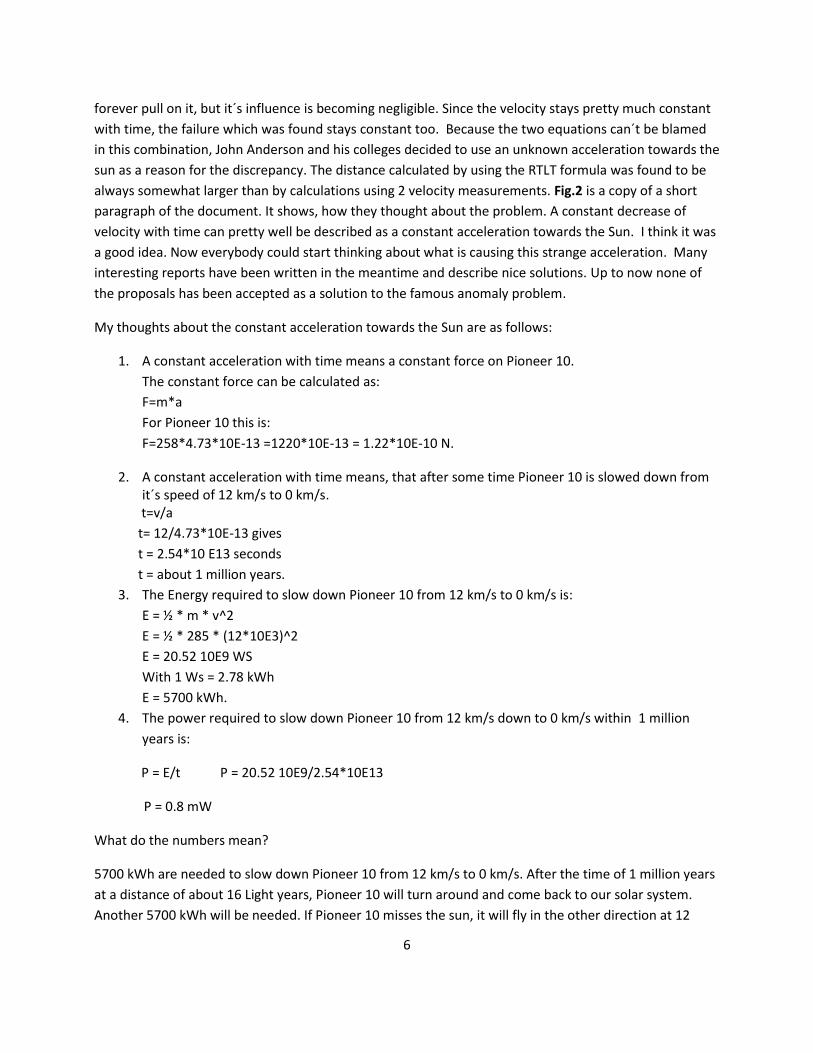
My thoughts about the constant acceleration towards the Sun are as follows:

1. A constant acceleration with time means a constant force on Pioneer 10.

The constant force can be calculated as:

F=m*a

For Pioneer 10 this is:

F=258*4.73*10E-13 =1220*10E-13 = 1.22*10E-10 N.

2. A constant acceleration with time means, that after some time Pioneer 10 is slowed down from it´s speed of 12 km/s to 0 km/s.

t=v/a

t= 12/4.73*10E-13 gives

t = 2.54*10 E13 seconds

t = about 1 million years.

3. The Energy required to slow down Pioneer 10 from 12 km/s to 0 km/s is:

E = ½ * m * v^2

E = ½ * 285 * (12*10E3)^2

E = 20.52 10E9 WS

With 1 Ws = 2.78 kWh

E = 5700 kWh.

4. The power required to slow down Pioneer 10 from 12 km/s down to 0 km/s within 1 million

years is:

P = E/t P = 20.52 10E9/2.54*10E13

P = 0.8 mW

What do the numbers mean?

5700 kWh are needed to slow down Pioneer 10 from 12 km/s to 0 km/s. After the time of 1 million years

at a distance of about 16 Light years, Pioneer 10 will turn around and come back to our solar system.

Another 5700 kWh will be needed. If Pioneer 10 misses the sun, it will fly in the other direction at 12

7

km/s until it will again return. And so on. It would be the first artificial comet, a nice one with two

apogees.

I have my doubts that this will ever happen, regardless whether the energy is delivered by Pioneer itself

or by the Sun or any other black magic force.

Summary for result of combination A:

My opinion: Result of combination A is not possible.

Result B:

This is the next combination. Equation 1 – the Two Way Doppler Shift Formula - is assumed to be correct

and there is something wrong with equation 2. What could it be? If there is something wrong the results

from the correct equation must differ only very slightly from the basic equation to calculate a distance,

based on RTLT measurements.

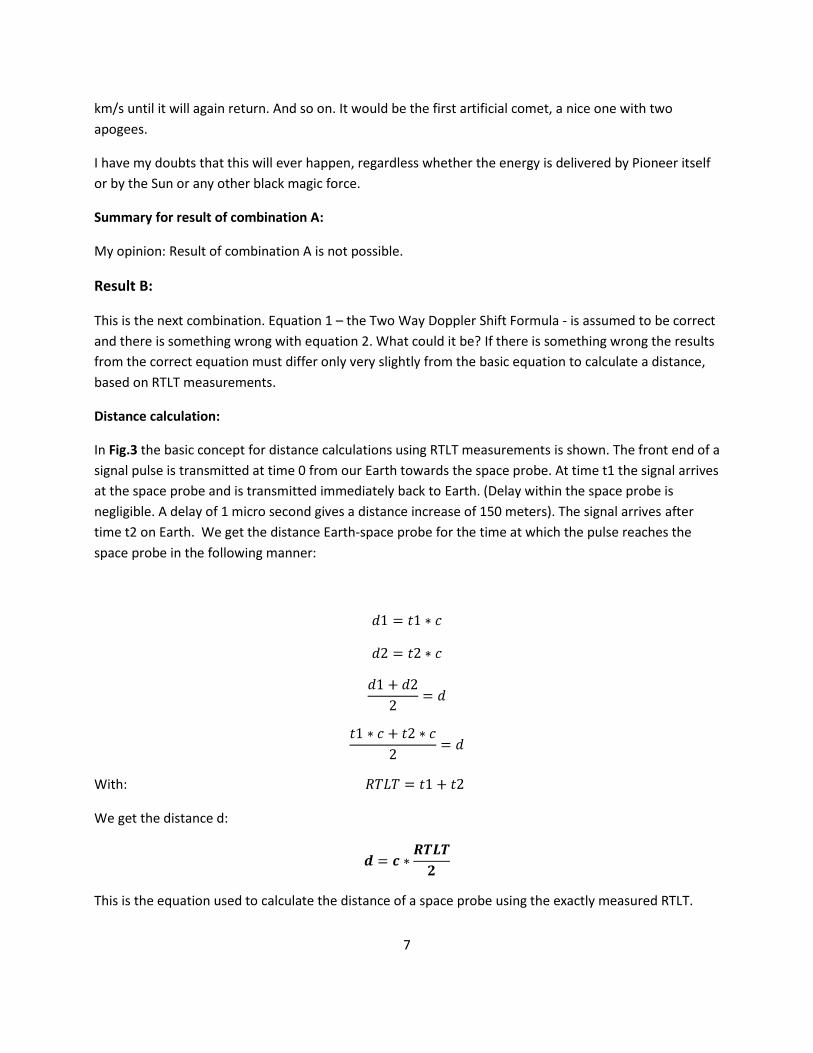
Distance calculation:

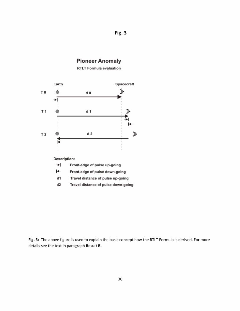
In Fig.3 the basic concept for distance calculations using RTLT measurements is shown. The front end of a

signal pulse is transmitted at time 0 from our Earth towards the space probe. At time t1 the signal arrives

at the space probe and is transmitted immediately back to Earth. (Delay within the space probe is

negligible. A delay of 1 micro second gives a distance increase of 150 meters). The signal arrives after

time t2 on Earth. We get the distance Earth-space probe for the time at which the pulse reaches the

space probe in the following manner:

With:

We get the distance d:

This is the equation used to calculate the distance of a space probe using the exactly measured RTLT.

8

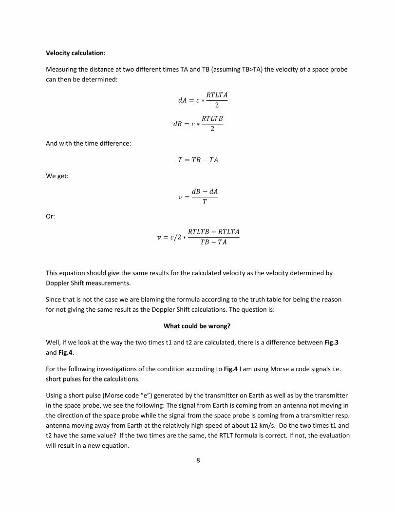
Velocity calculation:

Measuring the distance at two different times TA and TB (assuming TB>TA) the velocity of a space probe

can then be determined:

And with the time difference:

We get:

Or:

This equation should give the same results for the calculated velocity as the velocity determined by

Doppler Shift measurements.

Since that is not the case we are blaming the formula according to the truth table for being the reason

for not giving the same result as the Doppler Shift calculations. The question is:

What could be wrong?

Well, if we look at the way the two times t1 and t2 are calculated, there is a difference between Fig.3

and Fig.4.

For the following investigations of the condition according to Fig.4 I am using Morse a code signals i.e.

short pulses for the calculations.

Using a short pulse (Morse code “e”) generated by the transmitter on Earth as well as by the transmitter

in the space probe, we see the following: The signal from Earth is coming from an antenna not moving in

the direction of the space probe while the signal from the space probe is coming from a transmitter resp.

antenna moving away from Earth at the relatively high speed of about 12 km/s. Do the two times t1 and

t2 have the same value? If the two times are the same, the RTLT formula is correct. If not, the evaluation

will result in a new equation.

9

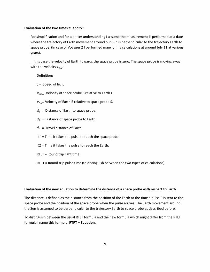
Evaluation of the two times t1 and t2:

For simplification and for a better understanding I assume the measurement is performed at a date

where the trajectory of Earth movement around our Sun is perpendicular to the trajectory Earth to

space probe. (In case of Voyager 2 I performed many of my calculations at around July 11 at various

years).

In this case the velocity of Earth towards the space probe is zero. The space probe is moving away

with the velocity

Definitions:

c = Speed of light

Velocity of space probe S relative to Earth E.

Velocity of Earth E relative to space probe S.

Distance of Earth to space probe.

Distance of space probe to Earth.

Travel distance of Earth.

= Time it takes the pulse to reach the space probe.

= Time it takes the pulse to reach the Earth.

RTLT = Round trip light time

RTPT = Round trip pulse time (to distinguish between the two types of calculations).

Evaluation of the new equation to determine the distance of a space probe with respect to Earth

The distance is defined as the distance from the position of the Earth at the time a pulse P is sent to the

space probe and the position of the space probe when the pulse arrives. The Earth movement around

the Sun is assumed to be perpendicular to the trajectory Earth to space probe as described before.

To distinguish between the usual RTLT formula and the new formula which might differ from the RTLT

formula I name this formula: RTPT – Equation.

10

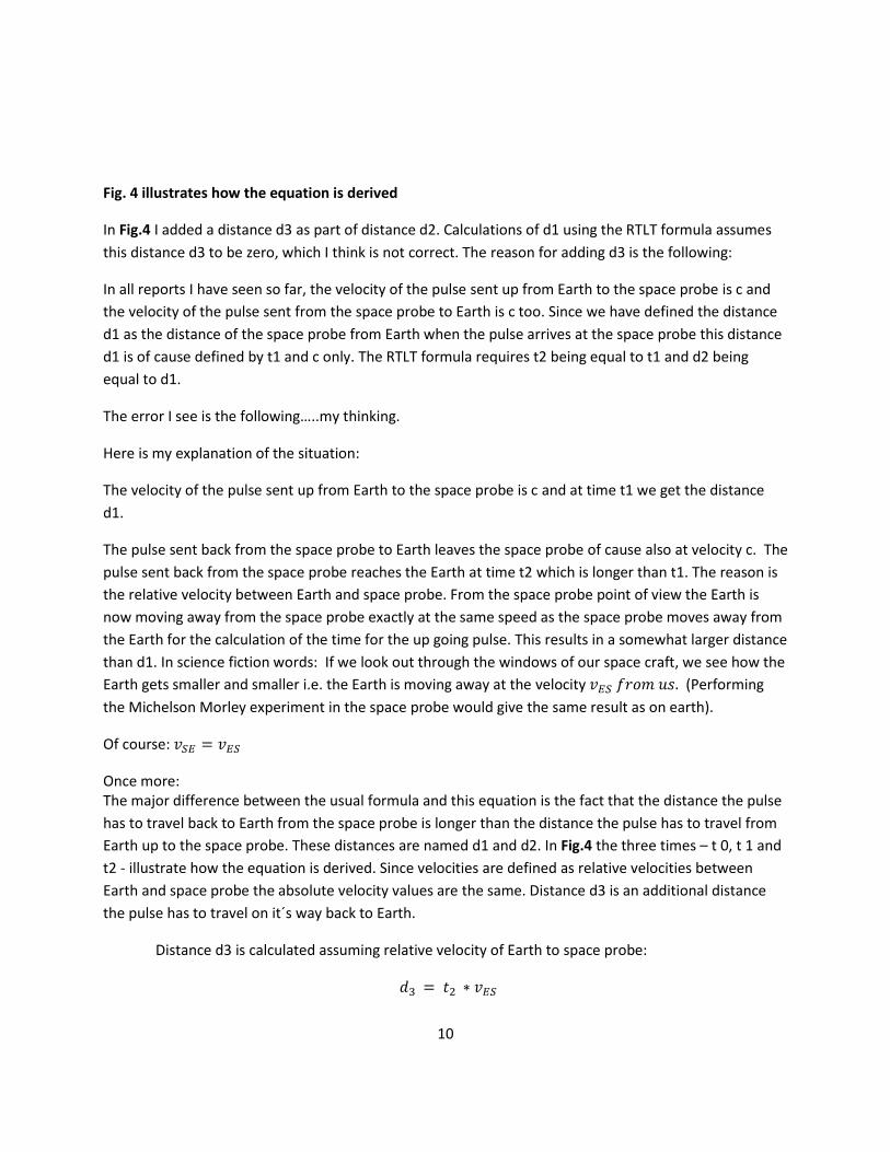
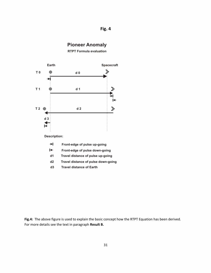
Fig. 4 illustrates how the equation is derived

In Fig.4 I added a distance d3 as part of distance d2. Calculations of d1 using the RTLT formula assumes

this distance d3 to be zero, which I think is not correct. The reason for adding d3 is the following:

In all reports I have seen so far, the velocity of the pulse sent up from Earth to the space probe is c and

the velocity of the pulse sent from the space probe to Earth is c too. Since we have defined the distance

d1 as the distance of the space probe from Earth when the pulse arrives at the space probe this distance

d1 is of cause defined by t1 and c only. The RTLT formula requires t2 being equal to t1 and d2 being

equal to d1.

The error I see is the following…..my thinking.

Here is my explanation of the situation:

The velocity of the pulse sent up from Earth to the space probe is c and at time t1 we get the distance

d1.

The pulse sent back from the space probe to Earth leaves the space probe of cause also at velocity c. The

pulse sent back from the space probe reaches the Earth at time t2 which is longer than t1. The reason is

the relative velocity between Earth and space probe. From the space probe point of view the Earth is

now moving away from the space probe exactly at the same speed as the space probe moves away from

the Earth for the calculation of the time for the up going pulse. This results in a somewhat larger distance

than d1. In science fiction words: If we look out through the windows of our space craft, we see how the

Earth gets smaller and smaller i.e. the Earth is moving away at the velocity (Performing

the Michelson Morley experiment in the space probe would give the same result as on earth).

Of course:

Once more: The major difference between the usual formula and this equation is the fact that the distance the pulse

has to travel back to Earth from the space probe is longer than the distance the pulse has to travel from

Earth up to the space probe. These distances are named d1 and d2. In Fig.4 the three times – t 0, t 1 and

t2 - illustrate how the equation is derived. Since velocities are defined as relative velocities between

Earth and space probe the absolute velocity values are the same. Distance d3 is an additional distance

the pulse has to travel on it´s way back to Earth.

Distance d3 is calculated assuming relative velocity of Earth to space probe:

11

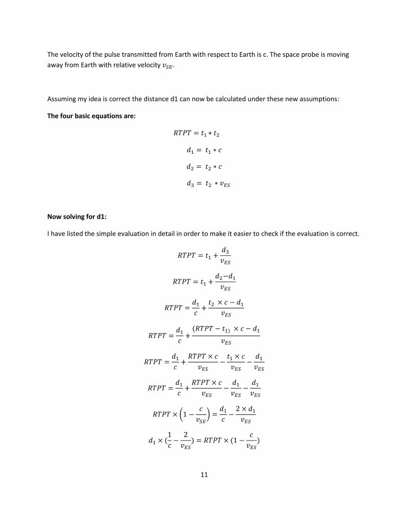
The velocity of the pulse transmitted from Earth with respect to Earth is c. The space probe is moving

away from Earth with relative velocity

Assuming my idea is correct the distance d1 can now be calculated under these new assumptions:

The four basic equations are:

+

Now solving for d1:

I have listed the simple evaluation in detail in order to make it easier to check if the evaluation is correct.

12

===========================================

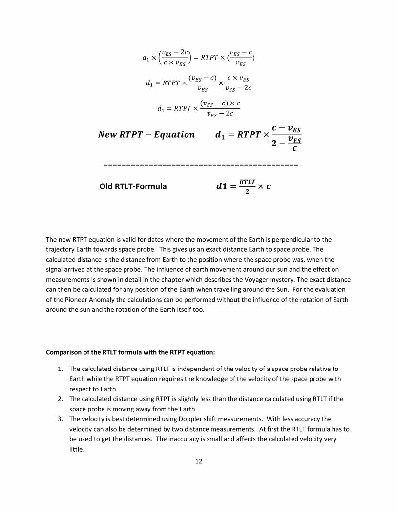
Old RTLT-Formula

The new RTPT equation is valid for dates where the movement of the Earth is perpendicular to the

trajectory Earth towards space probe. This gives us an exact distance Earth to space probe. The

calculated distance is the distance from Earth to the position where the space probe was, when the

signal arrived at the space probe. The influence of earth movement around our sun and the effect on

measurements is shown in detail in the chapter which describes the Voyager mystery. The exact distance

can then be calculated for any position of the Earth when travelling around the Sun. For the evaluation

of the Pioneer Anomaly the calculations can be performed without the influence of the rotation of Earth

around the sun and the rotation of the Earth itself too.

Comparison of the RTLT formula with the RTPT equation:

1. The calculated distance using RTLT is independent of the velocity of a space probe relative to

Earth while the RTPT equation requires the knowledge of the velocity of the space probe with

respect to Earth.

2. The calculated distance using RTPT is slightly less than the distance calculated using RTLT if the

space probe is moving away from the Earth

3. The velocity is best determined using Doppler shift measurements. With less accuracy the

velocity can also be determined by two distance measurements. At first the RTLT formula has to

be used to get the distances. The inaccuracy is small and affects the calculated velocity very

little.

13

Checking the RTPT equation:

1. A simple check is to set the velocity of the space probe to zero. This must result in the RTLT

formula - which it does.

If the equation is correct, a good check will be to calculate the distance Pioneer 10 travels within 15

years using the RTLT formula and compare it with the distance Pioneer 10 travels calculated according to

the RTPT equation. Subtracting the second distance from the first one should result in a distance which

is equal or at least close to the distance Pioneer 10 is pulled back by the anomaly acceleration during

that time. In several of the reports describing the Pioneer anomaly this distance was estimated to about

100000km [5], [6]. In one report [4] I found 1 million km as the difference distance. I assumed this to be

a typing error. This report gives also a good explanation about the Pioneer Anomaly (in German).

http://www.safog.com/home/pioneer_anomalie

2. Calculation of travel distance for two time spans of 15 years each:

Reason for choosing two different time spans: Check if there is a noticeable difference between

different time spans.

Assumptions:

1. Space probe is Pioneer 10

2. Calculation performed for two time spans (two just for comparison) of 15 years each.

3. Start year is 1985

4. End year is 2005

5. Data extracted from: Helio Web Browser Results, Pioneer 10 position listing. [2]

http://omniweb.gsfc.nasa.gov/egi/models/helios.cgi

6. Raw data similar to Voyager data from the Voyager Status Reports is not available.

Available Data for each day: AU (Distance of Pioneer 10 from Earth) and Ecliptic latitude angle.

Only the AU values have been used for the investigation, since the Ecliptic latitude angle is

around 3 degrees only. For the comparison of the two equations it has a negligible effect. The

AU values are accurate to 0.01 AU. For the comparison of the results from the two equations -

RTLT, RTPT -the accuracy has no effect.

14

Distance calculation for 15 years of time span:

Tables P-2 to P-5 show, how the travel distance for two time spans of 15 years was calculated. First

using the RTPT equation and second using the anomaly acceleration values. The results are then

compared, also with the value which I found in the literature.

Table P-2:

This table is like an Excel type table and is used to calculate for several years on January first the

distance in km of Pioneer 10 to Earth. The average velocity within one year before and after years

1985, 1990, 1995, 2000and 2005 was used to calculate the velocity of Pioneer 10 on January first

for 5 years between 1985 and 2005. The way how the table was filled with the data is described

below the table.

Data used:

1 AU = 149 597 870 km

c = 299 792, 458 km/s

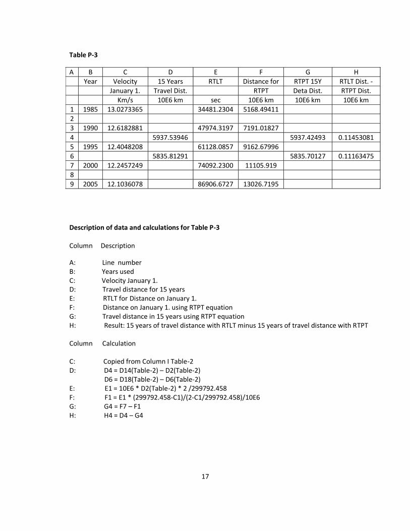
Table P-3:

The purpose of this table was to calculate the distance Pioneer 10 has travelled within the two

time spans of 15 years. The two time spans are 1985 to 2000 and 1990 to 2005. For example: from

1985 to 2000 Pioneer 10 has travelled 5937.53946*10E6 km (Cell D4).

The RTLT was also used to calculate the velocity for each of the fife years. These values are

necessary to calculate RTPT. Now the actual distance using the RTPT equation was determined.

For example, the RTPT distance on January 1. 1985 is 5168.49411*10E6 km (Cell F1) compared to

5168.60641*10E6 km (Cell D2 in Table P-2) as calculated from the AU values.

The travel distance within 15 years can now be calculated for the distances based on the AU values

and the distances calculated using the RTPT equation.

For example, in cell D4 the travel distance from January 1. 1985 to January 1. 2000 is

5937.53946*10E6 km based on the AU data, while in cell G4 the RTPT value is 5937.42493*10E6

km. The difference between the two should correspond to the distance Pioneer 10 is pulled back

due to the anomaly effect.

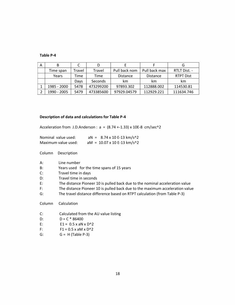
Table P-4

Purpose of this table is to show how the “pull-back” distance due to the Pioneer Anomaly

acceleration for the two time spans is calculated:

The two values used - nom and max - for the anomaly acceleration are from the Pioneer Anomaly

report.

Nominal value labeled: aN

Maximum value labeled: aM

15

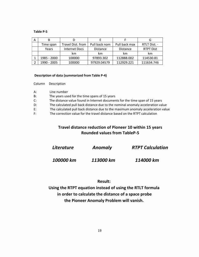
Table P-5:

This table summarizes the data from Table P-4.

At the bottom of the table the values for the pull back distance are compared with the result of the

RTPT calculation.

The difference between the value due to the anomaly acceleration and the value based on the

RTPT calculation is about 1 percent. Nice!?

The result of the investigation is given also on the bottom of Table P-5.

16

Table P-2

A B C D E F G H I

Year AU Distance Days Seconds Travel Average January 1.

10E6 Per Per Year Distance Velocity Velocity

km Year sec 10E6 km Km/s Km/s

1 1984 31.79 4755.71629 366 31622400 412.890121 13.05688756

2 1985 34.55 5168.60641 365 31536000 409.898164 12.99778551 13.0273365

3 1986 37.29 5578.50457

4

5 1989 45.40 6791.7433 365 31536000 399.426313 12.66572529

6 1990 48.07 7191.16961 365 31536000 396.434356 12.57085095 12.6182881

7 1991 50.72 7587.60397

8

9 1994 58.63 8770.92312 365 31536000 391.946419 12.42853943

10 1995 61.25 9162.86954 365 31536000 390.450441 12.38110225 12.4048208

11 1996 63.86 9553.31998

12

13 1999 71.66 10720.1834 365 31536000 385.962505 12.23879073

14 2000 74.24 11106.1459 366 31622400 387.458483 12.25265898 12.2457249

15 2001 76.83 11493.6044

16

17 2004 84.52 12644.012 366 31622400 382.970547 12.11073629

18 2005 87.08 13026.9825 365 31536000 381.474596 12.09647921 12.1036078

19 2006 89.63 13408.4571

Description of data and calculations for Table P-2 Column Description/Calculation A: Line number B: Years used C: Distance in AU at January 1. http://cohoweb.gsfc.nasa.gov/helios D: Distance in 10E6 km for January 1. E: Number of days for year F: Seconds for year G: Travel distance for one year H: Average velocity within one year I: Velocity January 1. D: Distance in 10E6 km D=149.59787*C F: F = E * 86400 G: G1 = D2 – D1 H: H1 = 10E6 + G1/F1 I: I2 = (H1+H2)/2

17

Table P-3

A B C D E F G H

Year Velocity 15 Years RTLT Distance for RTPT 15Y RTLT Dist. -

January 1. Travel Dist. RTPT Deta Dist. RTPT Dist.

Km/s 10E6 km sec 10E6 km 10E6 km 10E6 km

1 1985 13.0273365 34481.2304 5168.49411

2

3 1990 12.6182881 47974.3197 7191.01827

4 5937.53946 5937.42493 0.11453081

5 1995 12.4048208 61128.0857 9162.67996

6 5835.81291 5835.70127 0.11163475

7 2000 12.2457249 74092.2300 11105.919

8

9 2005 12.1036078 86906.6727 13026.7195

Description of data and calculations for Table P-3 Column Description

A: Line number B: Years used C: Velocity January 1. D: Travel distance for 15 years E: RTLT for Distance on January 1. F: Distance on January 1. using RTPT equation G: Travel distance in 15 years using RTPT equation H: Result: 15 years of travel distance with RTLT minus 15 years of travel distance with RTPT Column Calculation C: Copied from Column I Table-2 D: D4 = D14(Table-2) – D2(Table-2) D6 = D18(Table-2) – D6(Table-2) E: E1 = 10E6 * D2(Table-2) * 2 /299792.458 F: F1 = E1 * (299792.458-C1)/(2-C1/299792.458)/10E6 G: G4 = F7 – F1 H: H4 = D4 – G4

18

Table P-4

A B C D E F G

Time span Travel Travel Pull back nom Pull back max RTLT Dist. -

Years Time Time Distance Distance RTPT Dist

Days Seconds km km km

1 1985 - 2000 5478 473299200 97893.302 112888.002 114530.81

2 1990 - 2005 5479 473385600 97929.04579 112929.221 111634.746

Description of data and calculations for Table P-4 Acceleration from J.D.Anderson : a = (8.74 +-1.33) x 10E-8 cm/sec^2 Nominal value used: aN = 8.74 x 10 E-13 km/s^2 Maximum value used: aM = 10.07 x 10 E-13 km/s^2 Column Description

A: Line number B: Years used for the time spans of 15 years C: Travel time in days D: Travel time in seconds E: The distance Pioneer 10 is pulled back due to the nominal acceleration value F: The distance Pioneer 10 is pulled back due to the maximum acceleration value G: The travel distance difference based on RTPT calculation (from Table P-3)

Column Calculation C: Calculated from the AU value listing D: D = C * 86400 E: E1 = 0.5 x aN x D^2 F: F1 = 0.5 x aM x D^2 G: G = H (Table P-3)

19

Table P-5

A B D E F G

Time span Travel Dist. from Pull back nom Pull back max RTLT Dist. -

Years Internet Docs Distance Distance RTPT Dist

km km km km

1 1985 - 2000 100000 97893.302 112888.002 114530.81

2 1990 - 2005 100000 97929.04579 112929.221 111634.746

Description of data (summarized from Table P-4)

Column Description

A: Line number B: The years used for the time spans of 15 years C: The distance value found in Internet documents for the time span of 15 years D: The calculated pull back distance due to the nominal anomaly acceleration value E: The calculated pull back distance due to the maximum anomaly acceleration value F: The correction value for the travel distance based on the RTPT calculation

Travel distance reduction of Pioneer 10 within 15 years Rounded values from TableP-5

Literature Anomaly RTPT Calculation

100000 km 113000 km 114000 km

Result:

Using the RTPT equation instead of using the RTLT formula

in order to calculate the distance of a space probe

the Pioneer Anomaly Problem will vanish.

20

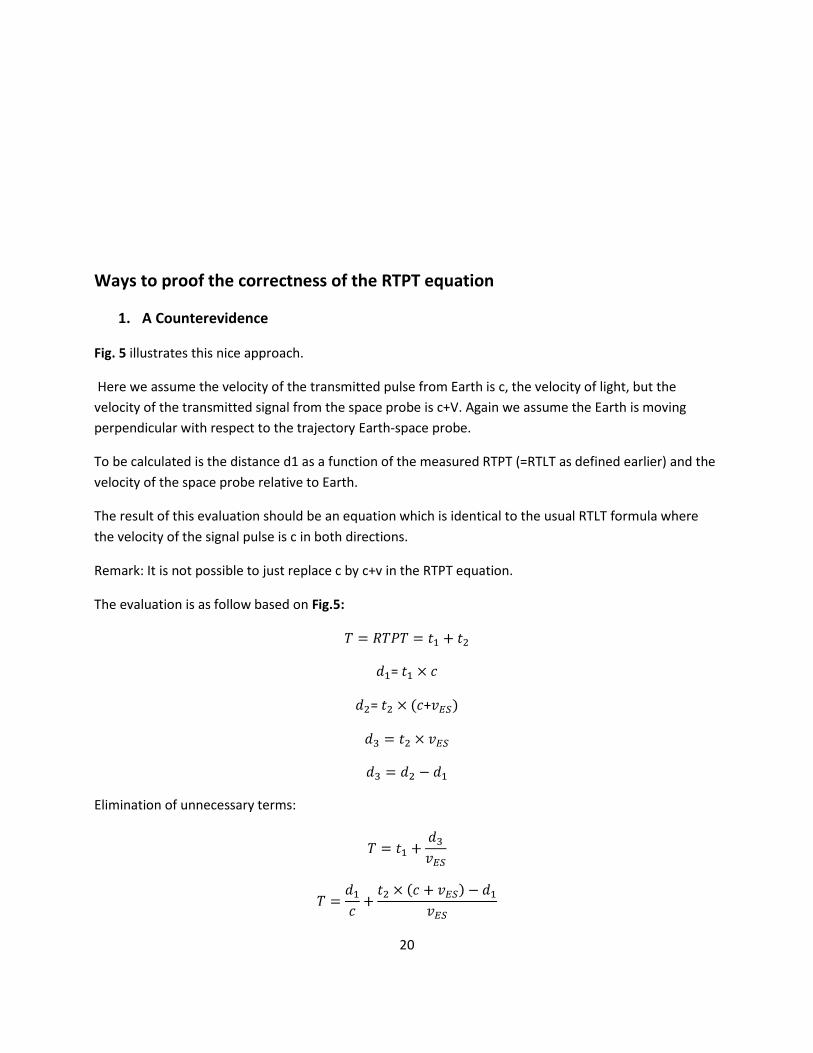
Ways to proof the correctness of the RTPT equation

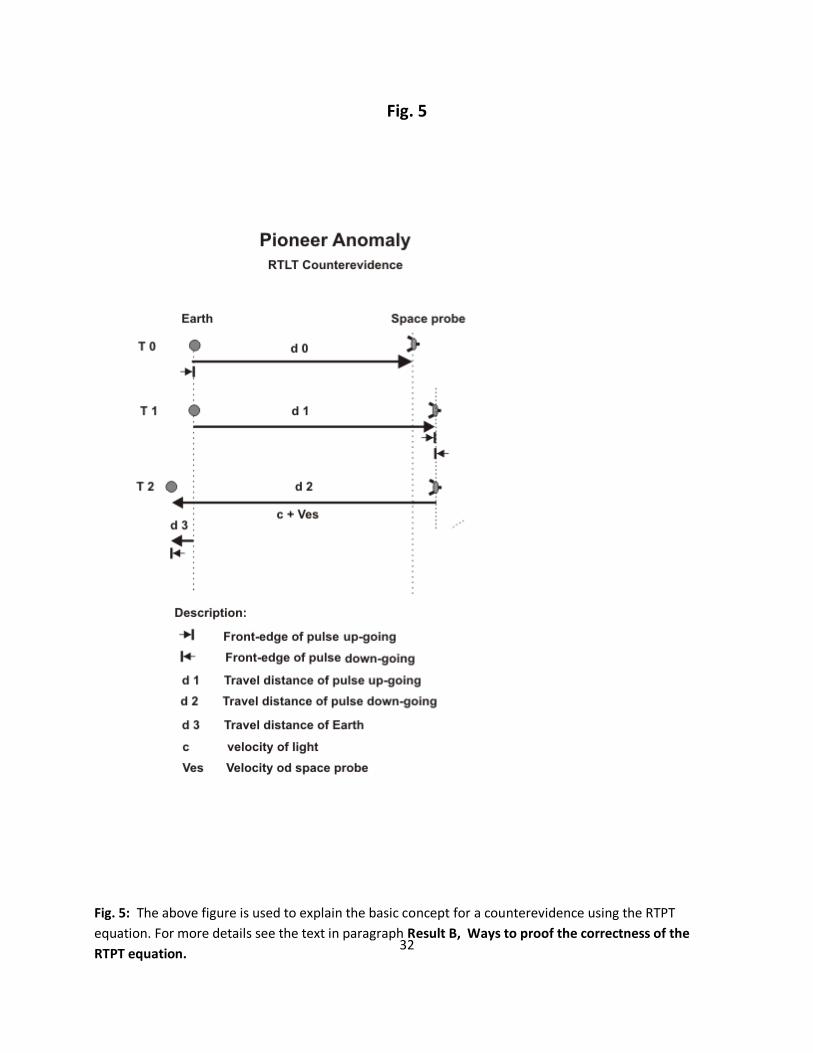
1. A Counterevidence

Fig. 5 illustrates this nice approach.

Here we assume the velocity of the transmitted pulse from Earth is c, the velocity of light, but the

velocity of the transmitted signal from the space probe is c+V. Again we assume the Earth is moving

perpendicular with respect to the trajectory Earth-space probe.

To be calculated is the distance d1 as a function of the measured RTPT (=RTLT as defined earlier) and the

velocity of the space probe relative to Earth.

The result of this evaluation should be an equation which is identical to the usual RTLT formula where

the velocity of the signal pulse is c in both directions.

Remark: It is not possible to just replace c by c+v in the RTPT equation.

The evaluation is as follow based on Fig.5:

=

= +

Elimination of unnecessary terms:

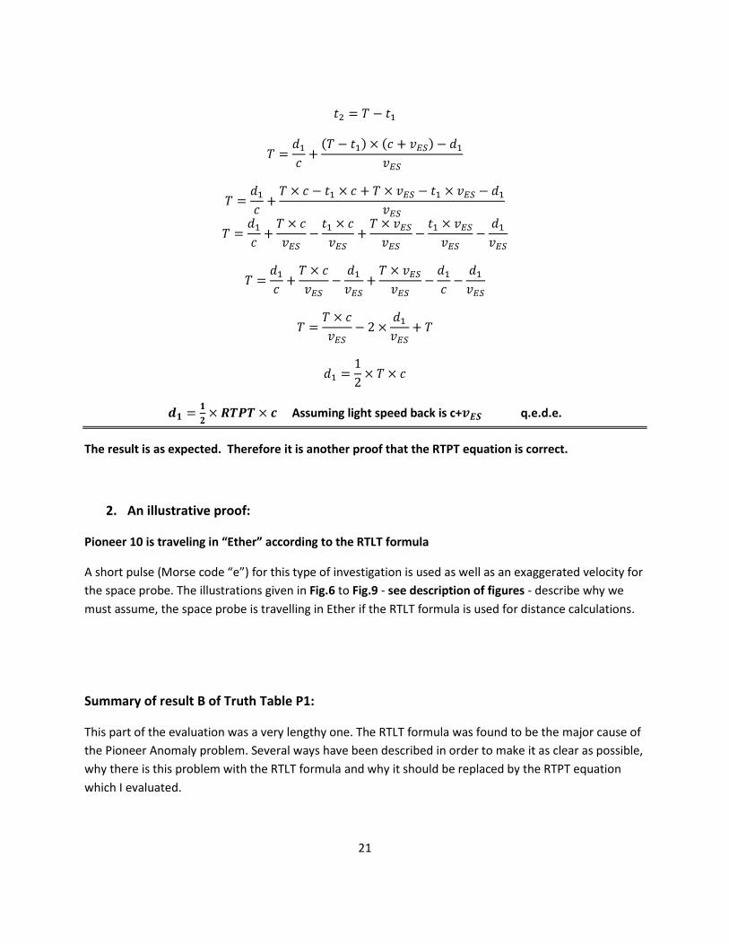
21

Assuming light speed back is c+ q.e.d.e.

The result is as expected. Therefore it is another proof that the RTPT equation is correct.

2. An illustrative proof:

Pioneer 10 is traveling in “Ether” according to the RTLT formula

A short pulse (Morse code “e”) for this type of investigation is used as well as an exaggerated velocity for

the space probe. The illustrations given in Fig.6 to Fig.9 - see description of figures - describe why we

must assume, the space probe is travelling in Ether if the RTLT formula is used for distance calculations.

Summary of result B of Truth Table P1:

This part of the evaluation was a very lengthy one. The RTLT formula was found to be the major cause of

the Pioneer Anomaly problem. Several ways have been described in order to make it as clear as possible,

why there is this problem with the RTLT formula and why it should be replaced by the RTPT equation

which I evaluated.

22

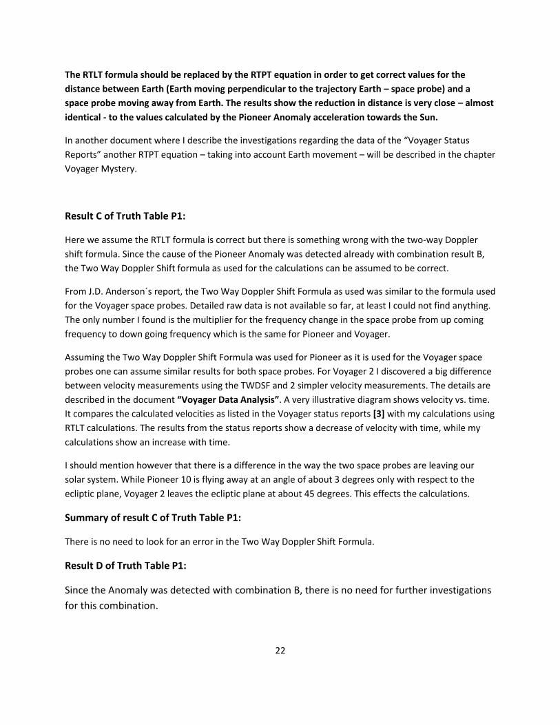
The RTLT formula should be replaced by the RTPT equation in order to get correct values for the

distance between Earth (Earth moving perpendicular to the trajectory Earth – space probe) and a

space probe moving away from Earth. The results show the reduction in distance is very close – almost

identical - to the values calculated by the Pioneer Anomaly acceleration towards the Sun.

In another document where I describe the investigations regarding the data of the “Voyager Status

Reports” another RTPT equation – taking into account Earth movement – will be described in the chapter

Voyager Mystery.

Result C of Truth Table P1:

Here we assume the RTLT formula is correct but there is something wrong with the two-way Doppler

shift formula. Since the cause of the Pioneer Anomaly was detected already with combination result B,

the Two Way Doppler Shift formula as used for the calculations can be assumed to be correct.

From J.D. Anderson´s report, the Two Way Doppler Shift Formula as used was similar to the formula used

for the Voyager space probes. Detailed raw data is not available so far, at least I could not find anything.

The only number I found is the multiplier for the frequency change in the space probe from up coming

frequency to down going frequency which is the same for Pioneer and Voyager.

Assuming the Two Way Doppler Shift Formula was used for Pioneer as it is used for the Voyager space

probes one can assume similar results for both space probes. For Voyager 2 I discovered a big difference

between velocity measurements using the TWDSF and 2 simpler velocity measurements. The details are

described in the document “Voyager Data Analysis”. A very illustrative diagram shows velocity vs. time.

It compares the calculated velocities as listed in the Voyager status reports [3] with my calculations using

RTLT calculations. The results from the status reports show a decrease of velocity with time, while my

calculations show an increase with time.

I should mention however that there is a difference in the way the two space probes are leaving our

solar system. While Pioneer 10 is flying away at an angle of about 3 degrees only with respect to the

ecliptic plane, Voyager 2 leaves the ecliptic plane at about 45 degrees. This effects the calculations.

Summary of result C of Truth Table P1:

There is no need to look for an error in the Two Way Doppler Shift Formula.

Result D of Truth Table P1:

Since the Anomaly was detected with combination B, there is no need for further investigations

for this combination.

23

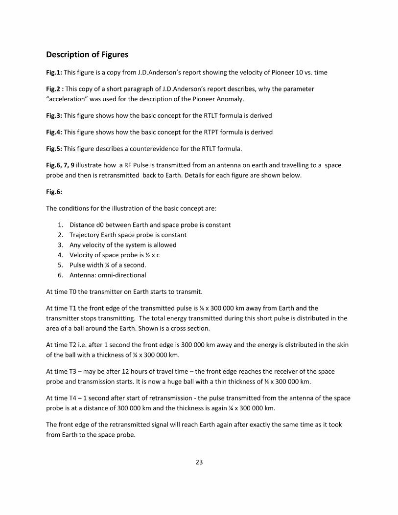
Description of Figures

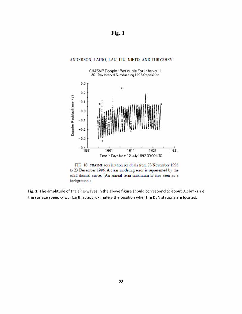
Fig.1: This figure is a copy from J.D.Anderson’s report showing the velocity of Pioneer 10 vs. time

Fig.2 : This copy of a short paragraph of J.D.Anderson’s report describes, why the parameter

“acceleration” was used for the description of the Pioneer Anomaly.

Fig.3: This figure shows how the basic concept for the RTLT formula is derived

Fig.4: This figure shows how the basic concept for the RTPT formula is derived

Fig.5: This figure describes a counterevidence for the RTLT formula.

Fig.6, 7, 9 illustrate how a RF Pulse is transmitted from an antenna on earth and travelling to a space

probe and then is retransmitted back to Earth. Details for each figure are shown below.

Fig.6:

The conditions for the illustration of the basic concept are:

1. Distance d0 between Earth and space probe is constant

2. Trajectory Earth space probe is constant

3. Any velocity of the system is allowed

4. Velocity of space probe is ½ x c

5. Pulse width ¼ of a second.

6. Antenna: omni-directional

At time T0 the transmitter on Earth starts to transmit.

At time T1 the front edge of the transmitted pulse is ¼ x 300 000 km away from Earth and the

transmitter stops transmitting. The total energy transmitted during this short pulse is distributed in the

area of a ball around the Earth. Shown is a cross section.

At time T2 i.e. after 1 second the front edge is 300 000 km away and the energy is distributed in the skin

of the ball with a thickness of ¼ x 300 000 km.

At time T3 – may be after 12 hours of travel time – the front edge reaches the receiver of the space

probe and transmission starts. It is now a huge ball with a thin thickness of ¼ x 300 000 km.

At time T4 – 1 second after start of retransmission - the pulse transmitted from the antenna of the space

probe is at a distance of 300 000 km and the thickness is again ¼ x 300 000 km.

The front edge of the retransmitted signal will reach Earth again after exactly the same time as it took

from Earth to the space probe.

24

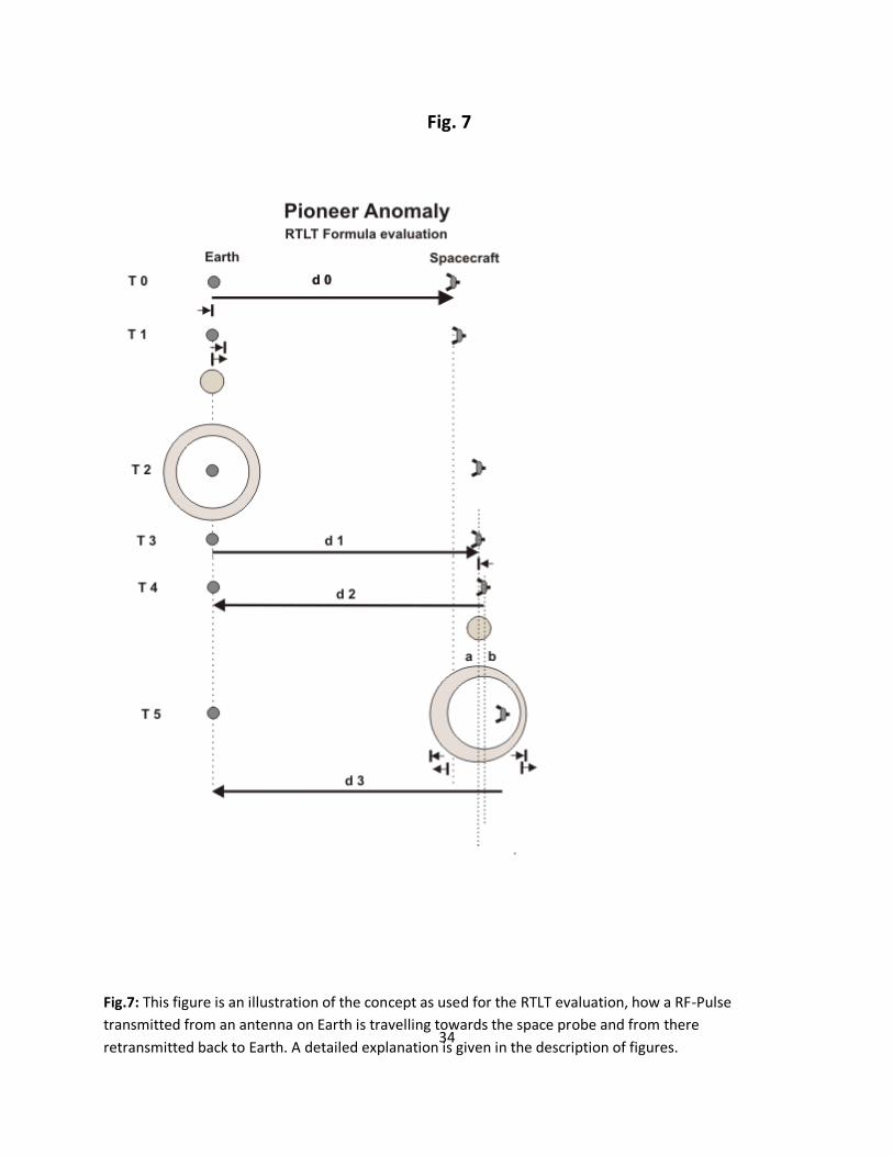
Fig.7:

The conditions for the illustration as used for the RTLT formula evaluation are:

1. Distance between Earth and space probe is not constant

2. Trajectory Earth space probe is constant

3. Velocity of space probe is constant (for Pioneer about 12 km/s)

4. Pulse width ¼ of a second.

5. Antenna: omni-directional

At time T0 the transmitter on Earth starts to transmit. Distance Earth to space probe is d0.

At time T1 the front edge of the transmitted pulse is ¼ x 300 000 km away from Earth and the

transmitter stops transmitting. The total energy transmitted during this short pulse is distributed in the

area of a ball around the Earth. Shown is a cross section. Distance is d1 (d0 + 1/4 x c)

At time T2 i.e. after 1 second the front edge is 300 000 km away and the energy is distributed in the skin

of the ball with a thickness of ¼ x 300 000 km.

At time T3 – may be after 12 hours of travel time – the front edge reaches the receiver of the space

probe and retransmission starts. It is now a huge ball with a skin thickness of ¼ x 300 000 km.

At time T4 – ¼ of a second after start of retransmission – the front end of the pulse transmitted from the

antenna of the space probe is at a distance of 300 000 km from the position where the space probe was

at time T3. The total energy transmitted during this short pulse is distributed in the area of a ball around

the space probe. The space probe is at this time at distance d2 (d1 + 1/4 x c). Retransmission stops at the

time the space probe has reached distance d2.

At time T5 – 1 second after start of retransmission - the pulse transmitted from the antenna of the space

probe is at a distance of 300 000 km and the shape of the skin looks like in the illustration. It is not a skin

of a perfect ball. The thickness towards Earth is ¼ x 300 000 km + d2-d1.

The front edge of the retransmitted signal will reach Earth again after exactly the same time as it took

from Earth to the space probe. Therefore it seems, as if the RTLT formula is correct.

The exaggerated velocity of the space probe pronounces how the shape of the cross section through the

ball around the space probe looks like.The illustration can be compared with the illustration how a sound

pulse is travelling in air.

25

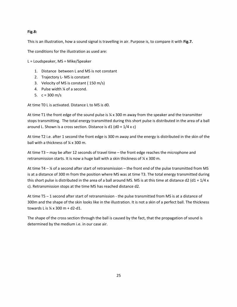
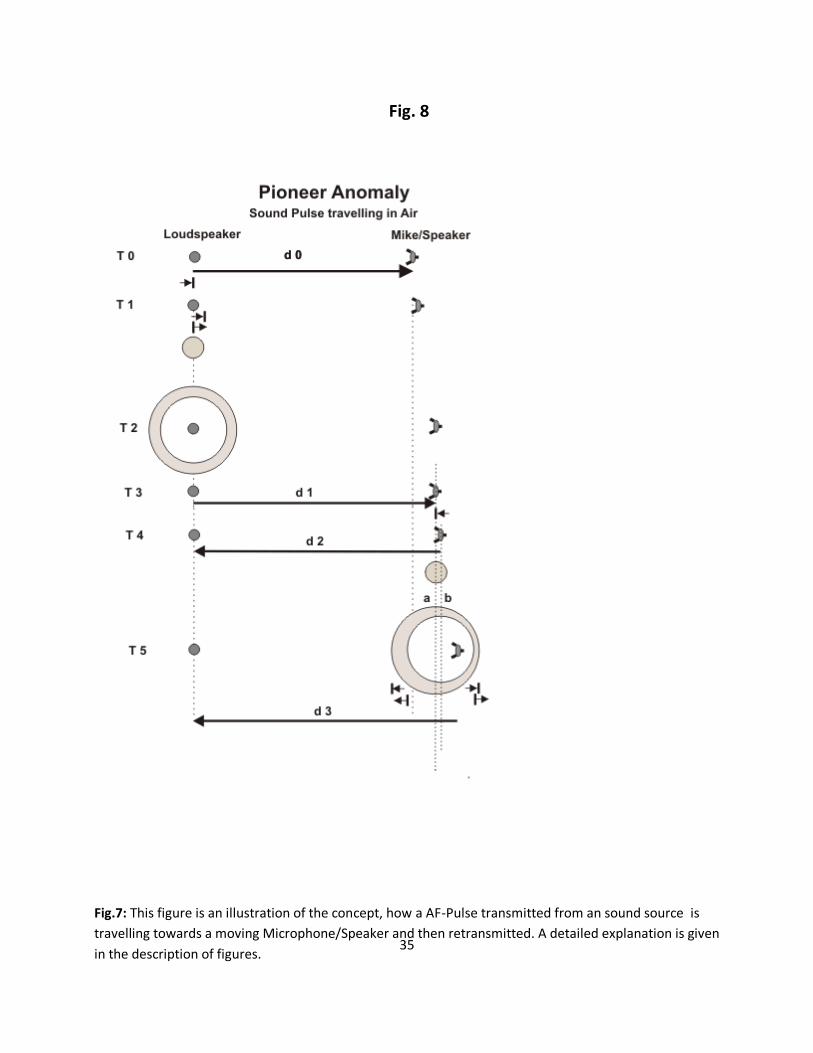
Fig.8:

This is an illustration, how a sound signal is travelling in air. Purpose is, to compare it with Fig.7.

The conditions for the illustration as used are:

L = Loudspeaker, MS = Mike/Speaker

1. Distance between L and MS is not constant

2. Trajectory L- MS is constant

3. Velocity of MS is constant ( 150 m/s)

4. Pulse width ¼ of a second.

5. c = 300 m/s

At time T0 L is activated. Distance L to MS is d0.

At time T1 the front edge of the sound pulse is ¼ x 300 m away from the speaker and the transmitter

stops transmitting. The total energy transmitted during this short pulse is distributed in the area of a ball

around L. Shown is a cross section. Distance is d1 (d0 + 1/4 x c)

At time T2 i.e. after 1 second the front edge is 300 m away and the energy is distributed in the skin of the

ball with a thickness of ¼ x 300 m.

At time T3 – may be after 12 seconds of travel time – the front edge reaches the microphone and

retransmission starts. It is now a huge ball with a skin thickness of ¼ x 300 m.

At time T4 – ¼ of a second after start of retransmission – the front end of the pulse transmitted from MS

is at a distance of 300 m from the position where MS was at time T3. The total energy transmitted during

this short pulse is distributed in the area of a ball around MS. MS is at this time at distance d2 (d1 + 1/4 x

c). Retransmission stops at the time MS has reached distance d2.

At time T5 – 1 second after start of retransmission - the pulse transmitted from MS is at a distance of

300m and the shape of the skin looks like in the illustration. It is not a skin of a perfect ball. The thickness

towards L is ¼ x 300 m + d2-d1.

The shape of the cross section through the ball is caused by the fact, that the propagation of sound is

determined by the medium i.e. in our case air.

26

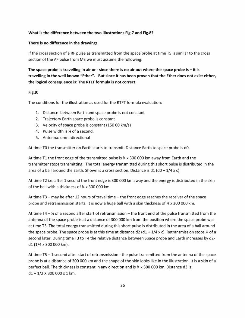
What is the difference between the two illustrations Fig.7 and Fig.8?

There is no difference in the drawings.

If the cross section of a RF pulse as transmitted from the space probe at time T5 is similar to the cross

section of the AF pulse from MS we must assume the following:

The space probe is travelling in air or - since there is no air out where the space probe is – it is

travelling in the well known “Ether”. But since it has been proven that the Ether does not exist either,

the logical consequence is: The RTLT formula is not correct.

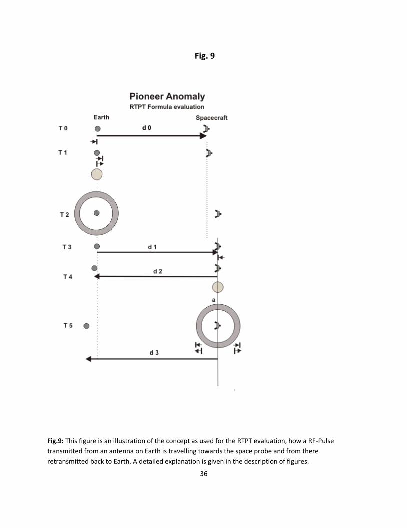
Fig.9:

The conditions for the illustration as used for the RTPT formula evaluation:

1. Distance between Earth and space probe is not constant

2. Trajectory Earth space probe is constant

3. Velocity of space probe is constant (150 00 km/s)

4. Pulse width is ¼ of a second.

5. Antenna: omni-directional

At time T0 the transmitter on Earth starts to transmit. Distance Earth to space probe is d0.

At time T1 the front edge of the transmitted pulse is ¼ x 300 000 km away from Earth and the

transmitter stops transmitting. The total energy transmitted during this short pulse is distributed in the

area of a ball around the Earth. Shown is a cross section. Distance is d1 (d0 + 1/4 x c)

At time T2 i.e. after 1 second the front edge is 300 000 km away and the energy is distributed in the skin

of the ball with a thickness of ¼ x 300 000 km.

At time T3 – may be after 12 hours of travel time – the front edge reaches the receiver of the space

probe and retransmission starts. It is now a huge ball with a skin thickness of ¼ x 300 000 km.

At time T4 – ¼ of a second after start of retransmission – the front end of the pulse transmitted from the

antenna of the space probe is at a distance of 300 000 km from the position where the space probe was

at time T3. The total energy transmitted during this short pulse is distributed in the area of a ball around

the space probe. The space probe is at this time at distance d2 (d1 + 1/4 x c). Retransmission stops ¼ of a

second later. During time T3 to T4 the relative distance between Space probe and Earth increases by d2-

d1 (1/4 x 300 000 km).

At time T5 – 1 second after start of retransmission - the pulse transmitted from the antenna of the space

probe is at a distance of 300 000 km and the shape of the skin looks like in the illustration. It is a skin of a

perfect ball. The thickness is constant in any direction and is ¼ x 300 000 km. Distance d3 is

d1 + 1/2 X 300 000 x 1 km.

27

The front edge of the retransmitted signal under these conditions will reach Earth after a time which is

greater than the time it took the signal to reach the space probe.

The exaggerated velocity of the space probe pronounces how the shape of the cross section through the

ball around the space probe looks like. The illustration can be compared with the illustration as shown

for the RTLT evaluation in Fig.7. Now we can say: There is no air and there is no “Ether” around the area

in which the nice space probe is travelling. Therefore my conclusion is: The RTPT equation is correct.

General remarks to the shape of the transmitted signal:

The shape is always a skin of a perfect ball.

The thickness is constant every where and depends on the pulse width only.

The energy density within the skin is dependent on the directivity of the antenna used.

For an omni–directional antenna, the cross section looks like shown in the figures.

If a high gain antenna is used, the shade of the ring in the drawings would be dark in direction of the

receiving station and basically empty within the rest of the ring. But it will be a perfect ring of equal

thickness.

28

Fig. 1

Fig. 1: The amplitude of the sine-waves in the above figure should correspond to about 0.3 km/s i.e.

the surface speed of our Earth at approximately the position wher the DSN stations are located.

29

Fig. 2

Fig. 2: The above figure is a copy oft he paragraph where the reason for choosing „acceleration“ as

the cause fort he Pioneer Anomaly is explained.

30

Fig. 3

Fig. 3: The above figure is used to explain the basic concept how the RTLT Formula is derived. For more

details see the text in paragraph Result B.

31

Fig. 4

Fig.4: The above figure is used to explain the basic concept how the RTPT Equation has been derived.

For more details see the text in paragraph Result B.

32

Fig. 5

Fig. 5: The above figure is used to explain the basic concept for a counterevidence using the RTPT

equation. For more details see the text in paragraph Result B, Ways to proof the correctness of the

RTPT equation.

33

Fig. 6

Fig.6: This figure is an illustration of the basic concept, how a RF-Pulse transmitted from an antenna on

Earth is travelling towards the space probe and from there retransmitted back to Earth. A detailed

explanation is given in the description of figures.

34

Fig. 7

Fig.7: This figure is an illustration of the concept as used for the RTLT evaluation, how a RF-Pulse

transmitted from an antenna on Earth is travelling towards the space probe and from there

retransmitted back to Earth. A detailed explanation is given in the description of figures.

35

Fig. 8

Fig.7: This figure is an illustration of the concept, how a AF-Pulse transmitted from an sound source is

travelling towards a moving Microphone/Speaker and then retransmitted. A detailed explanation is given

in the description of figures.

36

Fig. 9

Fig.9: This figure is an illustration of the concept as used for the RTPT evaluation, how a RF-Pulse

transmitted from an antenna on Earth is travelling towards the space probe and from there

retransmitted back to Earth. A detailed explanation is given in the description of figures.

37

The IME Experiment

In the first part of this document I described how the famous Pioneer Anomaly problem could be solved.

The best way to proof a theory is to perform an experiment. Part two of this document describes briefly

such an experiment. The IME-Experiment I propose is an experiment which will proof that the RTPT

equation to calculate the distance of a space probe should be used instead of the RTLT formula. IME

stands for ISS-Mars-Earth. The experiment can be performed by radio amateurs. There are always

amateur radio operators on board of ISS. The amateur radio community plans to have a station on Mars.

The basic concept of the experiment is as follows:

Morse code signals are used for the experiment. Time controlled signals are sent simultaneously from ISS

as well as from Earth to a receiver on Mars. The received signals on Mars will detect, if the signals arrive

at the predicted time. If planet Mars is far enough away, the signals can be identified as Morse code

letters at a relatively high speed of about 500 words per minute. The proposed timing is such, that two

letters will be received on Mars if the experiment is successful, i.e. the RTPT equation is correct (either

“t” and “a” resp. “n” and “t” depending on the direction ISS is flying). If the experiment fails, i.e. the RTLT

formula is correct, the received signal will result in a received letter “k”. The result of the experiment can

actually be made audible. After retransmission from Mars, conversion to an audible frequency and

slowing down the relatively high Morse speed even people without any practical Morse code

background could identify the result.

A detailed description of this proposed experiment will be published in the German Radio Amateur

Magazine “Funkamateur”.

38

Acknowledgements

Thanks go to Klaus Mischke who introduced me to the Pioneer Anomaly and to Uli Diebold who

extracted the Voyager data from the Voyager Status Reports so I could use them in spread sheet

calculations. And special thanks to Dr.Natalia E. Papitasvilli for her assistance to find all the

interesting links with helpful data.

Over all summary

According to my evaluation, the reason for the discovery of the Pioneer Anomaly lies in the

usage of a wrong formula – the RTLT formula - to calculate the distance of a moving object in

space.

The reduction in distance within 15 years of travel time for Pioneer 10 was calculated to be

about 100 000 km using the proposed acceleration towards the Sun.

Applying the new RTPT equation to calculate the distance reduction gives exactly the values as

has been calculated by J.D.Anderson.

Final remark:

The readers of this document will certainly look for errors and mistakes in my evaluation and I

would not be bothered too much if I really made some mistakes. It was an interesting task. And

if every thing I calculated is wrong, we will have further room for nice and interesting

speculations what is causing this famous anomaly. And we will have this nice comet with two

apogees .There is however a problem: Since I have never made a single mistake in my whole

life, my calculations might be correct after all…….hi.

39

Literature and Links

[1] Study of the anomalous acceleration of Pioneer 10 and 11 John D. Anderson et al. Dated: 11 April 2002

The article which describes in detail the Pioneer space probes and the famous Pioneer

Anomaly Problem

[2] http://omniweb.gsfc.nasa.gov/egi/models/helios.cgil

A link to detailed data for space probes.

http://www2.jpl.nasa.gov/basics/bsf13-1.htmll

Chapter 13: Spacecraft Navigation. The meaningful measurements of a spacecraft´s motion.

[3] http://voyager.jpl.nasa.gov/mission/weekly-reports/

The link where Range, Velocity and Round Trip Light Time Data can be found for

Voyager 1 and 2

[4] www.safog.com/home/pioneer_anomalie.html

Another detailed description of the anomaly problem

[5] http://de.wikipedia.org/wiki/Pioneer-Anomalie

Here the deviation of 100 000 km within 15 years of travel time is mentioned

[6] http://www.mpifr-bonn.de/staff/sbritzen/soso09_konstanten.pdf

Here the deviation of 100 000 km within 15 years of travel time is mentioned

40

Usage of the RTPT equation in other areas

Distance of a far away Quasar

Conditions:

Distance d: 50 x 10E7 Light years

Hubble Constant: 75 / km x Mpc

The following trick is used to calculate the actual distance:

A pulse was sent from Earth 100 x 10E7 years ago to the Quasar. The velocity of the Quasar

away from Earth was calculated to be 11 500 km/s.

Using the RTPT equation to calculate the distance gives a reduction in distance of about 5 Mpc.

Distance of an object with V approaching c.

The distance at the time the pulse has reached the object – quite some time ago - becomes

zero, the object must have originated on Earth……..most probably in Bavaria.