
Knots, Graphs and Geometry Graphs and Geometry Abhijit Champanerkar Department of Mathematics,...
45
Knots, Graphs and Geometry Abhijit Champanerkar Department of Mathematics, College of Staten Island, CUNY Mathematics Program, The Graduate Center, CUNY GC MathFest 2014 Nov 11, 2014
-
Upload
truongkhanh -
Category
Documents
-
view
214 -
download
0
Transcript of Knots, Graphs and Geometry Graphs and Geometry Abhijit Champanerkar Department of Mathematics,...

Knots, Graphs and Geometry
Abhijit Champanerkar
Department of Mathematics,College of Staten Island, CUNY
Mathematics Program,The Graduate Center, CUNY
GC MathFest 2014Nov 11, 2014

What is a knot ?
A knot is a (smooth) embedding of the circle S1 in S3. Similarly, alink of k-components is a (smooth) embedding of a disjoint unionof k circles in S3.
Figure-8 knot Whitehead link Borromean rings
Two knots are equivalent if there is continuous deformation(ambient isotopy) of S3 taking one to the other.
Goals: To classify knots upto equivalence.
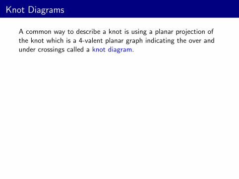
Knot Diagrams
A common way to describe a knot is using a planar projection ofthe knot which is a 4-valent planar graph indicating the over andunder crossings called a knot diagram.
A given knot has manydifferent diagrams.
Two knot diagrams representthe same knot if and only ifthey are related by a sequenceof three kinds of moves onthe diagram called theReidemeister moves.

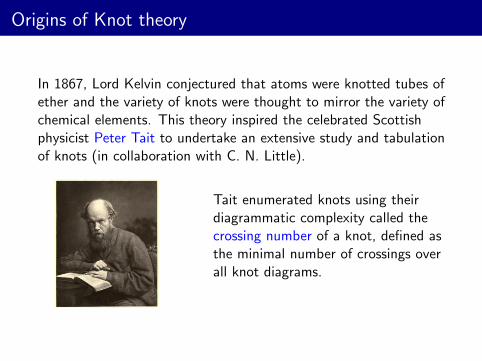
Origins of Knot theory
In 1867, Lord Kelvin conjectured that atoms were knotted tubes ofether and the variety of knots were thought to mirror the variety ofchemical elements. This theory inspired the celebrated Scottishphysicist Peter Tait to undertake an extensive study and tabulationof knots (in collaboration with C. N. Little).
Tait enumerated knots using theirdiagrammatic complexity called thecrossing number of a knot, defined asthe minimal number of crossings overall knot diagrams.

Knots with low crossing number

Tait Conjectures
A knot diagram is alternating if the crossings alternate under, over,under, over, as one travels along each component of the link. Aknot is alternating if it has an alternating diagram.
A reduced diagram is a diagramwith no reducible crossings.
Tait Conjecture 1 Any reduced diagram of an alternating link hasthe fewest possible crossings.
Tait made more conjectures, about relating alternating diagrams(Flyping Conjecture), and about writhe of alternating knots.

Knot invariants
How to tell knots apart ?
A knot invariant is a “quantity” that is equal for equivalent knots,independent of the description, hence can be used to tell knotsapart
Knot invariants have many different forms e.g. numbers,polynomials, groups etc and are defined using techniques fromdifferent fields e.g. topology, graph theory, geometry, algebraicgeometry, representation theory etc.
The crossing number is a knot invariant, however very hard tocompute. Tait Conjecture 1 gives a way to compute it foralternating knots.

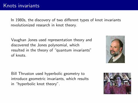
Knots invariants
In 1980s, the discovery of two different types of knot invariantsrevolutionized research in knot theory.
Vaughan Jones used representation theory anddiscovered the Jones polynomial, whichresulted in the theory of “quantum invariants”of knots.
Bill Thruston used hyperbolic geometry tointroduce geometric invariants, which resultsin “hyperbolic knot theory”.

Examples of knots invariants
I Topological: Arising from topology of the S3 − K e.g.Fundamental group, Alexander polynomial (1927), Seifertsurfaces (1934), Knot Heegaard Floer homology(Ozsvath-Szabo-Rasmussen, 2003).
I Diagrammatic: Fox n-colorings (Fox, 1956), Jones polynomial(1984), Kauffman bracket (1987), Khovanov homology(1999), Turaev genus (2006).
I Geometric: Arising from the hyperbolic geometry of S3 − K :volume, cusp shape, invariant trace field, character variety,A-polynomial (1994).
A big problem in knot theory is to relate different kind ofinvariants.

Knots and Graphs
The Tait graph GK of a knot diagram K is a plane signed grapharising from a checkboard coloring of K as follows: shaded regionscorrespond to vertices , crossings corresponding to signed edges.
The other checkboard coloring gives the planar dual of GK .

Knots and Graphs
The Tait graph GK of a knot diagram K is a plane signed grapharising from a checkboard coloring of K as follows: shaded regionscorrespond to vertices , crossings corresponding to signed edges.
The other checkboard coloring gives the planar dual of GK .

Knots and Graphs
Thistlethwaite (1987)(1) Jones polynomial of K can be written in terms of spanning
trees of GK : VK (t) =∑
T⊂GK
µ(T ).
(2) If K is connected, reduced alternating diagram thenspanVK (t) = c(K )
Corollary(1) Proves Tait Conjecture 1.(2) If K is connected, reduced alternating diagram, Knotdeterminant det(K ) = number of spanning trees of GK .

Knots and Graphs
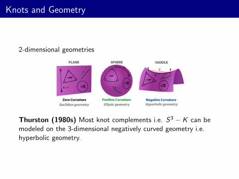
Knots and Geometry
2-dimensional geometries
Thurston (1980s) Most knot complements i.e. S3 − K can bemodeled on the 3-dimensional negatively curved geometry i.e.hyperbolic geometry.

Basic hyperbolic geometry I
Escher’s work using hyperbolic plane Hyperbolic plane crochet by Daina Taimina
Hyperbolic upper-half plane Hyperbolic upper-half space

Basic hyperbolic geometry I
Escher’s work using hyperbolic plane Hyperbolic plane crochet by Daina Taimina
Hyperbolic upper-half plane Hyperbolic upper-half space

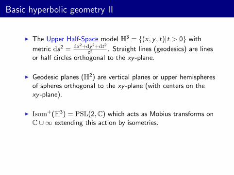
Basic hyperbolic geometry II
I The Upper Half-Space model H3 = {(x , y , t)|t > 0} with
metric ds2 = dx2+dy2+dt2
t2. Straight lines (geodesics) are lines
or half circles orthogonal to the xy -plane.
I Geodesic planes (H2) are vertical planes or upper hemispheresof spheres orthogonal to the xy -plane (with centers on thexy -plane).
I Isom+(H3) = PSL(2,C) which acts as Mobius transforms onC ∪∞ extending this action by isometries.
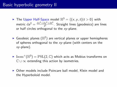
I Other models include Poincare ball model, Klein model andthe Hyperboloid model.

Basic hyperbolic geometry II
I The Upper Half-Space model H3 = {(x , y , t)|t > 0} with
metric ds2 = dx2+dy2+dt2
t2. Straight lines (geodesics) are lines
or half circles orthogonal to the xy -plane.
I Geodesic planes (H2) are vertical planes or upper hemispheresof spheres orthogonal to the xy -plane (with centers on thexy -plane).
I Isom+(H3) = PSL(2,C) which acts as Mobius transforms onC ∪∞ extending this action by isometries.
I Other models include Poincare ball model, Klein model andthe Hyperboloid model.

Hyperbolic building blocks
How to build hyperbolic knots or manifolds ?
Ideal tetrahedra & polyhedra in hyperbolic 3-space can be gluedtogether to make knot complements. This is a geometric way ofdescribing knots.
The least number of hyperbolic tetrahedra gives a geometriccomplexity for knots.

Hyperbolic building blocks
How to build hyperbolic knots or manifolds ?
Ideal tetrahedra & polyhedra in hyperbolic 3-space can be gluedtogether to make knot complements. This is a geometric way ofdescribing knots.
The least number of hyperbolic tetrahedra gives a geometriccomplexity for knots.
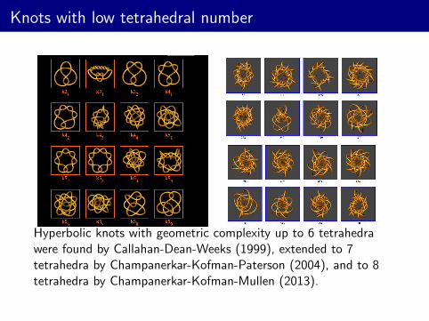
Knots with low tetrahedral number
Hyperbolic knots with geometric complexity up to 6 tetrahedrawere found by Callahan-Dean-Weeks (1999), extended to 7tetrahedra by Champanerkar-Kofman-Paterson (2004), and to 8tetrahedra by Champanerkar-Kofman-Mullen (2013).

Knots with low crossing number

Computing knot invariants
Many computer programs are available to compute knot invariants.
SnapPy by Culler and Dunfield, based onSnapPea by Jeff Weeks computes hyperbolicinvariants.
KnotTheory by Bar-Natan, is a Mathematicapackage which computes diagrammaticinvariants.

Computing knot invariants
Many computer programs are available to compute knot invariants.
SnapPy by Culler and Dunfield, based onSnapPea by Jeff Weeks computes hyperbolicinvariants.
KnotTheory by Bar-Natan, is a Mathematicapackage which computes diagrammaticinvariants.

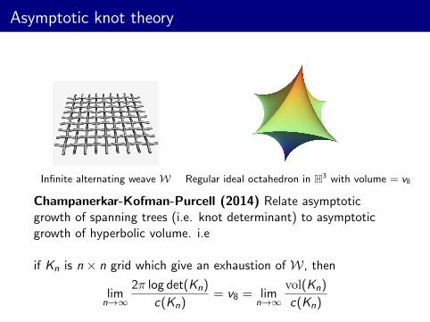
Asymptotic knot theory
Infinite alternating weave W Regular ideal octahedron in H3 with volume = v8
Champanerkar-Kofman-Purcell (2014) Relate asymptoticgrowth of spanning trees (i.e. knot determinant) to asymptoticgrowth of hyperbolic volume. i.e
if Kn is n × n grid which give an exhaustion of W, then
limn→∞
2π log det(Kn)
c(Kn)= v8 = lim
n→∞
vol(Kn)
c(Kn)
Abhijit’s Home page:http://www.math.csi.cuny.edu/abhijit/
KnotAtlas: http://katlas.math.toronto.edu/wiki/
SnapPy: http://www.math.uic.edu/~t3m/SnapPy/
Knot Invariants: http://www.indiana.edu/~knotinfo/
KnotPlot: http://www.knotplot.com/
Thank you


