Khalili, M., Brissette, F., Leconte, R., 2009, Stochastic Multi-Site ...

ORIGINAL PAPER

Stochastic multi-site generation of daily weather data

Malika Khalili Æ Francois Brissette ÆRobert Leconte

Published online: 7 October 2008

� Springer-Verlag 2008

Abstract Spatial autocorrelation is a correlation between

the values of a single variable, considering their geo-

graphical locations. This concept has successfully been

used for multi-site generation of daily precipitation data

(Khalili et al. in J Hydrometeorol 8(3):396–412, 2007).

This paper presents an extension of this approach. It aims

firstly to obtain an accurate reproduction of the spatial

intermittence property in synthetic precipitation amounts,

and then to extend the multi-site approach to the generation

of daily maximum temperature, minimum temperature and

solar radiation data. Monthly spatial exponential functions

have been developed for each weather station according to

the spatial dependence of the occurrence processes over the

watershed, in order to fulfill the spatial intermittence con-

dition in the synthetic time series of precipitation amounts.

As was the case for the precipitation processes, the multi-

site generation of daily maximum temperature, minimum

temperature and solar radiation data is realized using spa-

tially autocorrelated random numbers. These random

numbers are incorporated into the weakly stationary

generating process, as with the Richardson weather gen-

erator, and with no modifications made. Suitable spatial

autocorrelations of random numbers allow the reproduction

of the observed daily spatial autocorrelations and monthly

interstation correlations. The Peribonca River Basin

watershed is used to test the performance of the proposed

approaches. Results indicate that the spatial exponential

functions succeeded in reproducing an accurate spatial

intermittence in the synthetic precipitation amounts. The

multi-site generation approach was successfully applied for

the weather data, which were adequately generated, while

maintaining efficient daily spatial autocorrelations and

monthly interstation correlations.

Keywords Weather generator �Multi-site � Precipitation �Temperature � Solar radiation

List of symbols

A matrix (3,3) whose elements are defined

from lag 0 and lag 1 serial and cross-

correlation coefficient matrices of observed

residuals

B matrix (3,3) whose elements are defined

from lag 0 and lag 1 serial and cross

correlation coefficient matrices of observed

residuals

F spatial exponential cumulative distribution

function

I Moran value

l total number of days in a given month

m total number of cTmax, cTmin or cSr values

taken from their range

M0 matrix of lag 0 serial and cross-correlations

M1 matrix of lag 1 serial and cross-correlations

M. Khalili (&)

Department of Civil Engineering and Applied Mechanics,

McGill University, 817, Sherbrooke Street West,

Montreal, QC H3A 2K6, Canada

e-mail: [email protected]

F. Brissette � R. Leconte

Ecole de technologie superieure, Quebec University,

1100, Notre-Dame Street West,

Montreal, QC H3C 1K3, Canada


R. Leconte


123

Stoch Environ Res Risk Assess (2009) 23:837–849

DOI 10.1007/s00477-008-0275-x

n total number of locations

rt(k) synthetic precipitation amount at site k on

day t

SDI spatial dependence indicator

uTmax (n, 1) vector of n independent and normally

distributed random numbers used for

maximum temperature

uTmin (n,1) vector of n independent and normally

distributed random numbers used for

minimum temperature

uSr (n,1) vector of n independent and normally

distributed random numbers used for solar

radiation

vt(k) uniform [0, 1] random number

VTmax(n, 1) vector of n spatially autocorrelated random

numbers used for maximum temperature

VTmin(n,1) vector of n spatially autocorrelated random

numbers used for mimimum temperature

VSr(n,1) vector of n spatially autocorrelated random

numbers used for solar radiation

wij spatial weight between two locations i and j

W(n,n) weight matrix

wmax maximum positive eigenvalue of W(n, n)

wmin largest negative eigenvalue of W(n, n) in

absolute value

X single variable

xi observed value at location i

�x average of the xi over n locations�Xk jð Þ mean of temperature or solar radiation

vp,k(j) matrix (3,1) of maximum temperature

(j = 1), minimum temperature (j = 2) and

solar radiation (j = 3) residuals for day k of

year p

kt(k) inverse of the precipitation mean at site k on

day t

rk(j) standard deviation of temperature or solar

radiation

ep,k(j) matrix (3, 1) of independent standard normal

random numbers N[0,1] for day k of year p

qvi;0 vj;0lag 0 cross-correlation coefficient between

the residuals of variable i and the residuals

of variable j

qvi;0 vj;�1lag 1 cross-correlation coefficient between

the current residuals of variable i and the

previous residuals of variable j

qvi;0 vi;�1lag 1 serial correlation of variable i

cTmax moving average coefficient used for

maximum temperature

cTmin moving average coefficient used for

minimum temperature

cSr moving average coefficient used for solar

radiation

1 Introduction

Weather generators are increasingly being used in a variety

of water resource studies due to their ability to provide

series of weather data for any length of time with similar

statistics as observations to which the weather generators

have been fitted. Richardson weather generator (WGEN)

(Richardson 1981; Richardson and Wright 1984) is the

most commonly used weather generator, and uses a first-

order two-state Markov chain model to generate precipi-

tation occurrences and distribution function, such as

gamma or exponential, to model precipitation amounts.

Another basic type of weather generator is the one by

Semenov and Barrow (1997), which uses semi-empirical

distributions to simulate precipitation processes. There are

also non-parametric weather generators (Brandsma and

Buishand 1997), which use the resampling of a weather

variables vector on a day of interest from the historical data

by conditioning on the simulated values of previous days.

These weather generators operate at a single site, and

thus fail to reproduce the spatial dependence present in the

observed data. In fact, the extension of the weather event

over the watershed implies that the weather data at a given

weather station is likely to be correlated with those in the

surrounding area. Further research has therefore been

conducted to develop multi-site weather generators, such as

space-time models (Bardossy and Plate 1992; Bogardi et al.

1993), which use the atmospheric circulation patterns with

conditional distributions and conditional spatial covariance

functions. Non-homogeneous hidden Markov model (Bel-

lone et al. 2000; Hughes and Guttorp 1994a, b; Hughes

et al. 1999) uses a discrete weather state to link the large

scale atmospheric measures and the small scale spatially

discontinuous precipitation field. A multi-site weather

generator based on a nearest-neighbor resampling from

historical data has been developed by Buishand and

Brandsma (2001). Wilks (1998) developed a multi-site

version of the Richardson weather generator based on

serially independent but spatially correlated random

numbers.

The multi-site weather generators presented above are

designed using relevant statistic information, but yield

difficulties in their implementation, and produce limited

results. Wilks (1998) proposes an interesting multi-site

framework using the Richardson model, but is unable to do

away with certain practical difficulties, such as the com-

putational burden and the correlation matrix positive

definiteness constraint. Wilks (1998) proposes also one

attempt to alleviate the spatial intermittence problem using

a 3-parameter mixed exponential, but further improve-

ments are required in this regard. An algorithm simplifying

the execution of Wilks’ approach has been developed by

838 Stoch Environ Res Risk Assess (2009) 23:837–849

123

Brissette et al. (2007), with a multi-exponential function to

improve the reproduction of seasonal spatial intermittence.

Tae-woong et al. (2007) used the Markovian model for

occurrence process as in wilks (1998), but the dependence

of occurrence is directly considered among stations using

space-time Markov model.

Regarding the multi-site generation of temperature and

solar radiation data, the main earlier approaches were those

developed by Wilks (1999) and Buishand and Brandsma

(2001). The first uses an extension of the weakly stationary

generating process from 3 to 3 k dimensions, where k is the

total number of locations. However, this extension yields

correlation matrices that are not easy to handle, particularly

for a large station network, and the coefficients of inter-

station correlations are not necessarily all significant. The

second approach uses historical data, which cannot deal

with climate change studies.

Multi-site generation approach of daily precipitation

data has been developed by Khalili et al. (2007). This

approach adopts the Richardson weather generator, and

uses the spatial autocorrelation concept to reproduce the

spatial dependence seen in georeferenced observations.

The core advantage of using spatial autocorrelation lies in

its ability to summarize the spatial dependence over a

watershed in a single number, which minimizes compu-

tation requirements, and highlights the straightforwardness

of the approach when used for a large data set. Using a

proper weight matrix, which is required for the computa-

tion of spatial autocorrelation, the multi-site approach can

reproduce observed daily spatial autocorrelations, and

implies the reproduction of observed monthly pairwise

correlations. The approach by Khalili et al. (2007) allows

an accurate simulation of precipitation processes, while

maintaining daily spatial autocorrelations and monthly

interstation correlations. However, while the simple

exponential distribution function used to model precipita-

tion amounts ensures a practically good fit with these

precipitation amounts, it fails to fulfill the spatial inter-

mittence property, which means that the precipitation

amounts at a given station depend on whether the sur-

rounding stations are wet or dry. It is thus not appropriate

to model the precipitation amounts at a given station

without considering the occurrence states in the sur-

rounding stations.

This paper focuses firstly on improving the simulation of

precipitation amounts in order to obtain an accurate

reproduction of daily spatial intermittence using spatial

autocorrelation concept. Secondly, it examines the use of

spatial autocorrelation for a straightforward multi-site

generation of daily temperature and solar radiation data.

The next section presents a definition of spatial autocor-

relation. Section 3 presents the general theory of stochastic

multi-site generation approach of daily precipitation data

(Khalili et al. 2007) and the suggested method for

improving the spatial intermittence of precipitation

amounts. The proposed methodology for multi-site gener-

ation of daily temperature and solar radiation data is

described in Sect. 4. Section 5 presents and discuses the

results of the proposed approaches.

2 Definition of spatial autocorrelation

Spatial autocorrelation is a correlation among the values of

a single variable, taking into account their arrangement in

geographic space (Griffith 2003). This statistic complies

with the first law of geography mentioned by Tobler (1970)

‘‘Everything is related to everything else, but near things

are more related than distant things’’. A more useful

spatial autocorrelation statistic is Moran’s I (Moran 1950;

Odland 1988; Griffith 2003), presented as:

I ¼Pn

i¼1 xi � �xð ÞPn

j¼1 wij xj � �x� �.Pn

i¼1

Pnj¼1 wij

Pni¼1 xi � �xð Þ2=n

ð1Þ

where xi denotes the observed value of a single variable X at

location i, �x is the average of the xi over n locations, and wij

is the spatial weight between two locations i and j. In the

matrix form of the right side of Eq. 1, all weights are stored

within the spatial weight matrix W(n, n). Usually, this

matrix may be in a row-standardized form, which means

that all weights in a row will sum up to 1. If the weight

matrix is used without row-standardization, this does not

change the degree of spatial autocorrelation. In fact, to

compensate for the effect of the non-row-standardization

form, the term nPn

i¼1

Pn

j¼1wij

in Moran’s I expression will not

be equal to 1 as it is when each row sums to 1.

It should be noted that Moran’s I computes the depen-

dence among values of a single variable, which are

weighted according to their locations respective to each

other. It therefore differs from the Pearson product moment

correlation coefficient, which measures the relation

between two variables without weight parameters. In pre-

cipitation context, the single variable X used in Moran’s I

(Eq. 1) represents the values of the precipitation processes

observed at the set of stations on a given day as:

X ¼ x1; :::; xn½ � ð2Þ

According to the precipitation process to be generated,

the xi may be either the occurrence state at location i or the

precipitation amount. For the occurrence process, the value

0 is assigned to the dry state and 1 to the wet state

considered as the state of at least 0.254 mm of precipitation

amount.

Moran’s I has an expected value of (-1/(n - 1))

(Moran 1950; Cliff and Ord 1981), and can vary between

Stoch Environ Res Risk Assess (2009) 23:837–849 839

123

-1 and 1 (Griffith 2003). When neighbouring values of a

sequenced variable tend to be similar, the resulting Mor-

an’s I will be larger than -1/(n - 1)), and the spatial

autocorrelation is said to be positive. When neighbouring

values tend to be dissimilar, the resulting Moran’s I will be

smaller than (-1/(n - 1)), and the spatial autocorrelation

is said to be negative. When these values are independent

over space, the Moran’s I will be equal to (-1/(n - 1)).

The spatial weight matrix is an important concept in the

analysis of spatial autocorrelation. The matrix has zero

diagonal elements because wii = 0 by convention, and there

are no restrictions on the off-diagonal elements. A wide

range of suggestions have been proposed in the literature

for specifying spatial weights (Odland 1988; Ullah and

Giles 1991; Anselin 1980; Murdoch et al. 1993). An

appropriate spatial weighting function can be selected

which assigns weights to each pair of locations. The value

of the spatial autocorrelation depends on the selected

weight matrix and on the observed data. The weight matrix

may not only be derived from the geographical informa-

tion, but also from other information describing the relation

between locations (Odland 1988). Khalili et al. (2007), in

their multi-site generation approach of daily precipitation

data, took advantage of this flexibility in defining the

spatial weight between each pair of stations to reproduce

not only the observed daily spatial autocorrelations over

the watershed, but also the monthly interstation

correlations.

3 Multi-site generation approach of daily precipitation

data

The multi-site generation approach of daily precipitation

data (Khalili et al. 2007) uses a spatial moving average

process to generate spatially autocorrelated random num-

bers, whose spatial autocorrelations can reproduce the

observed daily spatial autocorrelations in the synthetic time

series of precipitation occurrences and amounts. Spatially

autocorrelated random numbers are used in the Richardson

weather generator to simulate the precipitation occurrences

using the first-order Markov chain model.

Another set of spatially autocorrelated random numbers

was used to simulate the synthetic precipitation amounts by

inverting the simple exponential cumulative distribution

function. However, to reproduce adequate spatial inter-

mittence, it appears important to think about the

relationship between the precipitation amounts at a given

station and the occurrence states over the watershed before

setting out to model the precipitation amounts. This obvi-

ously highlights the potential of employing spatial

autocorrelation to investigate the spatial interaction

between the occurrence processes over the watershed.

Data from the Peribonca River Basin watershed is used

to carry out investigations to that effect. As anticipated,

relationship is found between the Moran values for

occurrence processes and the mean of precipitation

amounts at each station and month. Consequently, the

simple exponential distribution will be used, but with the

rate parameter, which represents the inverse of the pre-

cipitation mean, derived from these relationships.

Regression functions can be used to determine the mean of

precipitation amounts according to the spatial autocorre-

lation of the occurrence processes computed over the

watershed. In doing so, the resulting simple exponential

distribution will be called a spatial exponential distribu-

tion, in order to indicate that the mean of this distribution is

defined according to the spatial dependence of the occur-

rence states at the set of stations.

Furthermore, it may be interesting to suggest another

structure of spatial dependence by allowing the Moran’s I

to be computed without removing the average as:

SDI ¼Pn

i¼1 xi

Pnj¼1 wijxj

.Pni¼1

Pnj¼1 wij

Pni¼1 x2

i =nð3Þ

This formula, which provides positive and higher

values, appears to offer a more significant correlation

between the mean of precipitation amounts and the spatial

dependence of occurrence states. This spatial structure can

be called a spatial dependence indicator (SDI), in order to

differentiate it from the Moran’s I. Of course, this latter is

more appropriate for computing the spatial autocorrelation

because it is designed with the measure of covariance.

While this condition is logically required for the statistical

testing, the multi-site generation approach can be carried

out regardless of the data form. One could opt for the

formula which deals properly with his objective.

Thus, to simulate the synthetic precipitation amounts,

the multi-site weather generator will use a set of uniform

[0, 1] random numbers vt(k), which are spatially autocor-

related, as presented in Khalili et al. (2007), and the spatial

exponential cumulative distribution function. The synthetic

precipitation amount is thus generated by inversion, such

that:

F rt kð Þ½ � ¼ 1� exp �kt kð Þ rt kð Þð Þ ð4Þ

and

rt kð Þ ¼ � ln 1� vt kð Þð Þ=ktðkÞ ð5Þ

where F is the spatial exponential cumulative distribution

function.

rt(k) is the synthetic precipitation amount at site k on day t.

kt(k) is the inverse of the precipitation mean at site k on

day t defined using the regression function established for

the given month, and according to the spatial dependence


123

computed for the occurrence values at the set of stations on

day t.

4 Multi-site generation approach of daily temperature

and solar radiation data

To simulate daily maximum temperature, minimum tem-

perature and solar radiation data, Richardson (1981) proposed

a weakly stationary generating process (Matalas 1967).

vp;kðjÞ ¼ Avp;k�1ðjÞ þ Bep;kðjÞ ð6Þ

where vp,k(j) and vp,k-1(j) are matrices (3,1) of maximum

temperature (j = 1), minimum temperature (j = 2) and

solar radiation (j = 3) residuals for days k and k - 1 of

year p. Note that these residuals are the deviations of

temperatures and solar radiation from the appropriate wet

or dry mean �Xk jð Þ; normalized by the appropriate wet or

dry standard deviation rk(j).

vp;k jð Þ ¼ Xp;k jð Þ � �Xk jð Þrk jð Þ ð7Þ

ep,k(j) is matrix (3,1) of independent standard normal ran-

dom numbers N[0,1] for day k of year p.

A and B are matrices (3,3) whose elements are defined

from lag 0 and lag 1 serial and cross-correlation coefficient

matrices of observed residuals.

A ¼ M1 M�10 ð8Þ

BBT ¼ M0 �M1M�10 MT

1 ð9Þ

where M0 and M1 are matrices of lag 0 and lag 1 serial and

cross-correlations, respectively such that:

M0 ¼1 qxT max;0 xT min;0

qxT max;0 xSr;0

qvT min;0 vT max;01 qvT min;0 vSr;0

qxSr;0 xT max;0qxSr;0 xT min;0

1

2

4

3

5 ð10Þ

M1 ¼qvT max;0 vT max;�1

qvT max;0 vT min;�1qvT max;0 vSr;�1

qvT min;0 vT max;�1qvT min;0 vT min;�1

qvT min;0 vSr;�1

qvSr;0 vT max;�1qvSr;0 vT min;�1

qvSr;0 vSr;�1

2

4

3

5

ð11Þ

where qvi;0 vj;0is the lag 0 cross-correlation coefficient

between the residuals of variable i and the residuals of

variable j.

qvi;0 vj;�1is the lag 1 cross-correlation coefficient between

the current residuals of variable i and the previous residuals

of variable j.

qvi;0 vi;�1is the lag 1 serial correlation of variable i.

The Cholesky factorization technique can be used to

obtain the B matrix.

Daily maximum temperature, minimum temperature and

solar radiation are then found by multiplying the simulated

daily residuals by the appropriate wet or dry standard

deviation and adding the appropriate wet or dry mean. This

of course means that the computation of daily means and

standard deviations is conditional on the wet or dry state of

the day, with the state determined by the simulated

occurrence process on that day.

The multi-site generation approach of daily temperature

and solar radiation data can be carried out using spatially

autocorrelated standard normal random numbers in the

weakly stationary generating process (Eq. 6). The spatial

autocorrelations of these numbers are defined such as to

allow the synthetic time series to exhibit the same daily

spatial autocorrelations as those observed. Note that the

observed daily spatial autocorrelations to be reproduced are

the averages of daily spatial autocorrelations observed

between the selected weather stations over their shared

recording years. As for precipitation data, this approach

focuses on the spatial autocorrelation over the watershed,

but the interstation correlations of weather data should be

automatically reproduced for each pair of stations and

month. The Moran’s I will serve to compute the spatial

autocorrelation. The next section illustrates how to gener-

ate spatially autocorrelated random numbers.

4.1 Spatially autocorrelated random numbers model

The multi-site generation of daily temperature and solar

radiation data involves the spatial moving average process

(Cliff and Ord 1981; Cressie 1993) for generating spatially

autocorrelated random numbers such that:

VTmax ¼ cTmax �W � uTmax þ uTmax ð12ÞVTmin ¼ cTmin �W � uTmin þ uTmin ð13ÞVSr ¼ cSr �W � uSr þ uSr ð14Þ

where VTmax(n,1), VTmin(n,1) and VSr(n,1) are vectors of n

spatially autocorrelated random numbers to generate the

maximum temperature, the minimum temperature and the

solar radiation processes, respectively at the n locations.

W(n,n) is a weight matrix.

cTmax, cTmin and cSr are the moving average coefficients

to be used for the maximum temperature, the minimum

temperature and the solar radiation processes, respectively.

The extreme eigenvalues of the weight matrix establish the

range of these coefficients, which is �1wmax

; �1wmin

i h; where

wmax is the maximum positive eigenvalue and wmin is the

largest negative eigenvalue in absolute value.

uTmax(n,1), uTmin(n,1) and uSr(n,1) are vectors of n

independent and normally distributed random numbers to

be used for the maximum temperature, the minimum

temperature and the solar radiation processes, respectively.

The multi-site approach involves the spatial moving

average model because it consists of a simple computation


123

that does not require weight matrix operations. Thus, the

multi-site approach remains straightforward for a large data

set.

4.2 Multi-site temperature and solar radiation model

The multi-site generation approach of daily temperature and

solar radiation data aims at using the weakly stationary

generating process (Eq. 6) with a vector ep,k(j) containing

spatially autocorrelated standard normal random numbers

generated by the three earlier spatial moving average pro-

cesses (Eqs. 12, 13, 14). For example, to generate the daily

temperature and solar radiation data at a 3rd station, the 3rd

component from VTmax, the 3rd component from VTmin and

the 3rd component from VSr will respectively compose the

vector ep,k(j) used in the multi-site model such that:

vp;kðjÞ ¼ A vp;k�1ðjÞ þ BVTmax 3; 1ð ÞVTmin 3; 1ð ÞVSr 3; 1ð Þ

0

@

1

A ð15Þ

Note that the three components VTmax(3,1), VTmin(3,1)

and VSr(3,1) are independent, but each is spatially

autocorrelated with the remaining n-1 components of the

same vector type, VTmax, VTmin or VSr, respectively, which

will be used for the remaining stations. Also, these

components are normally distributed because uTmax(3,1),

uTmin(3,1) and uSr(3,1) are chosen to be normally

distributed. However, a mean and variance normalization

of VTmax(3,1), VTmin(3,1) and VSr(3,1) is needed to obtain a

mean of zero and a variance of unity required for the

weakly stationary generating process. This operation does

not affect the spatial autocorrelations of these random

numbers. Thus, all the conditions sought by the weakly

stationary generating process regarding ep,k(j) are satisfied.

As shown by the multi-site model, the weakly stationary

generating process is used as in Richardson (1981) model

without any further changes. The regionalization of this

model is thus conducted only through the spatial autocor-

relation of the random numbers. Spatial autocorrelation is

therefore the crucial issue at stake here. In fact, for a given

weight matrix, and for different values of the moving

average coefficients cTmax, cTmin and cSr, the spatial moving

average processes can provide spatially autocorrelated

random numbers with different degrees of spatial autocor-

relation. It is thus worth asking which values of cTmax, cTmin

and cSr should be used in the spatial moving average pro-

cesses to reproduce the observed spatial autocorrelations in

the synthetic daily temperature and solar radiation data.

4.3 Moving average coefficients estimation

Obtaining suitable values of cTmax, cTmin and cSr is realized

in the same manner as with precipitation data (Khalili et al.

2007). In fact, using different values of these coefficients

from their range defined above, one can obtain via the three

spatial moving average processes (Eqs. 12, 13, 14) spatially

autocorrelated random numbers, which exhibit different

spatial autocorrelation values noted IV,Tmax, IV,Tmin and IV,Sr.

These notations mean the spatial autocorrelations computed

by the Moran’s I (Eq. 1) for VTmax, VTmin and VSr intended

for the generation of maximum temperature, minimum

temperature and solar radiation, respectively. When these

random numbers are integrated into the weakly stationary

generating process model, the latter generates synthetic

time series that also have different spatial autocorrelations,

noted ITmax, ITmin and ISr.

This operation results in three relationships. The first is

between the coefficients cTmax and the resulting spatial

autocorrelations ITmax for the synthetic maximum temper-

ature data. The second is between the coefficients cTmin and

the resulting spatial autocorrelations ITmin for the synthetic

minimum temperature data, and the third relationship is

assumed to be established between the coefficients cSr and

the resulting spatial autocorrelations ISr for the synthetic

solar radiation data. These relationships (ITmax, cTmax),

(ITmin, cTmin) and (ISr, cSr) can be established monthly and

used to extract the cTmax, cTmin and cSr values linked to the

observed ITmax, ITmin and ISr, respectively.

The spatial moving average processes will then be

reused with the appropriate cTmax, cTmin and cSr values to

provide the spatially autocorrelated random numbers that

allow the reproduction of the observed ITmax, ITmin and ISr

in the synthetic temperature and solar radiation time series.

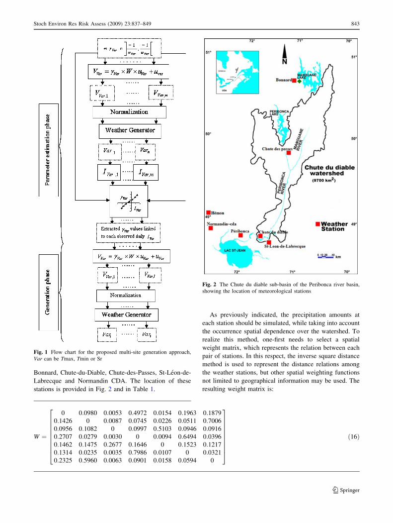
Figure 1 recapitulates the proposed multi-site generation

approach of daily temperature and solar radiation data. The

parameter estimation and the generation phases are pre-

sented for a given month. Var can be Tmax, Tmin or Sr. m

is the total number of cTmax, cTmin or cSr values taken from

their range, and l is the total number of days in a given

month. However, because solar radiation data are not

available for the used watershed, the multi-site model is

used only for maximum and minimum temperature. The

results presented are for a 50-year simulation period.

5 Results and discussion

5.1 Results of spatial intermittence approach

The multi-site generation approach of daily precipitation

data (Khalili et al. 2007) was tested with data from the

Chute du Diable sub-basin of the Peribonca River Basin

(Fig. 2). This region, which is characterized by a wet cli-

mate, relatively cool summers and snow precipitations

from November to April, is also used in this paper. Seven

stations in this watershed are selected: Peribonca, Hemon,


123

Bonnard, Chute-du-Diable, Chute-des-Passes, St-Leon-de-

Labrecque and Normandin CDA. The location of these

stations is provided in Fig. 2 and in Table 1.

As previously indicated, the precipitation amounts at

each station should be simulated, while taking into account

the occurrence spatial dependence over the watershed. To

realize this method, one-first needs to select a spatial

weight matrix, which represents the relation between each

pair of stations. In this respect, the inverse square distance

method is used to represent the distance relations among

the weather stations, but other spatial weighting functions

not limited to geographical information may be used. The

resulting weight matrix is:

Fig. 1 Flow chart for the proposed multi-site generation approach,

Var can be Tmax, Tmin or Sr

Fig. 2 The Chute du diable sub-basin of the Peribonca river basin,

showing the location of meteorological stations

W ¼

0 0:0980 0:0053 0:4972 0:0154 0:1963 0:1879

0:1426 0 0:0087 0:0745 0:0226 0:0511 0:7006

0:0956 0:1082 0 0:0997 0:5103 0:0946 0:0916

0:2707 0:0279 0:0030 0 0:0094 0:6494 0:0396

0:1462 0:1475 0:2677 0:1646 0 0:1523 0:1217

0:1314 0:0235 0:0035 0:7986 0:0107 0 0:0321

0:2325 0:5960 0:0063 0:0901 0:0158 0:0594 0

2

666666664

3

777777775

ð16Þ


123

The first row contains the spatial weights between the

Peribonca station and the other stations in the order given

above. The second row presents the spatial weights between

the Hemon station and the remaining stations, and so on.

Note that the spatial weight between each station and itself

is 0 by convention, and that the matrix is row-standardized.

Using the spatial dependence indicator (SDI) discussed

earlier, the spatial dependence of precipitation occurrences

was computed using the shared period for all stations,

which is 14 years starting from 1963 to 1976. Relation-

ships are then obtained between the mean of precipitation

amounts and the SDI values for each station and month.

Figure 3 shows an example of such a relationship obtained

for the Peribonca station in September. An exponential

regression fit is used to evaluate the mean of precipitation

amounts according to the spatial dependence of occurrence

values because it gives a best fit to the scatter plot.

As was introduced by Wilks (1998), the statistic ‘‘con-

tinuity ratio’’ is used to test the accuracy of the spatial

intermittence in the synthetic precipitation time series. This

statistic is computed for each pair of station (i,j), and is the

ratio of the mean of the nonzero precipitation amounts at

station i when station j is dry, to the mean of the nonzero

precipitation amounts at station i when station j is wet, such

that:

Continuity ratio ¼ E rt ið Þjrt ið Þ[ 0; rt jð Þ ¼ 0½ �E rt ið Þjrt ið Þ[ 0; rt jð Þ[ 0½ � ð17Þ

Figure 4a and b illustrate the spatial intermittence

results using the simple exponential function (a) and the

spatial exponential functions (b) to fit the precipitation

amounts. The use of the spatial exponential functions

greatly improves the results, and confirms the dependence

of the precipitation means at a given station on the

occurrence states at the set of stations. Each point in this

graph represents the continuity ratio for each pair of

stations and month. 504 points are therefore plotted in this

graph. The departure from the 45-degree reference line can

be attributed to the scatter plot obtained in certain

relationships between the mean of precipitation amounts

and the SDI values of the occurrences due to sampling

variations related to the small sample size (14 years).

5.2 Results of multi-site generation approach of daily

temperature data

As was the case for the precipitation processes (Khalili

et al. 2007), the multi-site generation approach of daily

temperature data was achieved using different weight

matrices. In a first step, the results for the row-standardized

weight matrix using the inverse square distance method,

presented above, are reported.

Using this weight matrix, the variation range of the

moving average coefficients cTmax and cTmin is ]-1;1.3254[,

according to the extreme eigenvalues of this matrix.

Therefore, taking values from this range, the synthetic

temperature data exhibit spatial autocorrelations ITmax and

Table 1 Location and recorded

years of the used stationsStations Latitude Longitude Elevation (m) Recorded years

Peribonca 48�450420 0N 72�010240 0W 107 1951–2002

Hemon 49�030480 0N 72�350350 0W 206 1963–2002

Chute-du-Diable 48�450000 0N 71�420000 0W 174 1951–1976

St-Leon de Labrecque 48�400260 0N 71�310330 0W 131 1963–1997

Normandin CDA 48�510000 0N 72�320000 0W 137 1936–1992

Chute-des-Passes 49�500250 0N 71�100060 0W 398 1960–1976

Bonnard 50�440000 0N 71�020000 0W 506 1961–2000

Nitchequon 53�120N 70�540W – 1960–1979

Shefferville 54�480N 66�490W – 1960–1979

Peribonca station

0

2

4

6

8

10

0 0.2 0.4 0.6 0.8 1 1.2

SDI of occurrences over the watershed

Mea

n o

f p

reci

pit

atio

n a

mo

un

ts (

mm

)

Fig. 3 Relationship between the mean of precipitation amounts (mm)

of Peribonca station and the spatial dependence values of occurrences

over the watershed in September


123

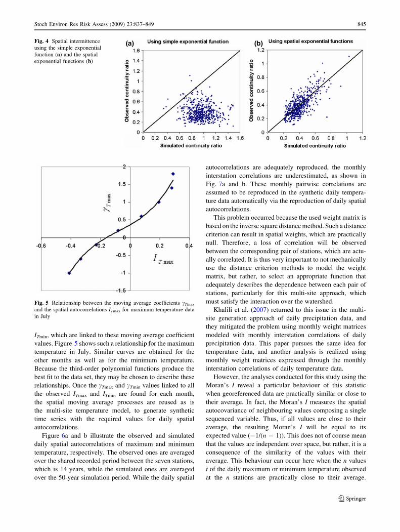
ITmin, which are linked to these moving average coefficient

values. Figure 5 shows such a relationship for the maximum

temperature in July. Similar curves are obtained for the

other months as well as for the minimum temperature.

Because the third-order polynomial functions produce the

best fit to the data set, they may be chosen to describe these

relationships. Once the cTmax and cTmin values linked to all

the observed ITmax and ITmin are found for each month,

the spatial moving average processes are reused as is

the multi-site temperature model, to generate synthetic

time series with the required values for daily spatial

autocorrelations.

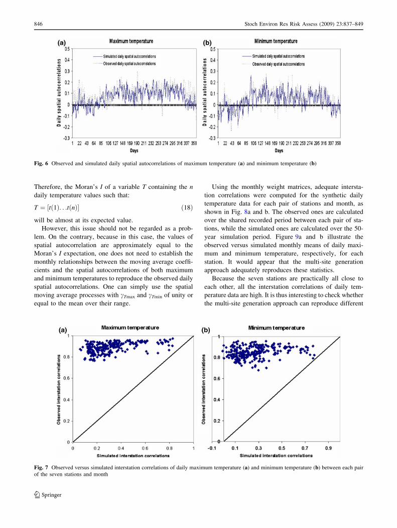
Figure 6a and b illustrate the observed and simulated

daily spatial autocorrelations of maximum and minimum

temperature, respectively. The observed ones are averaged

over the shared recorded period between the seven stations,

which is 14 years, while the simulated ones are averaged

over the 50-year simulation period. While the daily spatial

autocorrelations are adequately reproduced, the monthly

interstation correlations are underestimated, as shown in

Fig. 7a and b. These monthly pairwise correlations are

assumed to be reproduced in the synthetic daily tempera-

ture data automatically via the reproduction of daily spatial

autocorrelations.

This problem occurred because the used weight matrix is

based on the inverse square distance method. Such a distance

criterion can result in spatial weights, which are practically

null. Therefore, a loss of correlation will be observed

between the corresponding pair of stations, which are actu-

ally correlated. It is thus very important to not mechanically

use the distance criterion methods to model the weight

matrix, but rather, to select an appropriate function that

adequately describes the dependence between each pair of

stations, particularly for this multi-site approach, which

must satisfy the interaction over the watershed.

Khalili et al. (2007) returned to this issue in the multi-

site generation approach of daily precipitation data, and

they mitigated the problem using monthly weight matrices

modeled with monthly interstation correlations of daily

precipitation data. This paper pursues the same idea for

temperature data, and another analysis is realized using

monthly weight matrices expressed through the monthly

interstation correlations of daily temperature data.

However, the analyses conducted for this study using the

Moran’s I reveal a particular behaviour of this statistic

when georeferenced data are practically similar or close to

their average. In fact, the Moran’s I measures the spatial

autocovariance of neighbouring values composing a single

sequenced variable. Thus, if all values are close to their

average, the resulting Moran’s I will be equal to its

expected value (-1/(n - 1)). This does not of course mean

that the values are independent over space, but rather, it is a

consequence of the similarity of the values with their

average. This behaviour can occur here when the n values

t of the daily maximum or minimum temperature observed

at the n stations are practically close to their average.

Fig. 4 Spatial intermittence

using the simple exponential

function (a) and the spatial

exponential functions (b)

Fig. 5 Relationship between the moving average coefficients cTmax

and the spatial autocorrelations ITmax for maximum temperature data

in July


123

Therefore, the Moran’s I of a variable T containing the n

daily temperature values such that:

T ¼ ½tð1Þ. . .tðnÞ� ð18Þ

will be almost at its expected value.

However, this issue should not be regarded as a prob-

lem. On the contrary, because in this case, the values of

spatial autocorrelation are approximately equal to the

Moran’s I expectation, one does not need to establish the

monthly relationships between the moving average coeffi-

cients and the spatial autocorrelations of both maximum

and minimum temperatures to reproduce the observed daily

spatial autocorrelations. One can simply use the spatial

moving average processes with cTmax and cTmin of unity or

equal to the mean over their range.

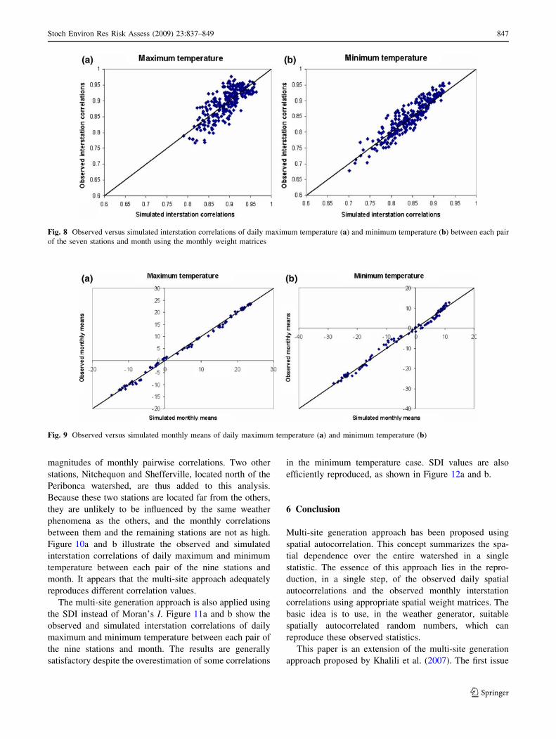
Using the monthly weight matrices, adequate intersta-

tion correlations were computed for the synthetic daily

temperature data for each pair of stations and month, as

shown in Fig. 8a and b. The observed ones are calculated

over the shared recorded period between each pair of sta-

tions, while the simulated ones are calculated over the 50-

year simulation period. Figure 9a and b illustrate the

observed versus simulated monthly means of daily maxi-

mum and minimum temperature, respectively, for each

station. It would appear that the multi-site generation

approach adequately reproduces these statistics.

Because the seven stations are practically all close to

each other, all the interstation correlations of daily tem-

perature data are high. It is thus interesting to check whether

the multi-site generation approach can reproduce different

Fig. 6 Observed and simulated daily spatial autocorrelations of maximum temperature (a) and minimum temperature (b)

Fig. 7 Observed versus simulated interstation correlations of daily maximum temperature (a) and minimum temperature (b) between each pair

of the seven stations and month


123

magnitudes of monthly pairwise correlations. Two other

stations, Nitchequon and Shefferville, located north of the

Peribonca watershed, are thus added to this analysis.

Because these two stations are located far from the others,

they are unlikely to be influenced by the same weather

phenomena as the others, and the monthly correlations

between them and the remaining stations are not as high.

Figure 10a and b illustrate the observed and simulated

interstation correlations of daily maximum and minimum

temperature between each pair of the nine stations and

month. It appears that the multi-site approach adequately

reproduces different correlation values.

The multi-site generation approach is also applied using

the SDI instead of Moran’s I. Figure 11a and b show the

observed and simulated interstation correlations of daily

maximum and minimum temperature between each pair of

the nine stations and month. The results are generally

satisfactory despite the overestimation of some correlations

in the minimum temperature case. SDI values are also

efficiently reproduced, as shown in Figure 12a and b.

6 Conclusion

Multi-site generation approach has been proposed using

spatial autocorrelation. This concept summarizes the spa-

tial dependence over the entire watershed in a single

statistic. The essence of this approach lies in the repro-

duction, in a single step, of the observed daily spatial

autocorrelations and the observed monthly interstation

correlations using appropriate spatial weight matrices. The

basic idea is to use, in the weather generator, suitable

spatially autocorrelated random numbers, which can

reproduce these observed statistics.

This paper is an extension of the multi-site generation

approach proposed by Khalili et al. (2007). The first issue


of the seven stations and month using the monthly weight matrices

Fig. 9 Observed versus simulated monthly means of daily maximum temperature (a) and minimum temperature (b)


123

was the improvement of the synthetic spatial intermittence.

The feasible solution presented here involves the approxi-

mation of the mean of precipitation amounts used in the

simple exponential function by a regression function of the

occurrence spatial dependence at the set of weather sta-

tions. Such a method was proposed because the mean of


of the nine stations and month using the monthly weight matrices


of the nine stations and month using the monthly weight matrices and SDI

Fig. 12 Observed and simulated daily spatial dependence of maximum temperature (a) and minimum temperature (b) using the monthly weight

matrices and SDI


123

precipitation amounts at a given station is not a free

parameter, but rather, depends on the occurrence states

over the watershed. Therefore, monthly spatial exponential

functions were established for each station. This approach

greatly improves the reproduction of synthetic spatial

intermittence.

A multi-site generation approach of daily maximum

temperature, minimum temperature and solar radiation data

was also presented in this paper. This approach adopted the

weakly stationary generating process used in the Richard-

son weather generator, with no modifications made to the

model, but only random numbers have to be spatially

autocorrelated. Spatial moving average processes were

used to generate the spatially autocorrelated random

numbers that can reproduce the observed daily spatial

autocorrelations in the synthetic time series. Because of a

lack of solar radiation data, the multi-site weakly stationary

generating process was only tested for maximum and

minimum temperature data. This approach has been shown

to perform well in the generation of these data. Sufficiently

accurate daily spatial autocorrelations and monthly inter-

station correlations were obtained in the synthetic time

series.

Finally, results presented in this paper show the effi-

ciency of the developed multi-site weather generator and

its ease of implementation. The use of multi-site generated

weather data is important to account for weather spatial

dependence, which has a significant effect on various

meteorology dependent projects, such as hydrological

modelling and other environmental research.

Acknowledgments This research was supported by the Natural

Science and Engineering Research Council of Canada, Hydro-Quebec

and the Ouranos Consortium on climate change through a collabo-

rative research and development grant. Their support is gratefully

acknowledged.

References

Anselin L (1980) Estimation methods for spatial autoregressive

structures, No. 8. Regional science dissertation and monograph

series, Cornell University, Ithaca

Bardossy A, Plate EJ (1992) Space-time model for daily rainfall using

atmospheric circulation patterns. Water Resour Res 28:1247–

1259

Bellone E, Hughes JP, Guttorp P (2000) A hidden Markov model for

downscaling synoptic atmospheric patterns to precipitation

amounts. Clim Res 15:1–12

Bogardi I, Matyasovszky I, Bardossy A, Duckstein L (1993)

Application of a space-time stochastic model for daily precip-

itation using atmospheric circulation patterns. J Geophys Res

98:16653–16667

Brandsma T, Buishand TA (1997) Rainfall generator for the Rhine

basin; single-site generation of weather variables by nearest-

neighbour resampling. KNMI-publicatie 186–1, KNMI, De Bilt,

47 pp

Brissette F, Khalili M, Leconte R (2007) Efficient stochastic

generation of multi-site synthetic precipitation data. J Hydrol

345(3–4):121–133

Buishand TA, Brandsma T (2001) Multisite simulation of daily

precipitation and temperature in the Rhine basin by nearest-

neighbour resampling. Water Resour Res 37(11):2761–2776

Cliff AD, Ord JK (1981) Spatial processes: models and applications.

Pion, London

Cressie NAC (1993) Statistics for spatial data. Wiley series in

probability and mathematical statistics. Wiley, London, 900 pp

Griffith DA (2003) Spatial autocorrelation and spatial filtering:

gaining understanding through theory and scientific visualiza-

tion. In: Advances in spatial science. Springer, Heidelberg,

247 pp

Hughes JP, Guttorp P (1994a) A class of stochastic models for

relating synoptic atmospheric patterns to regional hydrologic

phenomena. Water Resour Res 30:1535–1546

Hughes JP, Guttorp P (1994b) Incorporating spatial dependence and

atmospheric data in a model of precipitation. J Appl Meteorol

33:1503–1515

Hughes JP, Guttorp P, Charles S (1999) A nonhomogeneous hidden

Markov model for precipitation occurrence. Appl Stat 48:15–30

Khalili M, Leconte R, Brissette F (2007) Stochastic multi-site

generation of daily precipitation data using spatial autocorrela-

tion. J Hydrometeorol 8(3):396–412

Matalas NC (1967) Mathematical assessment of synthetic hydrology.

Water Resour Res 3(4):937–945

Moran PAP (1950) Notes on continuous stochastic phenomena.

Biometrika 37:17–23

Murdoch JC, Rahmatian M, Thayer MA (1993) A spatially autore-

gressive median voter model of recreation expenditures. Public

Finan Q 21:334–350

Odland J (1988) Spatial autocorrelation. Sage Publications, Newbury

Park, p 87

Richardson CW (1981) Stochastic simulation of daily precipitation,

temperature, and solar radiation. Water Resour Res 17(1):182–

190

Richardson CW, Wright DA (1984) WGEN: a model for generating

daily weather variables. US Department of Agriculture, Agri-

cultural Research Service, ARS-8, 83 pp

Semenov MA, Barrow EM (1997) Use of a stochastic weather

generator in the development of climate change scenarios. Clim

Change 22:67–84

Tobler W (1970) A computer movie simulating urban growth in the

Detroit region. Econ Geogr 46:234–240

Tae-woong K, Hosung A, Gunhui Ch (2007) Stochastic multi-site

generation of daily rainfall occurrence in south Florida. J Stoch

Environ Res Risk Assess. doi:10.1007/s00477-007-0180-8

Ullah M, Giles DEA (1991) Handbook of applied economic statistics.

Marcel Dekker Inc., New York, pp 237–289

Wilks DS (1998) Multisite generalization of a daily stochastic

precipitation generation model. J Hydrol 210:178–191

Wilks DS (1999) Simultaneous stochastic simulation of daily

precipitation, temperature and solar radiation at multiple sites

in complex terrain. Agric For Meteorol 96:85–101


123

http://dx.doi.org/10.1007/s00477-007-0180-8

Khalili, M., Brissette, F., Leconte, R., 2009, Stochastic Multi-Site ...

Documents

Transcript of Khalili, M., Brissette, F., Leconte, R., 2009, Stochastic Multi-Site ...