Keyu Wu - University of Alberta

Machine Learning Approaches for Wireless Spectrum andEnergy Intelligence

by

Keyu Wu

A thesis submitted in partial fulfillment of the requirements for the degree of

Doctor of Philosophy

in

Communications

Department of Electrical and Computer Engineering

University of Alberta

c© Keyu Wu, 2018

Abstract

Cognitive radio and energy-harvesting technologies improve the efficiency of spectrum use

and energy use in communication networks. However, due to the randomness and dynamics

of spectral and energy resources, wireless nodes must intelligently adjust their operating

configurations (radio frequency and transmission power). With machine learning as primary

tools, this thesis addresses three spectrum and energy management problems.

First, we consider a single-channel energy-harvesting cognitive transmitter, which at-

tempts to maximize data throughput with harvested energy and dynamically available

channel. The transmitter needs to determine whether or not to perform spectrum sens-

ing and channel probing, and how much power for transmission, subject to energy status

and wireless channel state. The resulting control problem is addressed by a two-stage rein-

forcement learning algorithm, which finds the optimal policy from data samples when the

statistical distributions of harvested energy and channel fading are unknown.

Second, we consider energy-harvesting sensor, which strives to deliver packets with finite

battery capacity and random energy replenishment. A selective transmission strategy is

investigated, where low priority packets can be dropped to save energy for high priority

data packets. The optimal transmission policy, which determines whether or not a packet

should be transmitted, is derived via training an artificial neural network with data samples

of packet priorities, wireless channel gains, and harvested energy levels.

Third, we investigate cooperation among cognitive nodes for reliable spectrum sensing

given spectrum heterogeneity (i.e., spatial dependence of spectrum availability). Sensing

cooperation can mitigate it. However, the challenge is how to model and exploit spatial

correlations to fuse sensing data. To overcome this, spatial correlations among cognitive

nodes are modeled as a Markov random field; and given data observations, sensing coop-

eration is achieved by solving a maximum posterior probability estimator over the Markov

random field. Under this methodology, three cooperative sensing algorithms are designed

for centralized, cluster-based, and distributed cognitive radio networks. These algorithms

offer improved computational efficiency and reduced communication overhead.

ii

Preface

This thesis is an original work by Keyu Wu. Parts of the thesis have been published or

submitted to journals or conferences, which are indicated below.

Partial work of Chapter 3 is represented at IEEE ICC 2017 as “K. Wu, H. Jiang and C.

Tellambura, ‘Sensing, Probing, and Transmitting strategy for Energy Harvesting Cognitive

Radio,’ 2017 IEEE ICC, Paris, 2017”. The full length version is submitted to IEEE Trans-

action of Vehicular Technology in May 2018 as “K. Wu and H. Jiang, and C. Tellambura,

‘Sensing, Probing and Transmitting Policy for Energy Harvesting Cognitive Radio with

two-stage After-state Reinforcement Learning’ ”.

Partial work of Chapter 4 is represented at IEEE ICC 2017 as “K.Wu, C. Tellambura and

H. Jiang, ‘Optimal Transmission Policy in Energy Harvesting Wireless Communications: A

Learning Approach,’ 2017 IEEE ICC, Paris, 2017”. The full length version is submitted

to IEEE Internet of Things Journal in July 2018 as “K. Wu, F. Li, C. Tellambura, and H.

Jiang, ‘Optimal Selective Transmission Policy for Energy-Harvesting Wireless Sensors via

Monotone Neural Networks’ ”.

A tutorial version of Chapter 5 is published as “K. Wu, M. Tang, C. Tellambura and D.

Ma, ‘Cooperative Spectrum Sensing as Image Segmentation: A New Data Fusion Scheme,’

in IEEE Communications Magazine, vol. 56, no. 4, pp. 142-148, April 2018”.

iii

Acknowledgements

I sincerely appreciate my supervisors, Dr. Chintha Tellambura and Dr. Hai Jiang, for

their guidance, encouragement, advice and support. In the course of this thesis research,

I had been greatly benefited from their profound knowledge and expertise. Their research

attitude and standard have set me a valuable example, and will continue influencing me in

my future career.

I would like to thank my thesis examining committee members Dr. Yindi Jing, Dr.

Ehab Elmallah, and Dr. Dongmei Zhao for their time and efforts in reviewing my thesis

and providing me valuable comments. Their feedbacks helped me to improve the quality of

the thesis.

I also like to thank all professors who delivered courses during my study, which makes

me prepared for the research. Especially, I would like to thank Dr. Richard Sutton for

his excellent lecture on reinforcement learning, which continuously inspired throughout the

research.

Especial gratitude also goes to present and former colleagues of iCore Wireless Commu-

nications Lab W5-070 and Advanced Wireless Communications and Signal Processing Lab

W5-077 for their continual help and companion.

Most importantly, I am very thankful to my family, including my parents, my brother,

my parents-in-law and especially my wife, Mrs. Tiantian Huang. It is their understanding

and unconditional support that help me to get through all difficulties in the four years’

path.

Last but not least, I would like to thank all funders throughout my PhD study, including

the CSC Scholarship, Alberta Innovates Technology Futures (AITF) Top-up Scholarship,

FGSR Travel Awards and IEEE ICC Student Travel Grants. Without their finding support,

I could not have completed the PhD study.

iv

Contents

1 Introduction 1

1.1 Communications with Recycled Spectrum and Energy . . . . . . . . . . . . 1

1.1.1 The next generation wireless systems . . . . . . . . . . . . . . . . . . 1

1.1.2 Spectrum and energy considerations . . . . . . . . . . . . . . . . . . 1

1.1.3 Cognitive radio: recycle spectrum from primary users . . . . . . . . 2

1.1.4 Energy-harvesting: recycle energy from environments . . . . . . . . 3

1.2 Management of Spectrum Holes . . . . . . . . . . . . . . . . . . . . . . . . . 4

1.2.1 Spectrum sensing and access . . . . . . . . . . . . . . . . . . . . . . 4

1.2.2 Cooperative spectrum sensing . . . . . . . . . . . . . . . . . . . . . . 5

1.2.3 Cooperative transmission . . . . . . . . . . . . . . . . . . . . . . . . 5

1.3 Management of Harvested Energy . . . . . . . . . . . . . . . . . . . . . . . 6

1.3.1 Handling dynamic battery status . . . . . . . . . . . . . . . . . . . . 6

1.3.2 Incorporating data-centric consideration . . . . . . . . . . . . . . . . 6

1.3.3 Simultaneous information and power transfer . . . . . . . . . . . . . 7

1.4 Thesis Motivation and Contributions . . . . . . . . . . . . . . . . . . . . . . 7

1.4.1 Brief introduction of machine learning . . . . . . . . . . . . . . . . . 7

1.4.2 Machine learning approaches for spectrum and energy intelligence . 9

1.5 Thesis Outlines . . . . . . . . . . . . . . . . . . . . . . . . . . . . . . . . . . 11

2 Background 12

2.1 MDP and After-state . . . . . . . . . . . . . . . . . . . . . . . . . . . . . . . 12

2.1.1 Problem setting of MDP . . . . . . . . . . . . . . . . . . . . . . . . . 12

2.1.2 Standard results for MDP control . . . . . . . . . . . . . . . . . . . . 13

2.1.3 MDP control based on after-states . . . . . . . . . . . . . . . . . . . 13

2.2 Artificial Neural Network . . . . . . . . . . . . . . . . . . . . . . . . . . . . 15

2.2.1 Neural network as a function . . . . . . . . . . . . . . . . . . . . . . 16

v

2.2.2 Train neural networks with labeled data . . . . . . . . . . . . . . . . 17

2.3 Markov Random Field . . . . . . . . . . . . . . . . . . . . . . . . . . . . . . 18

2.4 Summary . . . . . . . . . . . . . . . . . . . . . . . . . . . . . . . . . . . . . 20

3 Sensing-Probing-Transmission Control for Energy-Harvesting Cognitive

Radio 21

3.1 Introduction . . . . . . . . . . . . . . . . . . . . . . . . . . . . . . . . . . . . 21

3.1.1 Related works . . . . . . . . . . . . . . . . . . . . . . . . . . . . . . . 22

3.1.2 Problem statement and contributions . . . . . . . . . . . . . . . . . 24

3.2 System Model . . . . . . . . . . . . . . . . . . . . . . . . . . . . . . . . . . . 25

3.3 Two-stage MDP Formulation . . . . . . . . . . . . . . . . . . . . . . . . . . 28

3.3.1 Finite step machine for MAC protocol . . . . . . . . . . . . . . . . . 28

3.3.2 Two-stage MDP . . . . . . . . . . . . . . . . . . . . . . . . . . . . . 30

3.3.3 Optimal control via state value function V ∗ . . . . . . . . . . . . . . 33

3.4 After-state Reformulation . . . . . . . . . . . . . . . . . . . . . . . . . . . . 34

3.4.1 Structure of the MDP . . . . . . . . . . . . . . . . . . . . . . . . . . 34

3.4.2 Introducing after-state based control . . . . . . . . . . . . . . . . . . 35

3.4.3 Establishing after-state based control . . . . . . . . . . . . . . . . . . 36

3.5 Reinforcement Learning Algorithm . . . . . . . . . . . . . . . . . . . . . . . 38

3.5.1 After-state space discretization . . . . . . . . . . . . . . . . . . . . . 38

3.5.2 Learn optimal policy with data samples . . . . . . . . . . . . . . . . 39

3.5.3 Theoretical soundness and performance bounds . . . . . . . . . . . . 41

3.5.4 Simultaneous sampling, learning and control . . . . . . . . . . . . . 43

3.6 Simulation Results . . . . . . . . . . . . . . . . . . . . . . . . . . . . . . . . 47

3.6.1 Simulation setup . . . . . . . . . . . . . . . . . . . . . . . . . . . . . 47

3.6.2 Characteristics of online learning algorithm . . . . . . . . . . . . . . 48

3.6.3 Myopic versus holistic . . . . . . . . . . . . . . . . . . . . . . . . . . 49

3.7 Summary . . . . . . . . . . . . . . . . . . . . . . . . . . . . . . . . . . . . . 51

3.8 Appendix . . . . . . . . . . . . . . . . . . . . . . . . . . . . . . . . . . . . . 52

3.8.1 Proof of Theorem 3.1 . . . . . . . . . . . . . . . . . . . . . . . . . . 52

3.8.2 Proof of Theorem 3.2 . . . . . . . . . . . . . . . . . . . . . . . . . . 53

3.8.3 Proof of Theorem 3.3 . . . . . . . . . . . . . . . . . . . . . . . . . . 54

4 Optimal Selective Transmission for Energy-Harvesting Wireless Sensors 59

4.1 Introduction . . . . . . . . . . . . . . . . . . . . . . . . . . . . . . . . . . . . 59

vi

4.1.1 Motivation, problem statement and contributions . . . . . . . . . . . 61

4.2 System Model and Problem Formulation . . . . . . . . . . . . . . . . . . . . 62

4.2.1 Operation cycles . . . . . . . . . . . . . . . . . . . . . . . . . . . . . 62

4.2.2 States and actions . . . . . . . . . . . . . . . . . . . . . . . . . . . . 63

4.2.3 State dynamics . . . . . . . . . . . . . . . . . . . . . . . . . . . . . . 64

4.2.4 Rewards . . . . . . . . . . . . . . . . . . . . . . . . . . . . . . . . . . 65

4.2.5 Problem formulation . . . . . . . . . . . . . . . . . . . . . . . . . . . 65

4.3 Optimal Selective Transmission Policy . . . . . . . . . . . . . . . . . . . . . 66

4.3.1 Standard results from MDP theory . . . . . . . . . . . . . . . . . . . 66

4.3.2 Reformulation based on after-state value function . . . . . . . . . . . 66

4.3.3 Properties of J∗ and π∗ . . . . . . . . . . . . . . . . . . . . . . . . . 68

4.3.4 An example of J∗ and π∗ . . . . . . . . . . . . . . . . . . . . . . . . 69

4.4 Neural Network for Optimal Control . . . . . . . . . . . . . . . . . . . . . . 70

4.4.1 Monotone neural network approximation . . . . . . . . . . . . . . . 71

4.4.2 Fitted value iteration to train MNN . . . . . . . . . . . . . . . . . . 73

4.4.3 Apply learned MNN for transmission control . . . . . . . . . . . . . 77

4.5 Numerical Simulation . . . . . . . . . . . . . . . . . . . . . . . . . . . . . . 78


4.5.2 Sample efficiency for learning π∗ . . . . . . . . . . . . . . . . . . . . 79

4.5.3 Achieved performance of learned policy . . . . . . . . . . . . . . . . 82

4.6 Summary . . . . . . . . . . . . . . . . . . . . . . . . . . . . . . . . . . . . . 83

4.7 Appendix . . . . . . . . . . . . . . . . . . . . . . . . . . . . . . . . . . . . . 83

4.7.1 Proof of Lemma 4.1 . . . . . . . . . . . . . . . . . . . . . . . . . . . 83

4.7.2 Proof of Theorem 4.1 . . . . . . . . . . . . . . . . . . . . . . . . . . 84

4.7.3 Proof of Lemma 4.2 . . . . . . . . . . . . . . . . . . . . . . . . . . . 86

5 Cooperative Spectrum Sensing under Heterogeneous Spectrum Availabil-

ity 87

5.1 Introduction . . . . . . . . . . . . . . . . . . . . . . . . . . . . . . . . . . . . 87

5.1.1 Motivations . . . . . . . . . . . . . . . . . . . . . . . . . . . . . . . . 89

5.1.2 Contributions . . . . . . . . . . . . . . . . . . . . . . . . . . . . . . . 89

5.2 System Model . . . . . . . . . . . . . . . . . . . . . . . . . . . . . . . . . . . 91

5.2.1 Network setup . . . . . . . . . . . . . . . . . . . . . . . . . . . . . . 91

5.2.2 Signal model and data likelihood functions . . . . . . . . . . . . . . 91

vii

5.3 CSS with MAP-MRF Formulation . . . . . . . . . . . . . . . . . . . . . . . 93

5.3.1 Define SU-graph and MRF . . . . . . . . . . . . . . . . . . . . . . . 94

5.3.2 Fuse data over MRF . . . . . . . . . . . . . . . . . . . . . . . . . . . 94

5.4 GC-CSS for Centralized Secondary Networks . . . . . . . . . . . . . . . . . 96

5.4.1 BF-graph and min-cut . . . . . . . . . . . . . . . . . . . . . . . . . . 97

5.4.2 MAP-MRF = min-cut . . . . . . . . . . . . . . . . . . . . . . . . . . 99

5.5 DD-CSS for Cluster-based Secondary Networks . . . . . . . . . . . . . . . . 100

5.5.1 Divide SU-graph into subgraphs . . . . . . . . . . . . . . . . . . . . 101

5.5.2 DD-CSS: inter-cluster message passing algorithm . . . . . . . . . . . 103

5.6 DD1-CSS for Distributed Secondary Networks . . . . . . . . . . . . . . . . . 112

5.6.1 Two-hop message-passing . . . . . . . . . . . . . . . . . . . . . . . . 112

5.6.2 Compared with belief propagation algorithms . . . . . . . . . . . . . 114

5.7 Numerical Simulations . . . . . . . . . . . . . . . . . . . . . . . . . . . . . . 115


5.7.2 Choosing hyperparameter β . . . . . . . . . . . . . . . . . . . . . . . 117

5.7.3 Performance gain and loss of MAP-MRF . . . . . . . . . . . . . . . 117

5.7.4 Maximization v.s. Marginalization . . . . . . . . . . . . . . . . . . . 119

5.7.5 Computation complexity . . . . . . . . . . . . . . . . . . . . . . . . . 120

5.8 Summary . . . . . . . . . . . . . . . . . . . . . . . . . . . . . . . . . . . . . 121

6 Conclusions and Future Research 122

6.1 Conclusions . . . . . . . . . . . . . . . . . . . . . . . . . . . . . . . . . . . . 122

6.2 Future Research . . . . . . . . . . . . . . . . . . . . . . . . . . . . . . . . . 123

6.2.1 Optimal sensing-probing policy without primary user model . . . . . 123

6.2.2 Multi-link selective transmission for energy-harvesting sensors . . . . 123

6.2.3 Learn MRF model from data . . . . . . . . . . . . . . . . . . . . . . 123

Bibliography 124

viii

List of Tables

2.1 Pairwise potential function φ(xi, xj) . . . . . . . . . . . . . . . . . . . . . . 20

3.1 Structured state transition model . . . . . . . . . . . . . . . . . . . . . . . . 35

ix

List of Figures

2.1 The problem setting of MDP . . . . . . . . . . . . . . . . . . . . . . . . . . 12

2.2 Paper-and-pencil game Tic-Tac-Toe . . . . . . . . . . . . . . . . . . . . . . 14

2.3 From state-action pairs to after-states . . . . . . . . . . . . . . . . . . . . . 15

2.4 A three-layer neural network . . . . . . . . . . . . . . . . . . . . . . . . . . 16

2.5 Sigmoid function . . . . . . . . . . . . . . . . . . . . . . . . . . . . . . . . . 17

2.6 An binary image segmentation example; northwest: original image; north-

east: image contaminated by salt-and-pepper noise; southwest: thresholding

segmentation; southeast: segmentation incorporating MRF. . . . . . . . . . 19

2.7 Graph G for a nine-pixel image . . . . . . . . . . . . . . . . . . . . . . . . . 19

3.1 The PU’s channel occupancy model . . . . . . . . . . . . . . . . . . . . . . 26

3.2 Time slot structure . . . . . . . . . . . . . . . . . . . . . . . . . . . . . . . . 27

3.3 FSM for MAC protocol . . . . . . . . . . . . . . . . . . . . . . . . . . . . . 30

3.4 Two-stage MDP . . . . . . . . . . . . . . . . . . . . . . . . . . . . . . . . . 30

3.5 Augmented MDP model with after-state . . . . . . . . . . . . . . . . . . . . 36

3.6 An example of after-state space discretization . . . . . . . . . . . . . . . . . 39

3.7 Learning curves under various exploration rates . . . . . . . . . . . . . . . . 48

3.8 Learning curves under various update sizes . . . . . . . . . . . . . . . . . . 49

3.9 Channel access probability under different µE . . . . . . . . . . . . . . . . . 50

3.10 Data rates for different µE . . . . . . . . . . . . . . . . . . . . . . . . . . . . 51

4.1 Cycle structure . . . . . . . . . . . . . . . . . . . . . . . . . . . . . . . . . . 63

4.2 Examples for after-state value function and optimal policy . . . . . . . . . . 69

4.3 Monotone neural network . . . . . . . . . . . . . . . . . . . . . . . . . . . . 72

4.4 Illustration of FMNN with |F| = 500 . . . . . . . . . . . . . . . . . . . . . . 75

4.5 Learning curve . . . . . . . . . . . . . . . . . . . . . . . . . . . . . . . . . . 80

4.6 Learned value functions . . . . . . . . . . . . . . . . . . . . . . . . . . . . . 81

4.7 Achieved performance under different channel conditions . . . . . . . . . . . 82

x

5.1 Network setup . . . . . . . . . . . . . . . . . . . . . . . . . . . . . . . . . . 91

5.2 An example of SU-graph . . . . . . . . . . . . . . . . . . . . . . . . . . . . . 97

5.3 BF-graph and graph cuts . . . . . . . . . . . . . . . . . . . . . . . . . . . . 98

5.4 Cluster-based secondary network . . . . . . . . . . . . . . . . . . . . . . . . 101

5.5 Subgraphs overlapped at gate-SUs . . . . . . . . . . . . . . . . . . . . . . . 103

5.6 Solve master problem via iteratively solving slave problems . . . . . . . . . 107

5.7 Communicating SUs of SU3 for DD1-CSS . . . . . . . . . . . . . . . . . . . 114

5.8 Pe for GC-CSS under different β and SU densities . . . . . . . . . . . . . . 117

5.9 Pe for Ind-SS, GC-CSS, localization and Dist-GC-CSS algorithms . . . . . . 118

5.10 ROC for sensing algorithms . . . . . . . . . . . . . . . . . . . . . . . . . . . 119

5.11 CPU time per unit under different number of SUs . . . . . . . . . . . . . . 121

xi

List of Symbols

Symbols in Chapter 3

a action of an MDP

b battery level

Bmax battery capacity

C PU channel status

d endogenous component of a state

eH harvested energy

eS energy required for sensing

eP energy required for probing

eT energy required for transmitting

FB feedback indicator form SU receiver

fE probability density function of harvested energy

fH probability density function of channel gain

h wireless channel gain

J∗ after-state value function

p belief of channel availability

r reward function

s state

V ∗ state value function

x exogenous component of a state

π∗ optimal policy

β after-state

Θ spectrum sensing result

xii


a action of an MDP

b battery level

c total energy consumption for standing by, data reception and channel estimation

d data importance value

e harvested energy

fB transition probability of battery level given an after-state

fD probability density function of data importance values

fE probability density function of harvested energy

fH probability density function of required energy for tranmission

h required energy for transmission

J∗ after-state value function

p after-state

r reward function

s state

V ∗ state value function

z channel power gain

θ parameter vector of MNN


c edge cost of a BF graph

di distance from the ith SU to the PU

fY |X data likelihood function

K a graph cut

x all SUs’ spectrum statuses

xi the ith SU’s spectrum status

y all SUs’ sensing observation

yi the ith SU’s sensing observation

E the edge set of a graph

G a graph

V the node set of a graph

xiii

α channel propagation factor

ψi complex channel gain of a fading channel

φ potential function between a pair of neighboring SUs

ΦX MRF over SU spectrum statuses

λ Lagrange multiplier

xiv

Glossary of Terms

Acronyms Definition

ANN artificial neural network

BP belief propagation

CSS cooperative spectrum sensing

CSI channel status information

MAC medium access control

MAP maximum a posterior

MDP Markov decision process

MNN monotone neural network

MRF Markov random field

PDF probability density function

PrR protection range

PU primary user

SU secondary user

xv

Chapter 1

Introduction

1.1 Communications with Recycled Spectrum and Energy

1.1.1 The next generation wireless systems

The next generation (5G) wireless communications system will begin their deploy-

ment in 2020. 5G is designed to support various applications subject to stringent

technical requirements [1]. For example, to support data-intensive applications, in-

cluding steaming video, online gaming, and virtual reality, 5G promises 1000 times

higher data rate (1 to 10 Gb per second) compared with current 4G systems. Be-

sides human-centric applications, machine-type communications, including Internet

of Things and self-driving cars, are also important application scenarios of 5G. Since

machine-type communications may involve a massive number of devices, such as sen-

sors or actors, it is expected that 5G should be able to support 1 million connections

per square km. In addition, for securing latency-critical applications (such as car-

to-car communications or industrial control), 5G is required to provide 10 times less

latency (1 millisecond) than 4G.

1.1.2 Spectrum and energy considerations

1.1.2.1 Spectrum efficiency is a key

Radio spectrum is probably the most important resource for wireless communications.

However, wireless spectrum has almost been assigned to different wireless applications

(such as telecommunications, televisions, radio, radar, navigation, etc.) [2]. It is very

difficult and expensive to obtain additional spectrum bands for 5G use. For example,

a 70 MHz spectrum band (at 600 MHz) that was utilized for television broadcasting

1

has been reassigned for 5G use with 19.8 billion dollars cost in spectrum auction [3].

Although it is promising1 to obtain several new spectrum bands from mmWave range

(24-84 GHz), due to poor propagation characteristics, mmWave bands are mainly

exploited to meet extreme bandwidth requirements from local traffic “hot spots”

(such as stadiums or urban areas). Many 5G application scenarios, such as connecting

widely deployed devices, providing necessary capacity and supporting user mobility,

mainly rely on spectrum below 6 GHz [5]. In summary, the development of 5G is

constrained under spectrum crunch (especially sub 6 GHz), and therefore, improving

spectrum use efficiency is a key for the success of 5G.

1.1.2.2 Energy efficiency ensures affordability and sustainability

The efficient use of energy is another important design consideration of 5G for decreas-

ing costs and environmental impacts. Specifically, it is reported that “currently 3%

of the world-wide energy is consumed by the Information & Communications Tech-

nology infrastructure that causes about 2% of the world-wide CO2 emissions, which

is comparable to the world-wide CO2 emissions by airplanes or one quarter of the

world-wide CO2 emissions by cars” [6]. Under the dramatic increase of services and

data demands, if not carefully designed, 5G may further increase energy consumption

and carbon footprint. For example, it is expected that, without energy efficient plan

and management, communication industry may use as much as 51% of global elec-

tricity in 2030 under the current growth trend of devices, infrastructures and data

traffic [7]. Therefore, improving energy use efficiency is crucial for affordability and

sustainability of 5G.

1.1.3 Cognitive radio: recycle spectrum from primary users

Although an apparent spectrum scarcity is indicted in [2], deeper investigations reveal

encouraging results. Specifically, several field experiments suggest that, at given

time and location, large portion (between 80% and 90%) of the licensed spectrum is

idle [8]. The result is an underutilization of radio spectrum. These temporally unused

spectrum bands, a.k.a., spectrum holes, arise because most of primary (licensed) user

access is bursty.1 As an example, the Federal Communications Commission is working on allocating 5 licensed spectrum

bands (24.25-24.45, 24.75-25.25, 27.5-28.35, 37-38.6 and 38.6-40 GHz) for 5G applications [4].

2

Cognitive radio, proposed in [9], is a software-defined radio that has the ability

to perceive environments, adjust operating configuration and learn from experience.

These features make cognitive radio an ideal solution to recycle temporally available

spectrum holes from primary systems (radar, television systems, etc.), which is known

as dynamic spectrum access. Specifically, by sensing spectrum bands (i.e., channels),

cognitive/secondary nodes detect primary user activities, and access a channel if it is

not occupied. This dynamic access scheme would provide 5G an efficient and flexible

solution to further exploit underutilized spectrum and improve overall spectrum use

efficiency and communication capacity.

1.1.4 Energy-harvesting: recycle energy from environments

One of the energy consumption drivers of 5G will be the massive number of machine

type communication devices, such as wireless sensors (which are “eyes” and “ears”

for the Internet of Things and other applications). Although these devices generally

operate with low power, their massive population (expected to reach 21 billions in

2020) will make the total energy consumption non-negligible. Furthermore, compared

with the operation stage, production and deployment of these devices may cause the

same order (if not higher) energy consumption. Specifically, semiconductor devices

need highly complicated manufacturing process. Therefore, (unlike other electrical

machines, such as cars and refrigerators) for these high-tech devices, the energy con-

sumption in the production stage could be even higher than that of the operation

stage [10]. What’s worse, since in many application, these devices are deployed ex-

tensively in large areas for environment monitoring, replacing or recharging battery

may not be an option. Therefore, new devices have to be periodically redeployed to

compensate node losses due to drained batteries.

Energy-harvesting technology provides a solution to the aforementioned problems.

Energy-harvesting devices are able to recycle energy from ambient environments, such

as sunlight, indoor illumination, electromagnetic energy, etc [11]. The key compo-

nent of an energy-harvesting device is called an energy-harvesting transducer, which

can convert other types of physical quantities, such as pressure or brightness, into

electricity. As reported in [12], an energy harvester is capable to produce 140 mW

of power with small enough size for portable electronic devices (note that the trans-

3

mit power of a wireless sensor node generally varies from 100 µW to 100 mW [13]).

Hence, equipping low-power communication devices with energy harvester leads to

the self-sufficiency of energy [13], which could cut off the energy expenditure to power

these devices. Further, empowered with energy-harvesting, the life time of sensors is

not constrained by battery capacity, but reaches the limits of hardware [14], which

greatly reduces the energy cost for reproduction and redeployment.

1.2 Management of Spectrum Holes

The core idea of cognitive radio (dynamic spectrum access) is to access primary user

spectrum without causing interference. However, this goal is challenging due to the

dynamic activities of primary users, as the spectrum holes created by the inactivity

of primary users thus change over time and location. Therefore, the use of spectrum

holes by cognitive nodes must be managed carefully.

1.2.1 Spectrum sensing and access

Reliable spectrum sensing enables secondary nodes to correctly identify spectrum

holes while minimizing interference to primary users. For example, in IEEE standard

802.22, the mis-detection probability for detecting licensed television transmitters

should be not larger than 0.1 [15]. In addition, agility is also desired. Faster spectrum

sensing provides more transmission time over sensed spectrum holes, which increases

data throughput [16]. Various signal processing techniques have been considered [17]

for handling the reliability and agility trade-off.

In multi-channel systems, it is generally impractical to sense all channels simul-

taneously due to hardware limitations. When a cognitive node can only sense and

access one channel at a moment, the node needs to decide by what order the channels

should be scanned, and in addition, given a sensed spectrum hole, whether or not to

stop scanning and exploit the spectrum hole [18–20]. When primary activities have

temporal correlation [21,22], sensing observations can be used for predicting primary

activities (i.e., future channel status). In this case, spectrum sensing decision may

need to balance between the two goals: identifying idle channel for immediate use

and tracking primary activities to guide future decisions.

4

1.2.2 Cooperative spectrum sensing

Due to wireless propagation impairments such as shadowing and fading, spectrum

sensing by an individual node may not meet reliability requirements within an ac-

ceptable sensing time duration. Specifically, due to the shadowing effect caused by

objects obstructing, primary signal may be largely blocked at certain cognitive nodes.

In addition, when wireless channel (between a primary transmitter and a cognitive

node) undergoes deep fading, the received primary signal can be weak. Moreover,

when the coherence time is large, the fading may last for long time. All these factors

considerably increase required time to accumulate week signal for reliable detection.

Fortunately, the sensing reliability and agility can be improved by intelligently

fusing sensing observations from multiple, spatially-separate secondary nodes, which

is known as cooperative spectrum sensing (CSS) [23]. The fundamental reason is that

the simultaneous deep fading and shadowing of channels to multiple users is highly

unlikely. Various data fusion techniques have been considered [16, 24–26], which can

be roughly categorized as soft-combining schemes (combining raw received signals)

and hard-combining schemes (combining binary decisions).

1.2.3 Cooperative transmission

Cognitive radio networks can be benefited by relaying data with intermediate nodes,

known as cooperative transmission. First, for large networks, cognitive nodes at dif-

ferent locations may observe different spectrum holes. Two cognitive nodes cannot

establish direct communication link, if there is no common spectrum hole between

them. However, in the context of cooperative transmission, communication is possi-

ble whenever there exists a multi-hop-multi-channel path between two communicat-

ing nodes. This significantly reduces the likelihood of experiencing communication

breakdown due to “spectrum outage” [27]. In addition, with clever relay selection and

signal combining, a cognitive node is able to transmit with a lower power compared

with the direct-link case [28–30]. This improves energy efficiency, and also reduces

potential interference to primary users.

5

1.3 Management of Harvested Energy

Energy-harvesting-empowered wireless nodes are generally energy-constrained (i.e.,

with finite battery capacity). Therefore, a node must carefully control its energy

consumption to satisfy certain quality-of-service requirement while avoiding energy

depletion.

1.3.1 Handling dynamic battery status

In conventional energy-constraint systems (without energy-harvesting), the purpose

of energy management is to efficiently use a finite energy budget. In this case, it is

relatively easy to predicate the evolution of battery status, and to design a power con-

trol policy. However, in energy-harvesting case, randomness of energy replenishment

leads to dynamic changes of battery status even with constant power allocation. This

considerably complicates energy management. Specifically, a control policy needs to

be designed under long-term performance criteria while taking energy randomness

into consideration [31–37].

1.3.2 Incorporating data-centric consideration

One of the major energy-harvesting application scenarios is to power wireless sen-

sor networks, which include spatially-dispersed autonomous sensors for monitoring

physical or environmental conditions (such as temperature, moisture, etc.) [38, 39].

Wireless sensor networks are intrinsically “data-centric”. For instance, data packets

may be temporally and spatially redundant, since packets collected within a narrow

temporal-spatial-window may correspond to an identical environmental condition or

event. In addition, for many applications, data packets may associate with different

priorities. For example, data packets containing information of enemy attacks [40]

or fire alarms [41] may have higher priority. In summary, rather than maximizing

throughput or reducing transmission time (which are targets in conventional commu-

nication systems), energy should be efficiently utilized from a data-centric point of

view [42], and possible solutions are:

• prioritization: Prioritization considers the differentiation of data transmission by

paying more attention to high priority packets. As an example, packet priority

6

is incorporated in a medium access control protocol [43], which provides low-

latency delivery for high priority packets.

• aggregation: Aggregation reduces the total transmission load by compressing

data redundancy when packets are routing from sources to destinations. For

example, in a multi-source-single-destination case, data aggregation is achieved

by searching an aggregation tree that is with as small amount of edges as possible

[44].

1.3.3 Simultaneous information and power transfer

Radio frequency-based energy-harvesting technology harvests energy from ambient

radio signal, which provides a convenient solution to power ultra-low-power devices.

Compared with other sources (such as solar and wind), harvested energy from radio

signal tends to be more stable and predictable [45]. Interestingly, since radio signal is

exactly the information carrier for wireless systems, a radio frequency-based energy-

harvesting node is able to replenish energy and get information from the same radio

signal, known as simultaneous information and power transfer. However, due to

circuit limitation, energy harvester is not yet able to extract energy from decoded

radio signal [46]. That is, signal energy is lost after information is decoded, and vice

versa. This introduces a fundamental information-power trade-off, which has been

considered in receiver architecture design, user scheduling and others (see [45] and

references therein).

1.4 Thesis Motivation and Contributions

In the following, we first briefly introduce machine learning. Then the potentials of

applying machine learning for wireless spectrum and energy management is discussed,

from which we propose the research subjects of this thesis.

1.4.1 Brief introduction of machine learning

Machine learning is a methodology of solving problems with data-driven computer

programs. In other words, problem solutions are not hard-coded but incrementally

learned from training data, which provides flexibility and adaptability. Depending

7

on targeting problems, machine learning can be roughly classified as three categories:

supervised learning, unsupervised learning and reinforcement learning.

1.4.1.1 Supervised learning

Supervised learning can be considered as fitting a function that best matches given

input-output examples and generalizes to unseen data. When the values of output

only take from a finite set, the learning task is called classification, and each output

is interpreted as the associated “class” of the input. When outputs take continuous

values, the learning task is called regression. There are various supervised learning

algorithms, such as support vector machines (for classification) [47] and artificial

neural networks (ANNs, for both classification and regression) [48, Chapter 4] (also

see Chapter 2.2)

1.4.1.2 Unsupervised learning

Unsupervised learning considers the discovery of data structures, where (unlike su-

pervised learning) the training data does not contain targeted outputs. The output of

supervised learning is certain “interesting pattern” of training data. Clustering anal-

ysis is one of the most common unsupervised learning tasks. It reveals data samples’

underlying structure via clustering data samples into several groups based on certain

similarity metric (see Chapter 2.3).

1.4.1.3 Reinforcement learning

Reinforcement learning (RL) considers optimal decision making under uncertainty

(stochastic dynamic setting). An agent (decision maker) may receive random rewards

from an “environment”. The amount of reward depends on the taken action and

“state” of the environment. But this action also affects the environment, i.e., a state

changes and randomly transits to a next state after an action applied (defined by

state transition probability). The goal of the agent is to collect as many rewards as

possible in a given period, by considering the stochastic and dynamic feature of the

environment. This problem setup can be mathematically modeled as Markov decision

processes (MDPs) [49] (Chapter 2.1).

8

1.4.2 Machine learning approaches for spectrum and energy intelligence

Trading with computation and data, machine learning provides a flexible and generic

paradigm for solving complicated problems, which perfectly matches the need of

spectrum and energy management in cognitive and energy-harvesting wireless sys-

tems. First, due to the evolution of computing technologies, computing hardwares

and softwares are increasingly powerful. Even mobile devices are able to execute

reasonably complex algorithms. In addition, many application scenarios of cognitive

and energy-harvesting wireless systems are data-intensive. For example, an energy-

harvesting-powered cognitive node may need to handle various types of information,

including wireless channel state, packet buffer, battery status, harvested energy, spec-

trum sensing observations, primary activities, etc. These data offer opportunities to

exploit learning algorithms for better analysis, prediction and control of wireless sys-

tems. Lastly, since in many cases, learning algorithms can directly process raw data

(without knowing underlying distributions), this could free system designer from es-

timating and validating stochastic models of related random variables.

With aforementioned motivations, this thesis addresses related spectrum and en-

ergy management issues with machine learning as primary tools. Three research

contributions are made.

• Joint sensing-probing-transmission control for a single-channel energy-harvesting

cognitive node:

Spectrum sensing is essential for a cognitive node to discover spectrum holes. In

addition, to achieve high data rate with an identified spectrum hole, the node

may like to transmit as large power as possible. However, when the cognitive

node is (solely) powered by energy-harvesting devices, constantly performing

above operations may quickly drain the node’s energy.

For example, when the channel is not likely to be free, the node may decide not

to sense for energy saving. Similarly, the node may want to transmit when the

channel condition is good, and not to transmit if the channel condition is poor.

That is, the node may need to adapt its transmit power depending on channel

state information (CSI), which can be known via CSI estimation, referred to

as channel probing. Channel probing involves the cognitive node transmitting

9

a pilot sequence, which enables the receiving node to evaluate the channel and

provide CSI feedback to the transmitter.

In summary, subject to energy status and belief on channel availability, the

node needs to decide whether or not to perform spectrum sensing and channel

probing; and given probed CSI, the node needs to further decide on the transmit

power. This control problem is modeled as a two-stage MDP, and the optimal

control policy is further solved via a learning algorithm.

• Optimal selective transmission for an energy-harvesting sensor:

In the context of wireless sensor networks, the prioritization paradigm (see Sec-

tion 1.3.2) is considered for data-centric transmission design. Specifically, a

sensor can drop low-priority packets (for saving and accumulating energy) when

current available energy is limited, which allows the sensor to transmit more

important packets in a long term. This is known as a selective transmission

strategy.

Obviously, to decide whether a packet should be sent or dropped, the packet’s

priority and the node’s energy status should be considered. In order to in-

corporate wireless channel’s effect on decision making, the third factor, CSI, is

further exploited. Specifically, if a sensor decides to transmit a packet, it adjusts

transmission power depending on CSI to avoid transmission failure. If channel

fading is deep according to CSI, which increases the transmit power necessary

to achieve reliable communication, the sensor may choose not to transmit.

That is, we study the optimal selective transmission, where a node decides to

send or not to send by considering energy status, data priority and fading status.

This transmission control problem is modeled with MDP, and the optimal policy

is derived via training an ANN.

• Cooperative spectrum sensing under heterogeneous spectrum availability:

Most of existing works on CSS assume that all cognitive nodes experience the

same spectrum availability (spectrum homogeneity assumption). This spectrum

homogeneity assumption is reasonable, if primary users have very large transmis-

sion power, such as television broadcast systems, and/or small-scale cognitive

10

networks where all cognitive nodes are co-located.

Here, we consider CSS with heterogeneous spectrum availability, i.e., secondary

nodes at different locations may have different spectrum statuses, which may

occur when transmission power of primary users is small, and/or secondary

networks have large geographical expansion. Under heterogeneous spectrum

availability, there is still positive gain with sensing cooperation, since spatially

proximate secondary nodes are likely to experience the same spectrum status.

The challenge is how to model and exploit spatial correlation for efficient and

effective sensing cooperation.

To address the above challenge, a cooperative spectrum sensing methodology is

proposed. Specifically, spatial correlations among secondary users are approxi-

mately modeled as a Markov random field (MRF, see Chapter 2.3), and given

cognitive nodes’ data observations, sensing cooperation is achieved by solving a

maximum posterior probability (MAP) estimator over the MRF. Under this

methodology, three cooperative sensing algorithms are proposed, which are,

respectively, designed for centralized, cluster-based, and distributed cognitive

networks.

1.5 Thesis Outlines

The thesis is organized as follows. Chapter 2 provides the basic background of relevant

machine learning approaches, including MDP, after-state, ANN and MRF. Chap-

ters 3-5, respectively, address the three research topics. Chapter 6 concludes this

thesis and discusses possible future research.

11

Chapter 2

Background

2.1 MDP and After-state

MDP and after-state are exploited in Chapters 3 and 4. These concepts are briefly

discussed in this section.

2.1.1 Problem setting of MDP

Figure 2.1: The problem setting of MDP

MDP considers the optimal decision making

under a stochastic dynamic environment. It

is assumed that the environment can be fully

described via a state s, with all states defined

as state space S. Facing a state s, an agent,

i.e., a decision maker, can interact with the

environment by applying an action a, with all

available actions at s denoted as A(s). There-

fore, for all states, the total available actions

are A(s)s, which is named as action space. After an action a is applied on the

environment of state s, the agent can get an instantaneous reward, which can be

random and its expected value can be expressed as a reward function r(s, a), which

only depends on (s, a). The applied action, in return, affects the environment, and

therefore, the state of the environment changes and transits to some other state s′.

It is assumed that this transition is Markovian, i.e., the probability of transiting to

a certain state only depends on current state and the action taken, which can be

expressed as a state transition probability p(s′|s, a). Therefore, the 4-tuple informa-

12

tion S, A(s)s, r, p, namely, state space, action space, reward function and state

transition probability, defines an MDP.

2.1.2 Standard results for MDP control

Let Π denote all stationary deterministic policies, which are mappings from s ∈ S to

A(s). Given an MDP, it is sufficient to consider policies within Π. For any π ∈ Π, a

function V π : S→ R, representing accumulated rewards, for π is defined as follows,

V π(s) , E[∞∑τ=0

γτr(sτ , π(sτ ))|s0 = s], (2.1)

where sτ denotes the state of time τ , γ ∈ [0, 1] is a constant known as discounting

factor, and the expectation E[·] is defined by the state transition probability.

Among Π, there is an optimal policy π∗ ∈ Π that attains the highest value of V π

at all s, i.e.,

V π∗(s) = supπ∈ΠV π(s), ∀s.

In addition, π∗ can be identified by the Bellman equation [49, p. 154], which is defined

as follows,

V (s) = maxa∈A(s)

r(s, a) + γE[V (s′)|s, a], (2.2)

where s′ means the random next state given current state s and the taken action a.

Let V ∗(s), known as state value function, be the solution to (2.2). Then, the optimal

policy π∗(s) can be defined as

π∗(s) = arg maxa∈A(s)

r(s, a) + γE[V ∗(s′)|s, a]. (2.3)

Furthermore, it is shown [49, p. 152] that

V ∗(s) = V π∗(s), ∀s. (2.4)

Therefore, V ∗(s) and V π∗(s) are used interchangeably.

2.1.3 MDP control based on after-states

Standard MDP results of Section 2.1.2 deal with the problems from the viewpoint of

“state”, which provides a generic solution for solving MDPs (i.e., solving the optimal

13

Figure 2.2: Paper-and-pencil game Tic-Tac-Toe

policy π∗). However, for certain problems, it is more natural and useful to define

policies in terms of after-state, which is explained with the Tic-Tac-Toe (a child

paper-and-pencil game) in the following.

Tic-Tac-Toe is a two-player game (also see [50, p. 10]), where two players mark a

3-by-3 grid in turn, and the player first places three of his/her marks in a horizontal,

vertical, or diagonal row wins the game. Fig. 2.2 shows the case that the player with

the “O” mark wins the game at his/her fourth marking.

From either player’s point of view, the playing of Tic-Tac-Toe can be modeled as

an MDP. Specifically, before the player’s each marking, the configuration of marks

in the grid can be viewed as a state s. At a state, empty spaces defined all possible

action A(s) for the player. After the player’s action applied, his opponent replies,

which gives another state. Define the reward of final winning marking (the action

immediately leads to a win) as 1; while, all other immediate actions have reward 0.

Also set γ to 1 and treat winning states as absorbing states. Then, we can interpret

V π(s) (2.1) as the probability to win by following policy π at state s. Furthermore,

V ∗(s) (2.4) can be interpreted as the highest probability to win given state s (by

considering all possible policies within Π). Finally, the optimal action π∗(s) (2.3)

reduces to


E[V ∗(s′)|s, a],

suggesting that, at each state, the player should take the action that, in expectation,

gives the best next state (that has the highest chance to win).

Above analysis is reasonable. However, when playing Tic-Tac-Toe, we rarely de-

termine our actions by dealing with states. In fact, we evaluate our strategies in

terms of mark positions (defined as after-states) after our action applied, but before

our opponent’s marking (also see [50, p. 156]). The reason is that we know exactly

what after-state will be after our actions at a certain state. (See Fig. 2.3 for two

14

examples of the relationship between after-states and state-action pairs for the player

with the “O” mark.) In addition, we have a sense of the wining chance of different

resulted after-states (which is estimated with our experience and reasoning). Let’s

denote the estimated chance of winning at after-state p as J∗(p). Therefore, when

human play the game, at a state s, we simply choose the action that leads to the

after-state with highest value J∗(·), i.e.,


J∗(%(s, a)),

where %(s, a) means the after-state after action a is applied upon state s.

Figure 2.3: From state-action pairs to after-states

Furthermore, from Fig. 2.3, we can see that multiple state-action pairs may cor-

respond to one after-state, which can potentially reduce storage space and simplify

the problem (as we will show in Chapters 3 and 4). Besides this, in Chapter 3, we

show that after-states are useful in theoretically establishing the optimal policy and

developing learning algorithms. In Chapter 4, we show that after-states can facilitate

the problem analysis and the discovery of optimal policy structure.

2.2 Artificial Neural Network

ANNs [48, Chapter 4] are exploited in Chapter 4 (for estimating a one-dimensional

differentiable function). The problem setting of ANNs is to learn a function that

best matches given input-output examples. In the following, we discuss how to train

an ANN given multi-dimensional input-output pairs (xi,yi)i, where xi ∈ RM and

15

yi ∈ RN .

2.2.1 Neural network as a function

An ANN is a weighted directed graph (consisting of nodes and edges). Normally, the

graph has a layered structure. That is, nodes (known as neurons) are grouped into

L ordered layers. Neurons of the lth layer are connected to neurons of the (l + 1)th

layer, for 1 ≤ l ≤ L − 1, with weight wl+1ij between the ith neuron of the lth layer

and the jth neuron of the (l + 1)th layer. The first layer, called input layer, has M

neurons. The last layer, called output layer, has N neurons. All layers in between

are called hidden layers, where the lth layer (1 < l < L) has K l neurons (K llare hyperparameters). As an example, a 3-input-2-output ANN is shown in Fig. 2.4,

which has a single hidden layer with 4 neurons.

Figure 2.4: A three-layer neural network

Given graph structure and parameters, an ANN presents a function f(·). That

is, for a given input x ∈ RM , an ANN estimates the associated output as y =

f(x) ∈ RN , which is detailed as follows. First, neurons of the input layer output a

“signal” vector equaling x. Specifically, the mth neuron of the input layer outputs

a “signal” xm, where xm is the mth component of x. Signals generated from the

input layer pass through edges (and weighted by corresponding weights) and reach

the 2nd layer. Neurons of the 2nd layer regenerate signals based on received signals

(which is discussed later), and pass them to the 3rd layer. The process continues

until output-layer neurons generate signals yiNi=1. Then, vector y = [y1, · · · , yN ] is

16

treated as the ANN’s estimated output associated with the input x.

Here, we present the details of signal passing and regeneration in ANNs. Denote

zli as the output of the ith neuron of the lth layer. Obviously, we have z1i = xi,

∀ 1 ≤ i ≤ M . For l ≥ 2, the ith neuron of the lth layer receives signal vector

wlki · zl−1k k. It regenerates a signal as σli(

∑k w

lki · zl−1

k + bli), where σli(·) and bli are

so-called activation function and bias parameter associated with the ith neuron of

the lth layer. Theoretically, different neurons (of hidden layers and the output layer)

can have different activation functions. In practice, it is usually sufficient to assign

all neurons of hidden layers a function σH(·), which is required to be non-linear and

differentiable. A widely used σH(·) is the sigmoid function [48, Chapter 4], i.e.,

σH(x) =1

1 + e−x, (2.5)

which is shown in Fig. 2.5. The choices of activation functions of output-layer neurons

Figure 2.5: Sigmoid function

depend on the desired range of output values. In the simplest case, where each

component of output yi takes all real values, we can set σO(x) = x (known as linear

activation function).

2.2.2 Train neural networks with labeled data

In ANNs, the types of activation functions, layers of hidden layers, and number of

neurons of each hidden layers are all hyperparameters (parameters do not change

during learning process). The choices of hyperparameters are empirical, and usually

done via trials. The parameters of ANNs are weights wll and biases bll, which

are adjusted to make outputs match given data.

Specifically, for a batch of given input-output pairs (xi,yi)i, an ANN generates

a batch of outputs yii, where yi is the output given xi. A loss function L is

17

constructed to measure differences between yii and yii. For example, a quadratic

loss function is commonly used, i.e.,

L(wl, bl) =∑i

||yi − yi||22

(for given data L is a function of parameters wll and bias bll).

Therefore, the goal of learning is to minimize L by adjusting weights wll and

bias bll. Note that the exact minimization is difficult, since L is not convex. Never-

theless, it has been empirically observed that good performance can be achieved with

gradient based searching (for example, with gradient descent algorithms). Due to the

layered structure of ANNs, derivatives ∂L/∂wl and ∂L/∂bl can be efficiently com-

puted via applying the chain rule (see backpropagation algorithms for details [51]).

2.3 Markov Random Field

In Chapter 5, MRF is exploited in the context of CSS. In this section, the basis of

MRF is illustrated with an image segmentation example.

MRFs are widely used in computer visions. Its applications often arise from a

common feature that an image pixel is usually correlated with others in a local sense.

For simplicity, let us consider gray-valued images, and the task is to segment an

image into two parts: “object” and “background”. That is, the segmentation process

returns a binary image. When object and background have distinct gray values, it is

a good idea to segment the image via finding a gray value threshold. For example, it

is expected that we can get a good segmentation of Fig. 2.6(northwest)1 with a single

threshold.

However, if the image is contaminated with noise, thresholding segmentation may

perform poorly. As an example, Fig. 2.6(northeast) shows an image that is contami-

nated by salt-and-pepper noise. Fig. 2.6(southwest) shows the thresholding segmen-

tation result with gray value threshold equaling 154 (an optimal value obtained via

the Otsu’s method [52]).

To deal with the noise and improve the segmentation result, there exist many

methods. One idea is to incorporate an intuition that spatially close pixels are likely

1 This picture, named as “Rubycat.jpg”, is obtained at http://stupididy.wikia.com/wiki/File:

Rubycat.jpg.

18

http://stupididy.wikia.com/wiki/File:Rubycat.jpg

http://stupididy.wikia.com/wiki/File:Rubycat.jpg

Figure 2.6: An binary image segmentation example; northwest: original image; northeast: imagecontaminated by salt-and-pepper noise; southwest: thresholding segmentation; southeast: segmen-tation incorporating MRF.

to belong to the same category (object or background). As a simple but useful

method, MRF can be used to model this intuition, which is described as follows.

Figure 2.7: Graph G for a nine-pixel image

Let xi denote the label of ith pixel, and xi = 1/0 represents that the ith pixel

belongs to object/background. Then, for each pixel, we define its neighbors as its

above, below, left and right pixels (known as 4-neighbors relationship). From this

neighboring relationship, we can define a graph G = (V , E): the set of nodes V =

1, · · · , N, respectively, represent pixel labels [x1, · · · , xN ] , x; the set of edges

E = (i, j)|if the ith and jth pixels are neighbors. An example of G for a nine-pixel

image is shown in Fig. 2.7.

Here, an MRF is constructed from G. For each edge of (i, j) ∈ G, we heuristically

19

define a potential function φ(xi, xj) as Table 2.1, which reflects our belief that xi = xj

Table 2.1: Pairwise potential function φ(xi, xj)

xi

xj 0 1

0 36 14

1 14 36

is more likely to happen than xi 6= xj. Finally, an MRF Φ(x) over x is defined as

(2.6)

Φ(x) =∏

(i,j)∈E

φ(xi, xj). (2.6)

Φ(x) is used to approximately model the (unnormalized) joint prior distribution over

x.

Now, we incorporate the constructed MRF (2.6) with the thresholding segmenta-

tion for better result. Denoting the gray value of the ith pixel as yi, we define a data

likelihood function f(yi|xi) as

f(yi|xi) =

1, if xi = 1, yi < 154;

1, if xi = 0, yi ≥ 154;

0, otherwise.

Then, we define an optimization problem as2 (see Chapter 5 for solving methods)

x∗ = arg maxx

∏i∈V

f(yi|xi)∏

(i,j)∈E

φ(xi, xj)

, (2.7)

which computes the MAP given data likelihood functions and MRF as a prior. The

result x∗ from (2.7) then is taken as image segmentation result, which is shown in

Fig. 2.6(southeast). It can be seen that the noise has been perfectly eliminated.

2.4 Summary

In chapter, we briefly introduced several concepts in machine learning field, including

MDPs, after-state, ANNs and MRFs, which will be exploited in following chapters

for spectrum and energy management of wireless systems.

2 Note that, if φ(1, 1) = φ(1, 0) = φ(0, 1) = φ(0, 0), x∗ computed via (2.7) reduces to the thresholdingsegmentation.

20

Chapter 3

Sensing-Probing-TransmissionControl for Energy-HarvestingCognitive Radio

3.1 Introduction

Energy-harvesting and cognitive radio aim to improve energy efficiency and spectral

efficiency of wireless networks. However, the randomness of energy-harvesting process

and uncertainty of spectrum access introduce unique challenges on the optimal design

of such systems.

Specifically, rapid and reliable identification of spectrum holes [53,54] is essential

for cognitive radio. Furthermore, when accessing spectrum holes, a cognitive node

or secondary user (SU) must adapt its transmit power depending on channel fading

status, which is indicated by channel state information (CSI) [18–20]. The CSI esti-

mation process is referred to as channel probing: it involves the SU transmitting a

pilot sequence, which will enable the secondary receiving node to estimate the channel

and provide a CSI feedback to the transmitter node1. Note that this channel probing

takes place on a perceived spectrum hole, but due to spectrum sensing errors, the SU

may have misidentified the spectrum hole. In that case, the PU will be harmed. In

other words, interference on PUs can occur during both channel probing and data

transmission stages. In summary, an SU not only must minimize the harm to PUs but

also perform spectrum sensing, channel probing, and adaptive transmissions subject

to the available harvested energy.

1See [55–57] and references therein for pilot designs.

21

Therefore, with low energy availability, an SU may not perform all of these oper-

ations. For instance, if the channel is likely to be occupied, the SU may decide to not

sense it and save the energy expense. Moreover, in a deep fading channel, the SU de-

cides not to transmit. Furthermore, since sensing, probing, and transmitting consume

the harvested energy, these operations are coupled. Therefore, in energy-harvesting

cognitive radio systems, it is important to jointly control the processes of sensing,

probing, and transmitting while adapting to fading status, channel occupancy, and

energy status.

3.1.1 Related works

Sensing and/or transmission policies for energy-harvesting cognitive radios have been

extensively investigated [58–70]. We next categorize and summarize them.

3.1.1.1 Optimal sensing design

Works [58–62] focus on optimal sensing, but not data transmission. Sensing policy

(i.e., to sense or not) and energy detection are considered for single channel systems

under an energy causality constraint [58, 59]. Specifically, in [58], the stochastic op-

timization problem for spectrum sensing policy and detection threshold with energy

causality and collision constraints is formulated. In [59], sensing duration and energy

detection threshold is jointly optimized for a greedy sensing policy. Work [60] con-

siders multi-user multi-channel systems where the SUs have the capability to harvest

energy from radio-frequency signals. Thus, energy can be harvested from primary

signals. Balancing between the goals of harvesting more energy (from busy channels)

and gaining more access opportunities (from idle channels), work [60] considers the

optimal SU sensing scheduling problem. In cooperative spectrum sensing, the joint

design of sensing policy, selection of cooperating SU and optimization of the sensing

threshold has been studied [61]. This work is extended in [62] where 1) SUs are able to

harvest energy from both radio frequency and conventional (solar, wind and others)

sources, and 2) SUs have different sensing accuracy.

22

3.1.1.2 Optimal transmissions

If SUs have side information to access spectrum, optimal transmission control is

desirable [63, 64]. Specifically, work [63] considers data rate adaptation and channel

allocation for an energy-harvesting cognitive sensor node where channel status is

provided by a third-party system (which does not deplete energy from the sensor

node). Joint optimization of time slot assignment and transmission power control in

a time division multiple access (TDMA) system is considered [64]. Here, the SUs use

the underlay spectrum access (they can transmit even if the spectrum is occupied,

provided interference on PUs is below a certain threshold [71]).

3.1.1.3 Joint design with static channels

Joint sensing and transmission design for static wireless channels has been consid-

ered [65–68]. Specifically, joint optimization of sensing policy, sensing duration, and

transmit power is considered [65]. Similarly, joint design of sensing energy, sensing

interval, and transmission power is considered in [66]. In [67], an energy half-duplex

constraint (an SU cannot sense or transmit while harvesting energy) is assumed.

To balance energy-harvesting, sensing accuracy, and data throughput, work [67] op-

timizes the durations of harvesting, sensing, and transmitting. In [68], a similar

harvesting-sensing-transmission ratio optimization problem was considered, where

SUs can harvest energy from radio frequency signals and the primary users’ trans-

missions do follow a times-slot structure (thus, channel occupancy status may change

anytime).

3.1.1.4 Joint design with fading channels

Work [69] considers multiple channels and energy-harvesting cognitive nodes. This

work takes an unusual turn in that channel probing takes place before channel sensing.

This approach runs the risk of probing busy channels. When that happens, the pilots

transmitted for the purpose of channel estimation will be corrupted due to primary

signals and the pilots in turn may cause interference to primary receivers.

Reference [70] investigated a secondary sensor network with (1) multiple spectrum

sensors (powered by harvested energy) (2) multiple battery-powered data sensors for

data transmission, and (3) a sink node for data reception. The first problem is to

23

optimally schedule in order to assign spectrum sensors over channels for maximizing

channel access. When the sensing operation identifies the free channels, the second

problem is to allocate transmission time, power and channels among data sensors for

minimizing energy consumption. In this work, CSI availability is assumed a priori

(which implies an always-on channel probing without costing energy).

3.1.2 Problem statement and contributions

Joint design of energy-harvesting, channel probing, sensing and transmission, espe-

cially under fading channels has not been reported widely. For instance, to adapt

the transmit power depending on fading status, channel probing is necessary, which

can be conducted only if the channel is idle. Thus, the SU does not know fading

status when it decides whether or not to perform spectrum sensing. However, this

sensing-before-probing feature has not been captured in existing works.

To fill this gap, we investigate a single-channel energy-harvesting cognitive radio

system. The single channel may be occupied by the PU at a time. If this is true, the

SU has no access. At each time slot, the SU decides whether to sense or not, and if

the channel is sensed to be free, the SU needs to decide whether to probe the channel

or not. After a successful probe, the SU obtains CSI. With that, the SU needs to

decide the transmit power level. To maximize the long-term data throughput, we

consider the joint design of sensing-probing-transmitting actions over a sequence of

time slots.

In order to make optimal actions, the SU must track and exploit energy status,

channel availability and fading status. These variables change randomly and are

also affected by the previous sensing, probing and transmitting actions. We cast

this stochastic dynamic optimization problem as an infinite time horizon discounting

MDP (see Chapter 2.1).

Although MDP is a standard tool, it should be carefully designed to capture the

sensing-before-probing feature of the problem. Moreover, because the node may not

have the statistical distributions of energy-harvesting process and channel fading, the

optimal policy must be solved in face of this informational deficiency. Our main

results are summarized as follows.

1. We devise a time-slotted protocol, where energy-harvesting, spectrum sensing,

24

channel probing and data transmission are conducted sequentially. We formulate

the optimal decision problem as a two-stage MDP. The first stage deals with

sensing and probing, while the second with the control of transmit power level.

To the best of our knowledge, this is the first time for using a two-stage MDP

(which can better capture the sensing-before-probing feature than a one-stage

MDP ( [65,72]) to model the control of sensing, probing and transmitting actions

of the SU.

2. The optimal policy is developed based on an after-state (also called post-decision

state, see Chapter 2.1) value function. The use of the after-state confers three

advantages. First, it facilitates a theoretical establishment of the optimal policy.

Second, storage space needed to represent the optimal policy is largely reduced.

Third, it enables the development of learning algorithms.

3. The wireless node often lack the statistical distributions of harvested energy and

channel fading. Thus, it must learn the optimal policy without this informa-

tion. To do so, we propose a reinforcement learning algorithm. Reinforcement

learning algorithms do not assume knowledge of an exact mathematical model

of the MDP. The proposed reinforcement learning algorithm exploits samples

of harvested energy and channel fading in order to learn the after-state value

function. The theoretical basis and performance bounds of the algorithm are

also provided.

The rest of this chapter is organized as follows. Section 3.2 describes the system

model. The optimal control problem is formulated as a two-stage MDP in Section 3.3.

In Section 3.4, the structure of the MDP is analyzed, and an after-state value function

is introduced to simplify the optimal control of the MDP. In Section 3.5, a reinforce-

ment learning algorithm is proposed to learn the after-state value function. The

performance of the proposed algorithm is investigated in Section 3.6.

3.2 System Model

Primary user model: We consider a single-channel system, where the operation of PU

is time-slotted. It may correspond to system with TDMA scheme embedded, such as

25

wireless cellular networks. The SU synchronizes with the PU, and also acts in the

same time-slotted manner. The channel occupancy is modeled as an on-off Markov

process (Fig. 3.1), which has been justified by field experiments, (see, e.g., [73]).

The state C = 1/0 denotes channel availability/occupation. The state transition

probabilities are pij for i ∈ 0, 1 and j ∈ 0, 1. We assume that the SU knows the

transition probability matrix.

Figure 3.1: The PU’s channel occupancy model

Channel sensing model: An energy detector senses the channel for a fixed sensing

duration τS with a predefined energy threshold. The sensing result Θ infers the true

channel state C. The performance energy detector is characterized by a false alarm

probability pFA , PrΘ = 0|C = 1 and a miss-detection probability pM , PrΘ =

1|C = 0. Furthermore, pD , 1− pM and pO , 1− pFA represent the probability of

correct detection of the PU and and of access to the spectrum hole, respectively. In

practice, pM must be set low enough to protect the primary system. For example,

in cognitive access to television channels, pM is less than 0.1 [15]. The true values of

pFA and pM are known to the SU. Finally, each sensing operation consumes a fixed

amount of energy eS.

Sufficient statistic of channel state: Because the channel is monitored infrequently

and there can be sensing errors, the true state C is unknown. At best, the SU can

make decisions based on all observed information (e.g., sensing results and others). All

such information can be summarized as a scaled sufficient statistic, known as the belief

variable p ∈ [0, 1], which represents the SU’s belief in the channel’s availability [22].

Energy-harvesting model: The SU harvests energy from sources such as wind, so-

lar, thermoelectric and others [74]. The harvested energy arrives as an energy package

at the beginning of each time slot. This package EH has a probability density function

(PDF) fE(x). Across different time slots, EH is an independent and identically dis-

tributed random variable. The SU node does not know this PDF. The SU is equipped

26

with a finite battery, with capacity Bmax. The amount of remaining energy in the

battery is denoted as b.

Data transmission model: Here are the working assumptions. The SU always has

data to send, and the standard block fading model applies. The channel gain between

the SU and the receiving node is H, with PDF fH(x), which is unknown to the SU.

The SU adapts its transmission rate to different channel states by a choosing transmit

power from a finite set of power levels. Channel probing is implemented as follows,

and the SU sends channel estimation pilots if it senses that the channel is free, i.e.,

Θ = 1.

• If the channel is indeed free (C = 1), the secondary receiving node will get the

pilot sequence, estimate the channel state information (CSI) and send the CSI

back to the SU through an error-free dedicated feedback channel. This receiver

feedback (FB) is assumed to be always successful (FB = 1).

• If the channel is actually occupied, (C = 0), the pilot and primary signals

will collide. This results in a failed CSI estimation, resulting in there being no

feedback from the receiver (FB = 0).

The energy cost of channel probing is fixed at eP , and the fixed time duration of

probing is τP , whether FB = 1 or FB = 0.

Figure 3.2: Time slot structure

MAC protocol: The time slot is divided into sensing, probing, and transmitting

sub-slots (Fig. 3.2). At the beginning of the sensing sub-slot, the SU gets an energy

package (harvested during the previous time slot). Based on the harvested energy eH ,

27

current belief p, and battery level b, the SU decides whether to sense the channel or

not. If yes, and if the sensing output indicates a free channel, the SU decides whether

or not to probe the channel. If yes, it will transmit channel estimation pilots to the

receiver. And if the FB from the receiver is received, the SU gets the CSI. Then it

needs to decide the transmission energy level to use, eT taken from set ET of a finite

number of energy levels. And if any of the above conditions is not satisfied, the SU

will remain idle during the remaining time slot, and then repeat the procedure at the

next time slot.

Note: For the sake of presentation simplicity, we consider the case with single-

channel and continuous data traffic. Our subsequently developed optimal control

scheme and learning algorithms can be generalized to systems with multiple PU

channels and bursty data traffic, which is discussed in Section 3.3.2.1.

3.3 Two-stage MDP Formulation

3.3.1 Finite step machine for MAC protocol

Here, we will use a finite step machine (see Fig. 3.3) to elaborate on the MAC protocol

introduced in Section 3.2.

1. At the sensing step of slot t, the SU, initially with battery level bSt ,2 belief pSt ,

and harvested energy eHt, needs to decide whether to sense or not. If the SU

chooses not to sense, it remains idle until the beginning of slot t + 1, at which

time it has energy bSt+1 = φ(bSt + eHt), where φ(b) is defined as:

φ(b) , maxminb, Bmax, 0,

and the belief on channel occupancy changes to pSt+1 = ψ(pSt ), where ψ(p) is

defined as:

ψ(p) , probCt+1 = 1|pt = p = p · p11 + (1− p) · p01.

2. If the SU chooses to sense, it will get a negative sensing result (i.e., Θ = 0) with

probability 1− pΘ(pSt ), where pΘ(p) is defined as:

pΘ(p) , PrΘ = 1|p = p · pO + (1− p) · pM .2Superscript S represents sensing, and subscript t means slot index.

28

Then it will remain idle until the beginning of slot t + 1, and we have bSt+1 =

φ(φ(bSt + eHt)− eS), and pSt+1 = ψ(pN(pSt )), where pN(p) means the probability

that the channel is idle given belief p and negative sensing result, i.e.,

pN(p) , PrC = 1|p,Θ = 0 =p · pFA

p · pFA + (1− p) · pD.

3. If the SU chooses to sense, a positive sensing result (Θ = 1) occurs with proba-

bility pΘ(pSt ). It then reaches the probing step, and at this moment, the battery

level is bPt = φ(φ(bSt + eHt)− eS),3 and the belief transits to pPt = pP (pSt ), where

pP (p) is the probability that channel is idle, given belief p and positive sensing

result, i.e.,

pP (p) = PrC = 1|p,Θ = 1 =p · pO

p · pO + (1− p) · pM.

Next, the SU gets into the probing step.

1. At the probing step of slot t, if the SU with (pPt , bPt ) chooses not to probe, it

will remain idle until the beginning of slot t + 1, and the battery level remains

the same bSt+1 = bPt , and the belief becomes pSt+1 = ψ(pPt ).

2. If the SU chooses to probe, and after sending the pilots, there is probability 1−pPtthat the channel is busy, which will preclude FB from the receiver. And then the

SU remains idle until the beginning of slot t+ 1 with battery bSt+1 = φ(bPt − eP )

and belief pSt+1 = p01.

3. Having sent the pilots, the SU can get FB with probability pPt , and observe the

channel gain information, ht ≥ 0. The SU then reaches the transmitting step.

At this moment, the SU knows that the channel is free, i.e., pTt = 1,4 and the

remaining energy is bTt = φ(bPt − eP ).

Finally, at the transmitting step of slot t, the SU decides the amount of energy

eT ∈ ET to use for transmission. After data transmission, it goes to the beginning of

slot t + 1 with battery bSt+1 = φ(bTt − eT ) and belief pSt+1 = p11. Note that if eT = 0,

there will be no transmission.3Superscript P represents probing.4Superscript T represents transmitting.

29

Figure 3.3: FSM for MAC protocol

3.3.2 Two-stage MDP

Based on the finite step machine, we will use an MDP to model the control problem.

With s denoting a “state”, a denoting an “action”, an MDP is fully characterized

by specifying the 4-tuple (S, A(s)s, f(·|s, a), r(s, a)), namely state space, allowed

actions at different states, state transition kernel, and reward associated with each

state-action pair, which are described as follows.

Figure 3.4: Two-stage MDP

1. To reduce the state space, we merge the sensing and probing steps into one

stage (superscript SP ) via jointly deciding these actions at the beginning of

the sensing step. We also observe that, at the transmitting step, the belief is

always equal to 1, and it is not necessary to represent it. Therefore, the state

space S is divided into two classes: 1) sensing-probing state sSP = [bSP , pSP , eH ],

with bSP ∈ [0, Bmax], pSP ∈ [0, 1] and eH ∈ [0,∞); and 2) transmitting state

sT = [bT , h], with bT ∈ [0, Bmax] and h ∈ [0,∞).

30

2. At a sensing-probing state sSP , the full set of available actions are “not to

sense”, “to sense but not to probe”, and “to sense and to probe if possible”,

i.e., we have aSP ∈ A(sSP ) = 00, 10, 11. Here, the first digit presents the

sensing decision, and the second digit presents the probing decision. If the

available energy φ(bSP +eH) is less than eS +eP , the available action set A(sSP )

is limited to 00, 10; and if it is less than eS, we have A(sSP ) = 00. And at

a transmitting state sT , the available actions are “transmission energy level to

use”, i.e., aT ∈ A(sT ) = ET.

3. f(·|s, a) is a PDF of the next state5 s′ over S given initial state s and the taken

action a. Denote δ(·) as the Dirac delta function, which is used to generalize

f(·|s, a) to include discrete transition components. We can derive the state

transition kernel following the description of the finite step machine. Starting

from sSPt = [pSPt , bSPt , eHt], it may transit to sSPt+1 = [pSPt+1, bSPt+1, eHt+1] or sTt =

[bTt , ht] depending on chosen actions, with f(·|sSPt , aSP ) shown in (3.3), (3.4),

(3.5) and (3.6) (on the top of next page). From transmitting state sTt = [bTt , ht],

it can only transit to sSPt+1 = [pSPt+1, bSPt+1, eHt+1], with f(·|sTt , aT ) shown in (3.7)

(on the top of next page). Note that we treat fH(x) and fE(x) as generalized

PDF’s, which cover discrete or mixed random variables model for H and EH .

4. At a sensing-probing state, because no data transmission has occurred yet, the

reward is set to 0:

r(sSPt , aSP ) = 0. (3.1)

At a transmitting state, the reward is achieved data rate, which is given by the

Shannon formula. Therefore, the immediate reward is given by

r(sTt , aT = eT ) = τTW log2(1 +eTht

τTN0W)1(bTt ≥ eT ), (3.2)

where W is the channel bandwidth, N0 is the thermal noise density and 1(·) is

an indicator function.

We next place a technical restriction on the random variable H. Its interpretation

is that, with any battery level and chosen transmission energy, the expected amount

(and also squared amount) of sent data is bounded.

5Throughout this chapter, y′ stands for the notation of y after one state transition in an MDP model.

31

f(sSPt+1|sSP

t , aSP = 00) = δ(pSPt+1 − ψ(pSP

t ))δ(bSPt+1 − φ(bSP

t + eHt)) fE(eHt+1), (3.3)

f(sSPt+1|sSP

t , aSP = 10) = [(1− pΘ(pSPt ))δ(pSP

t+1 − ψ(pN (pSPt ))) + pΘ(pSP

t )δ(pSPt+1 − ψ(pP (pSP

t )))]

× δ(bSPt+1 − φ(φ(bSP

t + eHt)− eS)) fE(eHt+1), (3.4)

f(sSPt+1|sSP

t , aSP = 11) = pΘ(pSPt )(1− pP (pSP

t ))δ(pSPt+1 − p01)δ(bSP

t+1 − φ(φ(bSPt + eHt)− eS − eP ))

× fE(eHt+1) + (1− pΘ(pSPt ))δ(pSP

t+1 − ψ(pN (pSPt )))δ(bSP

t+1 − φ(φ(bSPt + eHt)− eS)) fE(eHt+1),

(3.5)

f(sTt |sSPt , aSP = 11) = pΘ(pSP

t ) pP (pSPt )δ(bTt − φ(φ(bSP

t + eHt)− eS − eP )) fH(ht). (3.6)

f(sSPt+1|sTt , aT = eT ) = δ(pSP

t+1 − p11)δ(bSPt+1 − φ(bTt − eT )) fE(eHt+1). (3.7)

Assumption 3.1. For any bT ∈ [0, Bmax] and any eT ∈ ET, E[r(sT , eT )] and

E[r2(sT , eT )] exist and are bounded by some constants L1 and L2, respectively, with

E[·] being the expectation operation over random variable H.

3.3.2.1 Possible generalizations

We also discuss possible generalization of the formulated two-stage MDP model to

multi-channel and bursty traffic cases. Subsequent developed after-state based control

and learning algorithms apply similarly with generalized MDPs.

• Multi-channel cases: Assume that the SU is able to sense and transmit over

one of multiple channels. In this case, at a sensing-probing state, the SU has

to decide whether or not to sense; if yes, to decide which channel to sense; if

sense a free channel, to decide whether or not to probe. In addition, instead

of maintaining a scale channel belief variable, a state (both sSP and sT ) should

include a belief vector respectively representing the SU’s belief on these channels,

which can be updated based on corresponding channel’s occupancy model and

sensing-probing observations (see [22, 72]).

• Bursty traffic cases: With bursty traffic, data traffic arrives randomly, and the

data buffer fluctuates randomly. In this case, besides the amount of transmit-

ted data, reducing packet loss due to data packet’s overflow is also of interest.

Therefore, we can include current length of data buffer into states, and redefine

the reward function (3.2) as a weighted combination of sent data and (negative)

buffer length (see [75]).

32

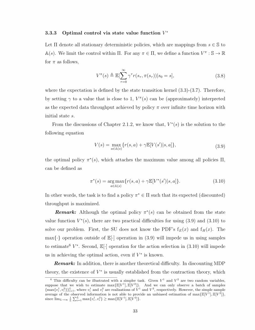
3.3.3 Optimal control via state value function V ∗

Let Π denote all stationary deterministic policies, which are mappings from s ∈ S to

A(s). We limit the control within Π. For any π ∈ Π, we define a function V π : S→ R

for π as follows,

V π(s) , E[∞∑τ=0

γτr(sτ , π(sτ ))|s0 = s], (3.8)

where the expectation is defined by the state transition kernel (3.3)-(3.7). Therefore,

by setting γ to a value that is close to 1, V π(s) can be (approximately) interpreted

as the expected data throughput achieved by policy π over infinite time horizon with

initial state s.

From the discussions of Chapter 2.1.2, we know that, V ∗(s) is the solution to the

following equation

V (s) = maxa∈A(s)

r(s, a) + γE[V (s′)|s, a], (3.9)

the optimal policy π∗(s), which attaches the maximum value among all policies Π,

can be defined as


r(s, a) + γE[V ∗(s′)|s, a]. (3.10)

In other words, the task is to find a policy π∗ ∈ Π such that its expected (discounted)

throughput is maximized.

Remark: Although the optimal policy π∗(s) can be obtained from the state

value function V ∗(s), there are two practical difficulties for using (3.9) and (3.10) to

solve our problem. First, the SU does not know the PDF’s fE(x) and fH(x). The

max· operation outside of E[·] operation in (3.9) will impede us in using samples

to estimate6 V ∗. Second, E[·] operation for the action selection in (3.10) will impede

us in achieving the optimal action, even if V ∗ is known.

Remark: In addition, there is another theoretical difficulty. In discounting MDP

theory, the existence of V ∗ is usually established from the contraction theory, which

6 This difficulty can be illustrated with a simpler task. Given V 1 and V 2 are two random variables,suppose that we wish to estimate maxE[V 1],E[V 2]. And we can only observe a batch of samplesmaxv1

i , v2i Li=1, where v1

i and v2i are realizations of V 1 and V 2, respectively. However, the simple sample

average of the observed information is not able to provide an unbiased estimation of maxE[V 1],E[V 2],since limL→∞

1L

∑Li=1 maxv1

i , v2i ≥ maxE[V 1],E[V 2].

33

requires the reward function r(s, a) to be bounded for all s and all a [49, p. 143].

However, this is not satisfied in our approach, since we allow the channel gain h to

take all positive values, and hence, r is unbounded over the state space. Therefore,

in this case, the existence of V ∗ is not easy to establish.

As we will show in Section 3.4, both the practical and theoretical difficulties can

be solved by transforming the value function into an after-state setting. Moreover,

this transformation reduces space complexity via eliminating the explicit need for

representing EH and H processes.

3.4 After-state Reformulation

Here, we first analyze the structure of the two-stage MDP (Section 3.4.1). Second,

Section 3.4.2 reformulates the optimal control in terms of after-state value function

J∗. Finally, the solution of J∗, and its relationships with the state value function V ∗

are given in Section 3.4.3.

3.4.1 Structure of the MDP

The structural properties of the MDP given in the 4-tuple (S, (A(s))s, f(·|s, a), r(s, a))

are as follows.

1) We divide each state into endogenous and exogenous components. Specifically,

for a sensing-probing state sSP , the endogenous and exogenous components are dSP =

[pSP , bSP ] and xSP = eH, respectively. All possible dSP and xSP are defined as DSP

and XSP , respectively.

Similarly, for a transmitting state sT , the endogenous and exogenous components

are dT = bT and xT = h, respectively. All possible dT and xT are DT and XT ,

respectively.

Finally, let d ∈ D = DSP ∪ DT and x ∈ X = XSP ∪ XT .

2) The number of available actions A(s) at each state s is finite.

3) Checking the state transition kernel (3.3), (3.4), (3.5), (3.6) and (3.7), we can

see that, given state s = [d, x], and action a ∈ A(s), the transition to next state

s′ = [d′, x′] has following properties.

• The stochastic model of d′ is fully known. Specifically, for a given action a

34

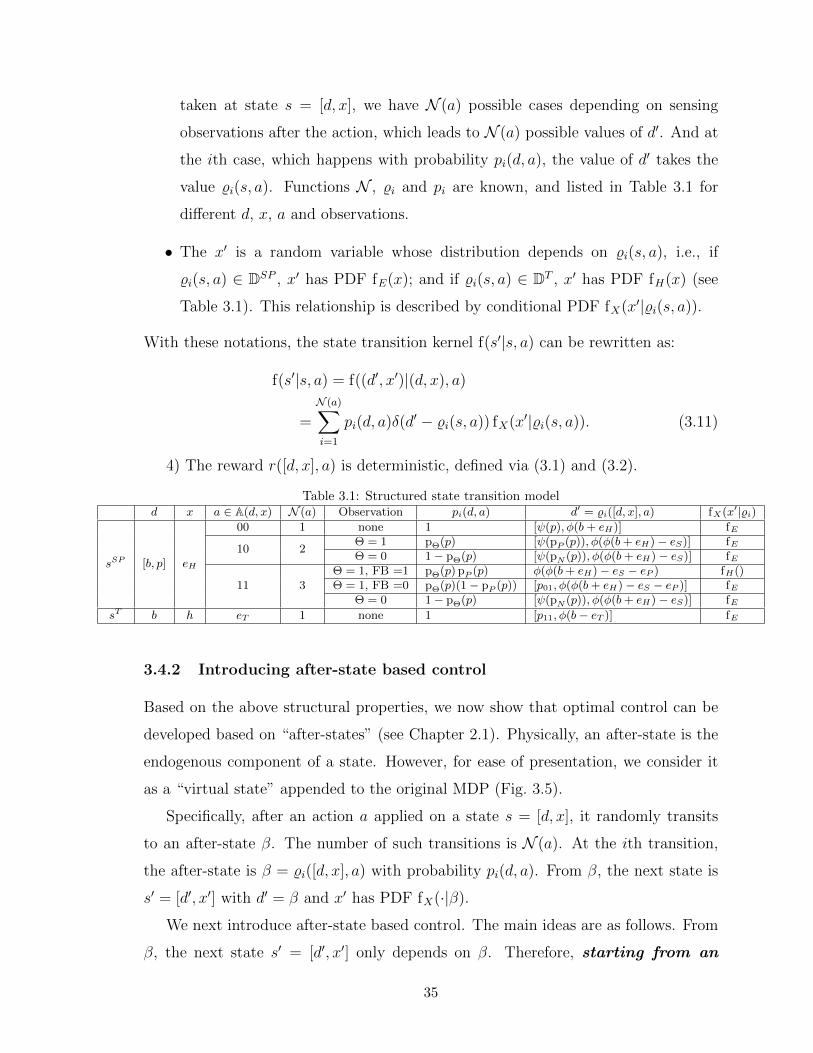
taken at state s = [d, x], we have N (a) possible cases depending on sensing

observations after the action, which leads to N (a) possible values of d′. And at

the ith case, which happens with probability pi(d, a), the value of d′ takes the

value %i(s, a). Functions N , %i and pi are known, and listed in Table 3.1 for

different d, x, a and observations.

• The x′ is a random variable whose distribution depends on %i(s, a), i.e., if

%i(s, a) ∈ DSP , x′ has PDF fE(x); and if %i(s, a) ∈ DT , x′ has PDF fH(x) (see

Table 3.1). This relationship is described by conditional PDF fX(x′|%i(s, a)).

With these notations, the state transition kernel f(s′|s, a) can be rewritten as:

f(s′|s, a) = f((d′, x′)|(d, x), a)

=

N (a)∑i=1

pi(d, a)δ(d′ − %i(s, a)) fX(x′|%i(s, a)). (3.11)

4) The reward r([d, x], a) is deterministic, defined via (3.1) and (3.2).

Table 3.1: Structured state transition modeld x a ∈ A(d, x) N (a) Observation pi(d, a) d′ = %i([d, x], a) fX(x′|%i)

sSP [b, p] eH

00 1 none 1 [ψ(p), φ(b+ eH)] fE

10 2Θ = 1 pΘ(p) [ψ(pP (p)), φ(φ(b+ eH)− eS)] fEΘ = 0 1− pΘ(p) [ψ(pN (p)), φ(φ(b+ eH)− eS)] fE

11 3Θ = 1, FB =1 pΘ(p) pP (p) φ(φ(b+ eH)− eS − eP ) fH()Θ = 1, FB =0 pΘ(p)(1− pP (p)) [p01, φ(φ(b+ eH)− eS − eP )] fE

Θ = 0 1− pΘ(p) [ψ(pN (p)), φ(φ(b+ eH)− eS)] fEsT b h eT 1 none 1 [p11, φ(b− eT )] fE

3.4.2 Introducing after-state based control

Based on the above structural properties, we now show that optimal control can be

developed based on “after-states” (see Chapter 2.1). Physically, an after-state is the

endogenous component of a state. However, for ease of presentation, we consider it

as a “virtual state” appended to the original MDP (Fig. 3.5).

Specifically, after an action a applied on a state s = [d, x], it randomly transits

to an after-state β. The number of such transitions is N (a). At the ith transition,

the after-state is β = %i([d, x], a) with probability pi(d, a). From β, the next state is

s′ = [d′, x′] with d′ = β and x′ has PDF fX(·|β).

We next introduce after-state based control. The main ideas are as follows. From

β, the next state s′ = [d′, x′] only depends on β. Therefore, starting from an

35

Figure 3.5: Augmented MDP model with after-state

after-state β, the maximum expected discounted reward only depends on

β . We denote it by an after-state value function J∗(β). The key is that if J∗(β) is

known for all β, the optimal action at a state s = [d, x] can be determined as

π∗([d, x]) =arg maxa∈A([d,x])

r([d, x], a) +

N (a)∑i=1

pi(d, a)J∗(%i([d, x], a)). (3.12)

The equation (3.12) is intuitive: the optimal action at a state s = [d, x] is the one that

maximizes the sum of the immediate reward r([d, x], a) and the expected maximum

future value∑N (a)

i=1 pi(d, a)J∗(%i([d, x], a)). The solving of J∗ and the formal proof of

(3.12) are provided in Section 3.4.3.

Remark: Unlike (3.10), if J∗ is known, generating actions with (3.12) is easy,

since N (a) and |A(s)| are finite, and pi(d, a) and %i([d, x], a) are known. Furthermore,

the space complexity of J∗ is lower than that of V ∗, since X does not need to be

represented in J∗.

3.4.3 Establishing after-state based control

The development of this subsection is as follows. First, we define a so-called after-

state Bellman equation as

J(β) = γ EX′|β

[max

a′∈A([β,X′])r(β,X ′, a′) +

N (a′)∑i=1

pi(β, a′)J(%i([β,X

′], a′))], (3.13)

where EX′|β

[·] means taking expectation over random variable7 X ′, which has PDF

fX(·|β). Then, Theorem 3.1 shows that (3.13) has a unique solution J∗, and also

provides a value iteration algorithm for solving it. Note that, at this moment, the

7 Given that the after-state of current slot is β, X ′ denotes the random exogenous variable of the nextslot (see Fig. 3.5).

36

meaning of J∗ is unclear. Finally, Theorem 3.2 and Corollary 3.1 show that J∗ is

exactly the after-state value function defined in Section 3.4.2, and the policy defined

with (3.12) is equivalent with (3.10), and therefore, is the optimal policy.

Theorem 3.1. Given Assumption 3.1, there is a unique J∗ that satisfies (3.13).

And J∗ can be calculated via a value iteration algorithm: with J0 being an arbitrary

bounded function, the sequence of functions JlLl=0 defined by the following iteration

equation: for all β ∈ D,

Jl+1(β)← γ EX′|β

[ maxa′∈A([β,X′])

r([β,X ′], a′) +

N (a′)∑i=1

pi(β, a′)Jl(%i([β,X

′], a′))], (3.14)

converges to J∗ when L→∞.

Proof. See Section 3.8.1.

Remark: Unlike the classical Bellman equation (3.9), in the after-state Bellman

equation (3.13), the expectation is outside of the reward function. While this is

unbounded, its expectation is bounded due to Assumption 3.1. Therefore, the solution

to (3.13) can be established by contraction theory.

Remark: Comparing with (3.9), equation (3.13) exchanges the order of (condi-

tional) expectation and maximization operators. And inside the maximization oper-

ator, functions r, N , pi, and %i are known. These are crucial in developing a learning

algorithm that uses samples to estimate the after-state value function J∗.

Theorem 3.2. The existence of a solution V ∗ to (3.9) can be established from J∗.

In addition, their relationships are

V ∗([d, x]) = maxa∈A([d,x])

r([d, x], a) +

N (a)∑i=1

pi(d, a)J∗(%i([d, x], a))

(3.15)

and

J∗(β) = γ EX′|β

[V ∗([β,X ′])] . (3.16)


Corollary 3.1. J∗ is the after-state value function, and the policy defined with (3.12)

is optimal.

37

Proof. From (3.16) and the physical meaning of V ∗ (see (2.4) in Chapter 2.1), J∗(β)

represents the maximum expected discounted sum of reward, starting from after-state

β. Therefore, J∗ is the after-state value function.

The equation (3.12) can be derived from the optimal policy (3.10) as follows: first

decompose the expectation with (3.11), and then plug in (3.16). Therefore, (3.12) is

the optimal policy.

Corollary 3.1 shows that optimal control can be achieved equivalently through

value function J∗. And Theorem 3.1 establishes the existence of J∗ and also pro-

vides a value iteration algorithm for solving J∗. However, there are two difficulties

in obtaining J∗ using the value iteration algorithm. Difficulty 1: the computa-

tion of EX′|β

[·] requires the knowledge of fE and fH , which is unknown in our setting.

Difficulty 2: the after-state space D is continuous, which requires computation of ex-

pectation at infinitely many β. Through reinforcement learning, these two difficulties

will be addressed in Section 3.5.

3.5 Reinforcement Learning Algorithm

In this section, we first address Difficulty 2 via discretizing the after-state space into

finite clusters, which is discussed in Section 3.5.1. In addition, a learning algorithm

is proposed in Section 3.5.2 to address Difficulty 1. Given data samples of wireless

channel and energy-harvesting process, the algorithm learns a (near) optimal policy

via sample averaging, instead of taking expectation. Furthermore, the algorithm’s

convergence guarantee and performance bounds are analyzed in Section 3.5.3. Finally,

the algorithm is modified in Section 3.5.4, for achieving simultaneous data sampling,

learning and control.

3.5.1 After-state space discretization

We will divide the continuous after-state space D into a finite number of portions or

clusters K, which defines a mapping ω : D→ K. In addition, all after-states assigned

into the same cluster are mapped into one representative after-state. Mathematically,

let D(k) , β ∈ D|ω(β) = k denote the set of after-state assigned to cluster k ∈ K.

Thus, q(k) ∈ D(k) represents all after-states of D(k). Finally, we denote KSP as the

38

image of DSP under ω with its elements denoted as kSP . And we denote KT as the

image of DT under ω with its elements denoted as kT .

As an example, in Fig. 3.6, two-dimensional DSP is uniformly discretized into

9 clusters KSP = 1, ..., 9. The one-dimensional subset of after-state space DT is

uniformly discretized into 3 clusters KT = 10, 11, 12. The association from an

after-state β to the cluster k is denoted by k = ω(β). And the after-states assigned

to the same cluster are represented by its central point, q(k).

Figure 3.6: An example of after-state space discretization

3.5.2 Learn optimal policy with data samples

With this discretization, we design a reinforcement learning algorithm that learns

near optimal policy from the samples of EH and H.

The idea is to learn a function g(x) over K to approximate J∗(x) such that g(ω(β))

is close to J∗(β) for all β ∈ D. Then a near-optimal policy can be constructed as

π([d, x]|g) = arg maxa∈A([d,x])

r([d, x], a) +

N (a)∑i=1

pi(d, a)g(ω(%i([d, x], a)). (3.17)

Comparing (3.17) with (3.12), we observe that if g(x) approximates J∗(x) accurately,

π(·|g) is close to π∗.

The function g(x) is learned by iteratively updating with data samples. Each

update uses only one data sample. This facilitates the tailoring of the algorithm for

online applications (Section 3.5.4). Next, we present the algorithm and some intuitive

reasons.

39

3.5.2.1 Algorithm

Initial with arbitrary bounded function g0(x). Calculate gl+1(x) from gl(x) and xl,

the lth data sample. Since xl can be either an energy or fading sample, there are two

cases:

• if xl is a sample of EH , randomly choose N non-repeated clusters from KSP ;

• if xl is a sample of H, randomly choose N non-repeated clusters from KT .

For either case, we denote the set of chosen clusters as Kl. Given xl and Kl, we have

the updating rule as

gl+1(k) =

(1− αl(k)) · gl(k) + αl(k) · δl(k) k ∈ Kl

gl(k) otherwise,(3.18)

where αl(k) ∈ (0, 1) is the step size of cluster k for the lth iteration, and δl(k) is

constructed with xl as

δl(k) , γ maxa∈A([q(k),xl])

r([q(k), xl], a) +

N (a)∑i=1

pi(q(k), a)gl(ω(%i([q(k), xl], a))) (3.19)

(see Section 3.5.2.2 for the interpretation of δl(k)).

Section 3.5.3 will show that if energy and fading can be sampled infinitely often,

the step size αl(k) decays and the sequence of functions gl(x)∞l=1 converges such

that g∞(ω(β)) is close to J∗(β), and the policy π(·|g∞) defined (3.17) is close to π∗.

Algorithm 3.1 Learning of control policy

Require: Data samples xllEnsure: Learned control policy π(·|gL)

Initialize g0(k) = 0, ∀kfor l from 0 to L− 1 do

if xl is a data sample of EH thenChoose N clusters from KSP and get K l

else if xl is a data sample of H thenChoose N clusters from KT and get K l

end ifGenerate gl+1 by executing (3.18) with (xl, K l)

end forWith gL, construct control policy π(·|gL) through (3.17)

The above algorithmic pieces are summarized in Algorithm 3.1. For a sufficiently

large L number of iterations, the learning process can be considered complete. The

40

learned policy π(x|gL) can then be used for sensing, probing and transmission control,

just as in Algorithm 3.2 in Section 3.5.48.

3.5.2.2 Intuitions

Algorithm 1 is a stochastic approximation algorithm [76], which is intuitively gener-

alization of the value iteration algorithm (3.14). Specifically, it is known from (3.14)

that, given the value function Jl(β) of the l-th iteration, a noisy estimation of Jl+1(β)

can be constructed as

maxa′∈A([β,x′])

r([β, x′], a′) +

N (a′)∑i=1

pi(β, a′)Jl(%i([β, x

′], a′)), (3.20)

with x′ sampled from fX(·|β), i.e., x′ is a realization of EH , if β ∈ DSP ; and x′ is a

realization of H, if β ∈ DT .

Therefore, by comparing (3.20) with (3.19), we see δl(k) as an estimate of gl+1(k)

for k ∈ Kl (with ω introduced for discretization, β approximated with q(k), and Jl

replaced with gl). Hence, with δl(k), equation (3.18) updates gl+1 for chosen clusters

within Kl by sample averaging. Note that, theoretically, we can set Kl to KSP or KT

(xl is energy or fading sample), which could accelerate learning speed (Section 3.6.2.2

gives an example). However, large |KSP | or |KT | leads to increased computations.

Hence, instead of updating all clusters of KSP or KT , we randomly update N clusters

within them at each iteration, which controls the computational burden.

3.5.3 Theoretical soundness and performance bounds

In this part, we formally state the convergence requirements and performance guar-

antees for Algorithm 3.1.

First, for ∀ k ∈ K, we define M(k) = l ∈ 0, 1, ..., L− 1|k ∈ K l, which presents

the set of iteration indices where k is chosen during learning. In addition, we define

ξ , maxk supβ∈D(k)

|J∗(β)− J∗(q(k))|, (3.21)

which describes the “error” introduced by the after-state space discretization. Finally,

in order to evaluate the performance of a policy π from after-states’ point of view,

8 Specifically, we can get an adaptive MAC routine with π(·|gL), by removing lines (2), (5-7), (10-16),and (20-22) of the Algorithm 3.2, and replacing π(·|gl) in line (9) and line (25) with π(·|gL).

41

we define

Jπ(β) = γ EX′|β

[V π([β,X ′])] , (3.22)

where V π is defined in (3.8).

Given the definitions of M(k), ξ and Jπ(β), we have following theorem.

Theorem 3.3. Given that Assumption 3.1 is true, and also assuming that, in Algo-

rithm 3.1, as L→∞, ∑l∈M(k)

αl(k) =∞, ∀k (3.23)

∑l∈M(k)

α2l (k) <∞, ∀k (3.24)

then we have:

(i) the sequence of functions glLl=0 generated in (3.18) converge to a function g∞

with probability 1 as L→∞;

(ii) ||J∗ − J∞|| ≤ ξ1−γ , where function

J∞(β) , g∞(ω(β)), (3.25)

and || · || denotes the maximum norm;

(iii) ||J∗ − Jπ∞|| ≤ 2γξ(1−γ)2 , where

π∞ , π(·|g∞). (3.26)


Remark: Assumptions (3.23) and (3.24) actually put constraints on both xlland αl(k):

(a) Energy-harvesting and wireless fading processes need to be sampled infinitely

often in xlL−1l=0 , as L→∞;

(b) for any k, the sequence of step sizes αl(k)l∈M(k) should delay at a proper rate

(neither too fast nor too slow).

42

For Algorithm 3.1 to converge, the constraint (a) is needed to gain sufficient infor-

mation on random processes; the constraint (b) is needed to properly average out

randomness (small enough step sizes) and make sufficient changes to functions gllvia updating (large enough step sizes). The reasoning from assumptions (3.23) and

(3.24) applying to these two constraints is as follows.

First,∑

l∈M(k) αl(k) = ∞ requires |M(k)| = ∞, where |M(k)| denotes the size

of M(k). Because, otherwise, we have∑

l∈M(k) αl(k) ≤ |M(k)| (as αl(k) is upper

bounded by 1). This further implies the constraint (a), due to the definition of M(k)

and the way that Algorithm 3.1 constructs Kl.

Second, in order to satisfy∑

l∈M(k) α2l (k) <∞, the sequence of step size αl(k)l∈M(k)

should start to delay after certain l with sufficient delay rate. However, the delay rate

should not too large, in order to satisfy∑

l∈M(k) αl(k) = ∞. In summary, we have

the constraint (b) for step size sequences. There are various step size rules that sat-

isfy this constraint [77, Chapter 11]. For example, we can set αl(k) = 1|M(k,l)| , where

M(k, l) is the set of slots that cluster k is chosen before the lth iteration.

Remark: The statement (i) of Theorem 3.3 demonstrates the convergence guar-

antee of Algorithm 1. The statement (ii) shows that the learned function g∞ is close

to the J∗, and their difference is controlled by the error ξ caused by after-state space

discretization. The statement (iii) claims that asymptomatically, the performance of

policies π(·|gl)l approaches that of the optimal policy π∗, and that the performance

gap is proportional to the error ξ.

3.5.4 Simultaneous sampling, learning and control

Algorithm 3.1 operates offline — batch learning which generates the best predictor

by learning on the entire training data set of energy-harvesting and channel fading

data at once. Thus, the optimal policy cannot be used until learning is complete.

However, for some applications, an online learning scheme may be more desirable.

In online machine learning, sequential data is used to update the best predictor for

future data at each step. It is also used in situations where it is necessary for the

algorithm to dynamically adapt to new patterns in the data.

One intuitive idea to tailor Algorithm 3.1 for online learning is as follows. Sup-

posing that current learned function is gl, we can use π(·|gl) to generate actions and

43

interact with the environment in real-time. Thus, we can collect a data sample from

energy-harvesting or channel fading process, which can be further used to generate

gl+1. As the loop continues, gl approaches g∞, and the policy π(·|gl) approaches

π∞, which implies that generated actions during the process will be more and more

likely to be optimal. In this way, simultaneous sampling, learning and control can be

achieved.

However, the problem is that the above method cannot guarantee to sample the

wireless fading process infinitely-often (i.e., cannot satisfy assumptions (3.23) and

(3.24) of Theorem 3.3). Note that the wireless fading process can be sampled only

if π(·|gl) chooses aSP = 11. But, the above method may enter a deadlock such that

aSP = 11 will never be chosen. The deadlock can be caused by: (1) insufficient

battery energy that results from the learned policy’s consistent aggressive use of

energy; and/or (2) persistently locking in aSP = 00 or aSP = 10. In order to break

this possible deadlock during the learning process, with some small probability ε

(named as the exploration rate), we force the algorithm to deviate from π(·|gl) to

either accumulate energy (aSP = 00) or to probe channel gain information (aSP = 11)

(e.g., exploration).

Based on the above points, Algorithm 3.2 is provided for always-on sampling,

learning and control. Here, we argue that gl generated by Algorithm 3.2 converges

to g∞ when t → ∞. First, at each time slot, there is probability ε/2 that the

algorithm will choose aSP = 00 to accumulate energy. Therefore, given the battery

level bSPt of slot t, we can9 find a finite T such that probbSPt+T ≥ eS + eP > 0. In

other words, at any slot t ≥ T , we have probbSPt ≥ eS + eP > 0. Thus, having

sufficient energy for sensing and probing, the algorithm will choose aSP = 11 with

probability ε/2. In addition, at any time slot, the channel will be free with a non-zero

probability. Therefore, there is a non-zero probability that the algorithm can reach

the transmitting stage. Thus, the wireless fading process can be sampled infinitely

often for t→∞. In summary, the assumptions (3.23) and (3.24) of Theorem 3.3 are

satisfied (under properly delayed step size), and gll converges to g∞ asymptotically.

9 If this condition cannot be satisfied, the underlying energy harvest process is not sufficient to powersecondary nodes.

44

Algorithm 3.2 Simultaneous sampling, learning and control

Note: βSPt ∈ DSP presents an after-state in slot t. βTt is defined similarly.1: Initialize: battery b0, channel belief p0, and after-state βSP0 = [b0, p0]2: Initialize: g0(k) = 0, ∀k, and set l = 03: for t from 1 to ∞ do4: Observe arriving harvested energy amount eHt5: Set xl = eHt and choose K l with N clusters from KSP

6: Generate gl+1 by executing (3.18) with (xl, K l)7: l← l + 18: Construct state sSPt = [βSPt−1, eHt]9: Generate sensing-probing decision aSPt = π(sSPt |gl) via (3.17)

10: if random() ≤ ε then . Exploration11: if random() ≤ 1/2 then12: aSPt = 0013: else if 11 ∈ A(sSPt ) then . Energy sufficiency14: aSPt = 1115: end if16: end if17: Apply sensing and probing actions based on aSPt18: if aSPt = 11 & Θ = 1 & FB = 1 then19: Observe the channel gain ht from FB20: Set xl = ht, and construct K l by choosing N clusters from KT

21: Generate gl+1 by executing (3.18) with (xl, K l)22: l← l + 123: Derive after-state βTt with sSPt via Table 3.124: Construct state sTt = [βTt , ht]25: Generate transmit decision aTt = π(sTt |gl) via (3.17)26: Set transmission power based on aTt , and transmit data27: Derive after-state βSPt from (sTt , a

Tt ) via Table 3.1

28: else29: Derive after-state βSPt with sSPt and aSPt , Θ and FB via Table 3.130: end if31: end for

45

3.5.4.1 Choices of exploration rate

Although the convergence is guaranteed for any ε ∈ (0, 1), the choice of ε affects

the performance of the algorithm. Large ε helps channel acquisition, which may in

turn accelerate the learning process. But too large ε will make the algorithm act too

randomly, and cause significant loss to the achievable performance. Section 3.6.2.1

discusses the choice of ε in detail.

3.5.4.2 Complexity analysis of Algorithm 3.2

For each t, major computations are the two embedded function updates for gl (line 6

and line 21). Each update needs to compute (3.19) N times. And each computation

requires |N (a)| multiplications, |N (a)| summations and one maximization over a set

with size |A(a)|.

3.5.4.3 Energy burden for running Algorithm 3.2

In this part, we consider the energy burden for executing Algorithm 3.2 within each

time slot, since it is running on an energy limited node. The exact amount of energy

consumption is difficult to compute, since it depends on hardware platforms and

algorithm implementation details. Hence, we roughly estimate the order of energy

consumption (rather than its exact value).

Reference [78] shows that the energy consumption for executing of an algorithm

is determined as

Engyalg = Ppro · Talg,

where Ppro is the operating power of the processor (where the algorithm is executed)

and Talg is the time needed for executing the algorithm. In addition, Talg can be

modeled as

Talg = Calg ·1

fpro

,

where fpro is the clock frequency of the processor, and Calg denotes the number of

clocks that the processor needs to execute to the algorithm within each time slot.

Assuming that |ET| = 6 and N = 1, from Section 3.5.4.2 and Table 3.1, we know

that, in worst case, executing Algorithm 3.2 requires 4 multiplications, 4 summations,

46

one maximization over a set with size 3 and one maximization over a set with size 6.

It is sensible to assume that Calg is with order 102. Furthermore, reference [79] shows

that, for modern processors, Ppro

fprois with order 10−9 Joule. In summary, the order of

Engyalg should be around 10−7 Joule.

Therefore, within each time slot, energy consumption for executing learning algo-

rithm is negligible compared with that for sensing, probing and transmitting. For ex-

ample, a typical transmission power is around 10 mW, and packet duration is around

10 ms, which means that the typical transmission energy is around 10−4 Joule.

3.6 Simulation Results

3.6.1 Simulation setup

The secondary signal power attenuation h consists of path loss hs and channel fading

hf . We assume a Rayleigh fading model. Thus, hf has PDF f(x) = e−x, x ≥ 0.

The path loss hs is distance-dependent and is assumed to be fixed.

Then, with above channel model, the amount of transmitted data can be rewritten

as

τTW log2(1 +eThshfτTN0W

) = τTW log2(1 +eThfη

)

where η , τTN0W/hs. We assume that W = 1 MHz, τT = 10 ms, and η = 1

(for energy normalization). Normalizing with respect to η, we set battery capacity

Bmax = 10, sensing energy eS = 1, probing energy eP = 1, and the set of transiting

energy levels ET = 0, 1, 2, 3, 4, 5.

In addition, we assume that energy is harvested from wind power. Thus, EH is

well characterized by the Weibull distribution [80], with shape and mean parameters

kE and µE. Throughout the simulation, we set kE = 1.2, and change µE to model

different harvested energy supply rates.

Furthermore, the channel occupancy Markov model is described by p00 = 0.8 and

p11 = 0.9 and spectrum sensing are set as: pFA = 0.1 and pM = 0.01.

Finally, simple uniform grid is used for discretization with 10 levels each for both

belief and battery dimensions. Thus, |KSP | = 100 and |KT | = 10.

47

3.6.2 Characteristics of online learning algorithm

3.6.2.1 Learning under various exploration rate ε

With µE = 1 and the update size N = 1, we investigate Algorithm 3.2 for ε ∈

10−5, 10−4, 10−3, 10−2, 10−1 and for ε adapting with√

1/t.

100

101

102

103

104

105

106

107

0

0.02

0.04

0.06

0.08

0.1

0.12

0.14

Av

erag

e D

ata

Rat

e (M

bp

s)

Figure 3.7: Learning curves under various exploration rates

Fig. 3.7 shows the learning curves with logarithmic time index. Note that smaller

ε takes longer time to initiate the learning process. In addition, some learning curves

(with ε equal to 10−1, 10−2, 10−3 and√

1/t) consist of an initial phase (from 0 to

around 105 steps) and a final phase, which begins (at around the 105-th step) with a

steep performance increase. These phenomena are explained as follows.

First, note that ε determines the frequency of sampling of the wireless fading

process, which further determines the updating rate of gl(x) over KT . In addition,

the learning complexity for transmitting policies is much lower than that for sensing-

probing policies, since the size of KT (e.g., 10) is much smaller than that of KSP

(e.g., 100). Therefore, with large enough ε (equal to 10−1, 10−2, 10−3 and√

1/t), the

transmitting policy learns significantly faster than the sensing-probing policy. Hence,

the learning curve manifests a two-phase process. And since larger ε implies obtaining

CSI more often, an algorithm with larger ε initiates faster.

48

However, having too large a value for ε can cause performance loss due to too

aggressive exploration. For example, for ε = 10−1, the system achieves 10% less

throughput than in other cases. As well, ε =√

1/t, which starts with large value

and decreases over time, provides fast start-up and also almost-lossless asymptotic

performance.

3.6.2.2 Learning with update size N

With µE = 1 and ε =√

1/t, we investigate Algorithm 3.2 for N ∈ 1, 2, 5, 10.

We observe that all algorithms converge to the same limit (Fig. 3.8), but larger N

requires fewer learning steps. This suggests a trade-off between computational load

and learning speed.

103

104

105

106

107

0.09

0.1

0.11

0.12

0.13

0.14

Figure 3.8: Learning curves under various update sizes

3.6.3 Myopic versus holistic

We next compare Near Opt (the policy learned by Algorithm 3.2), Greedy-Sensing-

Probing (GSP), Greedy-Transmitting (GT), and Greedy-Sensing-Probing-Transmitting

(GSPT). GSP always senses and probes the channel, but adapts the transmit power,

which is learned by constraining the action space A(s) in (3.19) and (3.17) to have

only the greedy action at sensing-probing states. In GT, which is learned similarly,

the node transmits at maximum power level whenever the energy is sufficient, but

carefully chooses the sensing and probing action. GSPT is a pure greedy policy with

49

myopic actions at both stages. We compare how these policies perform with different

rates of energy harvests (vs. mean harvested energy µE).

1 2 3 4 5 6 7 8 9 10

Mean of Harvested Energy

0

0.1

0.2

0.3

0.4

0.5

0.6

0.7

CH

. A

cces

s P

rob

.

Near Opt

GSP

GT

GSPT

CH. Idle Prob. 10 20 40 60 80 1000.5

0.55

0.6

0.65

0.7

Figure 3.9: Channel access probability under different µE

First, we consider the ability of a policy to exploit channel access opportunities.

This is measured by channel access probability, which is the probability that the

channel is free while a sensing action is chosen. As a benchmark, this probability

is upper bounded by the channel’s idle probability p01/(p01 + p10) = 0.2/0.3 ≈ 0.67.

Fig. 3.9 shows the measured channel access probabilities of different policies. In

addition, the data rate is measured and presented in Fig. 3.10, which is upper-bounded

by p01/(p01 +p10) ·pO ·E[W log2(1+eMT hf )] ≈ 1.285 Mbps, where eMT = maxET = 5.

Overall, all the policies exploit the increasing harvested energy for more channel

access opportunities and higher data rates. And with a high enough energy supply,

all the policies achieve the upper bounds.

Note that GSPT is most efficient at exploiting channel access opportunities be-

cause it is aggressive in sensing and probing. However, the drawback is that these

actions are energy intensive, resulting in a lack of energy for data transmission. Thus,

GSPT has the worst performance in terms of data rate.

Compared with GSPT, GSP has lower channel access probability but achieves

a higher data rate. The main reason is that GSP adapts transmit power based on

channel fading status and the greedy sensing-probing strategy. Therefore, GSP uses

50

1 2 3 4 5 6 7 8 9 10

Mean of Harvested Energy

0

0.2

0.4

0.6

0.8

1

1.15

Aver

age

Dat

a R

ate

(Mbps)

Near Opt

GSP

GT

GSPT

Max Rate

10 20 40 60 80 1000.95

1

1.1

1.2

1.3

Figure 3.10: Data rates for different µE

energy more efficiently for data transmitting rather than simply sensing and probing.

In contrast, GT always uses the highest transmit power without considering the

channel status. And this policy strives to make intelligent sensing and probing de-

cisions based on battery energy level, channel belief and the aggressive transmission

strategy. When the harvested energy is low, GT outperforms GSP in terms of data

rate. That is because making proper sensing and probing decision to save energy

for transmission is far more important. However, when the harvested energy supply

increases, GSP outperforms GT. The reason is that energy expenses due to greedy

sensing and probing action are marginal relative to the available energy.

With full adaptation, Near Opt achieves favorable energy trade-offs between sensing-

probing and transmission stages. Therefore, Near Opt achieves the best data rate.

3.7 Summary

In this chapter, with goal of maximizing data throughput, we studied the optimal

design of spectrum sensing, channel probing and transmitting for energy-harvesting

cognitive nodes. The optimal control problem was formulated with a two-stage MDP

model, and further simplified via after-state technique. For addressing the difficulty

of lacking distribution information, we proposed to use reinforcement learning to solve

51

the optimal policy, whose theoretical basis and performance bounds were analyzed.

3.8 Appendix

3.8.1 Proof of Theorem 3.1

Theorem 3.1 is proved with the use of contraction theory. Specifically, we show the

solution to (3.13) uniquely exists, and it is the fixed point of a contraction mapping.

Furthermore, the value iteration algorithm (3.14) converges to the fixed point.

First, define the set of bounded functions J : D → R as F. Then, let T ∗ be an

operator on F, and for any J ∈ F, T ∗J is another function with domain D, whose

value at β is defined as

(T ∗J)(β) = γ EX′|β

[ maxa′∈A([β,X′])

r([β,X ′], a′) +

N (a′)∑i=1

pi(β, a′)J (%i([β,X

′], a′))].

By Assumption 3.1, it is easy to check that, given J is bounded, T ∗J is bounded (i.e.,

T ∗J ∈ F). Therefore, T ∗ is a mapping from F to F. It is shown in [81, p. 211] that F

is complete under the maximum norm. Furthermore, as shown in the following, T ∗

is a contraction mapping under the maximum norm with modulus γ. Therefore, the

contraction theory applies to T ∗.

Due to the contraction theory [81, p. 209], there exists a unique fixed point for T ∗,

denoted as J∗, such that T ∗J∗ = J∗, i.e., function J∗ does not change under operator

T ∗. Note that equation T ∗J∗ = J∗ is exactly the after-state Bellman equation (3.13).

Therefore, we have shown that there is a unique solution to (3.13).

In addition, the contraction theory [81, p. 209] states that, for arbitrary function

J0 ∈ F, liml→∞

T ∗lJ0 = J∗. Note that T ∗lJ0 means the function that is generated by,

starting from J0, iteratively applying operator T ∗ on previously generated function

for l times, which exactly describes the value iteration algorithm (3.14). This has

proved the value iteration algorithm (3.14) converges to J∗.

Hence, there only remains to show that T ∗ is a contraction mapping. Given any

two functions J1, J2 ∈ F, for β that satisfies (T ∗J1)(β) ≥ (T ∗J2)(β), we have

0 ≤ (T ∗J1)(β)− (T ∗J2)(β)

= γ EX′|β

[max

a1∈A([β,X′])

r([β,X ′], a1) +

N (a1)∑i=1

pi(β, a1)J1(ρi([β,X′], a1))

52

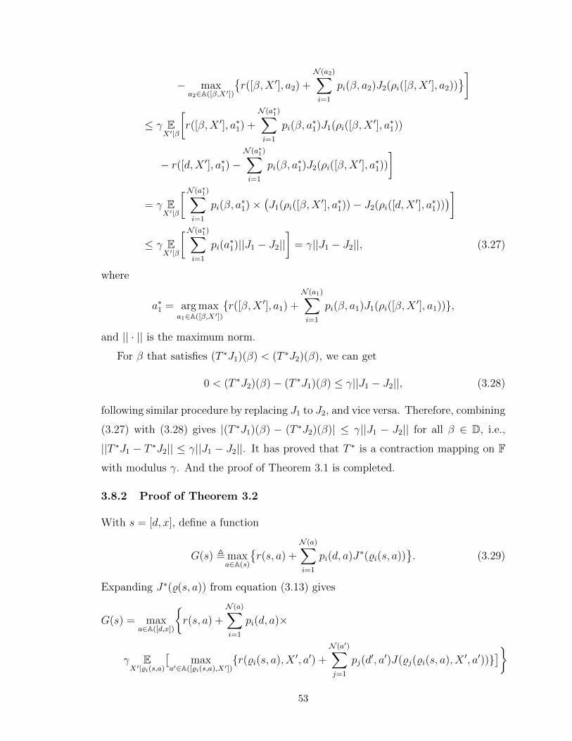
− maxa2∈A([β,X′])

r([β,X ′], a2) +

N (a2)∑i=1

pi(β, a2)J2(ρi([β,X′], a2))

]

≤ γ EX′|β

[r([β,X ′], a∗1) +

N (a∗1)∑i=1

pi(β, a∗1)J1(ρi([β,X

′], a∗1))

− r([d,X ′], a∗1)−N (a∗1)∑i=1

pi(β, a∗1)J2(ρi([β,X

′], a∗1))

]

= γ EX′|β

[N (a∗1)∑i=1

pi(β, a∗1)×

(J1(ρi([β,X

′], a∗1))− J2(ρi([d,X′], a∗1))

)]

≤ γ EX′|β

[N (a∗1)∑i=1

pi(a∗1)||J1 − J2||

]= γ||J1 − J2||, (3.27)

where

a∗1 = arg maxa1∈A([β,X′])

r([β,X ′], a1) +

N (a1)∑i=1

pi(β, a1)J1(ρi([β,X′], a1)),

and || · || is the maximum norm.

For β that satisfies (T ∗J1)(β) < (T ∗J2)(β), we can get

0 < (T ∗J2)(β)− (T ∗J1)(β) ≤ γ||J1 − J2||, (3.28)

following similar procedure by replacing J1 to J2, and vice versa. Therefore, combining

(3.27) with (3.28) gives |(T ∗J1)(β) − (T ∗J2)(β)| ≤ γ||J1 − J2|| for all β ∈ D, i.e.,

||T ∗J1 − T ∗J2|| ≤ γ||J1 − J2||. It has proved that T ∗ is a contraction mapping on F

with modulus γ. And the proof of Theorem 3.1 is completed.


With s = [d, x], define a function

G(s) , maxa∈A(s)

r(s, a) +

N (a)∑i=1

pi(d, a)J∗(%i(s, a)). (3.29)

Expanding J∗(%(s, a)) from equation (3.13) gives

G(s) = maxa∈A([d,x])

r(s, a) +

N (a)∑i=1

pi(d, a)×

γ EX′|%i(s,a)

[max

a′∈A([%i(s,a),X′])r(%i(s, a), X ′, a′) +

N (a′)∑j=1

pj(d′, a′)J(%j(%i(s, a), X ′, a′))

]

53

= maxa∈A([d,x])

r(s, a) + γ

N (a)∑i=1

pi(d, a) EX′|%i(s,a)

[G(%i(s, a), X ′)]

= maxa∈A([d,x])

r(s, a) + γE [G(S ′)|s, a]

, (3.30)

where the definition of G implies the second equality, and (3.11) implies the last

equality. Note that (3.30) is exactly the state Bellman equation (3.9). Therefore,

function G = V ∗ solves (3.9), and the relationship (3.15) is established. Finally, with

(3.29) and the definition of the after-state Bellman equation (3.13), the relationship

(3.16) is established, which completes the proof.


For Algorithm 3.1, we define two operators H and H. Let H be an operator on

functions K 7→ R. Applying H on a function g, i.e., Hg, gives another function with

domain K, and its value at k is defined as

(Hg)(k) = γ EX′|q(k)

[ maxa′∈A([q(k),X′])

r([q(k), X ′], a′) +

N (a′)∑i=1

pi(q(k), a′)g(ω(%i([q(k), X ′], a′)))].

Similarly, define another operator on functions K 7→ R as

(Hg)(k) = γ maxa′∈A([q(k),X′])

r([q(k), X ′], a′) +

N (a′)∑i=1

pi(q(k), a′)g(ω(%i([q(k), X ′], a′))),

where X ′ is a random variable with PDF fX(·|q(k)). Note that the outcome of Hg is

random, and depends on the realization of X ′.

Note that, in Algorithm 3.1, at any iteration l, gl(k) does not change for k /∈ Kl.

Therefore, the step size value αl(k), ∀k /∈ Kl, does not affect the algorithm. By

defining αl(k) = 0, ∀k /∈ Kl, and with the operators H and H, the updating (3.18)

can rewritten as, ∀k ∈ K:

gl+1(k) = (1− αl(k))gl(k) + αl(k)((Hgl)(k) + wl(k)) (3.31)

where wl(k) = (Hgl)(k)− (Hgl)(k).

3.8.3.1 Proof of statement (i):

Due to the proposition 4.4 of [82, p. 156], we have following lemma.

54

Lemma 3.1. Given following conditions,

(a) H is a contraction mapping under maximum norm;

(b) for all k,∑∞

l=0 αl(k) =∞, and∑∞

l=0 α2l (k) <∞;

(c) for all k and l, E[wl(k)|gl] = 0;

(d) there exist constant C1 and C2 such that E[w2l (k)|gl] ≤ C1 + C2||gl||2;

the sequence of functions gll generated from iteration (3.31) converges to a func-

tion g∞ with probability 1, and the limiting function g∞ satisfying Hg∞ = g∞.

We prove the statement (i) of Theorem 3.3 by checking the four conditions of

Lemma 3.1 as follows. First, the contraction mapping condition (a) of H can be

established in a similar procedure as the proof of Theorem 3.1, and is omitted here.

Then, due to assumptions (3.23) and (3.24) of Theorem 3.3, the condition (b) about

αl is satisfied. In addition, we have E[wl(k)|gl] = 0 via the definition of H and H.

Therefore, the condition (c) is satisfied. Finally, we have to show the condition (d):

the bounded variance property of wl. For given k and l, we define a function as

I(x) =γ maxa′∈A([q(k),x])

r([q(k), x], a′) +

N (a′)∑i=1

pi(q(k), a′)gl(ω(%i([q(k), x], a′))).

With the notation I(x), we have

E[w2l (k)|gl] = E

X′|q(k)

[(I(X ′)− E

Y ′|q(k)[I(Y ′)]

)2∣∣∣∣gl] = EX′|q(k)

[(E

Y ′|q(k)[I(X ′)− I(Y ′)]

)2∣∣∣∣gl]≤ E

X′|q(k)

[(E

Y ′|q(k)[2 max

∣∣I(X ′)∣∣, ∣∣I(Y ′)

∣∣])2∣∣∣∣gl]≤ E

X′|q(k)

[(E

Y ′|q(k)[2|I(X ′)

∣∣])2∣∣∣∣gl]+ EX′|q(k)

[(E

Y ′|q(k)[2∣∣I(Y ′)

∣∣])2∣∣∣∣gl]a©≤ E

X′|q(k)

[(2∣∣I(X ′)

∣∣)2∣∣gl]+ EX′|q(k)

[(2L1 + 2||gl||

)2∣∣gl]b©≤ 8L2 + 8||gl||2 + 8L2

1 + 8||gl||2 = 8(L2 + L21) + 16||gl||2,

where the inequalities a© and b© holds from the Assumption 3.1 and the fact that

(x+y)2 ≤ 2x2 +2y2 for any real value x and y. Therefore, it is proven that E[w2l (k)|gl]

is bounded by 8(L2 + L21) + 16||gl||2, which completes the proof of the statement (i)

of Theorem 3.3.

55

3.8.3.2 Proof of statement (ii):

First, define an partial order for functions K 7→ R as follows. If g1(k) ≤ g2(k), ∀k,

we say g1 ≤ g2. It is easy to check that, given any two functions g1 and g2 satisfying

g1 ≤ g2, we have Hg1 ≤ Hg2.

Then, define a function g(k) , infβ∈D(k)

J∗(β) + ξ1−γ . Applying H on g gives

(Hg)(k) = γ EX′|q(k)

[max

a′∈A([q(k),X′])

r([q(k), X ′], a′) +

N (a′)∑i=1

pi(q(k), a′)g(ω(%i([q(k), X ′], a′))]

a©≤ γ E

X′|q(k)

[max

a′∈A([q(k),X′])

r([q(k), X ′], a′) +

N (a′)∑i=1

pi(q(k), a′)(J∗(%i([q(k), X ′], a′)) +

ξ

1− γ)]

b©= J∗(q(k)) +

γξ

1− γc©≤ inf

β∈D(k)J∗(β) + ξ +

γξ

1− γ= g(k),

where equality a© is due to the definition of g(k), equality b© comes from the after-

state Bellman equation (3.13), and inequality c© is due to the definition of ξ in (3.21).

Therefore, we have (Hg)(k) ≤ g(k) for all k, i.e., Hg ≤ g.

Combining the fact that Hg1 ≤ Hg2, if g1 ≤ g2, with the fact that Hg ≤ g,

we have Hkg ≤ g, where Hk means applying H operator k times. Then, due to

Lemma 3.1 in the proof of statement (i), we have limk→∞

Hkg = g∞ ≤ g, which means

g∞(k) ≤ infβ∈D(k)

J∗(β)+ ξ1−γ , ∀ k. Therefore, we get J∗(β) ≥ g∞(ω(β))− ξ

1−γ , ∀ β. From

the definition of J∞ in (3.25), J∗(β)− J∞(β) ≥ − ξ1−γ , ∀ β, follows.

On the other hand, defining g(k) = supβ∈D(k)

J∗(β) − ξ1−γ and following the similar

procedure, we can prove Hg ≥ g, and therefore, get J∗(β) ≤ g∞(ω(β)) + ξ1−γ . In

turn, it implies J∗(β) − J∞(β) ≤ + ξ1−γ , which completes the proof of statement (ii)

in Theorem 3.3.

3.8.3.3 Proof of statement (iii):

For any policy π, define an operator T π on F as10

(T πJ)(β) =γ EX′|β

[r([β,X ′], π) +

N (π)∑i=1

pi(β, π)J (%i([β,X′], π))], (3.32)

10F is defined in Section 3.8.1.

56

where π inside r, N , pi and %i denoting π([β,X ′]). And from the state transition

kernel (3.11), Jπ∞ as defined by (3.22) can be recursively rewritten as

Jπ∞(β) =γ EX′|β

[r([β,X ′], π∞) +

N (π∞)∑i=1

pi(β, π∞)Jπ∞(%i([β,X′], π∞))].

By comparing with T π in (3.32), we have

T π∞Jπ∞ = Jπ∞ . (3.33)

In addition, similar to the proof of Theorem 3.1, T π can be shown to be a contraction

mapping with modulus γ, which means

||T π∞J1 − T π∞J2|| ≤ γ||J1 − J2|| (3.34)

for any J1 and J2. Besides, from the definitions of π(·|g∞) (i.e., π∞) in (3.17) and J∞

in (3.25), we have (T ∗ defined in Section 3.8.1)

T π∞J∞ = T ∗J∞. (3.35)

Furthermore, from statement (ii) of Theorem 3.3, we have

||J∗ − J∞|| ≤ξ

1− γ. (3.36)

Finally, it is shown in the proof of Theorem 3.1 that

T ∗J∗ = J∗, (3.37)

and

||T ∗J1 − T ∗J2|| ≤ γ||J1 − J2|| (3.38)

for any J1 and J2.

By combining the above results, we have

||Jπ∞ − J∗||a©= ||T π∞Jπ∞ − J∗||b©≤ ||T π∞Jπ∞ − T π∞J∞||+ ||T π∞J∞ − J∗||c©≤ γ||Jπ∞ − J∞||+ ||T ∗J∞ − T ∗J∗||d©≤ γ||Jπ∞ − J∗||+ γ||J∗ − J∞||+ γ||J∞ − J∗||e©≤ γ||Jπ∞ − J∗||+ 2γξ

1− γ, (3.39)

57

where a© is due to (3.33); b© is the triangle inequality; c© comes from (3.34), (3.35)

and (3.37); d© is due to the triangle inequality and (3.38), and e© is due to (3.36).

Finally, from (3.39), we have ||Jπ∞ − J∗|| ≤ 2γξ(1−γ)2 , which proves the statement (iii)

of Theorem 3.3.

58

Chapter 4

Optimal Selective Transmission forEnergy-Harvesting WirelessSensors

4.1 Introduction

Wireless sensor networks, consisting of spatially-dispersed autonomous sensors, can

monitor physical or environmental conditions [38, 39]. Important applications in-

clude environmental monitoring, industrial process monitoring and control, machine

learning, data gathering and many more. Ubiquitous deployment of wireless sensor

networks is thus a key enabler of the Internet of Things [83], where the sensors must

be autonomous with limited energy and computational resources. To aid this goal, the

sensor nodes may be powered by harvested energy [84] from ambient sources (solar,

wind and others [74]). This enhances the energy self-sustainability of the nodes and

consequently, the life time of the network is constrained by hardware limits, not by

battery capacity [14]. Hence, energy-harvesting promises enhanced network lifetime,

as well as a more sustainable evolution of wireless sensor networks.

However, due to finite battery capacity and the randomness of harvested energy,

energy depletion can still occur when a sensor node attempts to transmit packets. To

avoid this, a sensor node can evaluate/quantify the priority of data packets and then

decide whether to send or not. For example, data packets containing information of

enemy attacks [40] or fire alarms [41] may have higher priority. So low-priority packets

may be dropped when available energy is limited, which will allow the sensor to

transmit more important packets in a long term. Such selective transmission strategies

59

were studied by [85, 86] in conventional wireless sensor networks and extended to

energy-harvesting settings in [87–90].

In [85], a sensor node considers its available energy and the priority of a packet to

decide whether the packet should be transmitted or not. This policy maximizes the

expected total priority of transmitted packets by the sensor. To enhance this process,

work [86] adds a success index, a measure of the likelihood that a transmitted packet

reaches its destination, e.g., a sink node. Therefore, when making its transmission

decision, each sensor takes decisions of other sensors into consideration through the

use of the success indices, which may improve overall performance. Nevertheless, the

use of success indices introduces communication overhead, as the success index for

each packet has to be passed from the sink node to all sensors along the packet’s

routing path.

Works [87–90] studied selective transmission in energy-harvesting wireless sensor

networks. In [87], the harvested energy of a sensor is modeled as a random variable

that takes value of 0 or 1, and the energy expense for each packet transmission

is always defined as one. Given these assumptions, the sensor’s battery dynamic

can be analyzed by the Markov chain theory, which is then used to develop the

transmission policy. Using the same assumptions on energy-harvesting and energy

expense, work [88] derived the optimal transmission policy. In addition, work [88]

proposed a low-complexity balanced policy: if the priority of a packet exceeds a pre-

defined threshold, it is transmitted. Balanced policy is designed to ensure that the

expected energy consumption equals the expected energy-harvesting gain, leading to

energy neutrality. This ensures energy use efficiency while reducing energy outage

risks. Work [89] extended the result of [88] to the case where there exists temporal

correlation in the energy-harvesting process.

However, in order to find optimal and/or heuristic policies, the statistical distri-

butions of data priority and/or energy-harvesting process are needed in [85–89]. In

addition, works [87–89] assumed one unit of energy for both energy replenishment

and energy consumption, which may not be practical. These two limitations are re-

solved in [90]. Specifically, this work models harvested energy and wireless fading as

general random variables. In addition, based on the Robbins-Monro algorithms [76],

work [15] learns the optimal transmission policy from the observed data, without their

60

statistical distributions.

4.1.1 Motivation, problem statement and contributions

In existing works [85–90], the selective transmission control is made based on energy

status and packet priority, whereas the effect of fading on optimal decision making

has not been considered. Thus, when it is decided to transmit, the transmission may

fail due to wireless fading.

On the other hand, it can be beneficial via incorporating channel status into

decision making. Specifically, based on channel state information (CSI), a node can

estimate the necessary transmission power for achieving reliable communication. The

node may choose not to transmit for energy saving, if CSI indicates the occurrence

of deep fading. The node may also take the advantage of good channel status by

transmitting with lower power. Therefore, selective transmission with CSI exploited

may have more efficient use of energy, compared with those policies in [85–90].

Note that, for obtaining CSI, the node must estimate the wireless channel and

thus sends pilot signals to the receiver side and receives feedback from it. Considering

that the length of the pilot signals is much shorter than that of the data packets [91],

the energy required for channel estimation is small compared to that required for

data transmission. Moreover, for slowly-fading quasi-static channels, which are quite

typical in wireless sensor networks, the channel estimation can be done less frequently.

With aforementioned motivations, we consider selective transmissions of a wireless

sensor node, to optimize its energy usage and to exploit CSI. The node decides to send

or not to send by considering battery status, data priority and fading status, whereas

only the first two factors are considered in [85–90]. In addition, we assume that the

node does not know the statistical distribution of the battery status, data priority, or

fading status. This lack of distributional knowledge must therefore be reflected in the

solving of optimal transmission policy. Considering all the aforementioned challenges,

we make the following contributions.

a) We model the selective transmission problem as a continuous-state MDP [49] (also

see Chapter 2.1). The optimal policy is derived from an after-state value function.

This approach transforms the three-dimensional control problem (i.e., on battery

61

status, priority, and fading status) to a one-dimensional after-state function prob-

lem (i.e., on the “after-state” battery status). As a result, control of transmission

is greatly simplified.

b) The structural properties of the after-state value function and the optimal policy

are analyzed. We prove that the after-state value function is differentiable and

non-decreasing, and that the optimal policy is threshold-based with respect to

data priority and channel status.

c) To address the difficulty of representing the continuous after-state value function,

we find a representational approximation. For preserving the discovered structural

properties, we propose to use a monotone neural network (MNN) [92], and prove

that it is a well-designed approximation for the after-state value function, which

is differentiable and non-decreasing.

d) We develop a learning algorithm to train the proposed MNN to approximate the

after-state value function. The learning process exploits data samples (but not

the distribution information, which is unknown in our problem setting). The

trained MNN can construct a near-optimal transmission policy. With simulations,

we demonstrate the learning efficiency of the proposed algorithm, and also the

performance achieved by the learned policy.

The rest of chapter is organized as follows. Section 4.2 describes the system model

and formulates the selective transmission control problem. Section 4.3 derives and

analyzes the optimal transmission policy based on an after-state value function. Sec-

tion 4.4 proposes an MNN to approximate the after-state value function, and develops

a learning algorithm to train the proposed MNN. Section 4.5 provides simulations of

the proposed algorithm and learned policy.

4.2 System Model and Problem Formulation

4.2.1 Operation cycles

We consider a single link with one wireless sensor node (transmitter) and its receiver.

In the sequel, when we say “the node”, it means the sensor node. The time is

partitioned into cycles, where the duration of a cycle is random (Fig. 4.1). A cycle

62

(say cycle t) begins with a silent period, in which the node waits until a data packet

arrives. When that occurs, the silent period ends and an active period starts. During

this active period, the node has to decide whether to transmit the received packet or

discard it. After the packet is transmitted or discarded, cycle t ends and the silent

period of cycle t+ 1 starts. At the same time, the node obtains energy replenishment

with amount et, which is harvested during cycle t. Note that the duration of a cycle

is the interval between two successive data packets’ arrivals, which can be random,

but is assumed to be long enough to perform necessary tasks in an active period, i.e.,

data reception, channel estimation, and possible transmission.

Data reception

Possible transmission

Channel estimation

Data packetarrival

Get harvestedenergy

Silent period

Activeperiod

Consumeenergy

Information:

Figure 4.1: Cycle structure

4.2.2 States and actions

In the active period of cycle t, the node makes a transmission decision based on

state st = [bt, ht, dt], where bt is the remaining energy, ht is the energy needed for

transmission and dt is the packet priority. These quantities are detailed below.

• The node receives and decodes a data packet. It is assumed that the node is

able to evaluate the priority dt of the packet via, for example, reading the packet

contents. Here a higher priority value dt means more importance.

• The node sends a suitable pilot signal to the receiver, and obtains the channel

power gain zt (CSI) from the receiver’s feedback. The node then uses zt to

estimate the required transmit energy ht based on the full channel inversion

power control scheme [93], which ensures a certain targeted signal power at the

receiver. Without loss of generality, we assume a unit-targeted receiving power

and a unit transmission duration, and thus, the required energy for transmission

63

can be given as ht = 1/zt.

• bt ∈ [0, 1] represents the remaining energy in the node’s battery after the energy

expenditure (denoted as ct) in cycle t for standing by (in the silent period of

cycle t), data reception and channel estimation (in the active period of cycle t).

Note that the battery’s capacity is set to normalized unit energy.

The decision variable at = 1 represents “transmit” and at = 0 represents “discard”.

If at = 0, the packet is dropped with zero energy consumption. On the other hand,

if at = 1 is chosen, and

• if energy is sufficient (bt ≥ ht), the node consumes energy ht and consequently

the packet will be delivered successfully.

• if the energy is not sufficient, packet delivery fails, and the remaining energy is

exhausted, i.e., the energy consumption is bt.

4.2.3 State dynamics

This subsection models the relationship between st+1 and (st, at). We assume that

htt are independent and identically distributed (i.i.d.) continuous random variables

with a PDF fH(x). Similarly, dtt are i.i.d. continuous random variables with PDF

fD(x). Therefore, ht+1 and dt+1 are independent of (st, at).

However, bt+1 is affected by (st, at), since different combinations of (bt, ht, at) cause

different energy consumptions (Section 4.2.2). Moreover, bt+1 also depends on et.

Finally, during cycle t + 1, the waiting in the silent period, and the data reception

and channel estimation in the active period all consume energy, whose total amount

is denoted as ct+1. Therefore, bt+1 is further affected by ct+1. In summary, we have

bt+1 = ((%(st, at) + et)− − ct+1)+, (4.1)

where (x)− , minx, 1, (x)+ , maxx, 0, and

%(st, at) = (bt − ht · at)+. (4.2)

We assume that ett and ctt are, respectively, i.i.d. continuous random vari-

ables with PDF fE(x) and PDF fC(x). In Lemma 4.1 of Section 4.3.3, we will show

64

that, given the value of %(st, at), bt+1 is a time-independent continuous random vari-

able, i.e., its conditional PDF can be written as fB(·|%(st, at)).

Therefore, given state s and action a at current cycle, the state s′ = [b′, h′, d′] at

next cycle can be characterized by the following conditional PDF, named as state

transition kernel,

f(s′|s, a) = fH(h′) · fD(d′) · fB(b′|%(s, a)). (4.3)

In the sequel, we use (·)′ to denote a variable in the next cycle.

4.2.4 Rewards

At cycle t, a packet is successfully transmitted, if and only if at = 1 and bt ≥ ht.

Also considering that the packet’s priority is quantified by dt, the immediate reward

of deciding on action at in presence of state st is defined as

r(st, at) , 1(at = 1) · 1(bt ≥ ht) · dt, (4.4)

where 1(·) is an indicator function.

4.2.5 Problem formulation

A policy is designed to maximize the expected total rewards over an infinite time

horizon. We consider only the set of all deterministic stationary policies, denoted

as Π. A deterministic stationary policy π ∈ Π is a time-independent mapping from

states to actions, i.e., π : S 7→ A, where S = s = [b, h, d]| b ∈ [0, 1], h ∈ R+, d ∈ R+

denotes the state space, and A = 0, 1 denotes the action space.

Since the node continuously harvests energy from the environment, potentially

over many cycles, the total rewards can be infinite. To avoid this, discounting is

perhaps the most analytically tractable and most widely studied approach. A dis-

counting factor 0 < γ < 1 is used to ensure the infinite summation is bounded, and

therefore, for each π, the objective value obtained following policy π is defined as

V π = E[∞∑t=0

γtr(st, π(st))], (4.5)

where the expectation E[·] is defined over the distribution of initial state s0 and state

trajectory st∞t=1 induced by actions π(st)∞t=0. Note that if γ ≈ 1, V π can be

65

(approximately) interpreted as the expected total priority of sent packets by policy

π.

Our target is to solve an optimal policy π∗ such that

π∗ = arg supπ∈Π

V π. (4.6)

Therefore, via choosing transmission decision π∗(st) at each cycle t, the expected total

priority value of transmitted packets is maximized. In addition, since the node does

not know the PDFs fH , fD, fC and fE, the solution of π∗ must involve samples of

the corresponding random variables.

4.3 Optimal Selective Transmission Policy

4.3.1 Standard results from MDP theory

The 4-tuple < S,A, r, f >, namely the state space, action space, reward function, and

state transition kernel, defines an MDP. From basic MDP theory (see Chapter 2.1),

policy π∗ (4.6) can be constructed from state-value function V ∗ : S 7→ R as

π∗(s) = arg maxa

r(s, a) + γ · E [V ∗(s′)|s, a] , (4.7)

where the expectation is taken over the next state s′ given current s and a. In

addition, V ∗ is a solution to the Bellman equation

V (s) = maxar(s, a) + γ · E [V (s′)|s, a] . (4.8)

Finally, V ∗ can be computed recursively1 by using (4.8).

Remark: Although V ∗ can be solved via (4.8), it is hard to compute π∗ via (4.7).

Specifically, (4.7) requires a conditional expectation over a random next state s′, a

computationally expensive task. We thus address this difficulty through a reformula-

tion based on the after-state value function.

4.3.2 Reformulation based on after-state value function

An after-state (also known as post-decision state), which is an intermediate variable

between two successive states, can be used to simplify the optimal control of cer-

1 The recursive computation scheme is known as the value iteration algorithm. Section 4.3.2 provides anexample of using it to compute the after-state value function. V ∗ can be similarly computed.

66

tain MDPs (see Chapter 2.1). The physical interpretation of after-state is problem-

dependent.

We next define after-state for our problem. We also show that π∗ can be defined

over an after-state value function, which can be solved by a value iteration algorithm.

Physically, an “after-state” pt of cycle t is the remaining energy after action at

is performed but before harvested energy et is stored in the battery. Therefore,

given state st and action at, the after-state is pt = %(st, at). Recall that %(st, at) =

(bt − ht · at)+ (as defined in (4.2)). Hence, deriving from (4.3), the conditional PDF

of state s′ = [b′, h′, d′] of next cycle given after-state p at current cycle is

q(s′|p) , fH(h′) · fD(d′) · fB(b′|p). (4.9)

Hence, the term E [V ∗(s′)|s, a] inside (4.7) and (4.8), where the conditional expecta-

tion is defined with PDF (4.3), can be written as E [V ∗(s′)|%(s, a)] whose expectation

is defined with PDF (4.9) with p = %(s, a). Keeping this observation in mind, π∗ is

redefined as follows.

We define the after-state value function J∗ : [0, 1] 7→ R as

J∗(p) = γE[V ∗(s′)|p]. (4.10)

Plugging (4.10) into (4.7), we have

π∗(s) = arg maxar(s, a) + J∗(%(s, a)). (4.11)

Therefore, (4.11) provides an alternative formulation of the optimal policy. We next

present a value iteration algorithm to solve for J∗.

Plugging (4.10) into (4.8), we have V ∗(s) = maxar(s, a) + J∗(%(s, a)). By replac-

ing a with a′, replacing s with s′ and taking (γ-weighted) conditional expectation γ ·

E[·|p] on both sides, we further have γ·E [V ∗(s′)|p] = γ·E[maxa′r(s′, a′) + J∗(%(s′, a′))|p

].

Noticing that γ · E [V ∗(s′)|p] on the left hand side is exactly the definition of J∗(p),

we have that J∗ satisfies the following equation

J∗(p) = γ · E[maxa′r(s′, a′) + J∗(%(s′, a′))|p

]. (4.12)

Finally, following a similar procedure as Theorem 3.1 in Chapter 3.4.3, J∗ can be

solved by a value iteration algorithm (under a technique assumption that random

67

variable dt has finite mean). Specifically, initially with a bounded function J0, the

sequence of functions JkKk=1 computed via, ∀p ∈ [0, 1],

Jk+1(p)← γ · E[maxa′r(s′, a′) + Jk(%(s′, a′))

∣∣∣∣p] , (4.13)

converges to J∗ when K →∞.

Remark: Different from (4.7) by which the optimal decision making needs con-

ditional expectation, equation (4.11) shows that the optimal decision making can be

directly made with J∗ (without making expectation).

4.3.3 Properties of J∗ and π∗

This subsection shows the properties of J∗ and π∗. We begin with Lemma 4.1, whose

proof is provided in Section 4.7.1.

Lemma 4.1. Given that pt = p, bt+1 is a continuous random variable whose distri-

bution does not depend on t. In addition, denoting its conditional cumulative distri-

bution function as FB(b|p), we have FB(b|p1) ≤ FB(b|p2), if p1 ≥ p2. Finally, FB(b|p)

is differentiable with respect to p.

The after-state value function J∗ can be theoretically derived from the value it-

eration algorithm (4.13). The results of Lemma 4.1 provide us a tool to analyze

the conditional expectation operation E[·|p] in (4.13). Via exploiting Lemma 4.1,

Theorem 4.1 analyzes the structure of J∗ with (4.13). The proof is provided in Sec-

tion 4.7.2,

Theorem 4.1. The after-state value function J∗ is a differentiable and non-decreasing

function with respect to battery level p.

Note that π∗ can be defined via J∗ (4.11). Therefore, Theorem 4.1 can be used to

analyze the structures of π∗, as shown in Theorem 4.2.

Theorem 4.2. The optimal policy π∗ has the following structure

π∗([b, h, d]) =

1 if b ≥ h and d ≥ J∗(b)− J∗(b− h),

0 otherwise.(4.14)

Proof. From (4.11), we know that, π∗([b, h, d]) = 1 is equivalent to

1(b ≥ h) · d+ J∗((b− h)+) ≥ J∗(b). (4.15)

68

Furthermore, (4.15) requires b ≥ h, since otherwise we have J∗(0) > J∗(b), which

cannot hold as J∗ is non-decreasing. Therefore, (4.15) is equivalent to b ≥ h and

d ≥ J∗(b)− J∗(b− h).

Corollary 4.1. The optimal policy π∗ is threshold based non-decreasing with respect to

d and −h. To be specific, 1) given any b and h, if π∗([b, h, d1]) = 1, then π∗([b, h, d2]) =

1, for any d2 ≥ d1; 2) given any b and d, if π∗([b, h1, d]) = 1, then π∗([b, h2, d]) = 1,

for any h2 ≤ h1.

Proof. From Theorem 4.2, π∗([b, h, d1]) = 1 implies h ≤ b and d1 ≥ J∗(b)−J∗(b−h).

Therefore, we have d2 > J∗(b)−J∗(b−h) for any d2 ≥ d1, which implies π∗([b, h, d2]) =

1.

Similarly, π([b, h1, d]) = 1 implies h1 ≤ b and d > J∗(b)−J∗(b−h1). And because

J∗ is non-deceasing, we have h2 ≤ b and d > J∗(b) − J∗(b − h2) for any h2 ≤ h1,

which implies π∗([b, h2, d]) = 1.

Remark: Corollary 4.1 states that, for a given battery level, the optimal policy

is to send, if the data priority and channel quality exceed certain thresholds.

4.3.4 An example of J∗ and π∗

We now present an example of J∗ and π∗ in Fig. 4.2.

0 0.4 0.6 1

1.0

1.5

1.88

(a) An example of J∗

0 0.4 0.60

0.5

0.88

(b) Decision boundaries of π∗ at b = 0.4 and b = 0.6Figure 4.2: Examples for after-state value function and optimal policy

69

J∗(p) is the function shown in Fig. 4.2(a), which is non-decreasing and differen-

tiable (Theorem 4.1). Based on J∗(p), the optimal policy π∗([b, h, d]) is then deter-

mined based on (4.11). From Theorem 4.2, we know that, in the (h, d) space given

battery level b, a decision boundary consisting of curve “d = J∗(b)− J∗(b− h)” and

line “h = b” partitions the (h, d) space into two sub-spaces: in the sub-space on the

upper-left side of the boundary, the decision is π∗([b, h, d]) = 1; in the sub-space on the

bottom-right side of the boundary, the decision is π∗([b, h, d]) = 0. In Fig. 4.2(b), we

show two examples for decision boundaries with b = 0.4 and b = 0.6, respectively. It

is easily seen that π∗([0.4, h, d]) and π∗([0.6, h, d]) are threshold-based non-decreasing

with respect to d and −h, as proved in Corollary 4.1. However, the threshold struc-

ture does not hold in dimension b. As one can see in Fig. 4.2(b), there is an area of

(h, d) that a = 1 is chosen with π∗([0.4, h, d]), but a = 0 is chosen with π∗([0.6, h, d]).

4.4 Neural Network for Optimal Control

Section 4.3.2 shows that π∗ can be effectively constructed by J∗, which, in turn, can

be solved by the value iteration algorithm (4.13). However, the implementation of

(4.13) is challenging. First, as the PDFs fE(·), fD(·) and fB(·|p) are not available,

we cannot compute E[·|p]. Second, because after-state p is a continuous variable over

[0, 1], each iteration of (4.13) has to be computed over infinitely many p values.

Reinforcement learning provides a useful solution to approximately address both

difficulties. Specifically, instead of exactly solving J∗, reinforcement learning targets

an approximation of J∗ via learning a parameter vector (i.e., a set of real values), while

the learning process exploits data samples (rather than underlying distributions). In

other words, the design of a reinforcement learning algorithm involves:

• parameterization: Parameterization decides how a parametric function J(p|θ)

is determined from a given parameter vector θ;

• parameter learning: Given a batch of data samples, a parameter vector θ∗ is

learned, and J(p|θ∗) is used to approximate J∗.

With learned θ∗, we can construct the transmission policy as

π(s|θ∗) = arg maxar(s, a) + J(%(s, a)|θ∗). (4.16)

70

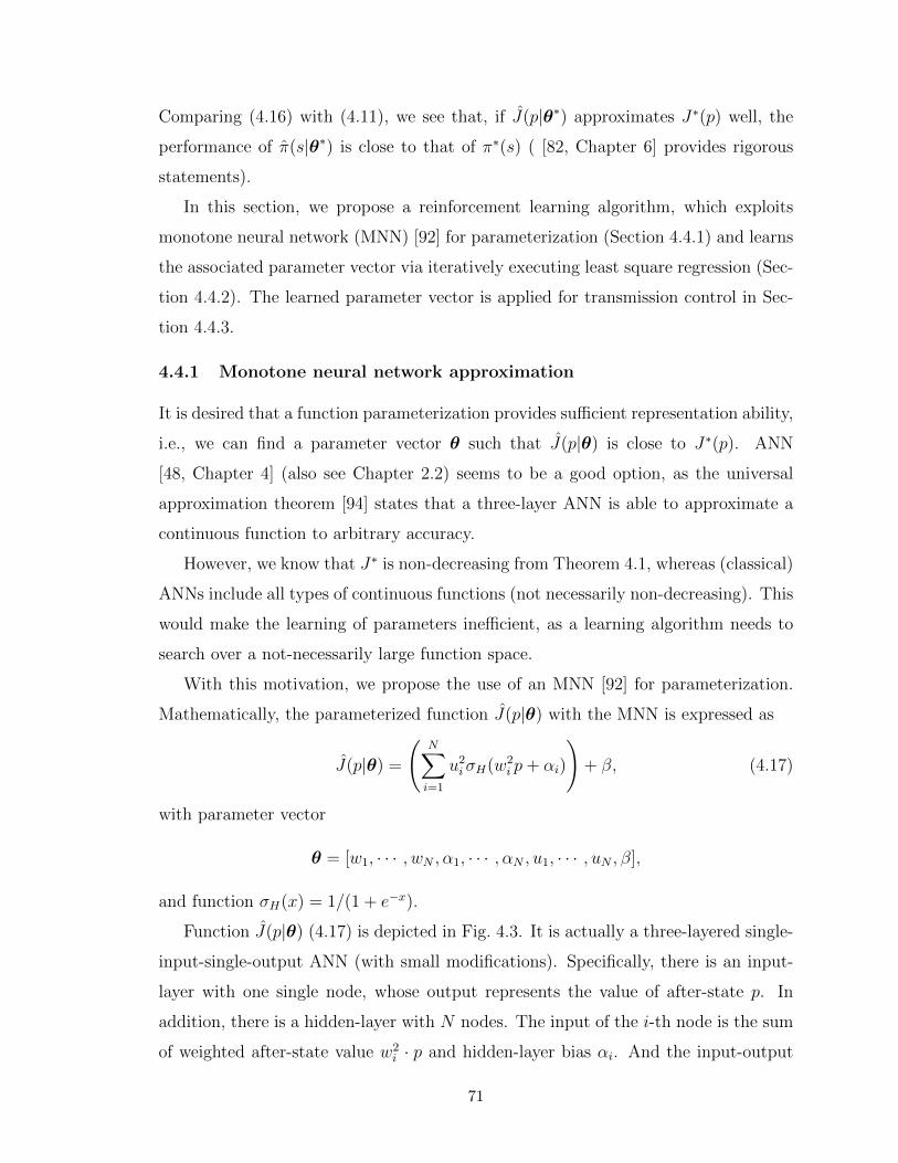
Comparing (4.16) with (4.11), we see that, if J(p|θ∗) approximates J∗(p) well, the

performance of π(s|θ∗) is close to that of π∗(s) ( [82, Chapter 6] provides rigorous

statements).

In this section, we propose a reinforcement learning algorithm, which exploits

monotone neural network (MNN) [92] for parameterization (Section 4.4.1) and learns

the associated parameter vector via iteratively executing least square regression (Sec-

tion 4.4.2). The learned parameter vector is applied for transmission control in Sec-

tion 4.4.3.

4.4.1 Monotone neural network approximation

It is desired that a function parameterization provides sufficient representation ability,

i.e., we can find a parameter vector θ such that J(p|θ) is close to J∗(p). ANN

[48, Chapter 4] (also see Chapter 2.2) seems to be a good option, as the universal

approximation theorem [94] states that a three-layer ANN is able to approximate a

continuous function to arbitrary accuracy.

However, we know that J∗ is non-decreasing from Theorem 4.1, whereas (classical)

ANNs include all types of continuous functions (not necessarily non-decreasing). This

would make the learning of parameters inefficient, as a learning algorithm needs to

search over a not-necessarily large function space.

With this motivation, we propose the use of an MNN [92] for parameterization.

Mathematically, the parameterized function J(p|θ) with the MNN is expressed as

J(p|θ) =

(N∑i=1

u2iσH(w2

i p+ αi)

)+ β, (4.17)

with parameter vector

θ = [w1, · · · , wN , α1, · · · , αN , u1, · · · , uN , β],

and function σH(x) = 1/(1 + e−x).

Function J(p|θ) (4.17) is depicted in Fig. 4.3. It is actually a three-layered single-

input-single-output ANN (with small modifications). Specifically, there is an input-

layer with one single node, whose output represents the value of after-state p. In

addition, there is a hidden-layer with N nodes. The input of the i-th node is the sum

of weighted after-state value w2i · p and hidden-layer bias αi. And the input-output

71

Hidden-layerInput-layer Output-layer

...

...

...

...

Figure 4.3: Monotone neural network

relationship of each hidden-layer node is defined by σH(·) (known as the sigmoid

activation function, see Chapter 2.2). Finally, there is an output-layer with one node,

whose output represents the ultimate approximated function value J(p|θ). Its input

is the summation of weighted outputs from the hidden-layer and the output-layer bias

β. And the output of the output-layer node is equal to its input.

Note that, the key difference between MNN and classical ANN is the sign of

weights. The MNN has non-negative weights, which is not necessary for classical

ANN. But MNN ensures J(p|θ) to be a non-decreasing function, which is proved in

Theorem 4.3.

Theorem 4.3. For any parameter θ, J(p|θ) is a differentiable non-decreasing func-

tion.

Proof. We have ddpJ(p|θ) =

∑Ni=1 u

2i ·w2

i ·σH(w2i p+αi) · (1−σH(w2

i p+αi)). It is easily

verified that ddpJ(p|θ) ≥ 0, which completes the proof.

In addition, Theorem 4.4 states that the proposed MNN has sufficient ability to

represent any continuous and non-decreasing function.

Theorem 4.4. For any continuous non-decreasing function J : [0, 1] 7→ R, there

exists an MNN with N hidden nodes and parameter vector θ, such that J(p)−J(p|θ) ≤

ε, for any p ∈ [0, 1] and ε ≥ 0.

Proof. It can be proven by [92, theorem 3.1], which considered a general case of

representing a multiple-input-single-output non-decreasing function.

72

Remark: Theorem 4.4 states that J(p|θ) is able to approximate J∗(p) to arbitrary

accuracy via optimizing the parameter vector θ.

4.4.2 Fitted value iteration to train MNN

Fitted value iteration [95] is a state-of-the-art learning methodology that is especially

useful for training neural networks for optimal control. When working with complex

neural networks (with multiple hidden layers), it is entitled with the name of deep

reinforcement learning [96, 97]. Here, we develop an algorithm, called FMNN (fitted

value iteration with monotone neural network), via tailoring the fitted value iteration

method into our problem. FMNN trains an MNN to approximate J∗(p) via exploiting

a batch of data samples. In the following, we first specify the required data. Then,

the training process is presented.

4.4.2.1 Collecting training data

The required training data for FMNN is a batch of samples F = (pm, sm = [bm, hm, dm])M−1m=0 ,

where bm ∼ fB(·|pm), hm ∼ fH(·) and dm ∼ fD(·). In the following, We provide two

possible methods for collecting F .

Suppose that there is a simulator that is able to generate data samples of random

variables ct, et, ht and dt that obey PDFs fC(·), fE(·), fH(·) and fD(·), respectively.

In this case, we can first obtain pmm by uniformly sampling over [0, 1]. Then,

for a given pm, we sample those random variables and get realizations (c, e, h, d).

With these realizations, a valid data sample (pm, sm) can be obtained by setting

sm = [((pm + e)− − c)+, h, d]. Finally, F is constructed by repeating the procedure

for all pm.

When such a simulator is not available, we can construct F via physically interact-

ing with environments. Specifically, we can run a certain sampling policy πS(s) (such

as the greedy policy, i.e., always choose to send if energy is sufficient). And during

the execution of πS(s), we can observe a sample path of random variables (..., st−1 =

[bt−1, ht−1, dt−1], pt−1 = %(st−1, πS(st−1)), st = [bt, ht, dt], pt = %(st, πS(st)), ...). Then,

by setting pm = pt−1 and sm = [bt, ht, dt], we are able to collect a valid sample

(pm, sm). Finally, F is constructed by sweeping from t = 0 to M .

73

4.4.2.2 Fitting MNN Iteratively

Here, we present FMNN, which trains an MNN to approximate J∗(p) with F via

imitating the iterative computing scheme of (4.13).

Specifically, similar to (4.13), FMNN works iteratively. At the kth iteration,

suppose that the current MNN parameter vector is θk, which defines a function

J(p|θk) with (4.17). As suggested by (4.13), given current value function Jk(p) =

J(p|θk), the updated value function should be

Jk+1(p) = γ · E[maxa

r(s′, a) + J(%(s′, a)|θk)

∣∣∣∣p] . (4.18)

Therefore, we wish to update the MNN’s parameters to obtain a new function J(p|θk+1)

that is close to Jk+1(p).

To do so, from F and θk, we construct a batch of data

Tk = (pm, om)M−1m=0 , (4.19)

where

om = γ ·maxa

r(sm, a) + J(%(sm, a)|θk)

. (4.20)

Note that by comparing (4.20) with (4.18), om can be seen as a noisy realization of

Jk+1(pm). In other words, given pm as an input value, om defines the corresponding

output of Jk+1 (plus certain noise). Therefore, we may get a function that is close

to Jk+1(p) by training the MNN to fit the (noisy) input-output patterns contained in

Tk.

Specifically, given Tk, the MNN parameter is updated as

θk+1 = arg minθL(θ|Tk) , (4.21)

where

L(θ|Tk) =1

2M

M−1∑m=0

(J(pm|θ)− om

)2

(4.22)

(the solving of (4.21) is discussed in Section 4.4.2.3). That is, the output of updated

function J(p|θk+1) minimizes the square error with respect to data set Tk, i.e., least

square regression. Given sufficiently large M , this regression process can efficiently

74

average out data’s randomness. Hence, the approximation error between Jk+1(p) and

J(p|θk+1) should be small.

With θk+1, we can generate Tk+1 from θk+1 and F (similar as (4.19)), and then

solve θk+2 by fitting the MNN to Tk+1 (similar as (4.21)). Iterations continue by

repeating the procedure. The ultimate learned function J(p|θK) after K iterations

should be close to J∗(p) with sufficiently large K. For illustration, Fig. 4.4 shows the

1st, 2nd and 20th iterations during FMNN’s execution. Summarizing above concepts,

FMNN algorithm is presented in Algorithm 4.1.

0 0.2 0.4 0.6 0.8 1

0

0.2

0.4

0.6

0.8

1

(a) The 1st iteration

0 0.2 0.4 0.6 0.8 1

0

0.2

0.4

0.6

0.8

1

1.2

1.4

(b) The 2nd iteration

0 0.2 0.4 0.6 0.8 1

0.5

1

1.5

2

2.5

3

(c) The 20th iterationFigure 4.4: Illustration of FMNN with |F| = 500

75

Algorithm 4.1 FMNN: Approximate J∗(p)

Require: Data samples F = (pm, sm)M−1m=0

Ensure: Learned MNN J(p|θK)1: procedure2: Randomly initialize parameter θ0

3: for k from 0 to K − 1 do4: for m from 0 to M − 1 do5: Get (pm, sm) as the mth element of F6: Compute om from θk and sm via (4.20)7: Collect Tk(m) = (pm, om)8: end for9: Regression: θk+1 = Fit(Tk,θk) (see Algorithm 4.2)

10: end for11: Learned MNN is determined from (4.17) with θ = θK12: end procedure

4.4.2.3 Train MNN with gradient descent

Here, we apply gradient descent to address (4.21) for solving MNN parameter θk+1

such that the represented function J(p|θk+1) fits an input-output pattern Tk in least

square error sense.

Gradient descent works by iteratively searching over the parameter space. Denote

θ(0) as the initial search point, which can be intuitively set as current MNN parameter

θk. By gradient descent, the parameter searching is conducted as follows

θ(l+1) = θ(l) − ξ(l) · ∇L(θ(l)), (4.23)

where ξ(l) is the updating step size and ∇L(θ(l)) is the gradient of L (4.22) at θ(l).

Given properly decreasing ξ(l) and sufficient number of iterations L, we set θk+1 =

θ(L), which is considered as an approximated solution of (4.21).

Lastly, we derive ∇L(θ). With Tk = (pm, om)M−1m=0 , the partial derivatives of L

76

can be obtained as follows

∂L∂β

=1

M

M−1∑m=0

εm, (4.24)

∂L∂ui

=1

M

M−1∑m=0

(εm · 2 · ui · σH(w2

i · pm + αi)), (4.25)

∂L∂αi

=1

M

M−1∑m=0

(εm · u2

i · σH(w2i · pm + αi)

×(1− σH(w2

i · pm + αi)) ), (4.26)

∂L∂wi

=1

M

M−1∑m=0

(εm · u2

i · σH(w2i · pm + αi)

×(1− σH(w2

i · pm + αi))· 2 · wi · pm

), (4.27)

where

εm = J(pm|θ)− om. (4.28)

Therefore, the gradient of of L is

∇L(θ) =[∂L∂w1

, · · · , ∂L∂wN

, ∂L∂α1

, · · · , ∂L∂αN

, ∂L∂u1, · · · , ∂L

∂uN, ∂L∂β

]. (4.29)

Summarizing above results, we provide Algorithm 4.2, which works as an inner

loop of FMNN for training an MNN to fit data set Tk.

Algorithm 4.2 Inner loop of FMNN: Fit input-output pattern

Require: Input-output pattern Tk, initial search point θkEnsure: Trained parameter θk+1

1: procedure2: θ(0) = θk3: for l from 0 to L− 1 do4: Compute ∇L(θ(l)) with Tk via (4.24)-(4.27)5: Obtain θ(l+1) with θ(l) and ∇L(θ(l)) via (4.23)6: end for7: θk+1 = θ(L)

8: end procedure

4.4.3 Apply learned MNN for transmission control

With the generated parameter θK , π(·|θK) is constructed from (4.16) by setting

θ∗ = θK . For large N , M and K, π(s|θK) (4.16) should be close to π∗(s) [98], and

can be applied for selective transmission control, which is presented in Algorithm 4.3.

77

Algorithm 4.3 Transmission control with learned MNN

Require: Learned MNN J(·|θK)1: procedure2: for t from 0 to ∞ do3: A packet arrives, and the node ends the silent period of cycle t4: Decode the packet and evaluate its priority dt5: Probe CSI and estimate required transmit energy ht6: Determine current remaining energy in battery bt7: Construct state st = [bt, ht, dt]8: Compute after-states p0 = %(st, 0) and p1 = %(st, 1)9: Evaluate after-state values with trained MNN as J0 = J(p0|θK) and J1 =J(p1|θK)

10: if J0 > J1 + 1(bt ≥ ht) · dt then . see (4.16)11: Discard the packet12: else13: Send the packet with energy ht14: end if15: Battery is replenished with harvested energy et16: Enter silent period of cycle t+ 117: end for18: end procedure

4.5 Numerical Simulation

We will next numerically study the learning characteristics of the proposed FMNN

and the performance of the learned policy. In Section 4.5.2, we investigate the learning

efficiency of FMNN. Section 4.5.3 demonstrates the performance of the learned policy.


We model the wireless channels as Rayleigh fading, which is the most common model

in wireless research. It is especially accurate for signal propagation in heavily built-

up urban environments. The channel power gain zt then has the PDF fZ(x) =

1µZe−x/µZ , x ≥ 0, where µZ presents the mean of zt.

We assume that energy is harvested from wind power, which is well characterized

by the Weibull distribution [80]. Hence, we model et with Weibull PDF fE(x) =

kEλE

(xλE

)kE−1

e−(xλE

)kE−1

, x ≥ 0, with shape parameter kE = 1.2 and scale parameter

λE = 0.15/Γ(1 + 1/kE), where Γ(·) denotes the gamma function and µE represents

the mean of et.

Moreover, the total energy consumption ct during the silent period, data reception,

78

and channel estimation is modeled as a Gamma PDF fC(x) =(

Γ(kC)θkCC

)−1

xkC−1e− xθC , x >

0, with shape parameter kC = 10, and scale parameter θC = 0.02/kC . The combina-

tion of shape and scale parameters implies that the mean of ct equals 0.02.

Furthermore, the model of data priority dt depends on the specific practical ap-

plication. We assume that dt is exponentially distributed, i.e., fD(d) = e−d, d ≥ 0,

which is also considered in [85,90]. This assumption is sensible, since for many appli-

cations, such as system monitoring, where high-priority packets that indicate critical

events should happen with small probability, while the most of packets should have

low priorities.

Finally, the number of hidden nodes N of the MNN is set to 3. The FMNN is

executed with the data sample size of |F| = M = 500, and the number of iterations

K = 20.

4.5.2 Sample efficiency for learning π∗

To evaluate learning efficiency of FMNN, we use the sample efficiency, which eval-

uates the amount of data samples needed to be processed before an algorithm can

learn a (near) optimal policy. Sample efficiency is a good proxy of an algorithm’s

training ability and adaptivity. We next assess the sample efficiency of FMNN and

that of two alternatives, namely FNN (fitted value iteration with classical neural net-

work) and Online-DIS (online learning with after-state space discretization), which

are constructed as follows.

4.5.2.1 FNN and Online-DIS

FNN is the same as FMNN except replacing the MNN as a three-layer classical ANN

(without non-negative weights constraint) and modifying the gradient descent method

for ANN in Algorithm 4.2. Thus, FNN does not exploit the monotonicity of J∗, and

the learning efficiency is expected to be inferior to that of FMNN.

Online-DIS algorithm is developed via applying the well-known Q-learning algo-

rithm [50, Chapter 6.5] into our problem (Q-learning is also chosen for comparison

in [90]). Online-DIS applies discretization for parameterization and an online learn-

ing scheme for learning associated parameters. Specifically, Online-DIS discretizes

the after-state space into N bins, which are, respectively, associated with N param-

79

eters. The nth parameter presents the “aggregated” function values of J∗(p) for all

after-states p that fall into the nth bin. These parameters are learned via continu-

ously updating parameters with each available sample. In order to properly average

out data samples’ randomness, the updating step size needs to be sufficiently small

(see [50, p. 39]). Therefore, the learning generally progresses fairly slowly, and requires

a large amount of data samples.

4.5.2.2 Sample efficiency comparison

The setting of FNN is the same as that of FMNN. For Online-DIS, the number of bins

N is set as 20. To investigate the learning efficiency, we evaluate the performance

of learned policies after consuming certain amount of data samples. The results are

shown in Fig. 4.5 with logarithmic scale. Note that each iteration of FMNN and FNN

consumes 500 data samples, and Fig. 4.5 shows the learning progress for the first 20

iterations.

5e2 1e3 1e4 1e5 1e6

Consumed data samples

0.06

0.08

0.1

0.12

0.14

0.16

0.18

Av

erag

ed r

ewar

ds

Online-DIS

FNN

FMNN

5 10

105

0.16

0.18

Figure 4.5: Learning curve

Firstly, we observe that FMNN and FNN are about 100 times more efficient than

Online-DIS. This significant disparity occurs because FMNN and FNN directly train

an MNN/ANN to fit data samples with regression, whereas Online-DIS must gradu-

ally average out randomness with a small step size.

Secondly, FMNN learns considerably faster than FNN. Because FMNN exploits

80

the non-decreasing property of J∗, it can learn a reasonably good policy with fewer

iterations.

Finally, after processing enough data samples, all three learning curves converge.

Both FMNN and FNN converge to the same value, while Online-DIS converges to a

slightly inferior level. The reason is that both FMNN and FNN are able to represent

a continuous non-decreasing function. Therefore, their learned policies achieve the

same performance. However, the function represented by Online-DIS is piece-wise

constant (see Fig. 4.6 below), and the discontinuity causes certain performance loss.

0 0.2 0.4 0.6 0.8 10.6

0.8

1

1.2

1.4

1.6

1.8Online-DIS

FNN

FMNN

(a) FMNN and FNN after 1.5× 103 samples, andOnline-DIS after 1.5× 105 samples

0 0.2 0.4 0.6 0.8 11

1.2

1.4

1.6

1.8

2

Online-DIS

FNN

FMNN

(b) FMNN and FNN after 104 samples, andOnline-DIS after 106 samples

Figure 4.6: Learned value functions

The above analysis is confirmed in Fig. 4.6. Fig. 4.6(a) shows that, after processing

1.5× 103 samples (3 iterations), FMNN learns a good value function, which is fairly

close to the function learned after consuming 104 samples (20 iterations) as shown

in Fig. 4.6(b). The function learned by FNN after processing 1.5× 103 samples does

not capture the non-decreasing structure of J∗. This fact suggests FNN’s inferior

sample efficiency compared with FMNN. Nevertheless, its ultimate learned function

converges to that of FMNN, which provides the same limiting performance as achieved

by FMNN. Finally, as one can notice, with 1.5×105 data samples, the function learned

by Online-DIS is fluctuated, since the randomness of data samples has not be averaged

out. Given 106 data samples and gradually decreasing step size, Online-DIS properly

averages out noise and learns a non-decreasing function to fit J∗. However, due to the

nature of after-state space discretization, the learned function is piece-wisely constant,

81

whose discontinuity causes slight performance loss of the resulted policy.

4.5.3 Achieved performance of learned policy

Given FMNN’s learned parameter θK , the policy π(s|θK) defined with (4.16) can then

be applied for selective transmission control via Algorithm 4.3. The major difference

between the developed policy π(s|θK) and polices proposed in existing works [85–90]

is that: polices of [85–90] make decisions based on available energy bt and packet

priority dt, whereas π(s|θK) further exploits CSI ht. To investigate the performance

gain of exploiting CSI, we compare π(s|θK), named as DecBDH (i.e., decision based

on bt, dt, and ht), with the policy of work [90], named as DecBD (i.e., decision based

on bt and dt). Note that works [85–89] do not fit energy-harvesting and/or wireless

fading settings. DecBD works as follows. It first follows the scheme in [90] to decide

whether or not to send based on available energy bt and packet priority dt. When

“to send” is chosen, the node transmits with energy ht if bt ≥ ht, or drops the packet

without energy consumption otherwise.

We also compare with an adaptive transmission (AdaTx) scheme, which always

tries to send if a successful transmission can be achieved, i.e., the node transmits with

energy ht if bt ≥ ht, or drops the packet without energy consumption otherwise.

1 1.5 2 2.5 3 3.5 40.2

0.3

0.4

0.5

0.6

Av

erag

ed r

ewar

ds

DecBDH

DecBD

AdaTx

Figure 4.7: Achieved performance under different channel conditions

With µE = 0.15, Fig. 4.7 shows the performance of DecBDH, DecBD and AdaTx

under different channel conditions. As one can see, DecBD outperforms AdaTx. The

82

reason is that, via jointly considering dt and bt, DecBD is able to put more attention

on high priority packets and avoid transmission when available energy level is low.

Exploiting instantaneous CSI, DecBDH makes transmission decisions based on the

channel status as well as the available energy and data priority, which enables it to

obtain more transmission opportunities at good channel conditions, and therefore,

achieve higher performance than DecBD.

4.6 Summary

In this chapter, we investigated the transmission policy of an energy-harvesting sensor,

where low-priority packets can be dropped for transmitting more important packets

over in a long term. Based on after-state value function, we constructed the optimal

selective transmission policy, which decides whether or not to send each packet based

on the sensor’s battery level, the packet’s priority and channel status. Then, the policy

is further proved to be threshold-based with respect to data priority and channel

status. Finally, exploiting the discovered structure, we proposed to learn the optimal

policy with monotone neural network, which demonstrates high sample efficiency.

4.7 Appendix

4.7.1 Proof of Lemma 4.1

Since bt+1 = ((pt + et)− − ct+1)+, we have, for x ∈ [0, 1],

Prob(bt+1 > x|pt = p) = Prob(((p+ et)− − ct+1)+ > x)

= Prob((p+ et)− > x+ ct+1)

= Prob(1 > x+ ct+1 and p+ et > x+ ct+1)

=

∫ 1−x

0

∫ 1

x−pfE(e) · fC(c) de dc, (4.30)

where Prob(·) means probability, and the last equality holds as et has PDF fE and

ct+1 has PDF fC .

It is easy to check that Prob(bt+1 > x|pt = p) does not depend on t, and

FB(b|p) = 1− Prob(bt+1 > b|pt = p). (4.31)

83

In addition, since fE and fC are both non-negative, Prob(bt+1 > b|pt = p) (4.30) is

non-decreasing with respect to p, which implies FB(t|p) is non-increasing with respect

to p from (4.31). Finally, it is obvious that ddpFB(t|p) and d

dtFB(t|p) exist (and can be

computed via the Leibniz integral rule), which completes the proof.


With value iteration algorithm (4.13), we prove Theorem 4.1 by induction. Specifi-

cally, we set J0(p) = 0 for all p ∈ [0, 1], which is differential and non-decreasing. With

this choice of J0, we can prove Theorem 4.1 by showing that, if Jk is non-decreasing

and differentiable, Jk+1 is non-decreasing and differentiable.

First, from (4.13), we have

Jk+1(p) = γE[r(s′, A′) + Jk(%(s′, A′))

∣∣p], (4.32)

where the expectation is taken over both s′ and A′, and A′ is a function of random

variable s′:

A′ =

1 if r(s′, 1) + Jk(%(s′, 1)) ≥ Jk(%(s′, 0))

0 otherwise.

In addition, due to the induction assumption and the fact %(s′, 1) ≤ %(s′, 0), we

have Jk(%(s′, 1)) ≤ Jk(%(s′, 0)). Therefore, if A′ = 1, we must have b′ ≥ h′, since

b′ < h′ implies r(s′, 1) = 0, and further implies r(s′, 1) + Jk(%(s′, 1)) < Jk(%(s′, 0)),

and therefore, A′ = 0 (a contradiction of A′ = 1).

Denoting Si(b) as the region of (h, d) where action A′ = i ∈ 0, 1 given b, we have

S1(b) = (h, d)|b ≥ h, d+Jk(b−h) > Jk(b), and S0(b) = (h, d)|b ≥ h, d+Jk(b−h) ≤

Jk(b) ∪ (h, d)|b < h. Given S0(b) and S1(b), Jk+1(p) (4.32) can be rewritten as

Jk+1(p) = γ

∫ 1

0

fB(η|p) ·M(η) dη, (4.33)

where

M(η) ,∫∫

(x,y)∈S1(η)

[y + Jk(η − x)

]· fD(y) · fH(x) dy dx

+

∫∫(x,y)∈S0(η)

Jk(η) · fD(y) · fH(x) dy dx

=

∫ η

0

∫ +∞

Jk(η−x)

(y + Jk(η − x)

)· fH(x) · fD(y) dy dx

84

+

∫ η

0

∫ Jk(η−x)

0

Jk(η) · fH(x) · fD(y) dy dx

+

∫ +∞

t

∫ +∞

0

Jk(η) · fH(x) · fD(y) dy dx. (4.34)

In the following, we present Lemma 4.2, whose proof is given in Section 4.7.3.

With Lemma 4.2 and (4.33), we thereby can complete the proof by showing that

M(η) is differentiable and non-decreasing.

Lemma 4.2. Given that function Ω(η) is non-decreasing and differentiable for η ∈

[0, 1], function J(p) generated with J(p) =∫ 1

η=0fB(η|p)Ω(η) dη is non-decreasing and

differentiable for p ∈ [0, 1].

With the assumption that Jk(p) is differentiable, the function M(η) can be shown

to be differentiable by repeatedly using the Leibniz’s rule. Therefore, we are remaining

to show that M(η) is non-decreasing.

Given any η1, η2 ∈ [0, 1] and η1 ≥ η2, we define Sij , Si(η1) ∩ Sj(η2) with i, j ∈

0, 1. Then, from (4.34), it is easy to verify that

M(η1)−M(η2) = E[1((h, d) ∈ S11) ·

(Jk(η1 − h)− Jk(η2 − h)

)]︸︷︷︸,∆11

+ E[1((h, d) ∈ S10) ·

(d+ Jk(η1 − h)− Jk(η2)

)]︸︷︷︸,∆10

+ E[1((h, d) ∈ S01) ·

(Jk(η1)− d− Jk(η2 − h)

)]︸︷︷︸,∆01

+ E[1((h, d) ∈ S00) ·

(Jk(η1)− Jk(η2)

)]︸︷︷︸,∆00

,

where the expectations are taken over h and d. With the assumption that Jk(p) is non-

decreasing, the following results hold. Since η1 ≥ η2, we have Jk(η1−H) ≥ Jk(η2−H)

and Jk(η1) ≥ Jk(η2), and therefore, ∆11 ≥ 0 and ∆00 ≥ 0. And according to the

definition of S10, we have dt + Jk(η1 −H) ≥ Jk(η1) ≥ Jk(η2), which means ∆10 ≥ 0.

Finally, for S01, we have Jk(η1) ≥ dt + Jk(η1 − H) ≥ dt + Jk(η2 − H), which means

∆01 ≥ 0. In summary, we have M(η1) −M(η2) ≥ 0 given η1 ≥ η2. Therefore, M(η)

is non-decreasing.

85

4.7.3 Proof of Lemma 4.2

Suppose the derivative of Ω(η) in η ∈ [0, 1] is ω(η). Since Ω(η) is non-decreasing, we

have ω(η) ≥ 0. Then, using integration by parts, we have

J(p) = Ω(1)− Ω(0)FB(0|p)−∫ 1

0

ω(η) · FB(η|p) dη, (4.35)

where the fact FB(1|p) = 1 is exploited. From Lemma 4.1, FB(η|p) is non-increasing

respected to p for any η. This means that −Ω(0)FB(0|p) is non-decreasing. Further-

more, because ω(η) ≥ 0, we have −∫ 1

0ω(η) · FB(η|p) dη is non-decreasing (respected

to p). In summary, J(p) is non-decreasing.

In addition, since FB(η|p) is differentiable over p, it is easy to see from (4.35) that

J(p) is differentiable over p.

86

Chapter 5

Cooperative Spectrum Sensingunder Heterogeneous SpectrumAvailability

5.1 Introduction

Sensing spectrum for correctly detecting PUs is crucial for cognitive radio systems,

since it maximizes transmission opportunities, and also limits SUs’ interference to

PUs. However, due to channel propagation impairments, especially wireless fading, it

is difficult for an SU to achieve reliable detection via independently sensing spectrum.

Fortunately, the sensing reliability can be improved by fusing spectrum measurements

from multiple, spatially-separate secondary nodes, known as cooperative spectrum

sensing (CSS).

Most of existing works on CSS (see [23] and references therein) assumed a spectrum

homogeneity setting, i.e., all cooperating SUs observe the same PU and experience

the same spectrum availability status. This assumption is reasonable for PUs with

large transmission power, such as television broadcast systems [15], and/or small-

scale secondary networks where all SUs are co-located. However, in other cases (e.g.,

secondary networks with large geographical expansion), some SUs may be too close

to PUs, and therefore, experience the busy spectrum status (i.e., do not allowed to

transmit), while the other SUs are far away from PUs, and therefore, experience

the free spectrum status. That is, SUs at different spatial locations may experience

different spectrum availability statuses, i.e., a heterogeneous spectrum availability

setting.

87

Considering sensing tasks in presence of heterogeneous spectrum availability, we

take the view point of distance. That is, an SU is allowed to transmit, if it is certain

distance far away from active PUs [99]. Such a distance, named as protection range

(PrR), can be rigorously computed via considering PU interference tolerance, PU

and SU transmission power and others [100, 101]. Therefore, for an SU, the goal of

spectrum sensing is to decide whether it is within the PrR of any active PU.

Despite heterogeneous spectrum availability, sensing cooperation is still benefi-

cial. It is because spatially proximate SUs are likely to fall within the PrR of the

same PU, and therefore share the same spectrum status. Hence, spatial informa-

tion is a key for applying CSS. We do not exploit SU location information, as it can

be hard to obtain. Instead, SU neighbor information is assumed: we assume that

each SU knows its neighboring SUs, i.e., SUs within the SU’s transmission range.

Therefore, the problem is, under heterogeneous spectrum availability, how

to exploit neighbor information to fuse SU observations for improving

sensing performance.

As the easiest way, work [102] showed that, in presence of heterogeneous spectrum

availability, an SU can improve sensing performance via combining individual hard

decisions of its neighbors. However, since strong spectrum correlation may exist

between SUs over several hops, it is important to consider sensing cooperation beyond

one hop.

To do so, works [103–106] applied (pairwise) Markov random fields (MRFs)

[107] (also see Chapter 2.3) to model the prior distribution of SUs’ spectrum statuses.

MRFs exploit a Markovian approximation: the spectrum status of an SU is indepen-

dent of those of non-adjacent SUs, given its adjacent SUs’ spectrum statuses. MRFs

heuristically build up the prior distribution via capturing the strongest spectrum

correlations among SUs.

With prior distribution, works [103–106] attempted to infer spectrum statuses via

marginalization. Specifically, combining MRF prior with sensing observations (which

specify data likelihood functions), a posterior distribution over all SUs’ spectrum

statuses can be obtained. Then, the sensing decision of an SU is made based on the

marginal distribution of the SU’s spectrum status, which can be computed from the

posterior distribution via summing over the spectrum statuses of all other SUs. Due to

88

the curse of dimensionality, exactly computing the marginal distribution is impractical

in large-scale secondary networks. Fortunately, thanks to MRFs’ simple structure,

an approximated version of the marginal distribution can be computed via belief

propagation (BP) algorithms [108, Chapter 11], where SUs distributedly estimate

their corresponding marginal distributions via iteratively exchanging messages with

their neighbors.

5.1.1 Motivations

Approximately computing marginal distributions via BP algorithms, as considered

in [103–106], provides a useful methodology to fuse SUs’ sensing observations for

decision making. However, there are two theoretical and one practical downsides for

this methodology.

Theoretically, BP algorithms do not have convergence guarantee. In addition,

when convergence is reached, the computed distribution does not equal the true

marginal distribution [108, p. 392]. Practically and more importantly, BP algorithms

best fit distributed networks with low SU density, but may not work well in other

networks. The reason is that BP algorithms’ major computation advantage comes

from parallelization. This benefit vanishes in centralized secondary networks, where

sensing information and decisions need to be processed in central infrastructures.

Moreover, the computation complexity for an SU to execute BP algorithms is expo-

nential in the number of its neighbors. Hence, it is computationally demanding to

apply BP algorithms in secondary networks with high density.

5.1.2 Contributions

To address the above limitations, we propose a different methodology. Specifically, we

still use MRFs for modeling the prior distribution, but we infer spectrum statuses via

solving the maximum a posterior (MAP) problem (instead of marginal distributions).

Roughly speaking, sensing decisions are jointly made by solving the configuration of

SU spectrum statuses that maximizes the posterior distribution, which is named an

MAP-MRF problem.

Note that, similar to marginalization, MAP-MRF is a meaningful formulation for

inferring spectrum statuses from sensing observations. More importantly, thanks to

89

optimization theory, the MAP-MRF problem can be solved more efficiently and flex-

ibly than marginalization. Based on MAP-MRF, we propose three CSS algorithms,

which are, respectively, designed for centralized, cluster-based and fully distributed

secondary networks.

For centralized secondary networks, we propose a CSS algorithm based on graph

cut theory, named as GC-CSS. GC-CSS exactly solves the MAP-MRF problem with

polynomial time complexity in both network size and density.

For cluster-based secondary networks (where sensing information and decision of

each cluster are processed centrally), we develop a CSS algorithm based on dual de-

composition theory, named as DD-CSS. DD-CSS is able to obtain sensing decisions

distributedly (at cluster-level) via iteratively exchanging (binary) messages among

clusters.

For distributed secondary networks, we obtain a CSS algorithm, named as DD1-

CSS, which is a special case of DD-CSS, when each SU forms a cluster. DD1-CSS

works similar to BP algorithms via exchanging messages among SUs. However, com-

pared with BP algorithms, DD1-CSS has following advantages. First, DD1-CSS has

theoretical guarantee (for solving the MAP-MRF problem). In addition, each SU’s

computation complexity is polynomial in the number of its neighbors. Finally, its

communication overhead is low.

The rest of this chapter is organized as follows. In Section 5.2, the system model

is presented. The CSS problem based on MAP-MRF is formulated in Section 5.3.

GC-CSS, DD-CSS, DD1-CSS algorithms are proposed in Sections 5.4, 5.5 and 5.6,

respectively. Section 5.7 demonstrates several numerical simulation results.

Notation conventions: Most of the notations in the rest of this Chapter fol-

low the conventions below (exceptions can be easily understood from context): 1) a

lowercase letter x denotes a scale variable or a random variable’s realization; 2) a

capitalized letter X denotes a random variable; 3) a hatted variable x denotes an es-

timation of x; 4) a bold variable x denotes a vector; 5) a calligraphy letter X denotes

a set.

90

5.2 System Model

5.2.1 Network setup

We consider a disc with radius R (see Fig. 5.1), which represents the area of interest.

There are N SUs randomly and uniformly located within the disc, and these SUs do

not move. It is assumed that SUs are unaware of their own locations. The N SUs

are indexed as SU1, ..., SUN .

Figure 5.1: Network setup

At each sensing period, a PU appears randomly within the disc, and transmits

signal. Let r denote PrR and di denote the distance between SUi and the PU.

Therefore, SUi’s spectrum status is “busy”, denoted as xi = 1, if 0 ≤ di ≤ r; and

SUi’s spectrum status is “free”, denoted as xi = 0, if r < di ≤ R. It is easy to see

that SUs at different locations may have different spectrum statuses, a heterogeneous

spectrum availability setting.

5.2.2 Signal model and data likelihood functions

SUi measures the energy of received primary signal, denoted as yi, in order to infer its

spectrum status xi. Intuitively, if the measured energy yi is small, SUi is likely to be

far away from the PU, and therefore, xi is likely to be 0, and vice versa. In following,

we mathematically model the relationship between (observed) energy measurement

yi and (unobserved) spectrum status Xi.

Assume that the primary signal received by SUs experiences static path loss and

Rician fading. Therefore, the complex channel gain between the PU and SUi, denoted

91

as Hi, is modeled as

Hi = (1 +Di)−α/2Ψi,

where α > 0 is the propagation factor, and Ψi denotes the complex gain of a Rician

fading channel. Note that, the distance Di is treated as a random variable, since the

locations of SUs and the PU are unknown. We assume that Ψii are independent

and identically distributed, and do not change during a sensing period, i.e., a block

fading assumption. Therefore, givenM signal samples, the measured energy Yi (before

observation) can be expressed as

Yi =M∑m=1

|HiS(m) +W (m)|2,

where S(m), representing the mth sample of primary signal, is modeled as a random

variable that obeys CN (0, 2σ2S) (zero-mean complex normal distribution with variance

2σ2S), and W (m), representing the mth sample of background noise, is modeled as a

random variable that obeys CN (0, 2σ2W ).

It is known that |Ψi|2 follows a noncentral chi-square distribution. Without loss

of generality, the PDF of |Ψi|2 can be expressed as

f|Ψ|2(|ψi|2) = 2(kH + 1) |ψi|2 exp(−(kH + 1)|ψi|4 − kH

)× I0

(2√kH(kH + 1)|ψi|2

), (5.1)

where kH (known as the K-factor) accounts for the power ratio between the line-of-

light path and scattered paths, and I0(·) is the zeroth order modified bessel function

of the first kind. Note that, f|Ψ|2(·) does not depend on i, since Ψii are assumed to

be independent and identically distributed.

In addition, from [54], the PDF of Yi given Di and |Ψi|2 is

fY |D,|Ψ|2(yi | di, |ψi|2) =yM−1i exp(− yi

2(1+ξi)σ2W

)

(2(1 + ξi)σ2W )MΓ(M)

(5.2)

where Γ(·) is the gamma function and ξi = (1 + di)−α|ψi|2σ2

S/σ2W . Note that,

fY |D,|Ψ|2(·|·, ·) does not depend on i, since, given Di = di and |Ψi|2 = |ψi|2, Yi’s

randomness only stems from the primary signal and background noise.

92

Finally, we (approximately) model the PDF of Di given Xi as

fD|X(di | xi = 0) =

2di/(R

2 − r2) if di ∈ (r, R],

0 otherwise,(5.3a)

fD|X(di | xi = 1) =

2di/r

2 if di ∈ [0, r],

0 otherwise.(5.3b)

Note that fD|X(di | xi) exactly matches the network setup of Section 5.2.1 only if SUi

is located at the center of the disc. However, since SUs are unaware of their locations,

it is reasonable to apply fD|X(· | ·) to SUi for all i.

Based on (5.1), (5.2), (5.3), we can obtain the PDF of Yi given Xi as

fY |X(yi | xi) =

∫ ∞|ψi|2=0

∫ R

di=0

fY |D,|Ψ|2(yi | di, |ψi|2

)fD|X (di | xi) f|Ψ|2

(|ψi|2

)ddi d|ψi|2.

(5.4)

Given observed energy measurement yi, fY |X(yi | xi), known as data likelihood func-

tion, represents the likelihood that Xi = xi. Therefore, SUi can apply individual

spectrum sensing (Ind-SS) to infer its spectrum status. That is, SUi makes sensing

decision as

xi =

1 if γ fY |X(yi | 1) > fY |X(yi | 0),

0 otherwise,(5.5)

where weight γ > 0 is used to balance detection probability with false alarm prob-

ability. However, Ind-SS can be unreliable, especially when kH is small (i.e., poor

channel conditions). In Section 5.3, we exploit an MRF model to improve sensing

reliability via fusing sensing data from other SUs.

Note: In this chapter, we consider a single PU case for simplicity. Our sub-

sequently proposed MAP-MRF formulation (Section 5.3) and CSS algorithms (Sec-

tions 5.4-5.6) apply to more general settings, as long as a data likelihood function

similar to (5.4) can be obtained for corresponding environments.

5.3 CSS with MAP-MRF Formulation

Despite the heterogeneous spectrum availability setting (section 5.2.1), proximately

located SUs are likely to experience the same spectrum status. Therefore, we would

like to exploit this intuition to improve sensing performance via properly fusing sens-

ing data. For this purpose, we next construct an MRF, and then present the MAP-

MRF methodology for CSS.

93

5.3.1 Define SU-graph and MRF

It is assumed that, upon network’s setup, each SU performs neighbor discovering, from

which the SU knows its neighbors (SUs within its transmission distance). With this

neighbor information, we define an SU-graph, which is an undirected graph, denoted

as G = (V , E) with V and E representing the set of nodes and edges, respectively. For

the node set, we have V = 1, · · · , N, where node i represents SUi. The edge set E

is defined as

E = (i, j)| SUi and SUj are neighbors. (5.6)

Note that, since edges of G are undirected, (i, j) and (j, i) are the same element of E .

Here, we apply an MRF over SU-graph G to model the prior distribution of X ,

[X1, · · · , XN ]. MRF exploits an Markovian approximation: the spectrum status of

an SU is independent of those of non-adjacent SUs, if its adjacent SUs’ spectrum

statuses are known. Specifically, the prior belief (before observing sensing data) that

X = x , [x1, · · · , xN ] is modeled as

ΦX(x) =1

B

∏(i,j)∈E

φ(xi, xj), (5.7)

where B is a constant for normalization, E is defined in (5.6), and φ(xi, xj), named

as the potential function, is defined as

φ(xi, xj) = exp (β (xixj + (1− xi)(1− xj))) , (5.8)

where β > 0 is the hyperparameter of the MRF model. Note that, for the potential

function, we have φ(0, 0) = φ(1, 1) = exp(β) > φ(0, 1) = φ(1, 0) = 1, which repre-

sents the correlation between adjacent SUs, and the hyperparameter β controls the

correlation strength. We assume that β has been chosen properly (see Section 5.7.2

for choosing β).

5.3.2 Fuse data over MRF

5.3.2.1 Existing scheme based on marginalization

Given the MRF prior and sensing data y , [y1, · · · , yN ], works [103–106] considered

marginalization for CSS. Specifically, from (5.4) and (5.7), a posterior distribution of

94

X given y is first obtained

pX(X = x|y) = ΦX(x)∏i∈V

fY |X(yi | xi). (5.9)

Then, to decide the spectrum status of an SU, say SUi, works [103–106] attempt to

estimate the marginal (posterior) distribution of Xi

pXi(Xi = xi | y) =∑x1

· · ·∑xi−1

∑xi+1

· · ·∑xN

pX ([x1, · · · , xi−1, xi, xi+1, · · · , xN ]|y)

,∑

x′:x\xi

pX(x′ | y), (5.10)

where∑x′:x\xi[·] means to “marginalize over all variables within x except xi”, which

is introduced for notation convenience. Note that pXi(xi | y) represents the probabil-

ity that Xi = xi by jointly considering the spatial correlation ΦX(x) and sensing data

y. Therefore, given an estimated pXi(xi | y), SUi decides xi = 1 if pXi(1 | y) ≥ T

(T ∈ (0, 1) is a threshold), and decides xi = 0 otherwise. See Section 5.6.2.1 for how

to compute pXi(xi | y) via BP algorithms.

5.3.2.2 Proposed scheme based on maximization

Instead of following above methodology, we consider the (weighted) MAP estimation

of x. Specifically, given ΦX(x) and y, we solve xMAP = [xMAP1 , · · · , xMAP

N ] such that

xMAP = arg maxx

∏(i,j)∈E

φ(xi, xj)∏i∈V

γxifY |X(yi|xi)

, (5.11)

where weight γ > 0 (similar to T ) introduces trade off between detection probability

and false alarm probability. It can be seen that xMAP is the most probable configu-

ration of x given spatial correlation ΦX(x) and sensing data y. In other words, via

deciding SUs’ spectrum statuses x , [x1, · · · , xN ] = xMAP, we maximize the ‘like-

lihood’ of correctly determining SUs’ spectrum statuses, based on MRF prior and

sensing observations. Note that, when there is no spatial correlation among SUs, i.e.,

β = 0, the above decision making scheme reduces to Ind-SS (5.5).

Remark: Both (5.10) and (5.11) are meaningful sensing decision making schemes

that effectively fuse data via the MRF model. It is not important to determine which

one is a more theoretically proper formulation, since the MRF model is merely an

95

approximation of SUs’ actually spatial correlation. The key point is that, (5.11)

can be solved more efficiently and flexibly than (5.10), which will be discussed in

Sections 5.4, 5.5 and 5.6.

5.3.2.3 Transform to posterior energy

For the convenience of CSS algorithms’ development in subsequence sections, we

define a function, called posterior energy, for any x as

E(x) = − ln

∏(i,j)∈E

φ(xi, xj)∏i∈V

γxifY |X(yi|xi)

=∑

(i,j)∈E

κ(xi, xj) +∑i∈V

ηi(xi),

(5.12)

where κ(xi, xj), called the edge energy, is defined as

κ(xi, xj) = − ln(φ(xi, xj)) = −β (xixj + (1− xi)(1− xj)) (5.13)

and ηi(xi), called the unitary energy, is defined as

ηi(xi) = − ln(γxifY |X(yi|xi)). (5.14)

It is easy to see that we have

xMAP = arg minxE(x) , (5.15)

which is named as the MAP-MRF problem. In following sections, we will develop

three CSS algorithms for (approximately) solving xMAP.

5.4 GC-CSS for Centralized Secondary Networks

This section presents GC-CSS, which is designed for centralized secondary networks.

Assuming SU neighbor information and sensing information (provided by a central

infrastructure), the CSS decision xMAP is obtained by solving a so-called min-cut

problem. Note that MAP-MRF problems are first formulated as min-cut problems

in [109] for image segmentation task. Compared with [109], we provide a different

formulation and proof.

96

5.4.1 BF-graph and min-cut

In this subsection, we define a BF-graph and its associated min-cut problem. BF-

graph is an undirected graph with weighted edges, denoted as GBF = (VBF , EBF , c(·)),

with VBF , EBF , and c(·), respectively, represent node set, edge set and cost function

associated with edges.

The node set and edge set are constructed from SU-graph G as follows. We define

node set VBF = V ∪ b, f, where b and f are two nodes representing the busy and

free spectrum statuses, respectively. See Fig. 5.3 for an example of BF-graph, which

is constructed from the SU-graph of Fig. 5.2.

We define edge set EBF = E ∪ (b, i)i∈V ∪ (f, i)i∈V . That is, EBF consists of 3

types of edges: E , (b, i)i∈V and (f, i)i∈V (which are respectively, represented as

black, orange and blue lines in Fig. 5.3).

Edge cost function c(·) is specified for the 3 types of edges as follows. We assign

cost for edge (i, j) ∈ E as

c(i, j) = β, (5.16)

assign cost for edge (b, i), ∀i, as

c(b, i) = ηi(0) +Mi, (5.17)

assign cost for edge (f, i), ∀i, as

c(f, i) = ηi(1) +Mi, (5.18)

where ηi(0) and ηi(1) are defined in (5.14), and Mi is a constant ensuring both c(b, i)

and c(f, i) are nonnegative. For example, we can define Mi = ln (γf(yi|1) + f(yi|0)).

Figure 5.2: An example of SU-graph

A cut K = (B,F) of the BF-graph is a bipartition of VBF such that B ∩ F = ∅,

B∪F = VBF , b ∈ B and f ∈ F . The cut-set of K is EK = (i, j) ∈ EBF |i ∈ B, j ∈ F.

97

Figure 5.3: BF-graph and graph cuts

It can be seen that, after removing edges of EK , node b is separated from node f in

graph GBF . The cost c(K) of a cut K is defined as the summation of the cost of all

edges within EK , i.e.,

c(K) =∑e∈EK

c(e).

In the example of Fig. 5.3, (B = b, 5, 6, 7,F = f, 1, 2, 3, 4) defines a cut, whose

cost is∑4

i=1 c(f, i) +∑7

i=5 c(b, i) + 3β.

Denote K as all possible cuts. The min-cut K∗ is the cut that attains the minimum

cost among K, i.e.,

K∗ = arg minK∈K

c(K). (5.19)

Problem (5.19) can be solved efficiently, as stated in Theorem. 5.1, which is proved

in [110, Chapter 26].

Theorem 5.1. For an SU-graph with N nodes and |E| edges, problem (5.19) can be

solved (via Ford-Fulkerson algorithm [111]) with time complexity of O(N · |E|2).

Remark: Developing fast algorithms for solving min-cut problems is an on-going

research direction in computer science. The complexity result of Theorem 5.1 is

for Ford-Fulkerson algorithm1, the most well-known algorithm for min-cut problems.

Algorithms faster than Ford-Fulkerson algorithm have been developed (see [113] and

references therein).

1 To be precise, it is a modification of Ford-Fulkerson algorithm, called Edmonds–Karp algorithm [112].

98

5.4.2 MAP-MRF = min-cut

This subsection shows that we can obtain the MAP solution xMAP from the min-cut

K∗.

First, it can be easily shown that there is an one-to-one mapping between graph

cut K ∈ K and sensing decision vector x ∈ 0, 1N . Specifically, for any K, we define

a decision vector xK = [xK1 , · · · , xKN ] as

xKi =

1, if i ∈ B,0, if i ∈ F .

(5.20)

On the other hand, for any sensing decision x, (b∪ixi=1, f ∪ixi=0) defines a cut.

Then, we show that the cost of cut K equals the posterior energy of xK (5.20)

(except for a constant).

Lemma 5.1. For any K and its corresponding decision vector xK, we have

c(K) = E(xK) + constant.

Proof. Note that c(K) can be expressed

c(K) =∑e∈Efi

c(e) +∑e∈Ebi

c(e) + |EK ∩ E| · β, (5.21)

where Efi = (f, i)i∈V ∩ EK , Ebi = (b, i)i∈V ∩ EK . Since (f, i) ∈ Efi implies i ∈ B,

and therefore, xKi = 1 from (5.20), we have∑e∈Efi

c(e) =∑i:xKi =1

ηi(1) +∑i:xKi =1

Mi. (5.22)

Similarly, we have ∑e∈Ebi

c(e) =∑i:xKi =0

ηi(0) +∑i:xKi =0

Mi. (5.23)

Furthermore, we have

|EK ∩ E| · β = |E| · β − |E\EK | · βa©= |E| · β +

∑(i,j)∈E\EK

κ(xKi , xKj )

b©= |E| · β +

∑(i,j)∈E

κ(xKi , xKj ), (5.24)

99

where equality a© holds, since (i, j) /∈ EK implies xKi = xKj and κ(xKi , xKj ) = −β;

equality b© holds, since if (i, j) ∈ EK , we have xKi 6= xKj and κ(xKi , xKj ) = 0. Summa-

rizing (5.22)-(5.24) and also comparing with (5.12), we have

c(K) = E(xK) +N∑i=1

Mi + |E| · β. (5.25)

Note that∑N

i=1Mi + |E| · β is a constant that does not depend on xK .

We have shown that the mapping from K to xK is bijective and c(K) = E(xK),

which gives Theorem 5.2.

Theorem 5.2. Given that K∗ is a min-cut of GBF , xMAP = xK∗.

Remark: Theorem 5.2 shows that the MAP-MRF problem (5.15) can be exactly

solved by solving the min-cut problem (5.19), whose complexity is O(N · |E|2), as

stated in Theorem 5.1. Note that the number of edges |E| is a proxy of secondary

network density, we can conclude that GC-CSS has polynomial time complexity versus

network size and network density.

Algorithm 5.1 GC-CSS

1: procedure GC-CSS(yii∈V , G, MinCut(·))2: Construct VBF and EBF from G3: Based on yii∈V , assign c(e) for e ∈ EBF via (5.16), (5.17) and (5.18)4: Get BF-Graph GBF = (VBF , EBF , c(·))5: Find min-cut K∗ = MinCut(GBF )6: Inform SUs sensing decision x = xK

∗

7: end procedure

Summarizing above concepts, the GC-CSS algorithm is presented in Algorithm 5.1,

where MinCut(·) is any min-cut algorithm (e.g., the Ford-Fulkerson algorithm, also

see [113]) for solving (5.19).

5.5 DD-CSS for Cluster-based Secondary Networks

In this section, we presents DD-CSS for cluster-based secondary networks. It is as-

sumed that SUs are grouped into several clusters (Fig. 5.4), where there is a cluster

head (which can be a dedicated infrastructure or selected SU) for information col-

100

lecting and decision making within each cluster. Based on the dual decomposition2

theory [114], DD-CSS distributedly (at cluster-level) estimates xMAP via iteratively

exchanging messages among cluster heads.

Figure 5.4: Cluster-based secondary network

In the following, we first construct subgraphs for a cluster-based secondary net-

work (Section 5.5.1). Based on these subgraphs, dual decomposition is applied to

address the MAP-MRF problem (5.15), from which DD-CSS algorithm is developed

(Section 5.5.2).

5.5.1 Divide SU-graph into subgraphs

We consider a secondary network with L (L ≤ N) clusters, whose cluster heads are,

respectively, denoted as CH1, ..., CHL. We assume that these N SUs are completely

and uniquely assigned to the L cluster heads. Specifically, denoting Cl as the set of

SUs that are assigned to CHl, we have Cl ∩ Cm = ∅ if l 6= m, and ∪Ll=1Cl = V .

CHl collects sensing and neighbor information from SUCl (i.e., SUii∈Cl), and

makes sensing decisions for these SUs. We name SUCl as the set of member-SUs of

CHl. We further denote ρ(i) as the (index of the) cluster that the ith SU belongs to.

For example, in Fig. 5.4, we have C1 = 1, 2, 3, C2 = 4, 5, 6, 7, ρ(i) = 1, ∀i ∈ C1,

and ρ(i) = 2, ∀i ∈ C2.

2 Dual decomposition is widely used for solving MAP-MRF problems in machine learning, computervision, natural language processing and others (see [114] and references therein). In most of these problems,the original MAP-MRF problem is NP-hard. Therefore, for ensuring the solvability of subproblems, theoriginal problem can only be decomposed in certain specific ways. In contrast, our MAP-MRF problem canbe efficiently solved by min-cut algorithms. The target of our decomposition is to minimize couplings amongsubproblems.

101

At CHl, a subgraph Gl = (Vl, El) is defined (with some additional information from

neighboring clusters). Specifically, the node set Vl is defined as

Vl = Cl ∪ i ∈ V|N (i) ∩ Cl 6= ∅ and ρ(i) > l, (5.26)

where N (i) denotes the set of neighboring SUs of SUi. The edge set El of subgraph

Gl is defined as

El = (i, j) ∈ E|i, j ∈ Cl ∪ (i, j) ∈ E|i ∈ Cl, j ∈ Vl\Cl. (5.27)

Note that the construction of Vl (5.26) and El (5.27) ensures that any edge of G

appears exactly once in all subgraphs, as stated in Lemma 5.2.

Lemma 5.2. Given L subgraphs constructed from (5.26) and (5.27), we have El ∩

Em = ∅, ∀l 6= m, and ∪Ll=1El = E.

Proof. For an edge (i, j) ∈ E , if i, j ∈ Cl, we have (i, j) ∈ El due to (5.27). However,

as i, j ∈ Cl implies i, j /∈ Cm, ∀m 6= l (note that Cll are disjoint), we have (i, j) /∈

Em, ∀m 6= l.

On the other hand, given the edge (i, j) ∈ E with i ∈ Cl, j ∈ Cm and l < m

(without loss of generality), then we have j ∈ Vl and i /∈ Vm due to (5.26), which

implies (i, j) ∈ El and (i, j) /∈ Em. Also considering that Cll are disjoint, we conclude

that (i, j) uniquely belongs to El.

Lemma 5.2 states that there is no common edge among subgraphs. However, a

subgraph may overlap with another subgraph at some nodes (i.e., SUs). Specifically,

we call an SU a gate-SU, if it is involved in more than one subgraph. Denoting

L(i) = l|i ∈ Vl (5.28)

as the set of (the indices of) subgraphs that SUi is involved, the set of gate-SUs can

be defined as

H = i ∈ V | |L(i)| > 1. (5.29)

Among them, the set of SUs

Hl = i ∈ Vl | |L(i)| > 1 (5.30)

102

are called the CHl’s gate-SUs. As an example, Fig. 5.5 shows subgraphs G1 and G2

that are constructed from the cluster-based secondary network in Fig. 5.4, Note that

these two subgraphs are overlapped at gate-SUs SU4 and SU5.

Figure 5.5: Subgraphs overlapped at gate-SUs

5.5.2 DD-CSS: inter-cluster message passing algorithm

Given subgraphs Gll, dual decomposition [115] is applied to address the MAP-MRF

problem (5.15). Specifically, the MAP-MRF problem is decomposed over subgraphs,

which provides two things: one master problem and L slave problems. These

slave problems are, respectively, assigned to L cluster heads; while the master problem

coordinates L cluster heads to solve the MAP-MRF problem via iteratively solving

their slave problems. The above mentioned steps are detailed in this subsection.

5.5.2.1 Decompose MAP-MRF problem over subgraphs

From Lemma 5.2 and (5.28), we can decompose the posterior energy (5.12) over

subgraphs as

E(x) =L∑l=1

El(x), (5.31)

where El(x) is defined as

El(x) =∑i∈Vl

1

|L(i)|ηi(xi) +

∑(i,j)∈El

κ(xi, xj). (5.32)

Notice that El(x) can be constructed at CHl with local topological information Gl and

local sensing observations yii∈Vl . We would like to solve the MAP-MRF problem

(5.15) (i.e., minimizing E(x)) by letting each cluster head, say CHl, to determine its

sensing decision vector x(l) ∈ 0, 1N via considering El(x(l)). Note that, although

103

the values of x(l)V\Vl (i.e., x

(l)i , ∀i /∈ Vl) do not affect El(x

(l)), we define x(l) as an N

dimensional vector for notational convenience.

However, independently minimizing El(x(l)), ∀l, does not solve (5.15), since neigh-

boring subgraphs are coupled at gate-SUs. Therefore, the decisions of CHl and CHm

should be the same at SUHl∩Hm , i.e., x(l)i = x

(m)i , ∀i ∈ Hl ∩Hm. Equivalently, we can

introduce an auxiliary variables z ∈ 0, 1N , and require that, for all l, x(l)Hl = zHl

(i.e., x(l)i = zi, ∀i ∈ Hl). In summary, the MAP-MRF problem (5.15) can be refor-

mulated as

minimizex(l)l, z

L∑l=1

El(x(l))

subject to x(l)Hl = zHl , ∀l.

(5.33)

Next, we relax the constraint of (5.33) by the method of Lagrange multiplier [116,

Chapter 5]. Specifically, via introducing (Lagrange) multipliers λ(l) ∈ RNl such

that

λ(l)i = 0, ∀l, ∀i /∈ Hl, (5.34)

problem (5.33) is relaxed as

minimizex(l)l, z

L∑l=1

El(x(l)) +

L∑l=1

⟨λ(l),x(l) − z

⟩, (5.35)

where 〈·, ·〉 denotes the inner product. From (5.35), a (Lagrangian) dual function

g(λ(l)l) is defined as

g(λ(l)l) = minx(l)l,z

L∑l=1

El(x(l)) +

L∑l=1

⟨λ(l),x(l) − z

⟩. (5.36)

Note that the dual function g(λ(l)l) with any λ(l)l is actually a lower bound of

the posterior energy E(x), since we have

g(λ(l)l) ≤L∑l=1

El(x) +L∑l=1

⟨λ(l),x− x

⟩= E(x), (5.37)

where the inequality follows by choosing x(l) = z = x.

104

5.5.2.2 Define master problem and slave problems

From the dual function g(·), the master and slave problems are defined. Before that,

we further simplify the dual function. Specifically, g(·) (5.36) can be rewritten as

g(λ(l)l) = minx(l)l,z

L∑l=1

(El(x

(l)) +⟨λ(l),x(l)

⟩)−∑i∈H

∑l∈L(i)

λ(l)i

zi

.

In addition, via constraining the multipliers with∑l∈L(i)

λ(l)i = 0, ∀i ∈ H, (5.38)

we can eliminate z and simplify g(λ(l)l) as

g(λ(l)l) =L∑l=1

minx(l)

El(x

(l)) +⟨λ(l),x(l)

⟩. (5.39)

Here, the master and slave problems are defined. Specifically, the lth slave problem

is defined as

gl(λ(l)) = min

x(l)

El(x

(l)) +⟨λ(l),x(l)

⟩, (5.40)

which is assigned to CHl. The master problem is defined as

maximizeλ(l)l∈Λ

g(λ(l)l) =L∑l=1

gl(λ(l)), (5.41)

where

Λ ,

λ(l)l

∣∣∣∣∣(a)︷︸︸︷∑

l∈L(i)

λ(l)i = 0, ∀i ∈ H,

(b)︷︸︸︷λ

(l)i = 0,∀l,∀i /∈ Hl

. (5.42)

Remind that, in (5.42), constraint (a) is from (5.38), and constraint (b) is from (5.34)

In the following, we will show that

• the master problem can be solved by iteratively solving salve problems;

• the lth slave problem can be solved at CHl by applying GC-CSS;

• the solving of the master problem actually coordinate cluster heads to recover

xMAP.

105

5.5.2.3 Solve master problem with slave solutions

Since the master problem (5.41) is concave, it can be solved with projected supergra-

dient methods by iteratively updating multipliers. Specifically, denoting λ(l,t)l as

the multipliers of the t-th (t ≥ 0) iteration, λ(l,t) is iteratively updated as

λ(l,t+1) =[λ(l,t) + αt · ∇gl(λ(l,t))

]Λ, ∀l, (5.43)

where λ(l,0) = 0, αt ∈ (0, 1) is a step size, ∇gl(λ(l,t)) is the supergradient of gl(·) at

λ(l,t), and [·]Λ is a projection onto (5.42). From [117, Chapter 7], we have following

theorem.

Theorem 5.3. Given that αt satisfies3

∞∑t=0

αt =∞, and∞∑t=0

α2t <∞, (5.44)

λ(l,t)l generated via (5.43) solves the master problem (5.41) as t→∞.

The supergradient ∇gl(λ(l,t)) is given in Lemma 5.3.

Lemma 5.3. Let x(l,t) be a solution to (5.40) with λ(l) = λ(l,t). We have ∇gl(λ(l,t)) =

x(l,t).

Proof. For any λ(l) 6= λ(l,t), we have

gl(λ(l)) ≤ El(x

(l,t)) +⟨λ(l),x(l,t)

⟩= El(x

(l,t)) +⟨λ(l,t),x(l,t)

⟩+⟨λ(l) − λ(l,t),x(l,t)

⟩= gl(λ

(l,t)) +⟨λ(l) − λ(l,t),x(l,t)

⟩,

which completes the proof from the definition of supergradient.

Therefore, from Lemma 5.3 and the definition of Λ (5.42), the updating rule of

λ(l,t) (5.43) reduces to

λ(l,t+1)i = λ

(l,t)i + αt · δ(l,t)

i , ∀l, ∀i, (5.45)

where δ(l,t)i is defined as

δ(l,t)i = x

(l,t)i − 1

|L(i)|∑

m∈L(i)

x(m,t)i . (5.46)

3 Condition (5.44) can be satisfied by, for example, αt = 1/t.

106

From (5.45) and (5.46), we see that the master problem can be solved by iteratively

solving slave problems. Next, we show that the slave solution x(l,t) can be obtained

by applying GC-CSS.

5.5.2.4 Solve slave problems with GC-CSS

Due to the definition of El(·) (5.32), a solution x(l,t) to (5.40) given λ(l,t) can be

obtained by solving

x(l,t) = arg minx

∑i∈Vl

η(l,t)i (xi) +

∑(i,j)∈El

κ(xi, xj)

, (5.47)

where η(l,t)i (xi) is defined as

η(l,t)i (xi) =

1|L(i)|ηi(1) + λ

(l,t)i if xi = 1,

1|L(i)|ηi(0) if xi = 0.

(5.48)

Remind that, in (5.47), x(l,t)V\Vl can take arbitrary values, and only the values of x

(l,t)Vl

need to be determined. Hence, via comparing with (5.15), problem (5.47) can be seen

as a MAP-MRF problem defined over subgraph Gl with edge energy κ and unitary

energy η(l,t)i . Therefore, problem (5.47) can be solved via solving a corresponding

min-cut problem (see Theorem 5.2). Specifically, CHl can obtain x(l,t)Vl from GC-CSS

(Algorithm 5.1) by 1) replacing inputs yii∈V and G with yii∈Vl and Gl, respectively,

2) and replacing ηi with η(l,t)i in equations (5.17)-(5.18) (also changingMi accordingly).

5.5.2.5 Master problem coordinate clusters to recover xMAP

Master problem

Slave 1GC-CSS

...Slave 2GC-CSS

Slave LGC-CSS

Figure 5.6: Solve master problem via iteratively solving slave problems

So far, we have shown that, for solving the master problem, slave problems need

to be iteratively solved (Fig. 5.6), which is detailed as follows.

107

• At the t-th iteration, assume that the master problem (5.41) has multipliers

λ(l,t)l. Then, for all l,

– Send λ(l,t) to CHl;

– CHl obtains x(l,t) by solving the slave problem (5.40) with λ(l) = λ(l,t) via

GC-CSS;

– CHl sends back x(l,t).

• With received x(l,t)l, update multipliers and obtain λ(l,t+1)l via (5.45).

• Set t = t+ 1, and repeat the procedure.

In the following, we will show that 1) the master problem works as a coordinator,

which coordinates cluster heads to agree on gate-SUs; 2) given that all cluster heads

agree on gate-SUs, slave solutions recover xMAP.

At the t-th iteration, after cluster heads decide x(l,t)l, assuming that not all

related cluster heads (i.e., CHL(i)) agree on xi (SUi is a gate-SU), we must have

0 <1

|L(i)|∑

m∈L(i)

x(m,t)i < 1. (5.49)

Then, slave solutions x(l,t)l are sent back to the master problem, and multipliers

are updated:

• Assume that CHl (l ∈ L(i)) has decided x(l,t)i to be 0 (or 1).

• From (5.46) and (5.49), we know that σ(l,t)i is less (or greater) than 0.

• Therefore, (5.45) implies that the updated λ(l,t+1)i is decreased (or increased) by

|αt · δ(l,t)i | (compared with λ

(l,t)i ).

Next, the (t + 1)th iteration begins. Each cluster head, say CHl, receives updated

multipliers, and solves its slave problem at λ(l,t+1):

• From (5.48), we know that, given λ(l,t+1)i , the updated unitary energy η

(l,t+1)i (1)

is decreased (or increased) by |αt · δ(l,t)i | (compared with η

(l,t)i (1)).

• Remind that, as defined in (5.14), we have ηi(1) = − ln(γfY |X(yi|1)), which is

inversely proportional to the likelihood that xi = 1.

108

• Hence, given a decreased (or increased) η(l,t+1)i (1), CHl is more likely to decide

x(l,t+1)i to be 1 (or 0) after solving (5.47).

Finally, with all CHL(i) adjust ηi(1) in this way, they are more likely to agree on xi

at the (t+ 1)th iteration.

Above analysis shows that multipliers summarize the decision information of cor-

related clusters. From received multipliers, if a cluster head finds disagreements from

correlated clusters, it “reconsiders” or changes its decisions in order to make an agree-

ment on gate-SUs. After T iterations, if all cluster heads have agreed on gate-SUs,

we can recover xMAP from slave solutions, as stated in following Theorem.

Theorem 5.4. Assuming that, at the T -th iteration,

x(l,T )i = x

(m,T )i , ∀i, ∀l,m ∈ L(i), (5.50)

we can construct a decision vector xAgg as

xAggVl = x

(l,T )Vl , ∀l, (5.51)

and it solves the MAP-MRF problem (5.15), i.e., xMAP = xAgg.

Proof. Since ∪Vl = V , (5.51) assigns sensing decisions at all SUs. In addition, due

to (5.50), there is no confliction during the assignment. Therefore, (5.51) uniquely

define a decision vector.

From definition of xMAP (5.15), we must have

E(xAgg) ≥ E(xMAP). (5.52)

On the other hand, assuming that, x(l,T ) is solved at λ(l,T ) in (5.40), we have

g(λ(l,T )l)a©=

L∑l=1

El(xAgg) +

∑i∈H

∑l∈L(i)

λ(l,T )i

xAggi

b©=

L∑l=1

El(xAgg) = E(xAgg)

c©≤ E(xMAP), (5.53)

where a© is due to (5.39) and (5.40), b© is due to (5.38), and c© is due to (5.37).

Therefore, (5.52) and (5.53) give E(xAgg) = E(xMAP), which implies xAgg = xMAP.

109

Remark: We have intuitively shown that cluster heads are coordinated to make

an agreement at gate-SUs (5.50). Theorem 5.4 shows that, if the agreement is

achieved, the MAP-MRF problem is solved, and therefore, CHl can accomplish its

CSS task by informing its member-SUs SUCl of current slave solution x(l,T )Cl .

Remark: However, dual decomposition does not theoretically guarantee condi-

tion (5.50) (in general cases). Nevertheless, given sufficiently large T , even if (5.50)

is not strictly satisfied, disagreements should occur at a few gate-SUs. Hence, x(l,T )Cl

should be close to xMAPCl , and therefore, we still consider it as the sensing decision of

CHl.

In special cases, where subgraphs do not contain any loop (e.g., subgraphs are

trees), there is theoretical guarantee that dual decomposition is able to solve the

MAP-MRF problem. Specifically, we have Theorem 5.5, which is a result of [114,

Theorem 5].

Theorem 5.5. Assume λ(l∗)l are the multipliers when the master problem is solved.

Denoting x(l∗)l as the salve solutions of (5.40) given λ(l∗)l, we have x(l∗)Vl =

xMAPVl , ∀l, if subgraphs Gll do not contain any loop.

5.5.2.6 Distributed implementation and DD-CSS

We have shown that the master problem coordinates cluster heads to estimate xMAP,

where the key is to iteratively update slave problems with multipliers λ(l,t) (5.48),

and solve the updated slave problems (5.47).

We will show that, without explicitly solving the master problem or tracking

the multipliers, slave problems can be updated equivalently as (5.48) via exchanging

messages among cluster heads. Specifically, with initialization η(l,0)i (xi) as

η(l,0)i (xi) =

1

|L(i)|ηi(xi), (5.54)

it is easy to verify that η(l,t)i computed via (5.55) is equivalent to that of (5.48)

η(l,t+1)i (xi) =

η

(l,t)i (1) + αt · δ(l,t)

i if xi = 1,

η(l,t)i (0) if xi = 0,

(5.55)

where δ(l,t)i is defined in (5.46). Note that, since L(i) = l, ∀i /∈ Hl, (5.54) and (5.46)

imply η(l,t)i = ηi, ∀i /∈ Hl. Therefore, at each iteration, we only need to update

110

η(l,t)i at the gate-SUs of CHl (with δ

(l,t)i ). This can be accomplished, if CHL(i)\l

inform CHl their decisions about xi (see (5.46)). In summary, given that all cluster

heads exchange their decisions about their common gate-SUs, η(l,t)i can be updated

equivalently as (5.48).

Algorithm 5.2 DD-CSS at CHl

1: procedure DD-CSS(yii∈Vl , Cl, Gl, Hl, L(i)i∈Hl , GC-CSS(·) )

2: ∀i ∈ Hl, initialize η(l,0)i via (5.54) based on yi,L(i)i∈Hl

3: for t from 0 to T do4: Obtain x

(l,t)Vl = GC-CSS(yii∈Vl ,Gl) via replacing ηi with η

(l,t)i , for i ∈ Hl, in

(5.17)-(5.18)5: if t = T break endif6: parfor i ∈ Hl do7: parfor m ∈ L(i)\l pardo

8: Send x(l,t)i to CHm

9: Receive x(m,t)i from CHm

10: end parfor-pardo

11: Compute δ(l,t)i via (5.46) based on x(m,t)

i m∈L(i)

12: Update η(l,t+1)i via (5.55) based on δ

(l,t)i

13: end parfor-do14: end for15: Inform SUCl sensing decisions xCl = x

(l,T )Cl

16: end procedure

Given that cluster heads exchange decisions and update unitary energy with (5.55),

slave problems (5.47) can be solved distributedly. This results a CSS algorithm that

estimates xMAP via exchanging messages among cluster heads. Summarizing above

concepts, DD-CSS is provided in Algorithm 5.2. Note that the exact message exchang-

ing schemes depend on how wireless channels are shared and clusters are scheduled.

Therefore, in Algorithm 5.2, we use “parfor” and “pardo” to avoid specifying the de-

tails of message exchanging. Specifically, “parfor” of line 6 and line 7 means sweeping

involved gate-SUs and clusters in parallel. At line 7, “pardo” means sending and

receiving messages in parallel.

The major computational burden of DD-CSS is for iteratively executing GC-CSS

(line 4), where a min-cut problem defined over subgraph Gl needs to be solved. There-

fore, from Theorem 5.1, the complexity result of DD-CSS is given in Corollary 5.1.

Corollary 5.1. The complexity for CHl to execute DD-CSS Algorithm 5.2 is O(T ·

|Vl| · |El|2), where T is the iteration budget.

111

Remark: In Corollary 5.1, the complexity result of DD-CSS is for the case where,

at each iteration, the slave problem (line 4) is solved (with the Ford-Fulkerson algo-

rithm) from scratch. However, since, at different iterations, only unitary energy at

gate-SUs is updated, we are able to solve the slave problem more efficiently by ex-

ploiting the solutions of previous iterations [118].

5.6 DD1-CSS for Distributed Secondary Networks

For distributed secondary networks, a CSS algorithm can be easily obtained from DD-

CSS. Specifically, we can treat a distributed network as a cluster-based network by

forming a cluster at each SU. Applying DD-CSS Algorithm 5.2 on this special cluster-

based secondary network, we get DD1-CSS, a fully distributed CSS algorithm, where

SUs cooperatively solve the MAP-MRF problem (5.15) via iteratively exchanging

their decisions (messages) with nearby SUs. This section presents details of DD1-

CSS and also compares it with BP algorithms.

5.6.1 Two-hop message-passing

Here, we show that DD1-CSS is a two-hop message-passing algorithm, where an SU

exchanges its decisions with (some of) SUs that are within two hops.

Firstly, we divide the SU-graph into N subgraphs following the method in Sec-

tion 5.5.1. Without loss of generality, we form the ith “cluster” at SUi, i.e., Ci =

i, ∀i ∈ V . Therefore, for the ith subgraph Gi = (Vi, Ei), the node set Vi constructed

from (5.26) can be expressed as

Vi = i ∪ NL(i), (5.56)

where

NL(i) , l ∈ N (i)|l > i (5.57)

representing the “large” neighbors of SUi. From (5.27), the edge set Ei is

Ei = (i, j)|j ∈ NL(i). (5.58)

Furthermore, from (5.26) and (5.28), we identify the set of subgraphs in which SUi is

involved as

L(i) = i ∪ NS(i), (5.59)

112

where NS(i) , l ∈ N (i)|l < i representing the “small” neighbors of SUi. From

L(i) (5.59), we can identify the gate-SUs Hi via (5.30).

Secondly, given above information of Gi = (Vi, Ei), Hi, L(j)j∈Hi , we get DD1-

CSS by applying DD-CSS Algorithm 5.2 at SUi, which gives following message ex-

changing and decision making scheme.

• At t-th iteration, SUi gets x(i,t)j j∈Vi via GC-CSS (similar to line 4 of Algo-

rithm 5.2);

• If t = T , get sensing decision xi = x(i,T )i and terminate DD1-CSS, otherwise,

continue the following step;

• For all j ∈ Hi:

– SUi exchanges its decision x(i,t)j with all SUs in L(j)\i (similar to lines 8

and 9 of Algorithm 5.2);

– Given received decisions x(l,t)j l∈L(j), SUi computes δ

(i,t)j , updates η

(i,t+1)j

(similar to lines 11 and 12 of Algorithm 5.2);

• Go to the next iteration with t = t+ 1.

Finally, we will show that, with above message exchanging scheme, an SU needs to

exchange decisions with all of its one-hop neighbors and some of its two-hop neighbors.

It is easy to see that SUi needs to exchange messages with SUj, if and only if j ∈

∪k∈ViL(k)\i. Hence, denoting the set of communicating SUs of SUi asMi, we have

Mi = ∪k∈ViL(k)\i.

Plugging (5.56) and (5.59) gives

Mi =(i ∪ NS(i)

⋃k∈NL(i) (k ∪ NS(k))

)\i = N (i)

⋃k∈NL(i)NS(k)\i.

That is, during the execution of DD1-CSS, an SU needs to exchange messages with

all neighbors N (i) and large neighbors’ small neighbors⋃k∈NL(i) NS(k)\i.

An example is given in Fig. 5.7, where V1 = 1, 2, V2 = 2, 3, V3 = 3, 5,

V4 = 4, 5, V5 = 5, 6 and V6 = 6 (see (5.56)). During the execution of DD1-

CSS, SU3 needs to exchange decisions of x3 with SU2, and exchange decisions of x5

with SU4 and SU5.

113

Figure 5.7: Communicating SUs of SU3 for DD1-CSS

5.6.1.1 Theoretical guarantee and computation complexity

From (5.58), we know that subgraphs Gii do not contain loop. Actually, subgraph

Gi has a “star” topology, where node i (as the center) connects to |NL(i)| nodes. But

this loop-free feature confers DD1-CSS following theoretical guarantee by applying

Theorem 5.5 and Theorem 5.3.

Corollary 5.2. DD1-CSS is guaranteed to recover xMAP, given αt (in (5.55)) satis-

fying (5.44) and the number of iterations T →∞.

Considering that |Ei| = |NL(i)| and |Vi| = |NL(i)+1|, Corollary 5.1 gives the time

complexity result of DD1-CSS as follows.

Corollary 5.3. The complexity for SUi to execute DD1-CSS is O(T · |NL(i)|3).

5.6.2 Compared with belief propagation algorithms

Following similar procedures as [103–106], we apply BP algorithms [108, Chapter 11]

to estimate pXi(xi|y) (5.10). The developed algorithm, named as BP-CSS, is then

compared with DD1-CSS.

5.6.2.1 BP-CSS for estimating marginal distributions

BP-CSS consists of factor initialization and message exchanging. Initially, SUi con-

structs a “factor” Θi as

Θi(xVi) = fY |X(yi|xi)∏

j∈NL(i)

φ(xi, xj), (5.60)

reminding that Vi is defined in (5.56), NL(i) is defined in (5.57), φ is the potential

function defined in (5.8).

114

After factor initialization, each SU iteratively exchanges messages with its (one-

hop) neighbors. Message µ(t)i−j sent from SUi to SUj (j ∈ N (i)) at the t-th iteration is a

real-valued function (table) with domain xVij , where Vij = Vi∩Vj. With initialization

µ(0)i−j(·) = 1, message µ

(t)i−j (calculated based on factor Θi and previously received

messages) is determined as

µ(t)i−j(xVij) =

∑x′Vi

:xVi\xVij

Θi(xVi)∏

l∈N (i)\j

µ(t−1)l−i (xVil). (5.61)

where∑x′Vi

:xVi\xVij[·] means to marginalize over variables xkk∈Vi\Vij , whose defini-

tion is similar to that of (5.10).

Assume that, at t-th iteration, BP-CSS converges, i.e., µ(t)i−j = µ

(t−1)i−j , ∀i, j. Then,

SUi gets estimated marginal posterior distribution pXi(xi | y) as

pXi(xi | y) =∑

x′Vi:xVi\xi

Θi(xVi)∏l∈N (i)

µ(t)l−i(xVil),

from which SUi decides its spectrum status (see Section 5.3.2.1).

5.6.2.2 DD1-CSS versus BP-CSS

In BP-CSS, messages are real-valued tables, while DD1-CSS exchanges binary deci-

sions, which suggests low communication overhead of DD1-CSS. In addition, DD1-

CSS has theoretical guarantee for recovering xMAP (Corollary 5.2), while BP-CSS do

not have guarantee to converge or obtain true marginal distributions [108, Chap-

ter 11]. Furthermore, as stated in Corollary 5.3, each iteration of DD1-CSS is

with complexity O(|NL(i)|3), which is polynomial versus the number of neighbor-

ing SUs. In contrast, for BP-CSS, message updating (5.61) requires to manipulate

(product-then-sum) the factor Θi(xVi) (5.60) with incoming messages. Considering

that Θi(xVi) is a table with 2|NL(i)|+1 elements, the complexity for message updating

is roughly treated as O(2|NL(i)|). Also consider that there are N (i) messages needed

to be updated at each iteration. Therefore, BP’s each iteration is of complexity

O(N (i) · 2|NL(i)|), which grows exponentially as network density increases.

5.7 Numerical Simulations

This section presents several simulation results. Section 5.7.1 explains the simulation

setup and performance metrics. In Section 5.7.2, the choosing of MRF hyperparam-

115

eter β is discussed. In Section 5.7.3, we demonstrate cooperation gain achieved via

MAP-MRF. In Section 5.7.4 and Section 5.7.5, the sensing performance and running

complexity of our proposed algorithms are investigated.


5.7.1.1 Network setup

We set the radius of the disc R as 2 kilometers (km) and PrR r as 1 km. SUs

located within the disc follow Poisson point process with density 1.6×10−5 node per

m2 (Sections 5.7.2 and 5.7.5 investigate other density parameters). The transmission

distance of each SU is 400 meters. Therefore, in average, there are N = 200 SUs in

the disc, and each SU has 7 neighbors.

5.7.1.2 Signal model

The K-factor kH = 10−2, i.e., −20 dB, for Rician fading is considered. Section 5.7.3

considers other values of kH . In addition, we set α = 2 as propagation factor, σ2S = 1

as primary signal power, σ2W = 10−10 as SU sensing noise, and M = 10 as sampling

length for energy detection.

5.7.1.3 Performance metrics

We measure the error probability Pe (algorithm’ decision x is different from SU’s true

spectrum status x) by averaging over N SUs and τ0 = 104 simulation rounds, i.e.,

Pe =1

τ0N

τ0∑τ=1

N∑i=1

1(xτi 6= xτi ).

Whenever metric Pe is used, we set weight γ of (5.11) as 1. On the other hand,

whenever varying γ is considered, we measure performance with detection probability

Pd and false alarm probability Pf , which are defined as

Pd =1

τ0

τ0∑τ=1

1

N τ1

Nτ1∑

i=1

1(xτi = 1, xτi = 1),

and

Pf =1

τ0

τ0∑τ=1

1

N τ0

Nτ0∑

i=1

1(xτi = 1, xτi = 0),

where N τ1 =

∑Ni=1 1(xτi = 1) and N τ

0 =∑N

i=1 1(xτi = 0).

116

5.7.2 Choosing hyperparameter β

0 0.5 1 1.5 2 2.5 30.06

0.08

0.1

0.12

0.14

50 SUs

125 SUs

200 SUs

275 SUs

Figure 5.8: Pe for GC-CSS under different β and SU densities

Here, we choose β by evaluating Pe at different values, and select the one achieving

the best performance. Fig. 5.8 shows the error probability of the GC-CSS4 under

various β and four secondary network densities, namely, 50, 125, 200 and 275 expected

SUs in the disc. It can be seen that the (best achievable) performance improves as the

number of cooperating SUs increases. Also note that the best value of β decreases as

density increases. It is probably because, when SUs have large number of neighbors,

large β causes “over-coupling” among SUs. In following simulations, we tune β to

adapt different SU densities via choosing its best value (with a similar search as

Fig. 5.8).

5.7.3 Performance gain and loss of MAP-MRF

With metric Pe, we demonstrate performance gain and loss of fusing sensing data via

solving the MAP-MRF problem. Specifically, we compare the GC-CSS with Ind-SS, a

localization algorithm and a modified version of GC-CSS, called Dist-GC-CSS. These

three algorithms are explained as follows.

Ind-SS decides xi = 1 if fY |X(y|1) ≥ fY |X(y|0), decides xi = 0 otherwise. The

localization algorithm is motivated from [119], which exploits SU location information

4 We choose GC-CSS as a representative for the MAP-MRF framework.

117

lii, and estimates the PU location l∗ as5

l∗ = arg maxl

N∏i=1

∫fY |D,|Ψ|2(yi | di(l), z) f|Ψ|2(z) dz

,

where di(l) = ||l − li||2 and fY |D,|Ψ|2(·|·, ·) and f|Ψ|2(·) are defined in (5.2) and (5.1),

respectively. Given l∗, it decides xi = 1 if di(l) ≥ r; decides xi = 0 otherwise. Dist-

GC-CSS is modified from GC-CSS by further exploiting distances between adjacent

SUs. Specifically, for adjacent SUi and SUj, the potential function is the same as

(5.8) except replacing β with βij =(

1dij

)0.15

, where dij is the distance between SUi

and SUj.

-20 -10 0 10 20 300

0.05

0.1

0.15

Cooperation gain

MRF approximation loss

Ind-SS

GC-CSS

Localization

Dist-GC-CSS

Figure 5.9: Pe for Ind-SS, GC-CSS, localization and Dist-GC-CSS algorithms

Results are shown in Fig. 5.9. It can be seen that, compared with Ind-SS, GC-CSS

achieves considerable performance gain, especially under poor channel conditions.

However, GC-CSS is inferior to the localization algorithm. It is because the MRF

model does not exploit location information, but only pairwise neighboring relation-

ship. Although this approximation causes performance loss, it avoids SU localization

(which can be difficult and expensive), and ensures the efficiency and flexibility of

solving the CSS problem. In addition, we can further improve the performance by

refining the MRF model, as shown by Dist-GC-CSS. Specifically, if an SU is able

roughly measure its distance to neighbors (e.g., from received signal strength), we

can reduce MRF approximation loss. Another potential refining strategy is to use

5 We solve this optimization problem via exhaustive search with 2-meter resolution.

118

higher-order MRFs (by defining multiple-hop potential functions), as they demon-

strate better performance than pairwise MRFs in computer visions [120].

5.7.4 Maximization v.s. Marginalization

In this subsection, the performance of GC-CSS, DD-CSS and DD1-CSS is investi-

gated. For DD-CSS, we group SUs as 5 clusters (each cluster has 40 SUs in average).

We also consider Ind-CSS and BP-CSS algorithm for comparison.

0 0.1 0.2 0.3 0.40.5

0.6

0.7

0.8

0.9

1

GC-CSS

DD-CSS

DD1-CSS

BP-CSS

Ind-SS

Figure 5.10: ROC for sensing algorithms

Fig. 5.10 shows algorithms’ (Pd, Pf ) pairs (i.e., a receiver operating curve (ROC))

measured by varying T within (0, 1) for BP-CSS, and varying γ within (0, 3) for the

rest of algorithms. It can be seen that, compared with Ind-SS, all CSS algorithms

considerably improve sensing performance. In addition, since both GC-CSS and

DD1-CSS have theoretical guarantee of solving the MAP-MRF problem, they should

achieve the same performance, which can be confirmed from Fig. 5.10. Furthermore,

we observe that DD-CSS perform as well as GC-CSS and DD1-CSS, which implies

that, although lack of theoretical guarantee, DD-CSS obtains a MAP solution very

probably.

Interestingly, BP-CSS achieves higher detection probability Pd than our proposed

algorithms (i.e., GC-CSS, DD-CSS and DD1-CSS) when Pf ∈ [0.03, 0.08], but shows

inferior performance under other choices of Pf . Nevertheless, their performance dif-

119

ferences are insignificant. Hence, we may conclude that, although CSS based on

marginalization behaviors slightly differently from CSS based on MAP-MRF, both

of them work well in terms of sensing performance. However, the advantage of the

MAP-MRF methodology is the computational efficiency and flexibility, as shown in

the next subsection.

5.7.5 Computation complexity

In this subsection, we investigate the computation complexity of GC-CSS, DD-CSS,

DD1-CSS and BP-CSS under different secondary network densities. Specifically, we

increase expected number of SUs (within the disc) from 10 to 200. To compare com-

putation complexity, we measure algorithms’ CPU time. All algorithms are executed

serially on a single computer6. Since the implementation does not exploit the par-

allelizability of BP-CSS, DD-CSS and DD1-CSS, for ensuring fair comparisons, we

divide measured CPU time by algorithms’ “potential parallelizability”. Specifically,

we define a so-called Time Per Unit (TPU) metric as

TPU = E[

CPU time

# processing units

],

where the number of processing units equals 1 for GC-CSS, equals 5 for DD-CSS,

equals the number of SUs for BP-CSS and DD1-CSS.

It can be seen from Fig. 5.11 that, when network size/density is small, GC-CSS

has the highest TPU. When network size/density increases, the TPU of BP-CSS in-

creases much faster than the rest of algorithms, and bypasses that of GC-CSS when

the expected number of SUs increases to 40. It is because BP-CSS’s computational

complexity increases exponentially with network density, while min-cut algorithms

(embedded in GC-CSS, DD-CSS and DD1-CSS) can solve MAP-MRF problems with

polynomial time complexity versus both network size and density (see Theorem 5.1).

Also observing that, due to parallelization, DD-CSS enjoys smaller TPU than GC-

CSS. It suggests that, rather than directly solving the MAP-MRF problem as GC-

CSS, DD-CSS provides computational gain by decomposing the problem and itera-

tively solving 5 subproblems. Furthermore, comparing DD-CSS with DD1-CSS, we

6 Algorithms are implemented with Matlab R2017a on a computer with Intel i7-3770 cores and 16 GBRAM. The min-cut problem (5.19) (embedded in GC-CSS, DD-CSS and DD1-CSS) is solved with theBoykov-Kolmogorov algorithm [113].

120

10 50 90 130 170 200

Number of SUs

10-3

10-2

10-1

100

CP

U t

ime

per

unit

(se

cond)

BP-CSS

DD-CSS

DD1-CSS

GC-CSS

Figure 5.11: CPU time per unit under different number of SUs

see that this computational saving holds, if we further decompose the problem until

one subproblem per SU.

5.8 Summary

In this chapter, we studied CSS under heterogeneous spectrum availability. Exploiting

MRF a prior, we proposed a CSS methodology, named MAP-MRF, that fuses sensing

observations via solving the MAP estimation. Given the MAP-MRF methodology,

we developed three CSS algorithms that are, respectively, designed for centralized,

cluster-based and distributed secondary networks. Compared with existing methods,

our developed algorithms achieve comparable performance, but with less computa-

tional complexity and communication overhead.

121

Chapter 6

Conclusions and Future Research

6.1 Conclusions

This thesis exploits machine learning approaches for intelligent spectrum and en-

ergy management in cognitive radio and energy-harvesting wireless systems. Three

contributions are made.

Chapter 3 studies the optimal sensing, probing and power control problem for

an energy-harvesting cognitive node operating in fading channels. The problem is

modeled as a two-stage continuous state MDP, and then simplified via an after-state

value function. A reinforcement learning algorithm is proposed, which enables the

cognitive node to learn the optimal policy without needing the statistical distributions

of the wireless channel and the energy-harvesting process.

Chapter 4 considers the selective transmission problem for energy-harvesting wire-

less nodes, whose the optimal control problem is modeled as an MDP. The optimal

policy is constructed by an after-state value function, which is further shown to be

a differentiable and non-decreasing function. In order to solve the after-state value

function efficiently, a learning algorithm is proposed, which approximates the function

with a monotone neural network, and learns the associated parameters by iterative

least-square regression.

Chapter 5 focuses on CSS in presence of spectrum heterogeneity. To exploit SU

spatial correlation for sensing decisions, a CSS framework based on MAP-MRF is

proposed. By using it, three CSS algorithms are proposed, which are designed for

centralized, cluster-based and distributed secondary networks. These proposed algo-

rithms have superior computation efficiency and less communication overhead.

122

6.2 Future Research

6.2.1 Optimal sensing-probing policy without primary user model

In Chapter 3, the sensing and probing decisions are made by considering a belief value

about channel availability. With sensing and probing outcomes, the belief value is pe-

riodically updated, via exploiting the primary user’s activity model. When the model

is not known a prior, this method cannot be directly applied. One intuitive solution

is to first estimate the model from historic sensing outcomes, and then, to learn the

optimal sensing-probing policy with the methods from Chapter 3. However, this ap-

proach may induce high memory overhead for storing sensing and probing outcomes.

In addition, we may need to periodically update the model and the policy to adapt

to environmental changes. Therefore, learning algorithms incorporating memory can

be designed to generate (estimated) best actions based on past information.

6.2.2 Multi-link selective transmission for energy-harvesting sensors

Chapter 4 studies single-link selective transmission by exploiting CSI. This problem

can be generalized to multiple receiver links. In this case, the sensor needs to decide

the best next hop by sequentially probing the potential receivers. This leads to two

basic research questions: 1) What is the best probing order?; and 2) how to avoid the

increase in delay and energy consumption? the sensor may need to decide when to

stop probing, and whether or not to transmit the packet, given current probed CSI.

6.2.3 Learn MRF model from data

In Chapter 5, the hyperparameter of underlying MRF is heuristically chosen by com-

paring different values with numerical evaluation. However, this method is not suit-

able for real-time applications, since it requires repeatedly solving the MAP-MRF

problem, and evaluating performance with SUs’ true spectrum status. Therefore,

it is beneficial to learn and gradually refine the hyperparameter with incrementally

augmented sensing database. In addition, since it is not always possible to obtain

SUs’ true status, the learning process should be able to handle sparsely labeled data.

123

Bibliography

[1] A. Osseiran, F. Boccardi, V. Braun, K. Kusume, P. Marsch, M. Maternia,

O. Queseth, M. Schellmann, H. Schotten, H. Taoka, H. Tullberg, M. A. Uusi-

talo, B. Timus, and M. Fallgren, “Scenarios for 5G mobile and wireless com-

munications: the vision of the METIS project,” IEEE Commun. Mag., vol. 52,

no. 5, pp. 26–35, May 2014.

[2] “United states frequency allocations chart,” www.ntia.doc.gov/files/ntia/

publications/january 2016 spectrum wall chart.pdf, 2016, accessed: 2018-6-12.

[3] RCRWirelessNews, “FCC 600 MHz incentive auction closes

at nearly $19.8B,” www.rcrwireless.com/20170331/policy/

fcc-600-mhz-incentive-auction-closes-at-nearly-19-8b-tag2, 2017, accessed:

2018-6-12.

[4] RCRWirelessNews, “5G spectrum allocation in united states,”

www.everythingrf.com/community/5g-spectrum-allocation-in-united-states,

2018, accessed: 2018-6-12.

[5] “Spectrum for 4G and 5G,” www.qualcomm.com/media/documents/files/

spectrum-for-4g-and-5g.pdf, 2017, accessed: 2018-6-12.

[6] B. Hanna, P. Jacques, and M. Christophe, Green communications. New York,

NY, USA: Springer, 2012.

[7] A. S. Andrae and T. Edler, “On global electricity usage of communication

technology: Trends to 2030,” Challenges, vol. 6, no. 1, pp. 117–157, June 2015.

[8] Federal Communications Commission, “Spectrum Policy Task Force,” Tech.

Rep. ET Docket no. 02-135, Nov. 2002.

124

www.ntia.doc.gov/files/ntia/publications/january_2016_spectrum_wall_chart.pdf

www.ntia.doc.gov/files/ntia/publications/january_2016_spectrum_wall_chart.pdf

www.rcrwireless.com/20170331/policy/fcc-600-mhz-incentive-auction-closes-at-nearly-19-8b-tag2

www.rcrwireless.com/20170331/policy/fcc-600-mhz-incentive-auction-closes-at-nearly-19-8b-tag2

www.everythingrf.com/community/5g-spectrum-allocation-in-united-states

www.qualcomm.com/media/documents/files/spectrum-for-4g-and-5g.pdf

www.qualcomm.com/media/documents/files/spectrum-for-4g-and-5g.pdf

[9] J. Mitola, III, “An integrated agent architecture for software defined radio,”

Ph.D. dissertation, Royal Institute of Technology (KTH), May 2000.

[10] L. Deng and E. Williams, “Measures and trends in energy use of semiconductor

manufacturing,” in Proc. of the IEEE International Symposium on Electronics

and the Environment, San Francisco, CA, USA, May 2008, pp. 1–6.

[11] S. Chalasani and J. M. Conrad, “A survey of energy harvesting sources for

embedded systems,” in Proc. of the IEEE SoutheastCon 2008, Huntsville, AL,

USA, Apr. 2008, pp. 442–447.

[12] A. R. El-Sayed, K. Tai, M. Biglarbegian, and S. Mahmud, “A survey on recent

energy harvesting mechanisms,” in Proc. of the IEEE Canadian Conference

on Electrical and Computer Engineering (CCECE), Vancouver, Canada, May

2016, pp. 1–5.

[13] M. L. Ku, W. Li, Y. Chen, and K. J. R. Liu, “Advances in energy harvest-

ing communications: Past, present, and future challenges,” IEEE Commun.

Surveys Tuts., vol. 18, no. 2, pp. 1384–1412, Secondquarter 2016.

[14] K. W. Choi, P. A. Rosyady, L. Ginting, A. A. Aziz, D. Setiawan, and D. I.

Kim, “Theory and experiment for wireless-powered sensor networks: How to

keep sensors alive,” IEEE Trans. Wireless Commun., vol. 17, no. 1, pp. 430–

444, Jan. 2018.

[15] C. R. Stevenson, G. Chouinard, Z. Lei, W. Hu, S. J. Shellhammer, and W. Cald-

well, “IEEE 802.22: The first cognitive radio wireless regional area network

standard,” IEEE Commun. Mag., vol. 47, no. 1, pp. 130–138, Jan. 2009.

[16] Y. C. Liang, Y. Zeng, E. C. Y. Peh, and A. T. Hoang, “Sensing-throughput

tradeoff for cognitive radio networks,” IEEE Trans. Wireless Commun., vol. 7,

no. 4, pp. 1326–1337, Apr. 2008.

[17] E. Axell, G. Leus, E. G. Larsson, and H. V. Poor, “Spectrum sensing for cogni-

tive radio: State-of-the-art and recent advances,” IEEE Signal Process. Mag.,

vol. 29, no. 3, pp. 101–116, May 2012.

125

[18] T. Shu and M. Krunz, “Throughput-efficient sequential channel sensing and

probing in cognitive radio networks under sensing errors,” in Proc. of the Inter-

national Conference on Mobile Computing and Networking (MobiCom), Beijing,

China, Sept. 2009, pp. 37–48.

[19] H. Jiang, L. Lai, R. Fan, and H. V. Poor, “Optimal selection of channel sensing

order in cognitive radio,” IEEE Trans. Wireless Commun., vol. 8, no. 1, pp.

297–307, Jan. 2009.

[20] S. S. Tan, J. Zeidler, and B. Rao, “Opportunistic channel-aware spectrum access

for cognitive radio networks with interleaved transmission and sensing,” IEEE

Trans. Wireless Commun., vol. 12, no. 5, pp. 2376–2388, May 2013.

[21] S. Geirhofer, L. Tong, and B. M. Sadler, “Dynamic spectrum access in WLAN

channels: Empirical model and its stochastic analysis,” in Proc. of the Interna-

tional Workshop on Technology and Policy for Accessing Spectrum (TAPAS),

Boston, Massachusetts, USA, Aug. 2006, p. 14.

[22] Q. Zhao, L. Tong, A. Swami, and Y. Chen, “Decentralized cognitive MAC for

opportunistic spectrum access in ad hoc networks: A POMDP framework,”

IEEE J. Sel. Areas Commun., vol. 25, no. 3, pp. 589–600, Apr. 2007.

[23] I. F. Akyildiz, B. F. Lo, and R. Balakrishnan, “Cooperative spectrum sensing

in cognitive radio networks: A survey,” Physical Communication, vol. 4, no. 1,

pp. 40–62, Mar. 2011.

[24] G. Ganesan and Y. Li, “Cooperative spectrum sensing in cognitive radio, part

ii: multiuser networks,” IEEE Trans. Wireless Commun., vol. 6, no. 6, pp.

2214–2222, June 2007.

[25] J. Ma, G. Zhao, and Y. Li, “Soft combination and detection for cooperative

spectrum sensing in cognitive radio networks,” IEEE Trans. Wireless Commun.,

vol. 7, no. 11, pp. 4502–4507, Dec. 2008.

[26] S. Chaudhari, J. Lunden, V. Koivunen, and H. V. Poor, “Cooperative sensing

with imperfect reporting channels: Hard decisions or soft decisions?” IEEE

Trans. Signal Process., vol. 60, no. 1, pp. 18–28, Oct. 2012.

126

[27] K. B. Letaief and W. Zhang, “Cooperative communications for cognitive radio

networks,” Proc. IEEE, vol. 97, no. 5, pp. 878–893, May 2009.

[28] Q. Zhang, J. Jia, and J. Zhang, “Cooperative relay to improve diversity in

cognitive radio networks,” IEEE Commun. Mag., vol. 47, no. 2, pp. 111–117,

Feb. 2009.

[29] X. Huang, T. Han, and N. Ansari, “On green-energy-powered cognitive radio

networks,” IEEE Commun. Surveys Tuts., vol. 17, no. 2, pp. 827–842, Jan.

2015.

[30] X. Gong, S. A. Vorobyov, and C. Tellambura, “Joint bandwidth and power allo-

cation with admission control in wireless multi-user networks with and without

relaying,” IEEE Trans. Signal Process., vol. 59, no. 4, pp. 1801–1813, Apr. 2011.

[31] O. Ozel, K. Tutuncuoglu, J. Yang, S. Ulukus, and A. Yener, “Transmission with

energy harvesting nodes in fading wireless channels: Optimal policies,” IEEE

J. Sel. Areas Commun., vol. 29, no. 8, pp. 1732–1743, Sept. 2011.

[32] M. L. Ku, Y. Chen, and K. J. R. Liu, “Data-driven stochastic models and poli-

cies for energy harvesting sensor communications,” IEEE J. Sel. Areas Com-

mun., vol. 33, no. 8, pp. 1505–1520, Aug. 2015.

[33] F. Zhang and V. K. N. Lau, “Closed-form delay-optimal power control for

energy harvesting wireless system with finite energy storage,” IEEE Trans.

Signal Process., vol. 62, no. 21, pp. 5706–5715, Nov. 2014.

[34] Z. Wang, V. Aggarwal, and X. Wang, “Power allocation for energy harvesting

transmitter with causal information,” IEEE Trans. Commun., vol. 62, no. 11,

pp. 4080–4093, Nov. 2014.

[35] K. Tutuncuoglu and A. Yener, “Energy harvesting networks with energy coop-

eration: Procrastinating policies,” IEEE Trans. Commun., vol. 63, no. 11, pp.

4525–4538, Nov. 2015.

[36] P. Blasco, D. Gunduz, and M. Dohler, “A learning theoretic approach to en-

ergy harvesting communication system optimization,” IEEE Trans. Wireless

Commun., vol. 12, no. 4, pp. 1872–1882, Apr. 2013.

127

[37] Z. Wang, X. Wang, and V. Aggarwal, “Transmission with energy harvesting

nodes in frequency-selective fading channels,” IEEE Trans. Wireless Commun.,

vol. 15, no. 3, pp. 1642–1656, Mar. 2016.

[38] K. T. Phan, C. Tellambura, S. A. Vorobyov, and R. Fan, “Joint medium access

control, routing and energy distribution in multi-hop wireless networks,” IEEE

Trans. Wireless Commun., vol. 7, no. 12, pp. 5244–5249, Dec. 2008.

[39] Z. Shen, H. Jiang, and Z. Yan, “Fast data collection in linear duty-cycled wire-

less sensor networks,” IEEE Trans. Veh. Technol., vol. 63, no. 4, pp. 1951–1957,

May 2014.

[40] J. Carle and D. Simplot-Ryl, “Energy-efficient area monitoring for sensor net-

works,” IEEE Computer, vol. 37, no. 2, pp. 40–46, Feb. 2004.

[41] J. Zhang, W. Li, Z. Yin, S. Liu, and X. Guo, “Forest fire detection system based

on wireless sensor network,” in Proc. of the IEEE Conference on Industrial

Electronics and Applications, Xi’an, China, May 2009, pp. 520–523.

[42] B. BenGouissem and S. Dridi, “Data centric communication using the wire-

less control area networks,” in Proc. of the IEEE International Conference on

Industrial Technology, Mumbai, India, Dec. 2006, pp. 1654–1658.

[43] W. Shen, T. Zhang, F. Barac, and M. Gidlund, “PriorityMAC: A priority-

enhanced MAC protocol for critical traffic in industrial wireless sensor and

actuator networks,” IEEE Trans. Ind. Informat., vol. 10, no. 1, pp. 824–835,

Feb. 2014.

[44] L. Krishnamachari, D. Estrin, and S. Wicker, “The impact of data aggregation

in wireless sensor networks,” in Proc. of the IEEE International Conference on

Distributed Computing Systems Workshops, July 2002, pp. 575–578.

[45] X. Lu, P. Wang, D. Niyato, D. I. Kim, and Z. Han, “Wireless networks with RF

energy harvesting: A contemporary survey,” IEEE Commun. Surveys Tuts.,

vol. 17, no. 2, pp. 757–789, Nov. 2015.

128

[46] X. Zhou, R. Zhang, and C. K. Ho, “Wireless information and power transfer:

Architecture design and rate-energy tradeoff,” IEEE Trans. Commun., vol. 61,

no. 11, pp. 4754–4767, Oct. 2013.

[47] C. Cortes and V. Vapnik, “Support-vector networks,” Machine Learning,

vol. 20, no. 3, pp. 273–297, 1995.

[48] T. Mitchell, Machine Learning, ser. McGraw-Hill International Editions, New

York, NY, USA, 1997.

[49] M. L. Puterman, Markov Decision Processes: Discrete Stochastic Dynamic Pro-

gramming. New York, NY, USA: John Wiley & Sons, 1994.

[50] R. S. Sutton and A. G. Barto, Reinforcement learning: An introduction. Cam-

bridge, MA, USA: MIT press, 1998.

[51] I. Goodfellow, Y. Bengio, A. Courville, and Y. Bengio, Deep Learning. Cam-

bridge, MA, USA: MIT press, 2016.

[52] M. Sezgin and B. Sankur, “Survey over image thresholding techniques and quan-

titative performance evaluation,” Journal of Electronic Imaging, vol. 13, no. 1,

pp. 146–166, Jan. 2004.

[53] S. Atapattu, C. Tellambura, and H. Jiang, “Energy detection based cooperative

spectrum sensing in cognitive radio networks,” IEEE Trans. Wireless Commun.,

vol. 10, no. 4, pp. 1232–1241, Apr. 2011.

[54] S. Atapattu, C. Tellambura, and H. Jiang, Energy Detection for Spectrum Sens-

ing in Cognitive Radio, ser. SpringerBriefs in Computer Science. New York,

NY, USA: Springer, 2014.

[55] T. Cui and C. Tellambura, “Joint data detection and channel estimation for

OFDM systems,” IEEE Trans. Commun., vol. 54, no. 4, pp. 670–679, 2006.

[56] G. Wang, F. Gao, Y.-C. Wu, and C. Tellambura, “Joint CFO and channel

estimation for OFDM-based two-way relay networks,” IEEE Trans. Wireless

Commun., vol. 10, no. 2, pp. 456–465, 2011.

129

[57] G. Wang, F. Gao, W. Chen, and C. Tellambura, “Channel estimation and train-

ing design for two-way relay networks in time-selective fading environments,”

IEEE Trans. Wireless Commun., vol. 10, no. 8, pp. 2681–2691, 2011.

[58] S. Park and D. Hong, “Optimal spectrum access for energy harvesting cognitive

radio networks,” IEEE Trans. Wireless Commun., vol. 12, no. 12, pp. 6166–

6179, Dec. 2013.

[59] W. Chung, S. Park, S. Lim, and D. Hong, “Spectrum sensing optimization for

energy-harvesting cognitive radio systems,” IEEE Trans. Wireless Commun.,

vol. 13, no. 5, pp. 2601–2613, May 2014.

[60] D. T. Hoang, D. Niyato, P. Wang, and D. I. Kim, “Performance optimization

for cooperative multiuser cognitive radio networks with RF energy harvesting

capability,” IEEE Trans. Wireless Commun., vol. 14, no. 7, pp. 3614–3629, July

2015.

[61] Pratibha, K. H. Li, and K. C. Teh, “Dynamic cooperative sensing-access pol-

icy for energy-harvesting cognitive radio systems,” IEEE Trans. Veh. Technol.,

vol. 65, no. 12, pp. 10 137–10 141, Dec. 2016.

[62] A. Celik, A. Alsharoa, and A. E. Kamal, “Hybrid energy harvesting-based coop-

erative spectrum sensing and access in heterogeneous cognitive radio networks,”

IEEE Trans. Cogn. Commun. Netw, vol. 3, no. 1, pp. 37–48, Mar. 2017.

[63] D. Zhang, Z. Chen, M. K. Awad, N. Zhang, H. Zhou, and X. S. Shen, “Utility-

optimal resource management and allocation algorithm for energy harvesting

cognitive radio sensor networks,” IEEE J. Sel. Areas Commun., vol. 34, no. 12,

pp. 3552–3565, Dec. 2016.

[64] C. Xu, M. Zheng, W. Liang, H. Yu, and Y. C. Liang, “End-to-end throughput

maximization for underlay multi-hop cognitive radio networks with rf energy

harvesting,” IEEE Trans. Wireless Commun., vol. 16, no. 6, pp. 3561–3572,

June 2017.

130

[65] A. Sultan, “Sensing and transmit energy optimization for an energy harvesting

cognitive radio,” IEEE Wireless Commun. Lett., vol. 1, no. 5, pp. 500–503, Oct.

2012.

[66] Z. Li, B. Liu, J. Si, and F. Zhou, “Optimal spectrum sensing interval in energy-

harvesting cognitive radio networks,” IEEE Trans. Cogn. Commun. Netw,

vol. 3, no. 2, pp. 190–200, June 2017.

[67] S. Yin, Z. Qu, and S. Li, “Achievable throughput optimization in energy har-

vesting cognitive radio systems,” IEEE J. Sel. Areas Commun., vol. 33, no. 3,

pp. 407–422, Mar. 2015.

[68] Pratibha, K. H. Li, and K. C. Teh, “Optimal spectrum access and energy supply

for cognitive radio systems with opportunistic RF energy harvesting,” IEEE

Trans. Veh. Technol., vol. 66, no. 8, pp. 7114–7122, Aug. 2017.

[69] J. J. Pradha, S. S. Kalamkar, and A. Banerjee, “Energy harvesting cognitive

radio with channel-aware sensing strategy,” IEEE Commun. Lett., vol. 18, no. 7,

pp. 1171–1174, July 2014.

[70] D. Zhang, Z. Chen, J. Ren, N. Zhang, M. K. Awad, H. Zhou, and X. S. Shen,

“Energy-harvesting-aided spectrum sensing and data transmission in hetero-

geneous cognitive radio sensor network,” IEEE Trans. Veh. Technol., vol. 66,

no. 1, pp. 831–843, Jan. 2017.

[71] A. Goldsmith, S. A. Jafar, I. Maric, and S. Srinivasa, “Breaking spectrum

gridlock with cognitive radios: An information theoretic perspective,” Proc.

IEEE, vol. 97, no. 5, pp. 894–914, May 2009.

[72] Y. Chen, Q. Zhao, and A. Swami, “Distributed spectrum sensing and access in

cognitive radio networks with energy constraint,” IEEE Trans. Signal Process.,

vol. 57, no. 2, pp. 783–797, Feb. 2009.

[73] S. Geirhofer, L. Tong, and B. M. Sadler, “A measurement-based model for

dynamic spectrum access in WLAN channels,” in Proc. of the IEEE Military

Communications Conference (MILCOM), Washington, DC, USA, Oct. 2006,

pp. 1–7.

131

[74] S. Ulukus, A. Yener, E. Erkip, O. Simeone, M. Zorzi, P. Grover, and K. Huang,

“Energy harvesting wireless communications: A review of recent advances,”

IEEE J. Sel. Areas Commun., vol. 33, no. 3, pp. 360–381, Mar. 2015.

[75] K. Prabuchandran, S. K. Meena, and S. Bhatnagar, “Q-learning based energy

management policies for a single sensor node with finite buffer,” IEEE Commun.

Lett., vol. 2, no. 1, pp. 82–85, Feb. 2013.

[76] H. Kushner and G. G. Yin, Stochastic Approximation and Recursive Algorithms

and Applications. New York, NY, USA: Springer Science & Business Media,

2003.

[77] W. B. Powell, Approximate Dynamic Programming: Solving the Curses of Di-

mensionality. New York, NY, USA: John Wiley & Sons, 2007.

[78] E. Garcıa-Martın, “Energy efficiency in machine learning: A position paper,”

in Proc. of the Annual Workshop of the Swedish Artificial Intelligence Society

SAIS, vol. 137. Linkoping University Electronic Press, 2017, pp. 68–72.

[79] A. Agarwal, S. Rajput, and A. S. Pandya, “Power management system for em-

bedded RTOS: An object oriented approach,” in Proc. of the Canadian Con-

ference on Electrical and Computer Engineering, 2006, pp. 2305–2309.

[80] J. Seguro and T. Lambert, “Modern estimation of the parameters of the Weibull

wind speed distribution for wind energy analysis,” Journal of Wind Engineering

and Industrial Aerodynamics, vol. 85, no. 1, pp. 75 – 84, Mar. 2000.

[81] D. P. Bertsekas, Abstract Dynamic Programming. Belmont, MA, USA: Athena

Scientific, 2013.

[82] D. P. Bertsekas and J. N. Tsitsiklis, Neuro-dynamic Programming. Belmont,

MA, USA: Athena Scientific, 1996.

[83] F. K. Shaikh, S. Zeadally, and E. Exposito, “Enabling technologies for green

internet of things,” IEEE Syst. J, vol. 11, no. 2, pp. 983–994, June 2017.

132

[84] S. Sudevalayam and P. Kulkarni, “Energy harvesting sensor nodes: Survey

and implications,” IEEE Commun. Surveys Tuts., vol. 13, no. 3, pp. 443–461,

Thirdquarter 2011.

[85] R. Arroyo-Valles, A. G. Marques, and J. Cid-Sueiro, “Optimal selective trans-

mission under energy constraints in sensor networks,” IEEE Trans. Mobile Com-

put., vol. 8, no. 11, pp. 1524–1538, Nov. 2009.

[86] R. Arroyo-Valles, A. G. Marques, and J. Cid-Sueiro, “Optimal selective for-

warding for energy saving in wireless sensor networks,” IEEE Trans. Wireless

Commun., vol. 10, no. 1, pp. 164–175, Jan. 2011.

[87] J. Lei, R. Yates, and L. Greenstein, “A generic model for optimizing single-hop

transmission policy of replenishable sensors,” IEEE Trans. Wireless Commun.,

vol. 8, no. 2, pp. 547–551, Feb. 2009.

[88] N. Michelusi, K. Stamatiou, and M. Zorzi, “On optimal transmission policies for

energy harvesting devices,” in Proc. of the Information Theory and Applications

Workshop, San Diego, CA, USA, Feb. 2012, pp. 249–254.

[89] N. Michelusi, K. Stamatiou, and M. Zorzi, “Transmission policies for energy

harvesting sensors with time-correlated energy supply,” IEEE Trans. Commun.,

vol. 61, no. 7, pp. 2988–3001, July 2013.

[90] J. Fernandez-Bes, J. Cid-Sueiro, and A. G. Marques, “An MDP model for

censoring in harvesting sensors: Optimal and approximated solutions,” IEEE

J. Sel. Areas Commun., vol. 33, no. 8, pp. 1717–1729, Aug. 2015.

[91] H. Arslan and G. E. Bottomley, “Channel estimation in narrowband wireless

communication systems,” Wireless Communications and Mobile Computing,

vol. 1, no. 2, pp. 201–219, Mar. 2001.

[92] H. Daniels and M. Velikova, “Monotone and partially monotone neural net-

works,” IEEE Trans. Neural Netw., vol. 21, no. 6, pp. 906–917, June 2010.

[93] S. Weber, J. G. Andrews, and N. Jindal, “The effect of fading, channel inversion,

and threshold scheduling on ad hoc networks,” IEEE Trans. Inf. Theory, vol. 53,

no. 11, pp. 4127–4149, Oct. 2007.

133

[94] G. Cybenko, “Approximation by superpositions of a sigmoidal function,” Math-

ematics of Control, Signals and Systems, vol. 2, no. 4, pp. 303–314, Feb. 1989.

[95] M. Riedmiller, “Neural fitted Q iteration–first experiences with a data efficient

neural reinforcement learning method,” in Proc. of the European Conference on

Machine Learning (ECML), Porto, Portugal, Oct. 2005, pp. 317–328.

[96] V. Mnih, K. Kavukcuoglu, D. Silver, A. A. Rusu, J. Veness, M. G. Bellemare,

A. Graves, M. Riedmiller, A. K. Fidjeland, G. Ostrovski et al., “Human-level

control through deep reinforcement learning,” Nature, vol. 518, no. 7540, p. 529,

Feb. 2015.

[97] S. Wang, H. Liu, P. H. Gomes, and B. Krishnamachari, “Deep reinforcement

learning for dynamic multichannel access in wireless networks,” IEEE Trans.

Cogn. Commun. Netw, vol. 4, no. 2, pp. 257–265, June 2018.

[98] R. Munos and C. Szepesvari, “Finite-time bounds for fitted value iteration,”

Journal of Machine Learning Research, vol. 9, pp. 815–857, May 2008.

[99] A. Ghasemi and E. S. Sousa, “Spectrum sensing in cognitive radio networks:

requirements, challenges and design trade-offs,” IEEE Commun. Mag., vol. 46,

no. 4, pp. 32–39, Apr. 2008.

[100] S. M. Mishra, “Maximizing available spectrum for cognitive radios,” Ph.D. dis-

sertation, University of California, Berkeley, 2009.

[101] S. A. R. Zaidi, D. C. McLernon, and M. Ghogho, “Quantifying the primary’s

guard zone under cognitive user’s routing and medium access,” IEEE Commun.

Lett., vol. 16, no. 3, pp. 288–291, Mar. 2012.

[102] G. Ding, J. Wang, Q. Wu, F. Song, and Y. Chen, “Spectrum sensing in

opportunity-heterogeneous cognitive sensor networks: How to cooperate?”

IEEE Sensors J., vol. 13, no. 11, pp. 4247–4255, May 2013.

[103] H. Li, “Cooperative spectrum sensing via belief propagation in spectrum-

heterogeneous cognitive radio systems,” in Proc. of the IEEE Wireless Com-

munications and Networking Conference (WCNC), Sydney, NSW, Australia,

July 2010, pp. 1–6.

134

[104] F. Penna, R. Garello, and M. A. Spirito, “Distributed inference of channel

occupation probabilities in cognitive networks via message passing,” in Proc. of

the IEEE Symposium on New Frontiers in Dynamic Spectrum, Singapore, 2010,

pp. 1–11.

[105] Z. Zhang, Z. Han, H. Li, D. Yang, and C. Pei, “Belief propagation based co-

operative compressed spectrum sensing in wideband cognitive radio networks,”

IEEE Trans. Wireless Commun., vol. 10, no. 9, pp. 3020–3031, Sept. 2011.

[106] Y. Wang, H. Li, and L. Qian, “Belief propagation and quickest detection-based

cooperative spectrum sensing in heterogeneous and dynamic environments,”

IEEE Trans. Wireless Commun., vol. 16, no. 11, pp. 7446–7459, Nov. 2017.

[107] S. Z. Li, Markov random field models in computer vision. Berlin, Heidelberg:

Springer-Verlag, 1995.

[108] D. Koller and N. Friedman, Probabilistic Graphical Models: Principles and

Techniques. Cambridge, MA, USA: MIT press, 2009.

[109] D. M. Greig, B. T. Porteous, and A. H. Seheult, “Exact maximum a posteriori

estimation for binary images,” Journal of the Royal Statistical Society. Series

B (Methodological), vol. 51, no. 2, pp. 271–279, 1989.

[110] T. H. Cormen, C. E. Leiserson, R. L. Rivest, and C. Stein, Introduction to

Algorithms. Cambridge, MA, USA: MIT press, 2009.

[111] L. R. Ford and D. R. Fulkerson, “Maximal flow through a network,” Canadian

Journal of Mathematics, vol. 8, no. 3, pp. 399–404, 1956.

[112] E. A. Dinic, “Algorithm for solution of a problem of maximum flow in a network

with power estimation,” Soviet Math Doklady, vol. 11, pp. 1277–1280, 1970.

[113] Y. Boykov and V. Kolmogorov, “An experimental comparison of min-cut/max-

flow algorithms for energy minimization in vision,” IEEE Trans. Pattern Anal.

Mach. Intell., vol. 26, no. 9, pp. 1124–1137, July 2004.

135

[114] N. Komodakis, N. Paragios, and G. Tziritas, “MRF energy minimization and

beyond via dual decomposition,” IEEE Trans. Pattern Anal. Mach. Intell.,

vol. 33, no. 3, pp. 531–552, May 2011.

[115] N. Komodakis and J. C. Pesquet, “Playing with duality: An overview of recent

primal-dual approaches for solving large-scale optimization problems,” IEEE

Signal Process. Mag., vol. 32, no. 6, pp. 31–54, Nov. 2015.

[116] B. Korte and J. Vygen, Combinatorial Optimization:Theory and Algorithms,

ser. Algorithms and Combinatorics. New York, NY, USA: Springer, 2006.

[117] A. P. Ruszczynski, Nonlinear optimization. Princeton, New Jersey, USA:

Princeton university press, 2006.

[118] P. Kohli and P. H. Torr, “Dynamic graph cuts for efficient inference in Markov

random fields,” IEEE Trans. Pattern Anal. Mach. Intell., vol. 29, no. 12, pp.

2079–2088, Nov. 2007.

[119] B. L. Mark and A. O. Nasif, “Estimation of interference-free transmit power for

opportunistic spectrum access,” in Proc. of the IEEE Wireless Communications

and Networking Conference (WCNC), Las Vegas, NV, USA, Mar. 2008, pp.

1679–1684.

[120] N. Komodakis and N. Paragios, “Beyond pairwise energies: Efficient optimiza-

tion for higher-order MRFs,” in Proc. of the IEEE Conference on Computer

Vision and Pattern Recognition (CVPRW), Miami, FL, USA, June 2009, pp.

2985–2992.

136

Keyu Wu - University of Alberta

Documents

Transcript of Keyu Wu - University of Alberta