Kevin Ross, UCSC, September 2005 1 Service Network Engineering Resource Allocation and Optimization...

Kevin Ross, UCSC, September 2005

1

Service Network Engineering

Resource Allocation and Optimization

Kevin RossInformation Systems & Technology

ManagementUniversity of California, Santa Cruz

September 2005


2

Service Networks

X1

X2

Xq

XQ

……


3

Service Networks

Source: www.capital.lv/ pics/news/data.jpg

Autonomous Computing (Utility

Computing / Data Center Management /Grid

Commputing)

Call Center Management

Utility Providers


4

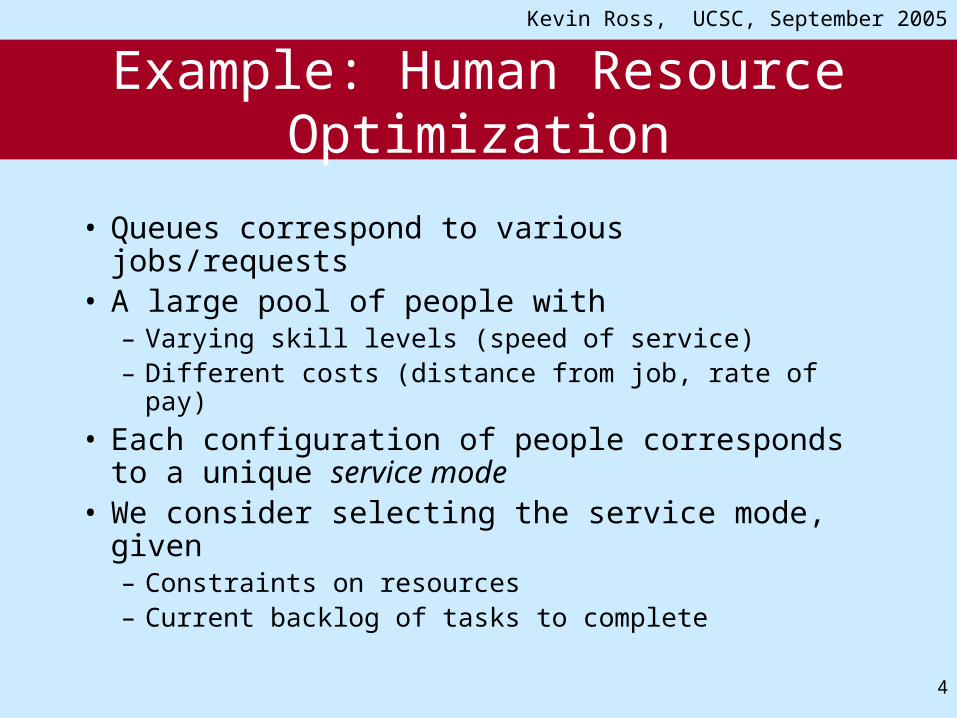
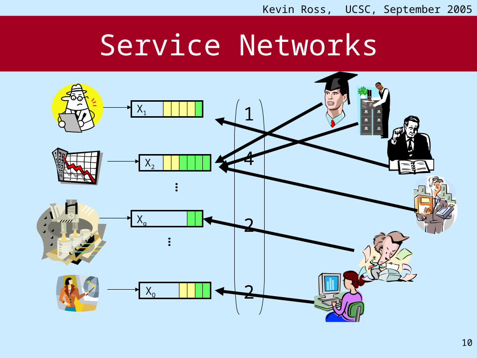
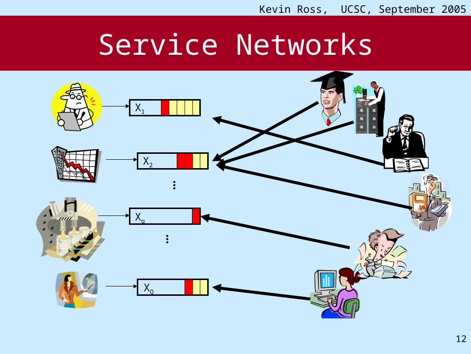
Example: Human Resource Optimization

• Queues correspond to various jobs/requests• A large pool of people with

– Varying skill levels (speed of service)– Different costs (distance from job, rate of pay)

• Each configuration of people corresponds to a unique service mode

• We consider selecting the service mode, given– Constraints on resources– Current backlog of tasks to complete


5

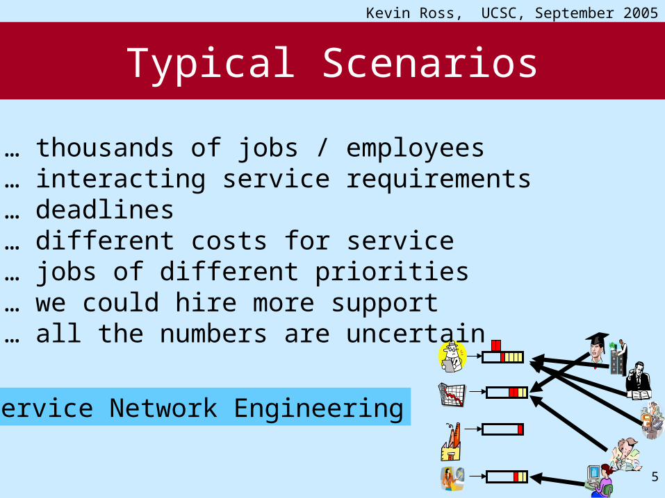
Typical Scenarios

… thousands of jobs / employees … interacting service requirements … deadlines … different costs for service … jobs of different priorities … we could hire more support … all the numbers are uncertain

Service Network Engineering


6

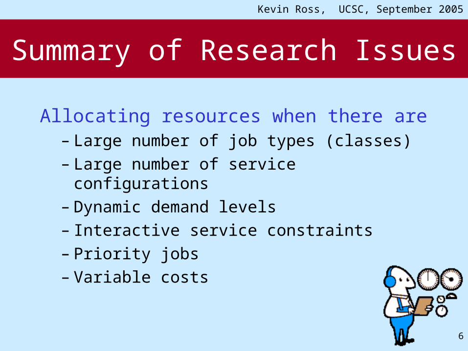
Summary of Research Issues

Allocating resources when there are– Large number of job types (classes)– Large number of service

configurations– Dynamic demand levels– Interactive service constraints– Priority jobs– Variable costs


7

Key Findings

Proved– a large class of scheduling algorithms are

throughput-maximizing for service networks under very general conditions

– we can optimize for quality of service performance

– these algorithms scale well – we can implement the control in a distributed

wayWork in progress

– Tradeoff analysis: • quality of service / load balancing / costs / throughput

– Pricing schemes and value of resources


8

Base Case: Parallel Queue networks

X = workload vector

S = service rate vector

SS = set of all possible service mode vectors

Dynamically select service mode S from S - based on workload X

X1

X2

Xq

XQ

……

Sq

S2

S1

SQ

……

… …


9

Service Networks

X1

X2

Xq

XQ

……


10

Service Networks

X1

X2

Xq

XQ

……

1

4

2

2


11

Service Networks

X1

X2

Xq

XQ

……

1

4

2

2


12

Service Networks

X1

X2

Xq

XQ

……


13

Service Networks

X1

X2

Xq

XQ

……

4

2

1

1


14

What about networks?

1

2

5

3

4

2

Serving one queue creates work in anotherKnown as feedback and forwarding


15

Network of Queues

1

2

3

4

5

2

Feedback and forwarding can be modeled with a similar framework


16

Network of Queues

1

2

3

4

5

2

0 0 1 0 0 0

0 0 0 1 0 0

0 0 0 0 2 0

0 0 0 0 0 1

0 0 0 1 0 0Transfer matrix T

1

2

3

4

5

1 2 3 4 5


17

Network of Queues

1

2

3

4

5

2

0 0 1 0 0 0

0 0 0 1 0 0

0 0 0 0 2 0

0 0 0 0 0 1

0 0 0 1 0 0

0 0 1 2 2

1

1

2

1

1

Arrivals =

Dep

artu

res


18

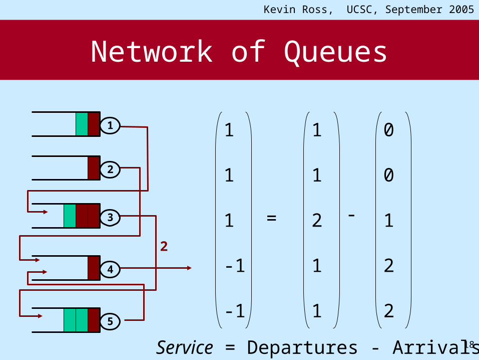
Network of Queues

1

2

3

4

5

2

1

1

1

-1

-1

Service = Departures - Arrivals

0

0

1

2

2

1

1

2

1

1

= -


19

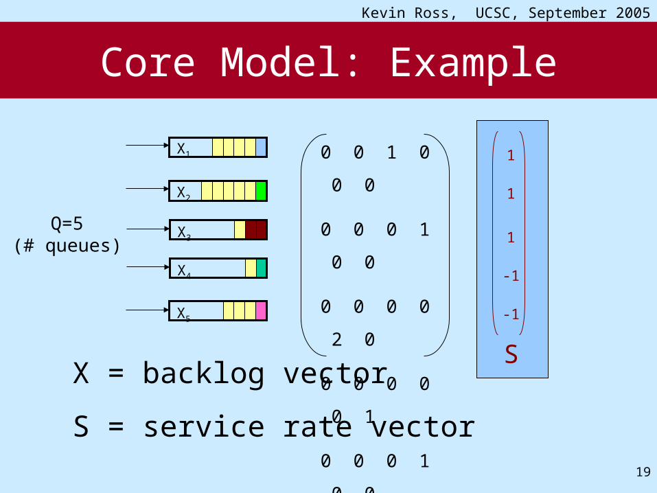
Core Model: Example

X = backlog vector


X1

X2

X3

X5

X4

1

1

1

-1

-1

S

Q=5(# queues)

0 0 1 0 0 0

0 0 0 1 0 0

0 0 0 0 2 0

0 0 0 0 0 1

0 0 0 1 0 0


20

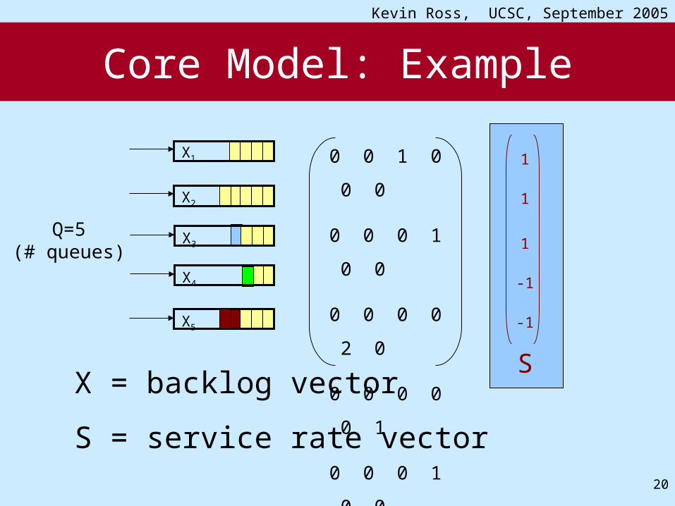
Core Model: Example

X = backlog vector


X1

X2

X3

X5

X4

1

1

1

-1

-1

S

Q=5(# queues)

0 0 1 0 0 0

0 0 0 1 0 0

0 0 0 0 2 0

0 0 0 0 0 1

0 0 0 1 0 0


21

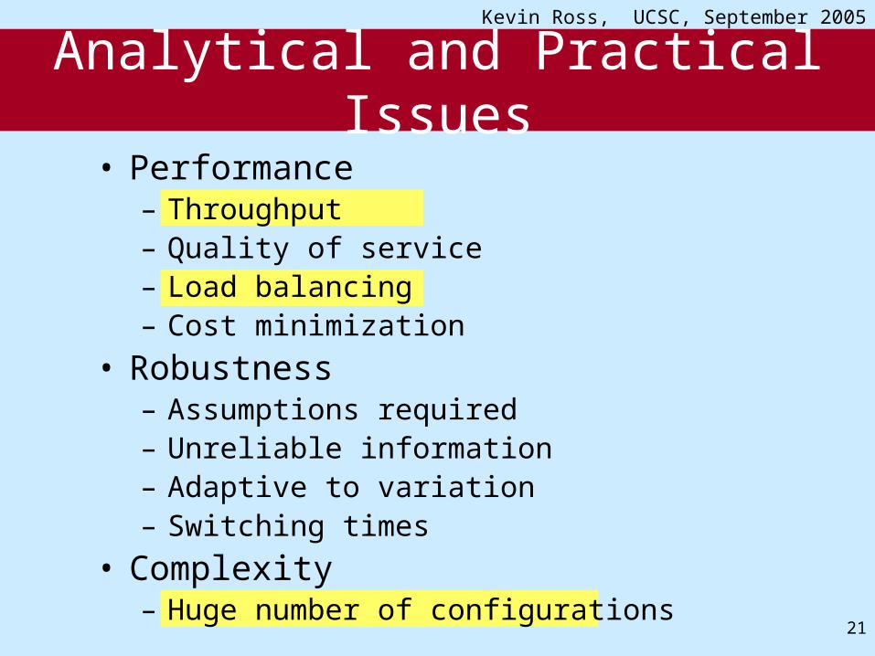
Analytical and Practical Issues• Performance

– Throughput– Quality of service– Load balancing– Cost minimization

• Robustness– Assumptions required– Unreliable information– Adaptive to variation– Switching times

• Complexity– Huge number of configurations


22

System Dynamics

t

tA

tStAtXtX

t

st

1

)(lim

)()()1()(

rate) (Arrival Load

Service)(

Arrival)(

Workload)(

tS

tA

tX

T

tST

tT

1

)(limAIM: Rate Stability:

Notation: Q-vectors

X1

X2

X(t-1)

A(t)

- S(t)

X(t)


23

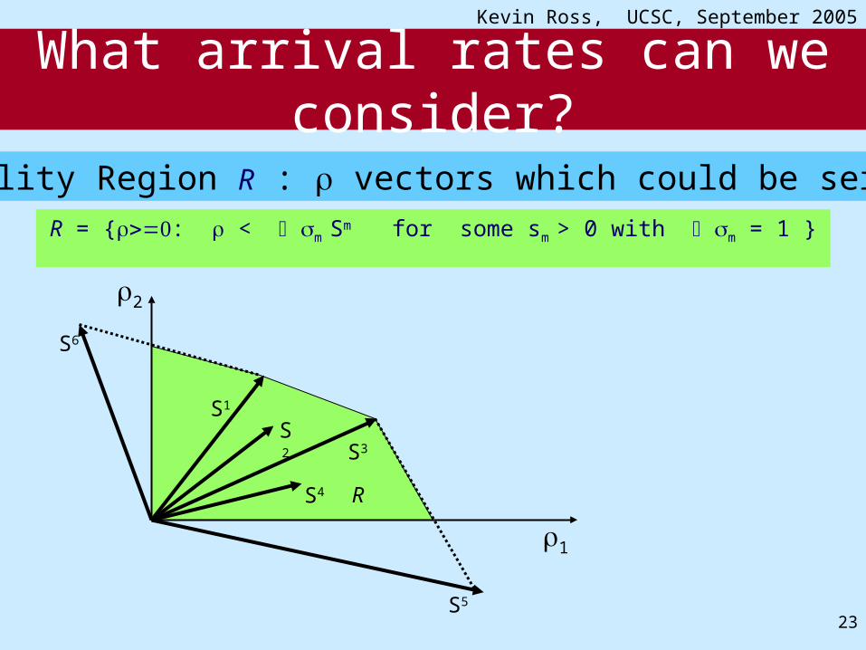
R

What arrival rates can we consider?

1

2

S1

Stability Region R : vectors which could be served

S2

S3

S4

R = {: < m Sm for some sm > 0 with m = 1 }

S6

S5


24

Some Types of Algorithms

Offline• Know the arrival rates in advance• Randomized / Round RobinOnline• Arrival rate is not known• Adapt to Arrivals and Buffer backlog• Two main classes:

– Batch Schedules– Projective Cone Schedules


25

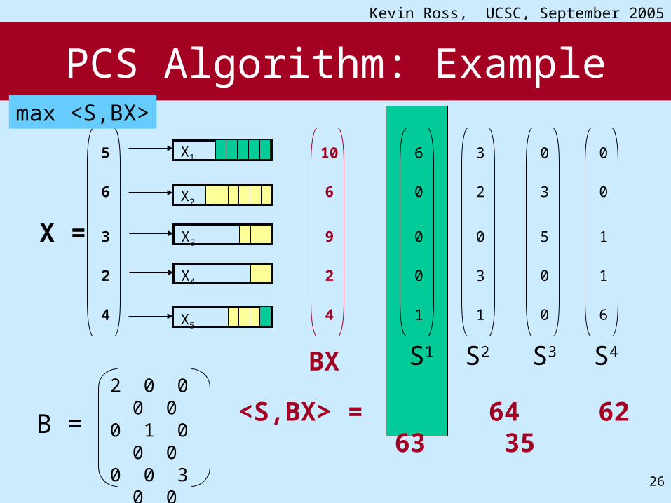
Projective Cone Scheduling (PCS) Algorithms

PCS: When the workload vector is X, choose the service configuration S that maximizes

max < S, BX > over S in SS

For a fixed matrix B that is positive diagonal


26

PCS Algorithm: Example

X1

X2

X3

X5

X4

6

0

0

0

1

3

2

0

3

1

0

3

5

0

0

0

0

1

1

6

S1 S2 S3 S4

5

6

3

2

4

X =

<S,BX> = 64 62 63 35

10

6

9

2

4

BX2 0 0 0 00 1 0 0 00 0 3 0 00 0 0 1 00 0 0 0 1

B =

max <S,BX>


27

When X is in cone C,

choose S = S(C) corresponding to that cone

The set of workload vectors X for which S* maximizes

< S, BX > is a convex cone

X1

X2

S4

S3

S2S1

X

PCS as a Cone Algorithm


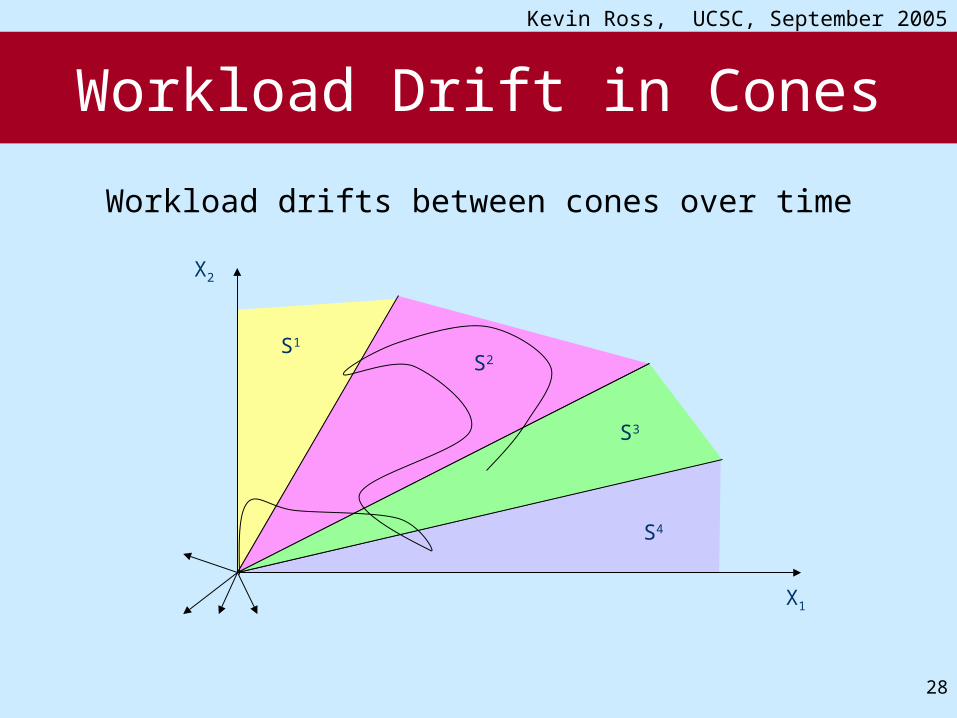
28

Workload Drift in Cones

Workload drifts between cones over time

X1

X2

S4

S3

S2S1


29

What are the Cones?

1

0

0

1

2

1

S

S

1

0

0

2

2

1

S

S

75.0

75.0

1

0

0

1

3

2

1

S

S

S

75.0

75.0

1

0

0

25.1

3

2

1

S

S

S

10

01B

S1

S2

S1

S2

S3


30

Cone Boundaries: Varying B

75.0

75.0

1

0

0

1

3

2

1

S

S

S

10

01B

10

02B

21

12B

S1

S2

S3


31

00.2

0.40.6

0.81

00.2

0.40.6

0.81

0

0.2

0.4

0.6

0.8

1

X1

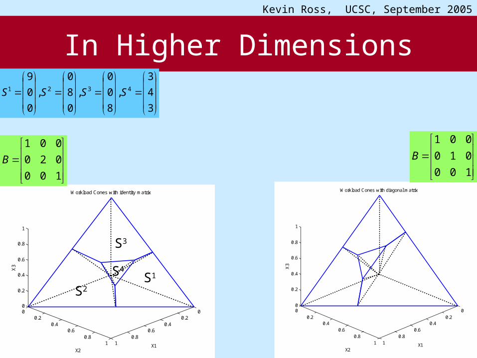
Workload Cones with identity matrix

X2

X3

In Higher Dimensions

100

020

001

B

00.2

0.40.6

0.81

00.2

0.40.6

0.81

0

0.2

0.4

0.6

0.8

1

X1

Workload Cones with diagonal matrix

X2

X3

100

010

001

B

3

4

3

,

8

0

0

,

0

8

0

,

0

0

94321 SSSS

S3

S2S1S4


32

Performance Comparison on Simple Network

0 100 200 300 400 500 600 700 800 900 10000

5

10

15

20

25

30

35

40

45

50Total Workload Comparison

Timeslot

Wor

kloa

d

PCS Algorithm

Randomized AlgorithmRound Robin Algorithm


33

5

5

5

10

0

0

0

10

0

0

0

10

4

3

2

1

S

S

S

S

100

010

001

B

100

010

002

B

175.00

75.010

005.0

B

Performance: Varying Parameters in B


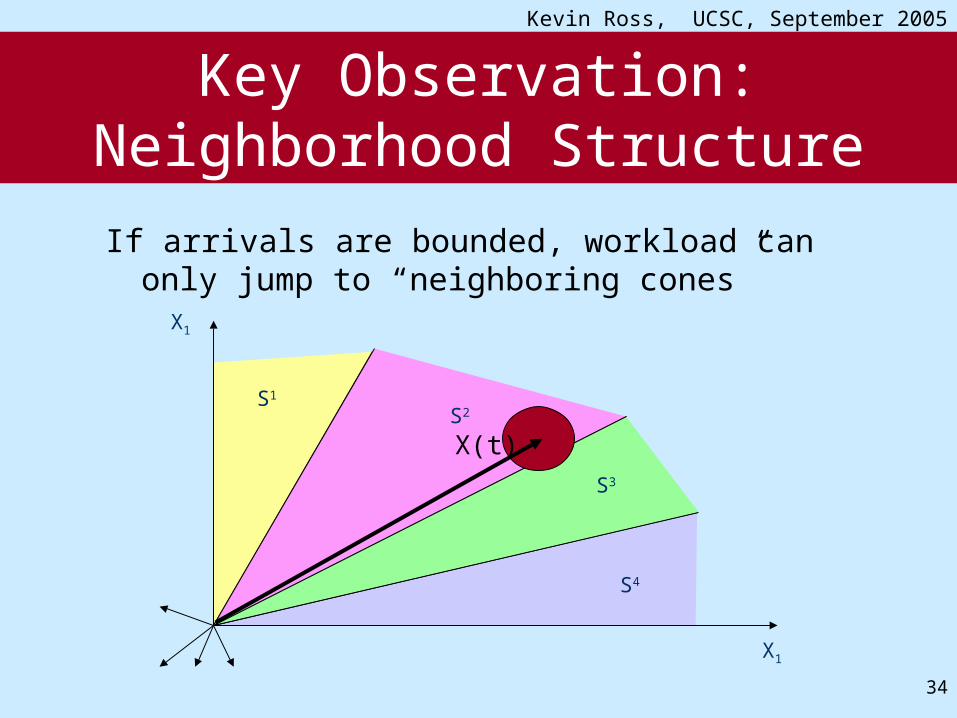
34

Key Observation: Neighborhood Structure

If arrivals are bounded, workload can only jump to “neighboring cones”

X1

X1

S4

S3

S2S1

X(t)


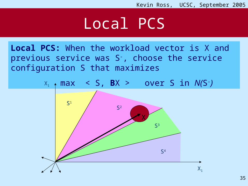
35

Local PCS: When the workload vector is X and previous service was S-, choose the service configuration S that maximizes

max < S, BX > over S in N(S-)

X1

X1

S4

S3

S2S1

Local PCS

X


36

S6

S2

S3

S4

S5

S7

S1

S8

S6

S5

S4

S3

S8

S2

S7

S1

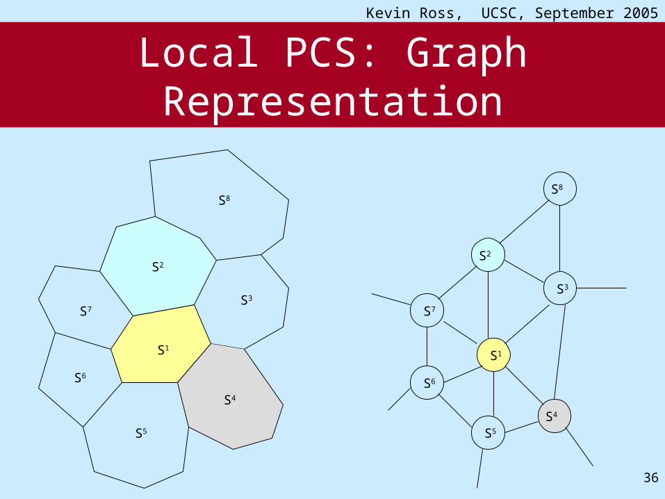
Local PCS: Graph Representation


37

Local PCSS = Permutation Vectors

For crossbar switch


38

Pricing and Resource Valuation

Pricing scenarios:1. We could add a new mode to the set of modes

for a price

2. Each service mode has a different price associated with it

3. It costs to shift modes

When should we pay and how much?


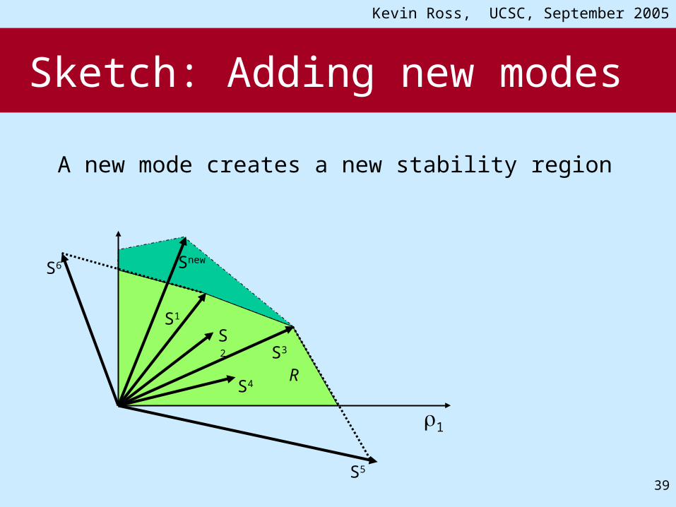
39

Sketch: Adding new modes

A new mode creates a new stability region

R

1

S1

S2

S3

S4

S6

S5

Snew


40

Sketch: Differential pricing

We have price-based stability frontiers

R

1

S1

S2

S3

S4

S6

S5

R2


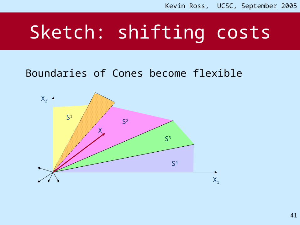
41

Sketch: shifting costs

Boundaries of Cones become flexible

X1

X2

S4

S3

S2S1

X


42

Summary: Service Network Engineering

Resource Management in – Dynamically changing complex networks– Call centers, Utility Computing, Networks,

Workforce, etc.

Challenges– Analytical Concepts of throughput, QoS,

scalability, distributed control– Resource Valuation and Pricing

Kevin Ross, UCSC, September 2005 1 Service Network Engineering Resource Allocation and Optimization...

Documents

Transcript of Kevin Ross, UCSC, September 2005 1 Service Network Engineering Resource Allocation and Optimization...