Ken Black QA 5th chapter 11 Solution
30
Chapter 11: Analysis of Variance and Design of Experiments 1 Chapter 11 Analysis of Variance and Design of Experiments LEARNING OBJECTIVES The focus of this chapter is learning about the design of experiments and the analysis of variance thereby enabling you to: 1. Und erstand the di fferences between vari ous exp er iment des igns a nd when to use them. 2. Comp ut e a nd inte rpre t t he result s of a one -way ANOVA. 3. Comp ut e and inte rpre t t he result s of a random bl oc k des ign. 4. Comp ut e a nd inte rpre t t he result s of a two-way ANOVA. 5. Un derstan d and interpret interaction. 6. Know when and how to us e multi pl e comparison t ec hniq ues. CHAPTER TEACHING STRATEGY This important chapter opens the door for students to a broader view of statistics than they have seen to t his time. Through the topic of experimental designs, the student begins to understand how they can scientifically set up controlled experiments in which to test certain hypotheses. They learn about independent and dependent variables. With the completely randomized design, the student can see how the t test for two independent samples can be expanded to include three or more samples by using analysis of variance. This is something that some of the more curious students were probably wondering about in chapt er 10. Thr ough the randomi zed block desi gn and the fact ori al designs, the student can understand how we can analyze not only multiple categories of one variable, but we can simultaneously analyze multiple variables with several categories each. Thus, this chapter affords the instruct or an opport unity to help the stude nt develop a struc ture for statistical analysis.
-
Upload
rushabh-vora -
Category
Documents
-
view
257 -
download
3
Transcript of Ken Black QA 5th chapter 11 Solution

8/3/2019 Ken Black QA 5th chapter 11 Solution
http://slidepdf.com/reader/full/ken-black-qa-5th-chapter-11-solution 1/30
Chapter 11: Analysis of Variance and Design of Experiments 1
Chapter 11Analysis of Variance and
Design of Experiments
LEARNING OBJECTIVES
The focus of this chapter is learning about the design of experiments and the analysis of
variance thereby enabling you to:
1. Understand the differences between various experiment designs and when to usethem.
2. Compute and interpret the results of a one-way ANOVA.
3. Compute and interpret the results of a random block design.4. Compute and interpret the results of a two-way ANOVA.
5. Understand and interpret interaction.
6. Know when and how to use multiple comparison techniques.
CHAPTER TEACHING STRATEGY
This important chapter opens the door for students to a broader view of statistics
than they have seen to this time. Through the topic of experimental designs, the student begins to understand how they can scientifically set up controlled experiments in which
to test certain hypotheses. They learn about independent and dependent variables. With
the completely randomized design, the student can see how the t test for two independent
samples can be expanded to include three or more samples by using analysis of variance.This is something that some of the more curious students were probably wondering about
in chapter 10. Through the randomized block design and the factorial designs, the
student can understand how we can analyze not only multiple categories of one variable, but we can simultaneously analyze multiple variables with several categories each. Thus,
this chapter affords the instructor an opportunity to help the student develop a structure
for statistical analysis.

8/3/2019 Ken Black QA 5th chapter 11 Solution
http://slidepdf.com/reader/full/ken-black-qa-5th-chapter-11-solution 2/30
Chapter 11: Analysis of Variance and Design of Experiments 2
In this chapter, we emphasize that the total sum of squares in a given problem do
not change. In the completely randomized design, the total sums of squares are parceledinto between treatments sum of squares and error sum of squares. By using a blocking
design when there is significant blocking, the blocking effects are removed from the error
effects which reduceseffect, which reduces the size of the mean square error and can potentially create a more powerful test of the treatment. A similar thing happens in the
two-way factorial design when one significant treatment variable siphons off the sum of
squares from the error term that reduces the mean square error and creates the potentialfor a more powerful test of the other treatment variable.
In presenting the random block design in this chapter, the emphasis is on
determining if the F value for the treatment variable is significant or not. There is a de-emphasis on examining the F value of the blocking effects. However, if the blocking
effects are not significant, the random block design may be a less powerful analysis of the
treatment effects. If the blocking effects are not significant, even though the error sum of
squares is reduced, the mean square error might increase because the blocking effectsmay reduce the degrees of freedom error in a proportionaly greater amount. This might
result in a smaller treatment F value than would occur in a completely randomizeddesign. The repeated-measures design is shown in the chapter as a special case of the
random block design.
In factorial designs, if there are multiple values in the cells, it is possible toanalyze interaction effects. Random block designs do not have multiple values in cells
and therefore interaction effects cannot be calculated. It is emphasized in this chapter
that if significant interaction occurs, then the main effects analysis are confounded andshould not be analyzed in the usual manner. There are various philosophies about how to
handle significant interaction but are beyond the scope of this chapter. The main factorial
example problem in the chapter was created to have no significant interaction so that thestudent can learn how to analyze main effects. The demonstration problem has
significant interaction and these interactions are displayed graphically for the student to
see. You might consider taking this same problem and graphing the interactions usingrow effects along the x axis and graphing the column means for the student to see.
There are a number of multiple comparison tests available. In this text, one of the
more well-known tests, Tukey's HSD, is featured in the case of equal sample sizes.When sample sizes are unequal, a variation on Tukey’s HSD, the Tukey-Kramer test, is
used. MINITAB uses the Tukey testTukey test as one of its options under multiple
comparisons and uses the Tukey-Kramer test for unequal sample sizes. Tukey's HSD isone of the more powerful multiple comparison tests but protectsbut protects less against
Type I errors than some of the other tests.
8/3/2019 Ken Black QA 5th chapter 11 Solution
http://slidepdf.com/reader/full/ken-black-qa-5th-chapter-11-solution 3/30
Chapter 11: Analysis of Variance and Design of Experiments 3
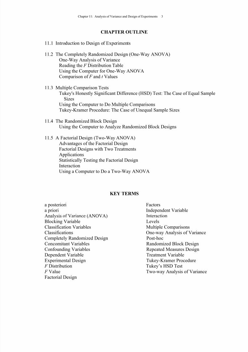
CHAPTER OUTLINE
11.1 Introduction to Design of Experiments
11.2 The Completely Randomized Design (One-Way ANOVA)
One-Way Analysis of VarianceReading the F Distribution Table
Using the Computer for One-Way ANOVA
Comparison of F and t Values
11.3 Multiple Comparison Tests
Tukey's Honestly Significant Difference (HSD) Test: The Case of Equal Sample
SizesUsing the Computer to Do Multiple Comparisons
Tukey-Kramer Procedure: The Case of Unequal Sample Sizes
11.4 The Randomized Block DesignUsing the Computer to Analyze Randomized Block Designs
11.5 A Factorial Design (Two-Way ANOVA)
Advantages of the Factorial Design
Factorial Designs with Two Treatments
ApplicationsStatistically Testing the Factorial Design
Interaction
Using a Computer to Do a Two-Way ANOVA
KEY TERMS
a posteriori Factorsa priori Independent Variable
Analysis of Variance (ANOVA) Interaction
Blocking Variable Levels
Classification Variables Multiple ComparisonsClassifications One-way Analysis of Variance
Completely Randomized Design Post-hoc
Concomitant Variables Randomized Block DesignConfounding Variables Repeated Measures Design
Dependent Variable Treatment Variable
Experimental Design Tukey-Kramer Procedure F Distribution Tukey’s HSD Test
F Value Two-way Analysis of Variance
Factorial Design

8/3/2019 Ken Black QA 5th chapter 11 Solution
http://slidepdf.com/reader/full/ken-black-qa-5th-chapter-11-solution 4/30
Chapter 11: Analysis of Variance and Design of Experiments 4
SOLUTIONS TO PROBLEMS IN CHAPTER 11
11.1 a) Time Period, Market Condition, Day of the Week, Season of the Year
b) Time Period - 4 P.M. to 5 P.M. and 5 P.M. to 6 P.M.
Market Condition - Bull Market and Bear MarketDay of the Week - Monday, Tuesday, Wednesday, Thursday, Friday
Season of the Year – Summer, Winter, Fall, Spring
c) Volume, Value of the Dow Jones Average, Earnings of Investment Houses
11.2 a) Type of 737, Age of the plane, Number of Landings per Week of the plane,City that the plane is based
b) Type of 737 - Type I, Type II, Type III
Age of plane - 0-2 y, 3-5 y, 6-10 y, over 10 y
Number of Flights per Week - 0-5, 6-10, over 10
City - Dallas, Houston, Phoenix, Detroit
c) Average annual maintenance costs, Number of annual hours spent on
maintenance
11.3 a) Type of Card, Age of User, Economic Class of Cardholder, Geographic Region
b) Type of Card - Mastercard, Visa, Discover, American ExpressAge of User - 21-25 y, 26-32 y, 33-40 y, 41-50 y, over 50
Economic Class - Lower, Middle, Upper
Geographic Region - NE, South, MW, West
c) Average number of card usages per person per month,
Average balance due on the card, Average per expenditure per person,
Number of cards possessed per person
11.4 Average dollar expenditure per day/night, Age of adult registering the family,
Number of days stay (consecutive)

8/3/2019 Ken Black QA 5th chapter 11 Solution
http://slidepdf.com/reader/full/ken-black-qa-5th-chapter-11-solution 5/30
Chapter 11: Analysis of Variance and Design of Experiments 5
11.5 Source df SS MS F __
Treatment 2 22.20 11.10 11.07
Error 14 14.03 1.00______
Total 16 36.24
α = .05 Critical F .05,2,14 = 3.74
Since the observed F = 11.07 > F .05,2,14 = 3.74, the decision is to reject the null
hypothesis.
11.6 Source df SS MS F__
Treatment 4 93.77 23.44 15.82Error 18 26.67 1.48______
Total 22 120.43
α = .01 Critical F .01,4,18 = 4.58
Since the observed F = 15.82 > F .01,4,18 = 4.58, the decision is to reject the null
hypothesis.
11.7 Source df SS MS F _
Treatment 3 544.2 181.4 13.00
Error 12 167.5 14.0______
Total 15 711.8
α = .01 Critical F .01,3,12 = 5.95
Since the observed F = 13.00 > F .01,3,12 = 5.95, the decision is to reject the null
hypothesis.
8/3/2019 Ken Black QA 5th chapter 11 Solution
http://slidepdf.com/reader/full/ken-black-qa-5th-chapter-11-solution 6/30
Chapter 11: Analysis of Variance and Design of Experiments 6
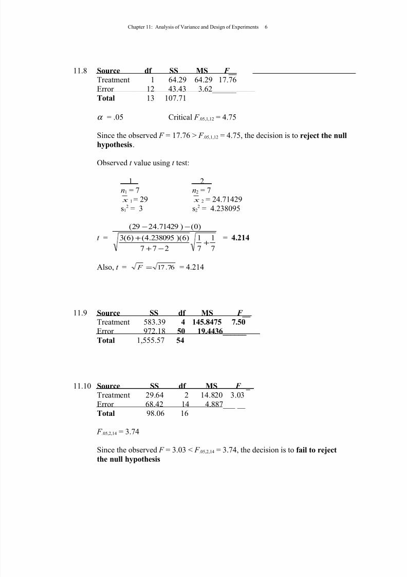
11.8 Source df SS MS F__
Treatment 1 64.29 64.29 17.76
Error 12 43.43 3.62______
Total 13 107.71
α = .05 Critical F .05,1,12 = 4.75
Since the observed F = 17.76 > F .05,1,12 = 4.75, the decision is to reject the null
hypothesis.
Observed t value using t test:
1 2n1 = 7 n2 = 7 x
1 = 29x
2 = 24.71429s12 = 3 s2
2 = 4.238095
t =
7
1
7
1
277
)6)(238095.4()6(3
)0()71429.2429(
+−+
+−−
= 4.214
Also, t = 76.17= F = 4.214
11.9 Source SS df MS F __
Treatment 583.39 4 145.8475 7.50
Error 972.18 50 19.4436______
Total 1,555.57 54
11.10 Source SS df MS F _
Treatment 29.64 2 14.820 3.03
Error 68.42 14 4.887___ __ Total 98.06 16
F .05,2,14 = 3.74
Since the observed F = 3.03 < F .05,2,14 = 3.74, the decision is to fail to reject
the null hypothesis

8/3/2019 Ken Black QA 5th chapter 11 Solution
http://slidepdf.com/reader/full/ken-black-qa-5th-chapter-11-solution 7/30
Chapter 11: Analysis of Variance and Design of Experiments 7
11.11 Source df SS MS F__
Treatment 3 .007076 .002359 10.10
Error 15 .003503 .000234 ________ Total 18 .010579
α = .01 Critical F .01,3,15 = 5.42
Since the observed F = 10.10 > F .01,3,15 = 5.42, the decision is to reject the null
hypothesis.
11.12 Source df SS MS F__ Treatment 2 180700000 90350000 92.67
Error 12 11699999 975000_________
Total 14 192400000
α = .01 Critical F .01,2,12 = 6.93
Since the observed F = 92.67 > F .01,2,12 = 6.93, the decision is to reject the null
hypothesis.
11.13 Source df SS MS F___
Treatment 2 29.61 14.80 11.76
Error 15 18.89 1.26________
Total 17 48.50
α = .05 Critical F .05,2,15 = 3.68
Since the observed F = 11.76 > F .05,2,15 = 3.68, the decison is to reject the null
hypothesis.

8/3/2019 Ken Black QA 5th chapter 11 Solution
http://slidepdf.com/reader/full/ken-black-qa-5th-chapter-11-solution 8/30
Chapter 11: Analysis of Variance and Design of Experiments 8
11.14 Source df SS MS F__
Treatment 3 456630 152210 11.03
Error 16 220770 13798 _______
Total 19 677400
α = .05 Critical F.05,3,16 = 3.24
Since the observed F = 11.03 > F.05,3,16 = 3.24, the decision is to reject the null
hypothesis.
11.15 There are 4 treatment levels. The sample sizes are 18, 15, 21, and 11. The F
value is 2.95 with a p-value of .04. There is an overall significant difference atalpha of .05. The means are 226.73, 238.79, 232.58, and 239.82.
11.16 The independent variable for this study was plant with five classification levels
(the five plants). There were a total of 43 workers who participated in the study.
The dependent variable was number of hours worked per week . An observed F
value of 3.10 was obtained with an associated p-value of .026595. With an alpha
of .05, there was a significant overall difference in the average number of hours
worked per week by plant. A cursory glance at the plant averages revealed thatworkers at plant 3 averaged 61.47 hours per week (highest number) while workersat plant 4 averaged 49.20 (lowest number).
11.17 C = 6 MSE = .3352 α = .05 N = 46
q.05,6,40 = 4.23 n3 = 8 n6 = 7 x 3 = 15.85 x 6 = 17.2
HSD = 4.23
+
71
81
23352. = 0.896
21.1785.1563 −=− x x = 1.36
Since 1.36 > 0.896, there is a significant difference between the means of
groups 3 and 6.

8/3/2019 Ken Black QA 5th chapter 11 Solution
http://slidepdf.com/reader/full/ken-black-qa-5th-chapter-11-solution 9/30
Chapter 11: Analysis of Variance and Design of Experiments 9
11.18 C = 4 n = 6 N = 24 df error = N - C = 24 - 4 = 20 α = .05
MSE = 2.389 q.05,4,20 = 3.96
HSD = qn
MSE = (3.96)6389.2 = 2.50
11.19 C = 3 MSE = 1.002381 α = .05 N = 17 N - C = 14
q.05,3,14 = 3.70 n1 = 6 n2 = 5 x 1 = 2 x 2 = 4.6
HSD = 3.70
+
5
1
6
1
2
002381.1= 1.586
6.4221 −=− x x = 2.6
Since 2.6 > 1.586, there is a significant difference between the means of
groups 1 and 2.
11.20 From problem 11.6, MSE = 1.481481 C = 5 N = 23 N – C = 18
n2 = 5 n4 = 5 α = .01 q.01,5,18 = 5.38
HSD = 5.38
+
5
1
5
1
2
481481.1= 2.93
x 2 = 10 x 4 = 16
161063 −=− x x = 6
Since 6 > 2.93, there is a significant difference in the means of
groups 2 and 4.

8/3/2019 Ken Black QA 5th chapter 11 Solution
http://slidepdf.com/reader/full/ken-black-qa-5th-chapter-11-solution 10/30
Chapter 11: Analysis of Variance and Design of Experiments 10
11.21 N = 16 n = 4 C = 4 N - C = 12 MSE = 13.95833 q.01,4,12 = 5.50
HSD = qn
MSE = 5.50495833.13 = 10.27
x 1 = 115.25 x 2 = 125.25 x 3 = 131.5 x 4 = 122.5
x 1 and x 3 are the only pair that are significantly different using the
HSD test.
11.22 n = 7 C = 2 MSE = 3.619048 N = 14 N - C = 14 - 2 = 12
α = .05 q.05,2,12 = 3.08
HSD = q n
MSE = 3.08
7
619048.3= 2.215
x 1 = 29 and x 2 = 24.71429
Since x 1 - x 2 = 4.28571 > HSD = 2.215, the decision is to reject the null
hypothesis.

8/3/2019 Ken Black QA 5th chapter 11 Solution
http://slidepdf.com/reader/full/ken-black-qa-5th-chapter-11-solution 11/30
Chapter 11: Analysis of Variance and Design of Experiments 11
11.23 C = 4 MSE = .000234 α = .01 N = 19 N – C = 15
q.01,4,15 = 5.25 n1 = 4 n2 = 6 n3 = 5 n4 = 4
x 1 = 4.03, x 2 = 4.001667, x 3 = 3.974, x 4 = 4.005
HSD1,2 = 5.25
+
6
1
4
1
2
000234.= .0367
HSD1,3 = 5.25
+
5
1
4
1
2
000234.= .0381
HSD1,4 = 5.25
+4
1
4
1
2
000234.= .0402
HSD2,3 = 5.25
+
5
1
6
1
2
000234.= .0344
HSD2,4 = 5.25
+
4
1
6
1
2
000234.= .0367
HSD3,4 = 5.25
+
4
1
5
1
2
000234.= .0381
31 x x − = .056
This is the only pair of means that are significantly different .

8/3/2019 Ken Black QA 5th chapter 11 Solution
http://slidepdf.com/reader/full/ken-black-qa-5th-chapter-11-solution 12/30
Chapter 11: Analysis of Variance and Design of Experiments 12
11.24 α = .01 C = 3 n = 5 N = 15 N – C = 12MSE = 975,000 q.01,3,12 = 5.04
HSD = q n
MSE = 5.04
5
000,975= 2,225.6
x 1 = 40,900 x 2 = 49,400 x 3 = 45,300
21 x x − = 8,500
31 x x − = 4,400
32 x x − = 4,100
Using Tukey's HSD, all three pairwise comparisons are significantly different.
11.25 α = .05 C = 3 N = 18 N - C = 15 MSE = 1.259365
q.05,3,15 = 3.67 n1 = 5 n2 = 7 n3 = 6
x 1 = 7.6 x 2 = 8.8571 x 3 = 5.8333
HSD1,2 = 3.67
+
7
1
5
1
2
259365.1= 1.705
HSD1,3 = 3.67
+
6
1
5
1
2
259365.1= 1.763
HSD2,3 = 3.67
+
6
1
7
1
2
259365.1= 1.620
31 x x − = 1.767 (is significant)
32 x x − = 3.024 (is significant)

8/3/2019 Ken Black QA 5th chapter 11 Solution
http://slidepdf.com/reader/full/ken-black-qa-5th-chapter-11-solution 13/30
Chapter 11: Analysis of Variance and Design of Experiments 13
11.26 α = .05 n = 5 C = 4 N = 20 N - C = 16 MSE = 13,798.13
x 1 = 591 x 2 = 350 x 3 = 776 x 4 = 563
HSD = q n
MSE = 4.05
5
13.798,13= 212.76
21 x x − = 241 31 x x − = 185 41 x x − = 28
32 x x − = 426 42 x x − = 213 43 x x − = 213
Using Tukey's HSD = 212.76, means 1 and 2, means 2 and 3, means 2 and 4,
and means 3 and 4 are significantly different.
11.27 α = .05. There were five plants and ten pairwise comparisons. The MINITAB
output reveals that the only significant pairwise difference is between plant 2 and plant 3 where the reported confidence interval (0.180 to 22.460) contains the same
sign throughout indicating that 0 is not in the interval. Since zero is not in the
interval, then we are 95% confident that there is a pairwise differencesignificantly different from zero. The lower and upper values for all other
confidence intervals have different signs indicating that zero is included in the
interval. This indicates that the difference in the means for these pairs might be
zero.
8/3/2019 Ken Black QA 5th chapter 11 Solution
http://slidepdf.com/reader/full/ken-black-qa-5th-chapter-11-solution 14/30
Chapter 11: Analysis of Variance and Design of Experiments 14
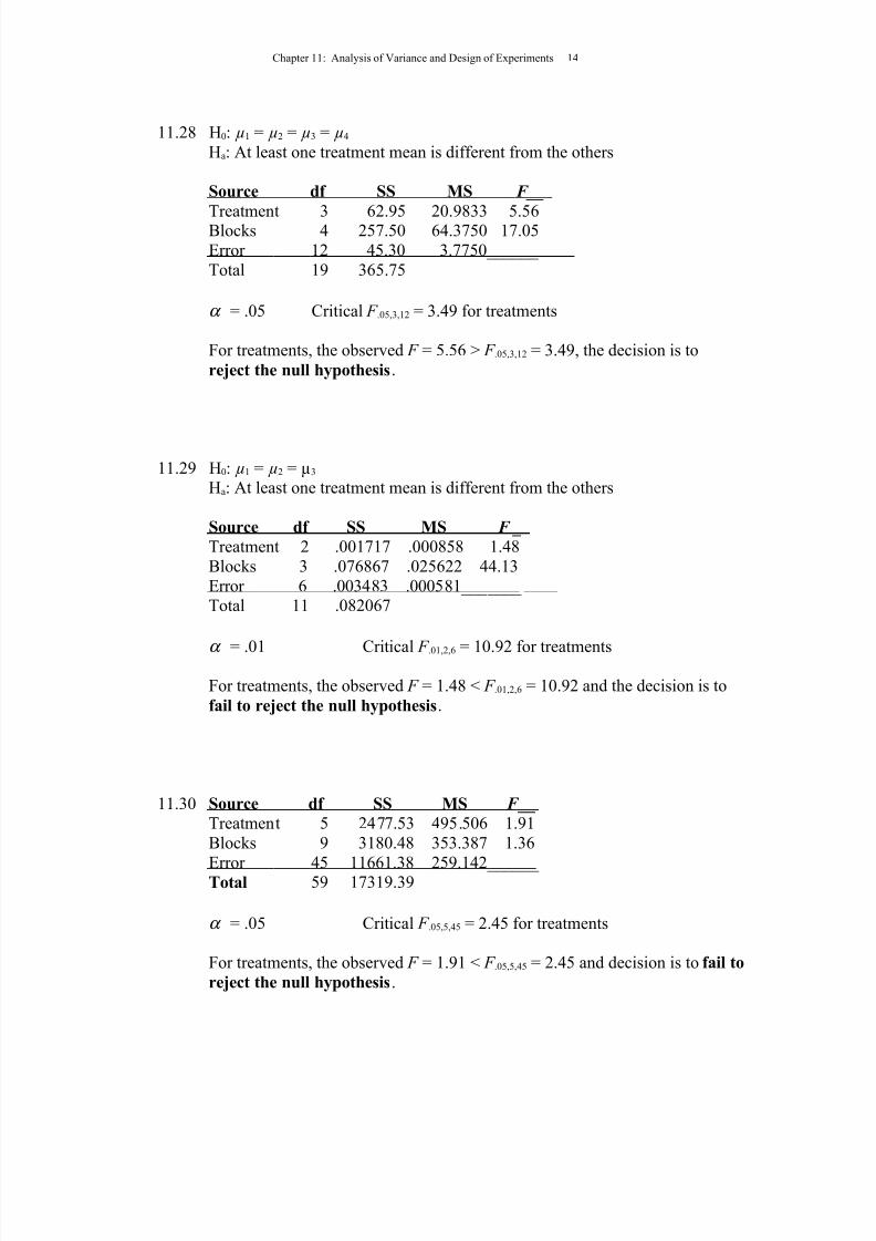
11.28 H0: µ1 = µ2 = µ3 = µ4
Ha: At least one treatment mean is different from the others
Source df SS MS F__
Treatment 3 62.95 20.9833 5.56Blocks 4 257.50 64.3750 17.05
Error 12 45.30 3.7750______
Total 19 365.75
α = .05 Critical F .05,3,12 = 3.49 for treatments
For treatments, the observed F = 5.56 > F .05,3,12 = 3.49, the decision is to
reject the null hypothesis.
11.29 H0: µ1 = µ2 = µ3 Ha: At least one treatment mean is different from the others
Source df SS MS F _
Treatment 2 .001717 .000858 1.48
Blocks 3 .076867 .025622 44.13
Error 6 .003483 .000581_______ Total 11 .082067
α
= .01 Critical F .01,2,6 = 10.92 for treatments
For treatments, the observed F = 1.48 < F .01,2,6 = 10.92 and the decision is to
fail to reject the null hypothesis.
11.30 Source df SS MS F __
Treatment 5 2477.53 495.506 1.91
Blocks 9 3180.48 353.387 1.36
Error 45 11661.38 259.142______ Total 59 17319.39
α = .05 Critical F .05,5,45 = 2.45 for treatments
For treatments, the observed F = 1.91 < F .05,5,45 = 2.45 and decision is to fail to
reject the null hypothesis.
8/3/2019 Ken Black QA 5th chapter 11 Solution
http://slidepdf.com/reader/full/ken-black-qa-5th-chapter-11-solution 15/30
Chapter 11: Analysis of Variance and Design of Experiments 15
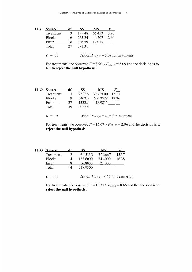
11.31 Source df SS MS F __
Treatment 3 199.48 66.493 3.90Blocks 6 265.24 44.207 2.60
Error 18 306.59 17.033______
Total 27 771.31
α = .01 Critical F .01,3,18 = 5.09 for treatments
For treatments, the observed F = 3.90 < F .01,3,18 = 5.09 and the decision is to
fail to reject the null hypothesis.
11.32 Source df SS MS F__
Treatment 3 2302.5 767.5000 15.67Blocks 9 5402.5 600.2778 12.26
Error 27 1322.5 48.9815____ __ Total 39 9027.5
α = .05 Critical F .05,3,27 = 2.96 for treatments
For treatments, the observed F = 15.67 > F .05,3,27 = 2.96 and the decision is to
reject the null hypothesis.
11.33 Source df SS MS F__
Treatment 2 64.5333 32.2667 15.37
Blocks 4 137.6000 34.4000 16.38Error 8 16.8000 2.1000_ _____
Total 14 218.9300
α = .01 Critical F .01,2,8 = 8.65 for treatments
For treatments, the observed F = 15.37 > F .01,2,8 = 8.65 and the decision is to
reject the null hypothesis.

8/3/2019 Ken Black QA 5th chapter 11 Solution
http://slidepdf.com/reader/full/ken-black-qa-5th-chapter-11-solution 16/30
Chapter 11: Analysis of Variance and Design of Experiments 16
11.34 This is a randomized block design with 3 treatments (machines) and 5 block levels (operators). The F for treatments is 6.72 with a p-value of .019. There is a
significant difference in machines at α = .05. The F for blocking effects is 0.22
with a p-value of .807. There are no significant blocking effects. The blockingeffects reduced the power of the treatment effects since the blocking effects were
not significant.
11.35 The p value for Phone Type, .00018, indicates that there is an overall significant
difference in treatment means at alpha .001. The lengths of calls differ according
to type of telephone used. The p-value for managers, .00028, indicates that there
is an overall difference in block means at alpha .001. The lengths of calls differ
according to Manager. The significant blocking effects have improved the power of the F test for treatments.
11.36 This is a two-way factorial design with two independent variables and one
dependent variable. It is 2x4 in that there are two row treatment levels and four
column treatment levels. Since there are three measurements per cell, interactioncan be analyzed.
df row treatment = 1 df column treatment = 3 df interaction = 3 df error = 16 df total = 23
11.37 This is a two-way factorial design with two independent variables and one
dependent variable. It is 4x3 in that there are four treatment levels and three
column treatment levels. Since there are two measurements per cell, interactioncan be analyzed.
df row treatment = 3 df column treatment = 2 df interaction = 6 df error = 12 df total = 23

8/3/2019 Ken Black QA 5th chapter 11 Solution
http://slidepdf.com/reader/full/ken-black-qa-5th-chapter-11-solution 17/30
Chapter 11: Analysis of Variance and Design of Experiments 17
11.38 Source df SS MS F__
Row 3 126.98 42.327 3.46
Column 4 37.49 9.373 0.77Interaction 12 380.82 31.735 2.60
Error 60 733.65 12.228______
Total 79 1278.94
α = .05
Critical F .05,3,60 = 2.76 for rows. For rows, the observed F = 3.46 > F .05,3,60 = 2.76
and the decision is to reject the null hypothesis.
Critical F .05,4,60 = 2.53 for columns. For columns, the observed F = 0.77 <
F .05,4,60 = 2.53 and the decision is to fail to reject the null hypothesis.
Critical F .05,12,60 = 1.92 for interaction. For interaction, the observed F = 2.60 >
F .05,12,60 = 1.92 and the decision is to reject the null hypothesis.
Since there is significant interaction, the researcher should exercise extremecaution in analyzing the "significant" row effects.
11.39 Source df SS MS F__
Row 1 1.047 1.047 2.40
Column 3 3.844 1.281 2.94
Interaction 3 0.773 0.258 0.59Error 16 6.968 0.436______ Total 23 12.632
α = .05
Critical F .05,1,16 = 4.49 for rows. For rows, the observed F = 2.40 < F .05,1,16 = 4.49
and decision is to fail to reject the null hypothesis.
Critical F .05,3,16 = 3.24 for columns. For columns, the observed F = 2.94 < F .05,3,16 = 3.24 and the decision is to fail to reject the null hypothesis.
Critical F .05,3,16 = 3.24 for interaction. For interaction, the observed F = 0.59 <
F .05,3,16 = 3.24 and the decision is to fail to reject the null hypothesis.
8/3/2019 Ken Black QA 5th chapter 11 Solution
http://slidepdf.com/reader/full/ken-black-qa-5th-chapter-11-solution 18/30
Chapter 11: Analysis of Variance and Design of Experiments 18
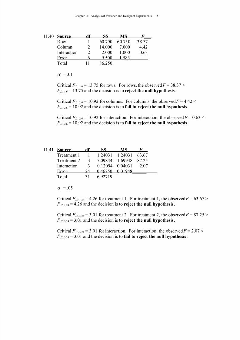
11.40 Source df SS MS F___
Row 1 60.750 60.750 38.37Column 2 14.000 7.000 4.42
Interaction 2 2.000 1.000 0.63
Error 6 9.500 1.583________ Total 11 86.250
α = .01
Critical F .01,1,6 = 13.75 for rows. For rows, the observed F = 38.37 > F .01,1,6 = 13.75 and the decision is to reject the null hypothesis.
Critical F .01,2,6 = 10.92 for columns. For columns, the observed F = 4.42 < F .01,2,6 = 10.92 and the decision is to fail to reject the null hypothesis.
Critical F .01,2,6 = 10.92 for interaction. For interaction, the observed F = 0.63 < F .01,2,6 = 10.92 and the decision is to fail to reject the null hypothesis.
11.41 Source df SS MS F __
Treatment 1 1 1.24031 1.24031 63.67
Treatment 2 3 5.09844 1.69948 87.25Interaction 3 0.12094 0.04031 2.07
Error 24 0.46750 0.01948______
Total 31 6.92719
α = .05
Critical F .05,1,24 = 4.26 for treatment 1. For treatment 1, the observed F = 63.67 > F .05,1,24 = 4.26 and the decision is to reject the null hypothesis.
Critical F .05,3,24 = 3.01 for treatment 2. For treatment 2, the observed F = 87.25 > F .05,3,24 = 3.01 and the decision is to reject the null hypothesis.
Critical F .05,3,24 = 3.01 for interaction. For interaction, the observed F = 2.07 <
F .05,3,24 = 3.01 and the decision is to fail to reject the null hypothesis.
8/3/2019 Ken Black QA 5th chapter 11 Solution
http://slidepdf.com/reader/full/ken-black-qa-5th-chapter-11-solution 19/30
Chapter 11: Analysis of Variance and Design of Experiments 19
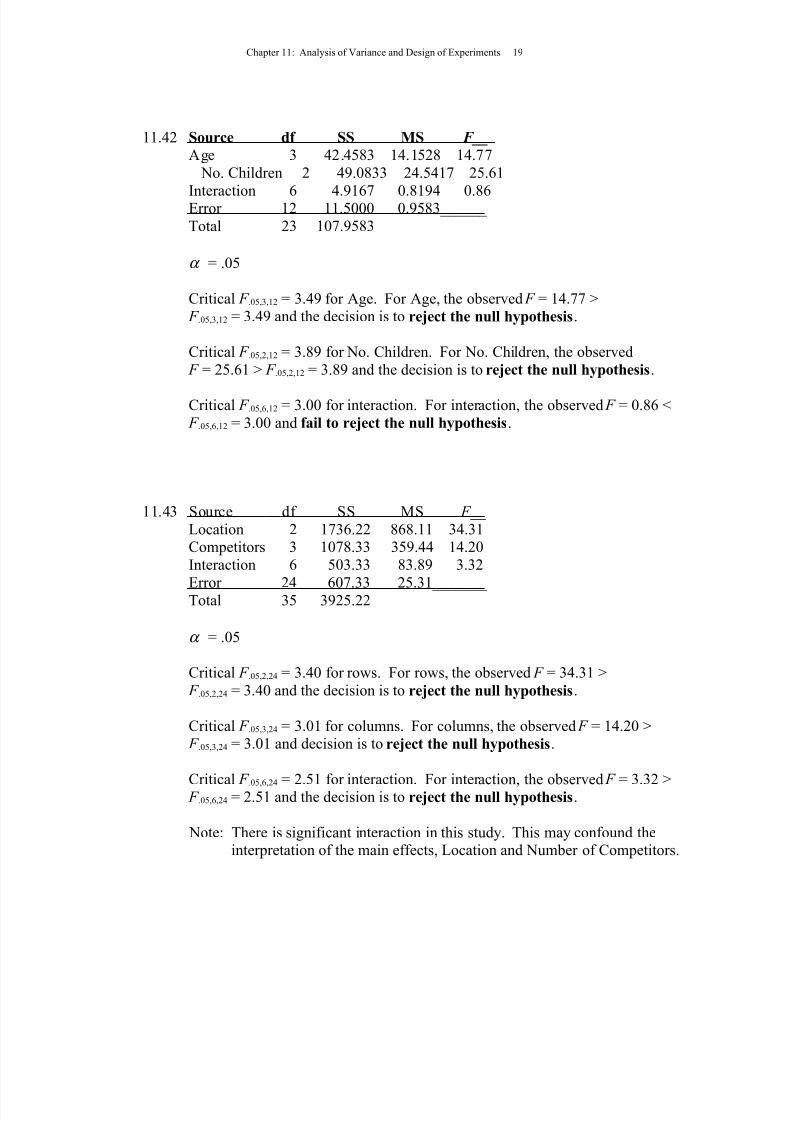
11.42 Source df SS MS F__
Age 3 42.4583 14.1528 14.77
No. Children 2 49.0833 24.5417 25.61
Interaction 6 4.9167 0.8194 0.86Error 12 11.5000 0.9583______
Total 23 107.9583
α = .05
Critical F .05,3,12 = 3.49 for Age. For Age, the observed F = 14.77 > F .05,3,12 = 3.49 and the decision is to reject the null hypothesis.
Critical F .05,2,12 = 3.89 for No. Children. For No. Children, the observed F = 25.61 > F .05,2,12 = 3.89 and the decision is to reject the null hypothesis.
Critical F .05,6,12 = 3.00 for interaction. For interaction, the observed F = 0.86 < F .05,6,12 = 3.00 and fail to reject the null hypothesis.
11.43 Source df SS MS F__
Location 2 1736.22 868.11 34.31Competitors 3 1078.33 359.44 14.20
Interaction 6 503.33 83.89 3.32
Error 24 607.33 25.31_______ Total 35 3925.22
α = .05
Critical F .05,2,24 = 3.40 for rows. For rows, the observed F = 34.31 >
F .05,2,24 = 3.40 and the decision is to reject the null hypothesis.
Critical F .05,3,24 = 3.01 for columns. For columns, the observed F = 14.20 > F .05,3,24 = 3.01 and decision is to reject the null hypothesis.
Critical F .05,6,24 = 2.51 for interaction. For interaction, the observed F = 3.32 > F .05,6,24 = 2.51 and the decision is to reject the null hypothesis.
Note: There is significant interaction in this study. This may confound theinterpretation of the main effects, Location and Number of Competitors.

8/3/2019 Ken Black QA 5th chapter 11 Solution
http://slidepdf.com/reader/full/ken-black-qa-5th-chapter-11-solution 20/30
Chapter 11: Analysis of Variance and Design of Experiments 20
11.44 This two-way design has 3 row treatments and 5 column treatments. There are 45total observations with 3 in each cell.
F R =49.3
16.46=
E
R
MS
MS = 13.23
p-value = .000 and the decision is to reject the null hypothesis for rows.
F C =49.3
70.249=
E
C
MS
MS = 71.57
p-value = .000 and the decision is to reject the null hypothesis for columns.
F I =49.3
27.55=
E
I
MS
MS = 15.84
p-value = .000 and the decision is to reject the null hypothesis for interaction.
Because there is significant interaction, the analysis of main effects is
confounded. The graph of means displays the crossing patterns of the linesegments indicating the presence of interaction.
11.45 The null hypotheses are that there are no interaction effects, that there are nosignificantno significant differences in the means of the valve openings bymachine, and that there are no significant differences in the means of the valve
openings by shift. Since the p-value for interaction effects is .876, there are no
significant interaction effects and that is good since significant interaction effectswould confound that study. The p-value for columns (shifts) is .008 indicating
that column effects are significant at alpha of .01. There is a significant
difference in the mean valve opening according to shift. No multiple comparisons
are given in the output. However, an examination of the shift means indicates thatthe mean valve opening on shift one was the largest at 6.47 followed by shift three
with 6.3 and shift two with 6.25. The p-value for rows (machines) is .937 and that
is not significant.

8/3/2019 Ken Black QA 5th chapter 11 Solution
http://slidepdf.com/reader/full/ken-black-qa-5th-chapter-11-solution 21/30
Chapter 11: Analysis of Variance and Design of Experiments 21
11.46 This two-way factorial design has 3 rows and 3 columns with three observations
per cell. The observed F value for rows is 0.19, for columns is 1.19, and for interaction is 1.40. Using an alpha of .05, the critical F value for rows and
columns (same df) is F 2,18,.05 = 3.55. Neither the observed F value for rows nor the
observed F value for columns is significant. The critical F value for interaction is F 4,18,.05 = 2.93. There is no significant interaction.
11.47 Source df SS MS F__
Treatment 3 66.69 22.23 8.82Error 12 30.25 2.52______
Total 15 96.94
α
= .05 Critical F .05,3,12 = 3.49
Since the treatment F = 8.82 > F .05,3,12 = 3.49, the decision is to reject the null
hypothesis.
For Tukey's HSD:
MSE = 2.52 n = 4 N = 16 C = 4 N - C = 12
q.05,4,12 = 4.20
HSD = qn
MSE = (4.20)452.2 = 3.33
x 1 = 12 x 2 = 7.75 x 3 = 13.25 x 4 = 11.25
Using HSD of 3.33, there are significant pairwise differences between
means 1 and 2, means 2 and 3, and means 2 and 4.
11.48 Source df SS MS F__Treatment 6 68.19 11.365 0.87
Error 19 249.61 13.137______ Total 25 317.80
8/3/2019 Ken Black QA 5th chapter 11 Solution
http://slidepdf.com/reader/full/ken-black-qa-5th-chapter-11-solution 22/30
Chapter 11: Analysis of Variance and Design of Experiments 22
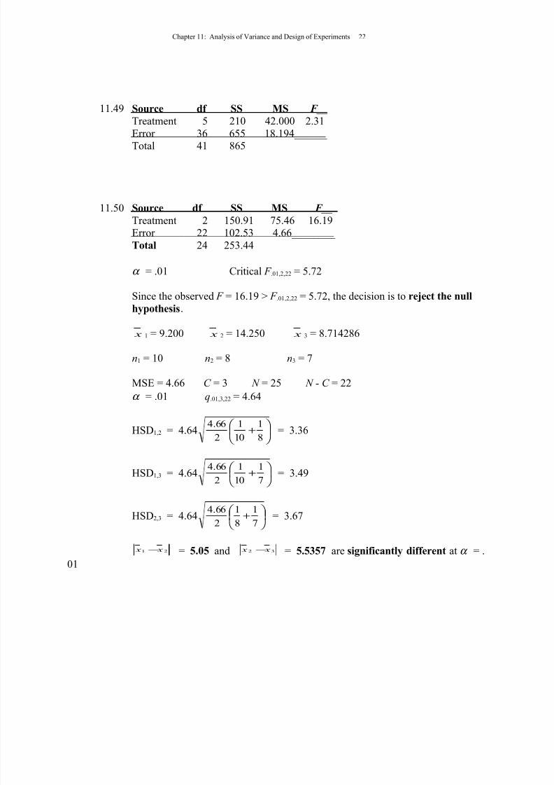
11.49 Source df SS MS F__
Treatment 5 210 42.000 2.31
Error 36 655 18.194______ Total 41 865
11.50 Source df SS MS F__
Treatment 2 150.91 75.46 16.19Error 22 102.53 4.66________
Total 24 253.44
α
= .01 Critical F .01,2,22 = 5.72
Since the observed F = 16.19 > F .01,2,22 = 5.72, the decision is to reject the null
hypothesis.
x 1 = 9.200 x 2 = 14.250 x 3 = 8.714286
n1 = 10 n2 = 8 n3 = 7
MSE = 4.66 C = 3 N = 25 N - C = 22
α = .01 q.01,3,22 = 4.64
HSD1,2 = 4.64
+
8
1
10
1
2
66.4= 3.36
HSD1,3 = 4.64
+
7
1
10
1
2
66.4= 3.49
HSD2,3 = 4.64
+
7
1
8
1
2
66.4= 3.67
21 x x − = 5.05 and 32 x x − = 5.5357 are significantly different at α = .01

8/3/2019 Ken Black QA 5th chapter 11 Solution
http://slidepdf.com/reader/full/ken-black-qa-5th-chapter-11-solution 23/30
Chapter 11: Analysis of Variance and Design of Experiments 23
11.51 This design is a repeated-measures type random block design. There is onetreatment variable with three levels. There is one blocking variable with six
people in it (six levels). The degrees of freedom treatment are two. The degrees
of freedom block are five. The error degrees of freedom are ten. The totaldegrees of freedom are seventeen. There is one dependent variable.
11.52 Source df SS MS F__
Treatment 3 20,994 6998.00 5.58Blocks 9 16,453 1828.11 1.46
Error 27 33,891 1255.22_____
Total 39 71,338
α = .05 Critical F .05,3,27 = 2.96 for treatments
Since the observed F = 5.58 > F .05,3,27 = 2.96 for treatments, the decision is to
reject the null hypothesis.
11.53 Source df SS MS F__
Treatment 3 240.125 80.042 31.51
Blocks 5 548.708 109.742 43.20Error 15 38.125 2.542_ _____ Total 23
α = .05 Critical F .05,3,15 = 3.29 for treatments
Since for treatments the observed F = 31.51 > F .05,3,15 = 3.29, the decision is to
reject the null hypothesis.
For Tukey's HSD:
Ignoring the blocking effects, the sum of squares blocking and sum of squareserror are combined together for a new SSerror = 548.708 + 38.125 = 586.833.
Combining the degrees of freedom error and blocking yields a new df error = 20.
Using these new figures, we compute a new mean square error, MSE =(586.833/20) = 29.34165.
n = 6 C = 4 N = 24 N - C = 20 q.05,4,20 = 3.96

8/3/2019 Ken Black QA 5th chapter 11 Solution
http://slidepdf.com/reader/full/ken-black-qa-5th-chapter-11-solution 24/30
Chapter 11: Analysis of Variance and Design of Experiments 24
HSD = qn
MSE = (3.96)
6
34165.29= 8.757
x 1 = 16.667 x 2 = 12.333 x 3 = 12.333 x 4 = 19.833
None of the pairs of means are significantly different using Tukey's HSD = 8.757.This may be due in part to the fact that we compared means by folding the
blocking effects back into error and the blocking effects were highly
significant.
11.54 Source df SS MS F__
Treatment 1 4 29.13 7.2825 1.98Treatment 2 1 12.67 12.6700 3.44Interaction 4 73.49 18.3725 4.99
Error 30 110.38 3.6793______
Total 39 225.67
α = .05
Critical F .05,4,30 = 2.69 for treatment 1. For treatment 1, the observed F = 1.98 < F .05,4,30 = 2.69 and the decision is to fail to reject the null hypothesis.
Critical F .05,1,30 = 4.17 for treatment 2. For treatment 2 observed F = 3.44 < F .05,1,30 = 4.17 and the decision is to fail to reject the null hypothesis.
Critical F .05,4,30 = 2.69 for interaction. For interaction, the observed F = 4.99 > F .05,4,30 = 2.69 and the decision is to reject the null hypothesis.
Since there are significant interaction effects, examination of the main effects
should not be done in the usual manner. However, in this case, there are nosignificant treatment effects anyway.

8/3/2019 Ken Black QA 5th chapter 11 Solution
http://slidepdf.com/reader/full/ken-black-qa-5th-chapter-11-solution 25/30
Chapter 11: Analysis of Variance and Design of Experiments 25
11.55 Source df SS MS F___
Treatment 2 3 257.889 85.963 38.21
Treatment 1 2 1.056 0.528 0.23Interaction 6 17.611 2.935 1.30
Error 24 54.000 2.250________
Total 35 330.556
α = .01
Critical F .01,3,24 = 4.72 for treatment 2. For the treatment 2 effects, the observed
F = 38.21 > F .01,3,24 = 4.72 and the decision is to reject the null hypothesis.
Critical F .01,2,24 = 5.61 for Treatment 1. For the treatment 1 effects, the observed
F = 0.23 < F .01,2,24 = 5.61 and the decision is to fail to reject the null hypothesis.
Critical F .01,6,24 = 3.67 for interaction. For the interaction effects, the observed F = 1.30 < F .01,6,24 = 3.67 and the decision is to fail to reject the null hypothesis.
11.56 Source df SS MS F___
Age 2 49.3889 24.6944 38.65
Column 3 1.2222 0.4074 0.64
Interaction 6 1.2778 0.2130 0.33Error 24 15.3333 0.6389_______ Total 35 67.2222
α = .05
Critical F .05,2,24 = 3.40 for Age. For the age effects, the observed F = 38.65 > F .05,2,24 = 3.40 and the decision is to reject the null hypothesis.
Critical F .05,3,24 = 3.01 for Region. For the region effects, the observed F = 0.64
< F .05,3,24 = 3.01 and the decision is to fail to reject the null hypothesis.
Critical F .05,6,24 = 2.51 for interaction. For interaction effects, the observed
F = 0.33 < F .05,6,24 = 2.51 and the decision is to fail to reject the null hypothesis.
There are no significant interaction effects. Only the Age effects are significant.
8/3/2019 Ken Black QA 5th chapter 11 Solution
http://slidepdf.com/reader/full/ken-black-qa-5th-chapter-11-solution 26/30
Chapter 11: Analysis of Variance and Design of Experiments 26
Computing Tukey's HSD for Age:
x 1 = 2.667 x 2 = 4.917 x 3 = 2.250
n = 12 C = 3 N = 36 N - C = 33
MSE is recomputed by folding together the interaction and column sum of squares and degrees of freedom with previous error terms:
MSE = (1.2222 + 1.2778 + 15.3333)/(3 + 6 + 24) = 0.5404
q.05,3,33 = 3.49
HSD = q
n
MSE = (3.49)
12
5404.= 0.7406
Using HSD, there are significant pairwise differences between means 1 and 2 and
between means 2 and 3.
Shown below is a graph of the interaction using the cell means by Age.

8/3/2019 Ken Black QA 5th chapter 11 Solution
http://slidepdf.com/reader/full/ken-black-qa-5th-chapter-11-solution 27/30
Chapter 11: Analysis of Variance and Design of Experiments 27
11.57 Source df SS MS F__
Treatment 3 90477679 30159226 7.38Error 20 81761905 4088095_______
Total 23 172000000
α = .05 Critical F .05,3,20 = 3.10
The treatment F = 7.38 > F .05,3,20 = 3.10 and the decision is to reject the null
hypothesis.
11.58 Source df SS MS F__
Treatment 2 460,353 230,176 103.70
Blocks 5 33,524 6,705 3.02Error 10 22,197 2,220_______
Total 17 516,074
α = .01 Critical F .01,2,10 = 7.56 for treatments
Since the treatment observed F = 103.70 > F .01,2,10 = 7.56, the decision is to
reject the null hypothesis.
11.59 Source df SS MS F__
Treatment 2 9.555 4.777 0.46
Error 18 185.1337 10.285_______
Total 20 194.6885
α = .05 Critical F .05,2,18 = 3.55
Since the treatment F = 0.46 > F .05,2,18 = 3.55, the decision is to fail to reject the
null hypothesis.
Since there are no significant treatment effects, it would make no sense tocompute Tukey-Kramer values and do pairwise comparisons.

8/3/2019 Ken Black QA 5th chapter 11 Solution
http://slidepdf.com/reader/full/ken-black-qa-5th-chapter-11-solution 28/30
Chapter 11: Analysis of Variance and Design of Experiments 28
11.60 Source df SS MS F___
Years 2 4.875 2.437 5.16
Size 3 17.083 5.694 12.06
Interaction 6 2.292 0.382 0.81Error 36 17.000 0.472_______
Total 47 41.250
α = .05
Critical F .05,2,36 = 3.32 for Years. For Years, the observed F = 5.16 > F .05,2,36 = 3.32 and the decision is to reject the null hypothesis.
Critical F .05,3,36 = 2.92 for Size. For Size, the observed F = 12.06 > F .05,3,36 = 2.92
and the decision is to reject the null hypothesis.
Critical F .05,6,36 = 2.42 for interaction. For interaction, the observed F = 0.81 < F .05,6,36 = 2.42 and the decision is to fail to reject the null hypothesis.
There are no significant interaction effects. There are significant row and column
effects at α = .05.
11.61 Source df SS MS F___
Treatment 4 53.400 13.350 13.64Blocks 7 17.100 2.443 2.50Error 28 27.400 0.979________
Total 39 97.900
α = .05 Critical F .05,4,28 = 2.71 for treatments
For treatments, the observed F = 13.64 > F .05,4,28 = 2.71 and the decision is to
reject the null hypothesis.
8/3/2019 Ken Black QA 5th chapter 11 Solution
http://slidepdf.com/reader/full/ken-black-qa-5th-chapter-11-solution 29/30
Chapter 11: Analysis of Variance and Design of Experiments 29
11.62 This is a one-way ANOVA with four treatment levels. There are 36 observations
in the study. The p-value of .045 indicates that there is a significant overall
difference in the means at α = .05. An examination of the mean analysis shows
that the sample sizes are different with sizes of 8, 7, 11, and 10, respectively. No
multiple comparison technique was used here to conduct pairwise comparisons.However, a study of sample means shows that the two most extreme means are
from levels one and four. These two means would be the most likely candidates
for multiple comparison tests. Note that the confidence intervals for means oneand four (shown in the graphical output) are seemingly non-overlapping
indicating a potentially significant difference.
11.63 Excel reports that this is a two-factor design without replication indicating that
this is a random block design. Neither the row nor the column p-values are lessthan .05 indicating that there are no significant treatment or blocking effects in
this study. Also displayed in the output to underscore this conclusion are theobserved and critical F values for both treatments and blocking. In both
cases, the observed value is less than the critical value.
11.64 This is a two-way ANOVA with 5 rows and 2 columns. There are 2 observations
per cell. For rows, F R = 0.98 with a p-value of .461 which is not significant. For
columns, F C = 2.67 with a p-value of .134 which is not significant. For interaction, F I = 4.65 with a p-value of .022 which is significant at α = .05.Thus, there are significant interaction effects and the row and column effects are
confounded. An examination of the interaction plot reveals that most of the lines
cross verifying the finding of significant interaction.
11.65 This is a two-way ANOVA with 4 rows and 3 columns. There are 3 observations
per cell. F R = 4.30 with a p-value of .014 is significant at α = .05. The null
hypothesis is rejected for rows. F C = 0.53 with a p-value of .594 is notsignificant. We fail to reject the null hypothesis for columns. F I = 0.99 with a p-value of .453 for interaction is not significant. We fail to reject the null
hypothesis for interaction effects.

8/3/2019 Ken Black QA 5th chapter 11 Solution
http://slidepdf.com/reader/full/ken-black-qa-5th-chapter-11-solution 30/30
Chapter 11: Analysis of Variance and Design of Experiments 30
11.66 This was a random block design with 5 treatment levels and 5 blocking levels. F or both treatment and blocking effects, the critical value is F .05,4,16 = 3.01. The
observed F value for treatment effects is MSC / MSE = 35.98 / 7.36 = 4.89 which
is greater than the critical value. The null hypothesis for treatments is rejected,and we conclude that there is a significant different in treatment means. No
multiple comparisons have been computed in the output. The observed F value
for blocking effects is MSR / MSE = 10.36 /7.36 = 1.41 which is less than thecritical value. There are no significant blocking effects. Using random block
design on this experiment might have cost a loss of power.
11.67 This one-way ANOVA has 4 treatment levels and 24 observations. The F = 3.51yields a p-value of .034 indicating significance at α = .05. Since the sample sizes
are equal, Tukey’s HSD is used to make multiple comparisons. The computer output shows that means 1 and 3 are the only pairs that are significantly different
(same signs in confidence interval). Observe on the graph that the confidence
intervals for means 1 and 3 barely overlap.