Karl W Broman Department of Biostatistics Johns Hopkins University kbroman Gene mapping in model...
51
Karl W Broman Department of Biostatistics Johns Hopkins University http://www.biostat.jhsph.edu/~kbroman Gene mapping in model organisms
-
Upload
marion-osborne -
Category
Documents
-
view
225 -
download
0
Transcript of Karl W Broman Department of Biostatistics Johns Hopkins University kbroman Gene mapping in model...

Karl W Broman
Department of BiostatisticsJohns Hopkins University
http://www.biostat.jhsph.edu/~kbroman
Gene mapping in model organisms

2
Goal
• Identify genes that contribute to common human diseases.

3
Inbred mice

4
Advantages of the mouse
• Small and cheap
• Inbred lines
• Large, controlled crosses
• Experimental interventions
• Knock-outs and knock-ins

5
The mouse as a model
• Same genes?– The genes involved in a phenotype in the mouse may also
be involved in similar phenotypes in the human.
• Similar complexity?– The complexity of the etiology underlying a mouse
phenotype provides some indication of the complexity of similar human phenotypes.
• Transfer of statistical methods.– The statistical methods developed for gene mapping in the
mouse serve as a basis for similar methods applicable in direct human studies.

6
The intercross

7
The data
• Phenotypes, yi
• Genotypes, xij = AA/AB/BB, at genetic markers
• A genetic map, giving the locations of the markers.

8
Phenotypes
133 females
(NOD B6) (NOD B6)

9
NOD

10
C57BL/6
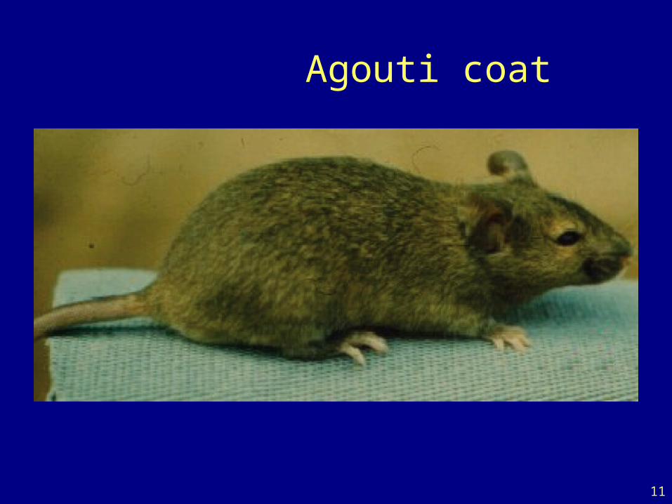
11
Agouti coat

12
Genetic map

13
Genotype data

14
Goals
• Identify genomic regions (QTLs) that contribute to variation in the trait.
• Obtain interval estimates of the QTL locations.
• Estimate the effects of the QTLs.

15
Statistical structure
• Missing data: markers QTL
• Model selection: genotypes phenotype

16
Models: recombination
• No crossover interference– Locations of breakpoints according to a Poisson process.– Genotypes along chromosome follow a Markov chain.
• Clearly wrong, but super convenient.

17
Models: gen phe
Phenotype = y, whole-genome genotype = g
Imagine that p sites are all that matter.
E(y | g) = (g1,…,gp) SD(y | g) = (g1,…,gp)
Simplifying assumptions:
• SD(y | g) = , independent of g
• y | g ~ normal( (g1,…,gp), )
• (g1,…,gp) = + ∑ j 1{gj = AB} + j 1{gj = BB}

18
Before you do anything…
Check data quality
• Genetic markers on the correct chromosomes
• Markers in the correct order
• Identify and resolve likely errors in the genotype data

19
The simplest method
“Marker regression”
• Consider a single marker
• Split mice into groups according to their genotype at a marker
• Do an ANOVA (or t-test)
• Repeat for each marker

20
Marker regression
Advantages
+ Simple
+ Easily incorporates covariates
+ Easily extended to more complex models
Disadvantages
– Must exclude individuals with missing genotypes data
– Imperfect information about QTL location
– Suffers in low density scans
– Only considers one QTL at a time

21
Interval mapping
Lander and Botstein 1989• Imagine that there is a single QTL, at position z.
• Let qi = genotype of mouse i at the QTL, and assume
yi | qi ~ normal( (qi), )
• We won’t know qi, but we can calculate (by an HMM)
pig = Pr(qi = g | marker data)
• yi, given the marker data, follows a mixture of normal distributions with known mixing proportions (the pig).
• Use an EM algorithm to get MLEs of = (AA, AB, BB, ).
• Measure the evidence for a QTL via the LOD score, which is the log10 likelihood ratio comparing the hypothesis of a single QTL at position z to the hypothesis of no QTL anywhere.

22
Interval mapping
Advantages
+ Takes proper account of missing data
+ Allows examination of positions between markers
+ Gives improved estimates of QTL effects
+ Provides pretty graphs
Disadvantages
– Increased computation time
– Requires specialized software
– Difficult to generalize
– Only considers one QTL at a time

23
LOD curves

24
LOD thresholds
• To account for the genome-wide search, compare the observed LOD scores to the distribution of the maximum LOD score, genome-wide, that would be obtained if there were no QTL anywhere.
• The 95th percentile of this distribution is used as a significance threshold.
• Such a threshold may be estimated via permutations (Churchill and Doerge 1994).

25
Permutation test
• Shuffle the phenotypes relative to the genotypes.• Calculate M* = max LOD*, with the shuffled data.• Repeat many times.
• LOD threshold = 95th percentile of M*• P-value = Pr(M* ≥ M)

26
Permutation distribution
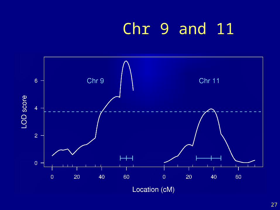
27
Chr 9 and 11

28
Epistasis

29
Going after multiple QTLs
• Greater ability to detect QTLs.
• Separate linked QTLs.
• Learn about interactions between QTLs (epistasis).

30
Multiple QTL mapping
Simplistic but illustrative situation:– No missing genotype data– Dense markers (so ignore positions between markers)– No gene-gene interactions
y = jxj +ε∑ Which j 0?
Model selection in regression

31
Model selection
• Choose a class of models– Additive; pairwise interactions; regression trees
• Fit a model (allow for missing genotype data)– Linear regression; ML via EM; Bayes via MCMC
• Search model space– Forward/backward/stepwise selection; MCMC
• Compare models– BIC() = log L() + (/2) || log n
Miss important loci include extraneous loci.

32
Special features
• Relationship among the covariates
• Missing covariate information
• Identify the key players vs. minimize prediction error

33
Opportunities for improvements
• Each individual is unique.
– Must genotype each mouse.
– Unable to obtain multiple invasive phenotypes (e.g., in multiple environmental conditions) on the same genotype.
• Relatively low mapping precision.
Design a set of inbred mouse strains.
– Genotype once.
– Study multiple phenotypes on the same genotype.

34
Recombinant inbred lines

35
AXB/BXA panel
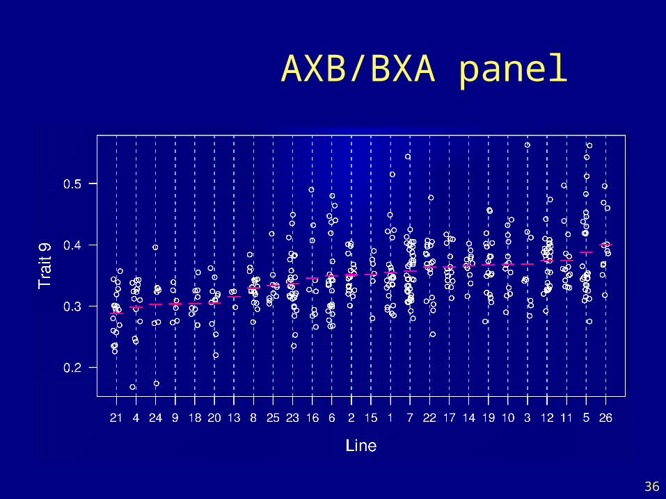
36
AXB/BXA panel

37
LOD curves
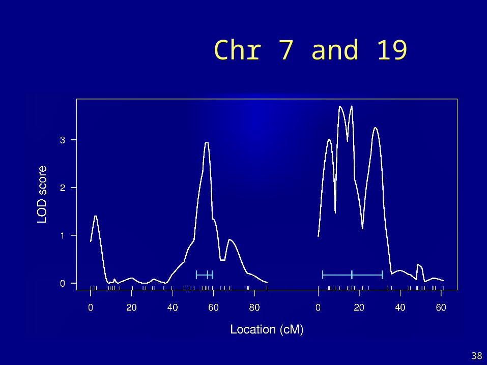
38
Chr 7 and 19
39
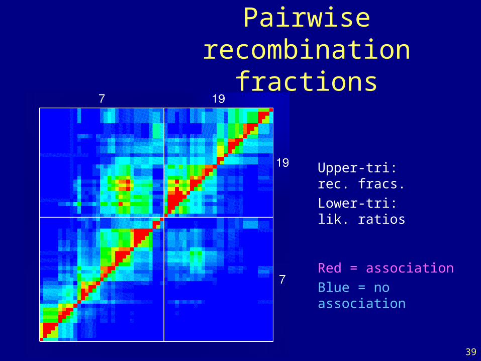
Pairwiserecombination fractions
Upper-tri: rec. fracs.
Lower-tri: lik. ratios
Red = association
Blue = no association

40
RI lines
Advantages
• Each strain is a eternal resource.
– Only need to genotype once.
– Reduce individual variation by phenotyping multiple individuals from each strain.
– Study multiple phenotypes on the same genotype.
• Greater mapping precision.
Disadvantages
• Time and expense.
• Available panels are generally too small (10-30 lines).
• Can learn only about 2 particular alleles.
• All individuals homozygous.

41
The RIX design

42
The “Collaborative Cross”

43
Genome of an 8-way RI

44
The “Collaborative Cross”
Advantages
• Great mapping precision.
• Eternal resource.
– Genotype only once.
– Study multiple invasive phenotypes on the same genotype.
Barriers
• Advantages not widely appreciated.
– Ask one question at a time, or Ask many questions at once?
• Time.
• Expense.
• Requires large-scale collaboration.

45
To be worked out
• Breakpoint process along an 8-way RI chromosome.
• Reconstruction of genotypes given multipoint marker data.
• QTL analyses.
– Mixed models, with random effects for strains and genotypes/alleles.
• Power and precision (relative to an intercross).

46
Haldane & Waddington 1931
r = recombination fraction per meiosis between two loci
AutosomesPr(G1=AA) = Pr(G1=BB) = 1/2
Pr(G2=BB | G1=AA) = Pr(G2=AA | G1=BB) = 4r / (1+6r)
X chromosomePr(G1=AA) = 2/3 Pr(G1=BB) = 1/3
Pr(G2=BB | G1=AA) = 2r / (1+4r)
Pr(G2=AA | G1=BB) = 4r / (1+4r)
Pr(G2 G1) = (8/3) r / (1+4r)

47
8-way RILs
AutosomesPr(G1 = i) = 1/8
Pr(G2 = j | G1 = i) = r / (1+6r) for i j
Pr(G2 G1) = 7r / (1+6r)
X chromosomePr(G1=AA) = Pr(G1=BB) = Pr(G1=EE) = Pr(G1=FF) =1/6
Pr(G1=CC) = 1/3
Pr(G2=AA | G1=CC) = r / (1+4r)
Pr(G2=CC | G1=AA) = 2r / (1+4r)
Pr(G2=BB | G1=AA) = r / (1+4r)
Pr(G2 G1) = (14/3) r / (1+4r)

48
Areas for research
• Model selection procedures for QTL mapping
• Gene expression microarrays + QTL mapping
• Combining multiple crosses
• Association analysis: mapping across mouse strains
• Analysis of multi-way recombinant inbred lines

49
References
• Broman KW (2001) Review of statistical methods for QTL mapping in experimental crosses. Lab Animal 30:44–52
• Jansen RC (2001) Quantitative trait loci in inbred lines. In Balding DJ et al., Handbook of statistical genetics, Wiley, New York, pp 567–597
• Lander ES, Botstein D (1989) Mapping Mendelian factors underlying quantitative traits using RFLP linkage maps. Genetics 121:185 – 199
• Churchill GA, Doerge RW (1994) Empirical threshold values for quantitative trait mapping. Genetics 138:963–971
• Kruglyak L, Lander ES (1995) A nonparametric approach for mapping quantitative trait loci. Genetics 139:1421-1428
• Broman KW (2003) Mapping quantitative trait loci in the case of a spike in the phenotype distribution. Genetics 163:1169–1175
• Miller AJ (2002) Subset selection in regression, 2nd edition. Chapman & Hall, New York

50
More references• Broman KW, Speed TP (2002) A model selection approach for the
identification of quantitative trait loci in experimental crosses (with discussion). J R Statist Soc B 64:641-656, 737-775
• Zeng Z-B, Kao C-H, Basten CJ (1999) Estimating the genetic architecture of quantitative traits. Genet Res 74:279-289
• Mott R, Talbot CJ, Turri MG, Collins AC, Flint J (2000) A method for fine mapping quantitative trait loci in outbred animal stocks. Proc Natl Acad Sci U S A 97:12649-12654
• Mott R, Flint J (2002) Simultaneous detection and fine mapping of quantitative trait loci in mice using heterogeneous stocks. Genetics 160:1609-1618
• The Complex Trait Consortium (2004) The Collaborative Cross, a community resource for the genetic analysis of complex traits. Nature Genetics 36:1133-1137
• Broman KW. The genomes of recombinant inbred lines. Genetics, in press
51
Software
• R/qtlhttp://www.biostat.jhsph.edu/~kbroman/qtl
• Mapmaker/QTLhttp://www.broad.mit.edu/genome_software
• Mapmanager QTXhttp://www.mapmanager.org/mmQTX.html
• QTL Cartographerhttp://statgen.ncsu.edu/qtlcart/index.php
• Multimapperhttp://www.rni.helsinki.fi/~mjs