Karl Pearson and the Chi-Squared TestAuthor(s): R. L. PlackettReviewed work(s):Source: International Statistical Review / Revue Internationale de Statistique, Vol. 51, No. 1(Apr., 1983), pp. 59-72Published by: International Statistical Institute (ISI)Stable URL: http://www.jstor.org/stable/1402731 .Accessed: 27/09/2012 05:02

Your use of the JSTOR archive indicates your acceptance of the Terms & Conditions of Use, available at .http://www.jstor.org/page/info/about/policies/terms.jsp

.JSTOR is a not-for-profit service that helps scholars, researchers, and students discover, use, and build upon a wide range ofcontent in a trusted digital archive. We use information technology and tools to increase productivity and facilitate new formsof scholarship. For more information about JSTOR, please contact support@jstor.org.

.

International Statistical Institute (ISI) is collaborating with JSTOR to digitize, preserve and extend access toInternational Statistical Review / Revue Internationale de Statistique.

http://www.jstor.org

International Statistical Review, 51 (1983), pp. 59-72. Longman Group Limited/Printed in Great Britain

? International Statistical Institute

Karl Pearson and the Chi-squared Test

R.L. Plackett

Department of Statistics, The University, Newcastle upon Tyne NE1 7RU, UK

Summary

Pearson's paper of 1900 introduced what subsequently became known as the chi-squared test of goodness of fit. The terminology and allusions of 80 years ago create a barrier for the modern reader, who finds that the interpretation of Pearson's test procedure and the assessment of what he achieved are less than straightforward, notwithstanding the technical advances made since then. An attempt is made here to surmount these difficulties by exploring Pearson's relevant activities during the first decade of his statistical career, and by describing the work by his contemporaries and predecessors which seem to have influenced his approach to the problem. Not all the questions are answered, and others remain for further study.

Key words: Bravais; Degrees of freedom; Edgeworth; Goodness of fit; Large deviations; Multino- mial distribution; Multivariate error law; Multivariate normal density; Runs at roulette; Small probability density.

1 Introduction

Karl Pearson was a man of many parts: the applied mathematician who completed Todhunter's History of the Theory of Elasticity; the philosopher of science whom Lenin described as 'this conscientious and honest opponent of materialism' (1970, p. 170); the statistician who espoused the cause of evolution and edited Biometrika for 35 years; the innovator and administrator whose Department became famous and influential; the tireless contributor to the British war effort during 1914-18; the employer who gave scientific work to women at a time when this was exceptional; and the family man who returned to seek his ancestry among the dales of the North York Moors.

When Pearson was 33 years of age, his career began to change as a consequence of two events:

(I) the publication in 1889 of Galton's book Natural Inheritance; (II) the appointment in 1890 of Weldon to the Chair of Zoology at University

College London.

Galton was led to his work on regression and correlation by interests in psychology, heredity, and anthropology. Weldon was impressed by Darwin's theory of natural selec- tion, and had used elementary statistical methods, assisted by Galton. He established contact with Pearson, provided data for analysis, and encouraged theoretical develop- ments.

During the period 1891-1900, Pearson's energies were mainly concentrated on further- ing the study and applications of correlation and regression. In 1900 there appeared his paper on the chi-squared test of goodness of fit. Everyone agrees that such procedures now form an essential part of statistical method. But few people read the paper, and those who do find that the terminology and allusions pose questions to be resolved and possibly answered. These questions are considered in what follows, where the objectives are

60 R.L. PLACKETT

threefold: an exploration of Pearson's relevant activities during the first decade of his statistical career; a description of the work by his contemporaries and predecessors which directly or indirectly influenced his approach to the problem; and an attempt to interpret his test procedure and place his achievement in the context of statistical knowledge at the time.

2 Goodness of fit

When Pearson applied for the Gresham Lectureship in Geometry in November 1890, he included graphical statistics and the theory of probability and insurance among the topics on which he proposed to speak. The lectures on 'The Geometry of Statistics' were given in November 1891, January 1892, and May 1892. They contained a full account of graphical methods. The lectures on 'The Laws of Chance' were given in November 1892 and early in 1893. They were based on as much experimental evidence and as little theory as possible. No doubt the time of the lectures (6 pm) and the audience of 'clerks and others engaged during the day in the City' determined his approach. Another influence must have been Edgeworth's Newmarch Lectures, given in June 1892, which covered prob- abilistic assessment of empirical evidence. Pearson had received the syllabus from Edgeworth (they corresponded on statistics at this time) and it is likely that he attended.

The following details on his methods of collecting and interpreting experimental evidence are obtained by collating the syllabuses reproduced by E.S. Pearson (1938) with Chapter 2 of K. Pearson (1897a). This chapter is entitled 'The scientific aspect of Monte Carlo roulette' and is essentially the same as an article on 'Science and Monte Carlo' which appeared in February 1894.

Pearson occupied part of the vacation of 1892 with 2400 tosses of ten shillings at a time 'frequently in the open air'. His former pupil, Mr C.L.T. Griffith supplemented the shilling results with 8178 tosses of a penny, and 1000 drawings of nine tickets from a bag containing 90 tickets, ten of each digit. Further material was required, and a friend suggested the Monte Carlo roulette tables. But how could the material be obtained? The

Royal Society or British Association were unlikely to award a grant for the expenses of a

stay of several months in Monte Carlo. Luckily, records were published in Le Monaco, available weekly in Paris at a cost of one franc.

Pearson's analysis of these artificial experiments depends on considering 'deviations from the most probable' in relation to the 'standard deviation', a term which first appears in his lecture syllabus for 31 January 1893. If the laws of chance apply to Monte Carlo roulette, then several consequences follow:

(a) Black and red are equally likely when the zero is excluded. (b) All 37 numbers are equiprobable. (c) Runs of the same colour follow a geometric distribution.

Pearson accepted the first hypothesis. As regards the second, he took 16563 throws from four weeks' play and compared the standard deviation of the observed frequencies (15.85) with the theoretical standard deviation (20.87) by finding 'the standard deviation of the standard deviation'

(o-,2n = 2.43). He interpreted the results to mean a divergence

between experiment and theory. The individual frequencies have not survived, but his value of the theoretical standard deviation is easily confirmed, being that for a binomial distribution.

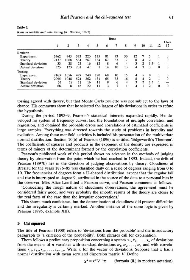
Table 1 relates to the third hypothesis and shows the distribution of runs for 4274 trials at roulette and 4191 tosses of a penny. Pearson inspected each class and derived probabilities from a normal approximation to the binomial distribution. He found that

Karl Pearson and the chi-squared test 61

Table 1 Runs in roulette and coin tossing (K. Pearson, 1897)

Runs Over

1 2 3 4 5 6 7 8 9 10 11 12 12

Roulette Experiment 2462 945 333 220 135 81 43 30 12 7 5 1 0 Theory 2137 1068 534 267 134 67 33 17 8 4 2 1 0 Standard deviation 33 28 22 16 12 8 6 4 3 2 1.5 1 -

Actual deviation 325 123 201 47 1 14 10 13 4 3 3 0 0 Tossing

Experiment 2163 1056 479 240 120 68 40 15 4 5 0 1 0 Theory 2095 1048 524 262 131 65 33 16 8 4 2 1 0 Standard deviation 32 28 21 16 11 8 6 4 3 2 1.5 1 Actual deviation 68 8 45 22 11 3 7 1 4 1 2 0 0

tossing agreed with theory, but that Monte Carlo roulette was not subject to the laws of chance. His comments show that he selected the largest of his deviations in order to refute the hypothesis.

During the period 1893-9, Pearson's statistical interests expanded rapidly. He de- veloped his system of frequency curves, laid the foundations of multiple correlation and regression, and obtained the probable errors and correlations of estimated coefficients in large samples. Everything was directed towards the study of problems in heredity and evolution. Among these manifold activities is included his presentation of the multivariate normal distribution. Section 10(b) of Pearson (1896) is entitled 'Edgeworth's Theorem'. The coefficients of squares and products in the exponent of the density are expressed in terms of minors of the determinant formed by the correlation coefficients.

Pearson's published work of this period shows no advance in the methods of judging theory by observation from the point which he had reached in 1893. Indeed, the drift of Pearson (1897b) lies in the direction of judging observations by theory. Cloudiness at Breslau for the years 1876-85 was classified daily on a scale of degrees ranging from 0 to 10. The frequencies of degrees form a U-shaped distribution, except that the regular fall and rise is interrupted at degree 9, attributed in the source of the data to a personal bias in the observer. Miss Alice Lee fitted a Pearson curve, and Pearson comments as follows.

'Considering the rough nature of cloudiness observations, the agreement must be considered fairly good, and very probably the smooth results of the theory are closer to the real facts of the case than the irregular observations.'

This shows much confidence, but the determination of cloudiness did present difficulties and the irregularity is certainly marked. Another instance of the same logic is given by Pearson (1895, example XII).

3 Chi squared The title of Pearson (1900) refers to 'deviations from the probable' and the introductory paragraph to 'a criterion of the probability'. Both phrases call for explanation.

There follows a preliminary proposition concerning a system x1, x2,... , x, of deviations from the means of n variables with standard deviations at2, 2 *,..., *a, and with correla- tions r12, r13, r23,..., rn-1,,. Write x for the vector of deviations. Suppose that x has a normal distribution with mean zero and dispersion matrix V. Define

2 = xTV-1x (formula (ii.) in modern notation).

62 R.L. PLACKETr

'Then: X2 = constant, is the equation to a generalised 'ellipsoid', all over the surface of which the frequency of the system of errors or deviations x1, x2,... , x,* is constant. The values which X must be given to cover the whole of space are from 0 to oo.'

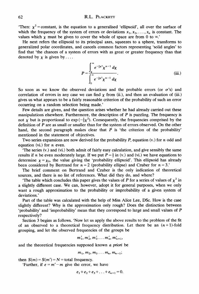
He next refers the ellipsoid to its principal axes, squeezes to a sphere, transforms to generalized polar coordinates, and cancels common factors representing 'solid angles' to find that 'the chances of a system of errors with as great or greater frequency than that denoted by X is given by....

Je-•2Xn-1

dX P = (iii.)

je-?X2x-1 dX

So soon as we know the observed deviations and the probable errors (or tr's) and correlation of errors in any case we can find X from (ii.), and then an evaluation of (iii.) gives us what appears to be a fairly reasonable criterion of the probability of such an error occurring on a random selection being made.'

Few details are given, and the question arises whether he had already carried out these manipulations elsewhere. Furthermore, the description of P is puzzling. The frequency is not X but is proportional to exp (-IX2). Consequently, the frequencies comprised by the definition of P are as small or smaller than for the system of errors observed. On the other hand, the second paragraph makes clear that P is 'the criterion of the probability' mentioned in the statement of objectives.

Two series expansions are now derived for the probability P, equation (v.) for n odd and equation (vi.) for n even.

'The series (v.) and (vi.) both admit of fairly easy calculation, and give sensibly the same results if n be even moderately large. If we put P = - in (v.) and (vi.) we have equations to determine X = Xo, the value giving the 'probability ellipsoid'. This ellipsoid has already been considered by Bertrand for n = 2 (probability ellipse) and Czuber for n = 3.'

The brief comment on Bertrand and Czuber is the only indication of theoretical sources, and there is no list of references. What did they do, and where?

'The table which concludes this paper gives the values of P for a series of values of X2 in a slightly different case. We can, however, adopt it for general purposes, when we only want a rough approximation to the probability or improbability of a given system of deviations.'

Part of the table was calculated with the help of Miss Alice Lee, DSc. How is the case slightly different? Why is the approximation only rough? Does the distinction between 'probability' and 'improbability' mean that they correspond to large and small values of P respectively?

Section 3 begins as follows. 'Now let us apply the above results to the problem of the fit of an observed to a theoretical frequency distribution. Let there be an (n + 1)-fold grouping, and let the observed frequencies of the groups be

'n1, 'n2, m'3 ... m/, mn,

and the theoretical frequencies supposed known a priori be

m1, m2, 13

. .* ,

* ,n+l;

then S(m) = S(m') = N = total frequency. 'Further, if e = m'- m give the error, we have

el + e2+ e3+ ... + e,+l =0.

Karl Pearson and the chi-squared test 63

Hence only n of the n + 1 errors are variables; the (n + 1)-th is determined when the first n are known, and in using formula (ii.) we treat only of n variables.'

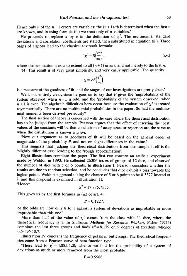
He proceeds to replace x by e in the definition of X2. The multinomial standard deviations and correlation coefficients are stated, then substituted in equation (ii.). Three pages of algebra lead to the classical textbook formula:

S2 = S (L (xv.)

where the summation is now to extend to all (n + 1) errors, and not merely to the first n. '(4) This result is of very great simplicity, and very easily applicable. The quantity

is a measure of the goodness of fit, and the stages of our investigations are pretty clear.' Well, not entirely clear, since he goes on to say that P gives the 'improbability of the

system observed' when n + 1 is odd, and the 'probability of the system observed' when n + 1 is even. The algebraic difficulties here occur because the evaluation of X2 is treated asymmetrically. There are no multinomial probabilities in the paper. So had the multino- mial moments been derived previously?

The final section of theory is concerned with the case where the theoretical distribution has to be judged from the sample. Pearson argues that the effect of inserting the 'best' values of the constants will be that conclusions of acceptance or rejection are the same as when the distribution is known a priori.

'Now our argument as to goodness of fit will be based on the general order of magnitude of the probability P, and not on slight differences in the value.'

This suggests that judging the theoretical distribution from the sample itself is the 'slightly different case' leading to the 'rough approximation'.

Eight illustrations complete the paper. The first two concern an artificial experiment made by Weldon in 1893. He collected 26306 tosses of groups of 12 dice, and observed the number of dice with 5 or 6 points. In illustration I, Pearson considers whether the results are due to random selection, and he concludes that dice exhibit a bias towards the higher points. Weldon suggested taking the chance of 5 or 6 points to be 0.3377 instead of 1, and this proposal is examined in illustration II. 'Hence: 2'Hence:= 17.775,7555.

This gives us by the first formula in (ii.) of art. 4:

P = 0. 1227;

or the odds are now only 8 to 1 against a system of deviations as improbable or more improbable than this one.'

More than half of the value of X2 comes from the class with 11 dice, where the theoretical frequency is 1. In Statistical Methods for Research Workers, Fisher (1925) combines the last three groups and finds X2 =8.179 on 9 degrees of freedom, whence 0.5 <P<0.7.

Illustration IV concerns the frequency of petals in buttercups. The theoretical frequen- cies come from a Pearson curve of beta-function type.

'These lead to X2 = 4.885,528; whence we find for the probability of a system of deviations as much or more removed from the most probable

P = 0.5586.'

64 R.L. PLACKETT

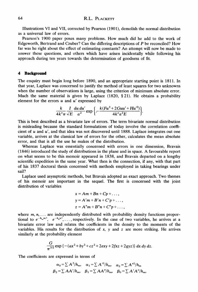
Illustrations VI and VII, corrected by Pearson (1901), demolish the normal distribution as a universal law of errors.

Pearson's 1900 paper poses many problems. How much did he add to the work of Edgeworth, Bertrand and Czuber? Can the differing descriptions of P be reconciled? How far was he right about the effect of estimating constants? An attempt will now be made to answer these questions, and others which have arisen incidentally while following his approach during ten years towards the determination of goodness of fit.

4 Background

The enquiry must begin long before 1890, and an appropriate starting point is 1811. In that year, Laplace was concerned to justify the method of least squares for two unknowns when the number of observations is large, using the criterion of minimum absolute error. Much the same material is given by Laplace (1820, ? 21). He obtains a probability element for the errors u and u' expressed by

k I dudu' k(Fu2 + 2Guu'+Hu'2) 4k" r VE a2 exp 4k"a2E

This is best described as a bivariate law of errors. The term bivariate normal distribution is misleading because the standard formulations of today involve the correlation coeffi- cient of u and u', and that idea was not discovered until 1888. Laplace integrates out one variable, arrives at the classical law of errors for the other, calculates the mean absolute error, and that is all the use he makes of the distribution.

Whereas Laplace was essentially concerned with errors in one dimension, Bravais (1846) introduced the study of distributions in the plane and in space. A favourable report on what seems to be this memoir appeared in 1838, and Bravais departed on a lengthy scientific expedition in the same year. What then is the connection, if any, with that part of his 1837 doctoral thesis concerned with methods employed in taking bearings under sail?

Laplace used asymptotic methods, but Bravais adopted an exact approach. Two themes of his memoir are important in the sequel. The first is concerned with the joint distribution of variables

x = Am +Bn +Cp+...,

y= A'm+B'n+C'p+..., z = A"m + B"n + C"p +...

where m, n, . . . are independently distributed with probability density functions propor- tional to e-h-m2, e-h-" , . . .,respectively. In the case of two variables, he arrives at a bivariate error law and relates the coefficients in the density to the moments of the variables. His results for the distribution of x, y and z are more striking. He arrives similarly at the probability element

G 3/2 exp {-(ax2+ by2 + CZ2 + 2exy +2fxz + 2gyz)} dx dy dz.

The coefficients are expressed in terms of

ao= A2Ihm, l= A'2/hm, o2=

A"2/hm

[2 = , AA'/hm, P1 =

, AA"/hm, o =

, A'A"/hm,

Karl Pearson and the chi-squared test 65

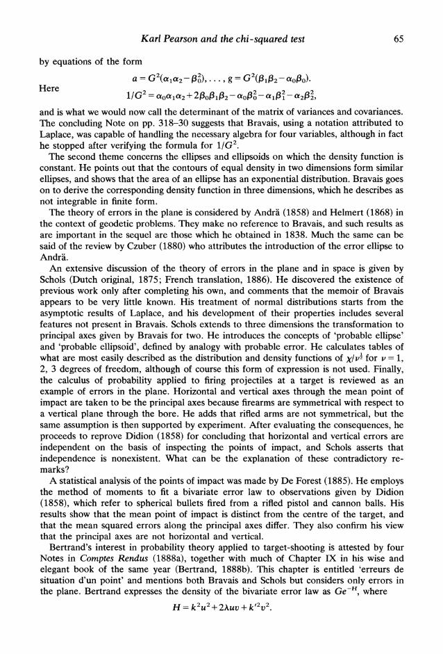
by equations of the form

a = G2 2-P),... , g = G2(p343 - ao3o). Here

1/G2 = aala2 + 22000102-ao, 1-a11 -a22,

and is what we would now call the determinant of the matrix of variances and covariances. The concluding Note on pp. 318-30 suggests that Bravais, using a notation attributed to Laplace, was capable of handling the necessary algebra for four variables, although in fact he stopped after verifying the formula for 1/G2

The second theme concerns the ellipses and ellipsoids on which the density function is constant. He points out that the contours of equal density in two dimensions form similar ellipses, and shows that the area of an ellipse has an exponential distribution. Bravais goes on to derive the corresponding density function in three dimensions, which he describes as not integrable in finite form.

The theory of errors in the plane is considered by Andri (1858) and Helmert (1868) in the context of geodetic problems. They make no reference to Bravais, and such results as are important in the sequel are those which he obtained in 1838. Much the same can be said of the review by Czuber (1880) who attributes the introduction of the error ellipse to Andra.

An extensive discussion of the theory of errors in the plane and in space is given by Schols (Dutch original, 1875; French translation, 1886). He discovered the existence of previous work only after completing his own, and comments that the memoir of Bravais appears to be very little known. His treatment of normal distributions starts from the asymptotic results of Laplace, and his development of their properties includes several features not present in Bravais. Schols extends to three dimensions the transformation to principal axes given by Bravais for two. He introduces the concepts of 'probable ellipse' and 'probable ellipsoid', defined by analogy with probable error. He calculates tables of what are most easily described as the distribution and density functions of

Xlv/ for v = 1,

2, 3 degrees of freedom, although of course this form of expression is not used. Finally, the calculus of probability applied to firing projectiles at a target is reviewed as an example of errors in the plane. Horizontal and vertical axes through the mean point of impact are taken to be the principal axes because firearms are symmetrical with respect to a vertical plane through the bore. He adds that rifled arms are not symmetrical, but the same assumption is then supported by experiment. After evaluating the consequences, he proceeds to reprove Didion (1858) for concluding that horizontal and vertical errors are independent on the basis of inspecting the points of impact, and Schols asserts that independence is nonexistent. What can be the explanation of these contradictory re- marks?

A statistical analysis of the points of impact was made by De Forest (1885). He employs the method of moments to fit a bivariate error law to observations given by Didion (1858), which refer to spherical bullets fired from a rifled pistol and cannon balls. His results show that the mean point of impact is distinct from the centre of the target, and that the mean squared errors along the principal axes differ. They also confirm his view that the principal axes are not horizontal and vertical.

Bertrand's interest in probability theory applied to target-shooting is attested by four Notes in Comptes Rendus (1888a), together with much of Chapter IX in his wise and elegant book of the same year (Bertrand, 1888b). This chapter is entitled 'erreurs de situation d'un point' and mentions both Bravais and Schols but considers only errors in the plane. Bertrand expresses the density of the bivariate error law as Ge-H, where

H= k2u 2+2Auv + k'2v)2

66 R.L. PLACKETT

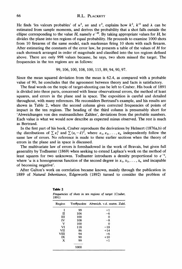
He finds 'les valeurs probables' of u2, uv and v2, explains how k2, k'2 and A can be estimated from sample moments, and derives the probability that a shot falls outside the ellipse corresponding to the value H, namely e-". By taking appropriate values for H, he divides the plane into ten regions of equal probability. He proceeds to examine 1000 shots from 10 firearms of the same model, each marksman firing 10 shots with each firearm. After estimating the constants of the error law, he presents a table of the values of H for each shotmark arranged in order of magnitude and classified into the ten regions defined above. There are only 998 values because, he says, two shots missed the target. The frequencies in the ten regions are as follows:

99, 106, 100, 108, 100, 115, 89, 94, 90, 97.

Since the mean squared deviation from the mean is 62.4, as compared with a probable value of 90, he concludes that the agreement between theory and facts is satisfactory.

The final words on the topic of target-shooting can be left to Czuber. His book of 1891 is divided into three parts, concerned with linear observational errors, the method of least squares, and errors in the plane and in space. The exposition is careful and detailed throughout, with many references. He reconsiders Bertrand's example, and his results are shown in Table 2, where the second column gives corrected frequencies of points of impact in the ten regions. The heading of the third column is presumably short for 'Abweichungen von den mutmasslichen Zahlen', deviations from the probable numbers. Each value is what we would now describe as expected minus observed. The rest is much as Bertrand.

In the first part of his book, Czuber reproduces the derivations by Helmert (1876a,b) of the distributions of E e? and E (ei _- )2, where

el, e2,..., En independently follow the

same law of errors. No reference is made to these earlier sections when the theory of errors in the plane and in space is discussed.

The multivariate law of errors is foreshadowed in the work of Bravais, but given full generality by Todhunter (1869) when seeking to extend Laplace's work on the method of least squares for two unknowns. Todhunter introduces a density proportional to e-", where 'u is a homogeneous function of the second degree in x, x2,...X , x, and incapable of becoming negative'.

After Galton's work on correlation became known, mainly through the publication in 1889 of Natural Inheritance, Edgeworth (1892) turned to consider the problem of

Table 2

Frequencies of shots in ten regions of target (Czuber, 1891)

Region Treffpunkte Abweich. v.d. mutm. Zahl.

I 99 +1 II 106 -6

III 100 0 IV 108 -8 V 100 0

VI 118 -18 VII 86 +14

VIII 94 +6 IX 90 +10 X 99 +1

1000

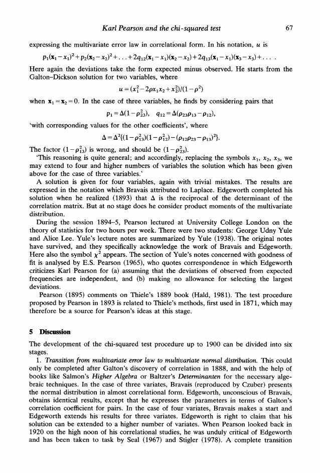
Karl Pearson and the chi-squared test 67

expressing the multivariate error law in correlational form. In his notation, u is

pl(xl- Xl)2

+ p2(x2- x2)2+... + 2q12(x1- x1)(X2 - 2)+ 2q13(x1- X1)(X3- x3) + ....

Here again the deviations take the form expected minus observed. He starts from the Galton-Dickson solution for two variables, where

u = (X2- 2px12 + )/(1 - 2)

when x, = X2 = 0. In the case of three variables, he finds by considering pairs that

p= A(1 - P~23), q12 = A(P23P13 -P12),

'with corresponding values for the other coefficients', where

A = A2{(1 - P13)( - P 12) - (12P23 - P13)2}?

The factor (1- p13) is wrong, and should be (1- p23). 'This reasoning is quite general; and accordingly, replacing the symbols x1, x2, x3, we

may extend to four and higher numbers of variables the solution which has been given above for the case of three variables.'

A solution is given for four variables, again with trivial mistakes. The results are expressed in the notation which Bravais attributed to Laplace. Edgeworth completed his solution when he realized (1893) that A is the reciprocal of the determinant of the correlation matrix. But at no stage does he consider product moments of the multivariate distribution.

During the session 1894-5, Pearson lectured at University College London on the theory of statistics for two hours per week. There were two students: George Udny Yule and Alice Lee. Yule's lecture notes are summarized by Yule (1938). The original notes have survived, and they specifically acknowledge the work of Bravais and Edgeworth. Here also the symbol X2 appears. The section of Yule's notes concerned with goodness of fit is analysed by E.S. Pearson (1965), who quotes correspondence in which Edgeworth criticizes Karl Pearson for (a) assuming that the deviations of observed from expected frequencies are independent, and (b) making no allowance for selecting the largest deviations.

Pearson (1895) comments on Thiele's 1889 book (Hald, 1981). The test procedure proposed by Pearson in 1893 is related to Thiele's methods, first used in 1871, which may therefore be a source for Pearson's ideas at this stage.

5 Discussion

The development of the chi-squared test procedure up to 1900 can be divided into six stages.

1. Transition from multivariate error law to multivariate normal distribution. This could only be completed after Galton's discovery of correlation in 1888, and with the help of books like Salmon's Higher Algebra or Baltzer's Determinanten for the necessary alge- braic techniques. In the case of three variates, Bravais (reproduced by Czuber) presents the normal distribution in almost correlational form. Edgeworth, unconscious of Bravais, obtains identical results, except that he expresses the parameters in terms of Galton's correlation coefficient for pairs. In the case of four variates, Bravais makes a start and Edgeworth extends his results for three variates. Edgeworth is right to claim that his solution can be extended to a higher number of variates. When Pearson looked back in 1920 on the high noon of his correlational studies, he was unduly critical of Edgeworth and has been taken to task by Seal (1967) and Stigler (1978). A complete transition

68 R.L. PLACKETT

awaited the product-moment definition of correlation coefficient (Pearson, 1896), but Edgeworth's theorem is justly named.

2. Distribution of exponent in multivariate normal density. The methodical Czuber did not appreciate that the results of Bravais and Schols had a common structure with the distributions obtained by Helmert in a different context. Pearson was even less likely to do so when he extended these results from 2 and 3 variates to any number.

'The field was very wide and I was far too excited to stop to investigate properly what other people had done. I wanted to reach new results and apply them.'

Thus wrote Pearson in 1920. Later in the decade his historical studies led him back to Czuber and he reproduced Helmert's work (Pearson, 1931). Since then the frontiers of discovery have been pushed further back. The distribution of 8CE was derived before 1876, in effect by Bienaym6 (1852), who also obtained the series expansions used by Pearson, and in actuality by Abbe (1863, collected works 1906), as pointed out by Lancaster (1966) and Sheynin (1966) respectively. However, their description of 8 e? as X2 can be faulted for two reasons. First, while acknowledging the level of intellectual attainment represented by derivations before Pearson, the fact is that all these earlier results had no impact on the progress of mainstream statistics. Secondly, X2 is not only a distribution, but also a statistic and a test procedure, all of which arrived simultaneously. Lancaster finds in the paper by Bienaym6 (1838) a quantity similar to Pearson's statistic, and attributes to him a central limit theorem for the multinomial distribution, but these conclusions are disputed by Heyde & Seneta (1977, p. 102).

3. Approximation of multinomial distribution by multivariate normal density. Pearson gives no explanation in 1900, but his argument can be inferred from subsequent papers, for example Pearson (1916a), which show him to be assuming that individual normality implies joint normality, as noted by Lancaster (1969, 1972). Pearson still believed this argument in 1934.

When preparing his lectures on the history of statistics in the 17th and 18th centuries, Pearson discovered around 1927 that Lagrange had by 1776 derived the multivariate error law as an approximation to the multinomial distribution. The lecture notes (edited by E.S. Pearson, 1978) describe the 'volume' outside an ellipsoid in multiple space as 'the chance that the probability shall exceed a given value P'. This sheds some light on his 1900 phrase 'as great or greater frequency than that denoted by X'.

Another discovery of the approximation is noted by MacKenzie (1977, 1981). When did the extension of De Moivre's theorem from the binomial to the multinomial distribu- tion become an established result?

4. Evaluation of exponent when moments are those of multinomial. Pearson the applied mathematician whould have no difficulty with moments. He had more trouble in evaluat- ing X2 for deviations which sum to zero. This is the longest piece of algebra in the paper, suggesting a discovery more recent than that of the distribution of X2, which occupies only 16 lines.

5. Definition of the event to which the probability P refers. There are two equivalent interpretations of Pearson's description: (a) deviations from expected as large or larger than observed; (b) probability density as small or smaller than observed. Were both intended? If only one, then which one?

The title of the 1900 paper refers to 'deviations from the probable' and illustration IV to 'deviations... from the most probable'. A comparison with the terminology used by

Karl Pearson and the chi-squared test 69

Bertrand and Czuber, and by Pearson himself in 1893, shows that this phrase means deviations from the expected value.

The initial description of P concerns 'a system of errors with as great or greater frequency than that denoted by X' and comes immediately after a reference to the ellipsoid of constant frequency. This ellipsoid, considered theoretically by Bravais and Schols, and observed in practice by Galton (1889, p. 101), was the foundation stone of multiple correlation, and therefore a concept which Pearson would mention quite natur- ally. Yule's notes of 1895 refer to 'the ellipse X' and 'the ellipsoid X'. Thus X identifies the ellipsoid with constant frequency, and values of X are implied by the term 'as great or greater frequency'.

Illustration II refers to 'a system of deviations as improbable or more improbable than this one'. Such a definition accords with the idea of frequencies as small or smaller, although Pearson never uses that phrase. Furthermore, the definition is vague and could equally be used when applying a t test, for example.

Consequently, interpretation (a) is preferred here, whereas Cox & Hinkley (1978, problem 3.3) favour (b), and Chang (1973) proposes a version which combines (a) and (b). A clear statement of (b) is given by Neyman & E.S. Pearson (1928, p. 183).

6. Allowance for the effect of estimating unknown parameters. Virtually all the work on this problem postdates Pearson (1900) and only a few brief comments can be made here. The current orthodox view is that established by Fisher in the 1920's using the concept of 'degrees of freedom', a number which is reduced by one for each parameter efficiently estimated. Bartlett (1981, p. 6) quotes from a letter of E.S. Pearson dated 30 March 1979:

'I knew long ago that KP used the 'correct' degrees of freedom for (a) difference between two samples and (b) multiple contingency tables. But he could not see that X2 in curve fitting should be got asymptotically into the same category.'

Here Pearson (1916b) is relevant. In an unpublished Fisher memorial lecture, G.A. Barnard makes a distinction between types of parameter which affects the calculation of the degrees of freedom.

6 Conclusions

When Pearson began his statistical career, the problem of assessing whether or not standard distributions provided acceptable fits to sets of data was well known. Simple tests using normal approximations to binomial distributions were introduced by Laplace, and comparisons of statistics with their expected values had taken over from subjective inspections of a set of frequencies. Pearson's attention was immediately directed to the problem when he added to the existing corpus of artificial experiments. Within two years he was able to produce a test procedure based on 'the standard deviation of the standard deviation' which represented an advance on anything else accessible in 1893. After that, the problem of goodness of fit marked time while correlation and regression were vigorously pushed forward and the range of standard distributions was extended by the Pearson system. Nothing of importance to the problem appears in his published work during this period although further exploration evidently rumbled on in lecture notes and correspondence.

In the 1900 paper, Pearson confronted all the difficulties. They are concerned with distribution theory, asymptotic approximations, singular matrices, and the effect of estimating parameters. Edgeworth had already expressed the multivariate normal dis- tribution in operational form. Pearson proceeded to give the distribution theory of the exponent in full generality, derive a simple and appropriate test statistic, and press on to

70 R.L. PLACKETT

the applications with all that they implied for the status of the law of errors. Some theoretical details are omitted and he has been particularly criticized for mistaking the effects of estimation. The faults of the paper may be explained either by the excitement which Pearson recalled in 1920, or by other aspects of his personality, for which see Greenwood (1949) and Yule (1936). However, the surprising thing is not that the paper has faults, but that so much was accomplished. Furthermore, Pearson inaugurated lines of research in many fields which are still active, for example goodness of fit, contingency tables, and measures of association.

The many positive aspects of originality and usefulness far outweigh the defects of presentation. Pearson's 1900 paper on chi squared is one of the great monuments of twentieth century statistics.

Acknowledgements

I am grateful to Professor S.M. Stigler for comments on an earlier draft, Professor M. Stone for a copy of the relevant pages of Yule's lecture notes, Dr Anne Dickinson for the resume and the referee for informed criticisms.

References

Abbe, E. (1906). Uber die Gesetzmissigkeit der Vertheilung der Fehler bei Beobachtungsreihen. Gesammelte Abhandlungen 2, 55-81.

Andri, C.G. (1858). Fehlerbestimmung bei der Auflosung der Pothenot'schen Aufgabe mit dem Messtische. Astron. Nach. 47, col 193-202.

Bartlett, M.S. (1981). Egon Sharpe Pearson, 1895-1980. Biometrika 68, 1-7. Bertrand, J. (1888a). Probabilit6 du tir a la cible. Comptes Rendus 106, 232-234, 387-392, 521-522; 107,

205-207. Bertrand, J. (1888b). Calcul des Probabilitis. Paris: Gauthier-Villars. Bienaym6, J. (1838). Sur la probabilit6 des r6sultats moyens des observations: demonstration directe de la regle

de Laplace. Mgm. pres. Acad. Roy. Sci. Inst. France 5, 513-558. Bienaym6, J. (1852). Sur la probabilit6 des erreurs d'apres la m6thode des moindres carr6s. Liouville's J. Math.

Pures Appl. (1) 17, 33-78. Bravais, A. (1838). (Rapport sur ce M6moire). Comptes Rendus 7, 77-78. Bravais, A. (1846). Analyse math6matique sur les probabilit6s des erreurs de situation d'un point. Mgm. pros.

Acad. Roy. Sci. Inst. France 9, 255-332. Chang, W-C. (1973). A History of the Chi-Square Goodness-of-Fit Test. PhD thesis, University of Toronto. Cox, D.R. & Hinkley, D.V. (1978). Problems and Solutions in Theoretical Statistics. London: Chapman & Hall. Czuber, E. (1880). Zur Theorie der Fehlerellipse. Sitz-Ber. Math Naturwissenschaftliche Cl. Kais. Akad. Wiss.

Wien 82, 698-723. Czuber, E. (1891). Theorie der Beobachtungsfehler. Leipzig: Teubner. De Forest, E.L. (1885). On the law of error in target-shooting. Trans. Connecticut Acad. Art. Sci. 7, 1-8. Dickson, J.D.H. (1889). Appendix B in Galton (1889). Didion, I. (1858). Calcul des Probabilitis applique au Tir des Projectiles. Paris. Edgeworth, F.Y. (1892). Correlated averages. Phil. Mag. (5) 34, 190-204. Edgeworth, F.Y. (1893). Note on the calculation of correlation between organs. Phil. Mag. (5) 36, 350-351. Fisher, R.A. (1922). On the interpretation of chi square from contingency tables, and the calculation of P. J.R.

Statist. Soc. 85, 87-94. Fisher, R.A. (1923). Statistical tests of agreement between observation and hypothesis. Economica 8, 1-9. Fisher, R.A. (1924). The conditions under which chi square measures the discrepancy between observation and

hypothesis. J.R. Statist. Soc. 57, 442-450. Fisher, R.A. (1925). Statistical Methods for Research Workers. Edinburgh: Oliver & Boyd. Galton, F. (1889). Natural Inheritance. London: Macmillan. Greenwood, M. (1949). Karl Pearson. In Dictionary of National Biography, 1931-40, pp. 681-684. Oxford

University Press. Hald, A. (1981). T.N. Thiele's contributions to statistics. Int. Statist. Rev. 49, 1-20. Helmert, F.R. (1868). Studien iiber rationelle Vermessungen im Gebiete der hihern Geodisie. Zeit. f. Math. u.

Phys. 13, 73-120. Helmert, F.R. (1876a). Ober die Wahrscheinlichkeit der Potenzsummen der Beobachtungsfehler und iiber einige

damit im Zusammenhange stehende Fragen. Zeit. f. Math. u. Phys. 21, 192-218. Helmert, F.R. (1876b). Die Genauigkeit der Formel von Peters zur Berechnung des wahrscheinlichen Beobach-

tungsfehlers directer Beobachtungen gleicher Genauigkeit. Astron. Nach. 88, col 113-132.

Karl Pearson and the chi-squared test 71

Heyde, C.C. & Seneta, E. (1977). I.J. Bienayme: Statistical Theory Anticipated. New York: Springer. Kendall, M. & Plackett, R.L. (Eds.). (1977). Studies in the History of Statistics and Probability, 2. London:

Griffin. Lagrange, J.L. (1776). M6moire sur l'utilit6 de la methode de prendre le milieu entres les resultats de plusieurs

observations, dans lequel on examine les avantages de cette methode par le calcul des probabilites, et oii l'on resout diff6rents problemes relatifs a cette matiere. Miscellanea Taurinensia 5; (1868) OEuvres 2, 173-234.

Lancaster, H.O. (1966). Forerunners of the Pearson X2. Aust. J. Statist. 8, 117-26. Lancaster, H.O. (1969). The Chi-squared Distribution. New York: Wiley. Lancaster, H.O. (1972). Development of the notion of statistical dependence. Math. Chronicle (NZ) 2, 1-16.

Reprinted in Kendall & Plackett (1977), pp. 293-308. Laplace, P.S. (1811). Memoire sur les integrales definies, et leur application aux probabilites, et specialement a

la recherche du milieu qu'il faut choisir entre les resultats des observations. Mgm. Inst. Imp. France Annie 1810, pp. 279-347.

Laplace, P.S. (1820). Theorie Analytique des Probabilitis, 3rd edition; (1886) OEuvres 7; Paris. Lenin, V.I. (1970). Materialism and Empirio-Criticism: Critical Comments on a Reactionary Philosophy.

Moscow: Progress. MacKenzie, D. (1977). Studies in the History of Probability and Statistics. XXXVI. Arthur Black: A forgotten

pioneer of mathematical statistics. Biometrika 64, 613-616. MacKenzie, D.A. (1981). Statistics in Britain 1865-1930. The Social Construction of Scientific Knowledge.

Edinburgh University Press. Neyman, J. & Pearson, E.S. (1928). On the use and interpretation of certain test criteria for purposes of

statistical inference. Parts I, II. Biometrika 20A, 175-240, 263-294. Pearson, E.S. (1938). Karl Pearson: An Appreciation of Some Aspects of his Life and Work. Cambridge

University Press. Pearson, E.S. (1965). Some incidents in the early history of biometry and statistics 1890-94. Biometrika 52,

3-18. Reprinted in Pearson & Kendall (1970), pp. 323-338. Pearson, E.S. & Kendall, M.G. (Eds.). (1970). Studies in the History of Statistics and Probability. London:

Griffin. Pearson, K. (1894). Science and Monte Carlo. The Fortnightly Review, new series, 55, 183-193. Pearson, K. (1895). Contributions to the mathematical theory of evolution, II. Skew variation in homogeneous

material. Phil. Trans. A 186, 343-414. Reprinted in K. Pearson (1956), pp. 41-112. Pearson, K. (1896). Mathematical contributions to the theory of evolution, III. Regression, heredity and

panmixia. Phil. Trans. A 187, 253-318. Reprinted in K. Pearson (1956), pp. 113-178. Pearson, K. (1897a). The Chances of Death and Other Studies in Evolution, 2 vols. London: Edward Arnold. Pearson, K. (1897b). Cloudiness: note on a novel case of frequency. Proc. R. Soc. Lond. 62, 287-290. Pearson, K. (1900). On the criterion that a given system of deviations from the probable in the case of a

correlated system of variables is such that it can be reasonably supposed to have arisen from random sampling. Phil. Mag. (5) 50, 157-175. Reprinted in K. Pearson (1956), pp. 339-357.

Pearson, K. (1901). The normal curve of errors. Phil. Mag. (6) 1, 670-1. Pearson, K. (1916a). On a brief proof of the fundamental formula for testing the goodness of fit of frequency

distributions and on the probable error of 'P'. Phil. Mag. (6) 31, 369-378. Pearson, K. (1916b). On the general theory of multiple contingency with special reference to partial contingency.

Biometrika 11, 145-158. Pearson, K. (1920). Notes on the history of correlation. Biometrika 13, 25-45. Reprinted in E.S. Pearson &

Kendall (1970), pp. 185-205. Pearson, K. (1931). Historical note on the distribution of the standard deviations of samples of any size drawn

from an indefinitely large normal parent population. Biometrika 23, 416-418. Pearson, K. (1934). On a new method of determining 'goodness of fit'. Biometrika 26, 425-442. Pearson, K. (1956). Karl Pearson's Early Statistical Papers. Cambridge University Press. Pearson, K. (Ed. E.S. Pearson) (1978). The History of Statistics in the 17th and 18th Centuries against the

Changing Background of Intellectual, Scientific and Religious Thought. London: Griffin. Schols, C.M. (1875). Over de theorie der fouten in de ruimte en in het platte vlak. Verh. Nederl. Akad.

Wetensch. 15, 1-75. Schols, C.M. (1886). Th6orie des erreurs dans le plan et dans l'espace. Annales de l'Ecole Polytechnique de Delft

2, 123-179. Seal, H.L. (1967). The historical development of the Gauss linear model. Biometrika 54, 1-24. Reprinted in E.S.

Pearson & Kendall (1970), pp. 207-230. Sheynin, O.B. (1966). Origin of the theory of errors. Nature 211, 1003-1004. Stigler, S.M. (1978). Francis Ysidro Edgeworth, statistician (with discussion). J.R. Statist. Soc. A 141, 287-322. Todhunter, I. (1869). On the method of least squares. Trans. Camb. Phil. Soc. 11, 219-238. Yule, G.U. (1897). Note on the teaching of the theory of statistics at University College. J.R. Statist. Soc. 60,

456-458. Yule, G.U. (1936). Karl Pearson 1857-1936. Obituary Notices of Fellows of the Royal Society of London 2,

73-104. Yule, G.U. (1938). Notes of Karl Pearson's lectures on the theory of statistics, 1894-96. Biometrika 30,

198-203.

72 R.L. PLACKETr

R&sume

La communication de Pearson en 1900 pr6sentait ce que ulterieurement est devenu l'6preuve de Chi-carr6 d'excellence d'ajustement. La terminologie et les allusions d'il y a quatre-vingt ans cr6ent une barriere pour le lecteur moderne, qui trouve que l'interpretation du procedure de l'6preuve de Pearson et la d6termination de ce qu'il a achev6 ne sont pas trbs nettes en d6pit des avances techniques qui ont 6t6 faites depuis lors. Ici j'ai fait un effort de surmonter ces difficult6s par les moyens de l'exploration des activit6s pertinantes de Pearson pendant la premiere d6cade de sa carriere en statistiques, et de la description du travail de ses contemporains et

pr6d6cesseurs qui semble avoir eu une influence sur son approche au probleme. Je n'ai pas eu une r6ponse e toutes les questions, et il y en a d'autres qui resteront pour une etude ulterieure.

[Paper received March 1982, revised August 1982]