K.7

Scarred Consumption Malmendier, Ulrike and Leslie Sheng Shen

International Finance Discussion Papers Board of Governors of the Federal Reserve System

Number 1259 October 2019

Please cite paper as: Malmendier, Ulrike and Leslie Sheng Shen (2019). Scarred Consumption. International Finance Discussion Papers 1259. https://doi.org/10.17016/IFDP.2019.1259

Board of Governors of the Federal Reserve System

International Finance Discussion Papers

Number 1259

October 2019

Scarred Consumption

Ulrike Malmendier and Leslie Sheng Shen

NOTE: International Finance Discussion Papers are preliminary materials circulated to stimulate discussion and critical comment. References to International Finance Discussion Papers (other than an acknowledgment that the writer has had access to unpublished material) should be cleared with the author or authors. Recent IFDPs are available on the Web at www.federalreserve.gov/pubs/ifdp/. This paper can be downloaded without charge from the Social Science Research Network electronic library at www.ssrn.com.

Scarred Consumption

Ulrike Malmendiera,c,d and Leslie Sheng Shenb

Abstract: We show that prior lifetime experiences can “scar” consumers. Consumers who have lived through times of high unemployment exhibit persistent pessimism about their future financial situation and spend significantly less, controlling for the standard life-cycle consumption factors, even though their actual future income is uncorrelated with past experiences. Due to their experience-induced frugality, scarred consumers build up more wealth. We use a stochastic life-cycle model to show that the negative relationship between past experiences and consumption cannot be generated by financial constraints, income scarring, and unemployment scarring, but is consistent with experience-based learning.

Keywords: Household consumption, experience effects, expectation, lifecycle model

JEL classifications: D12, D15, D83, D91, G51

* a University of California at Berkeley; b Federal Reserve Board; c NBER; d CEPR. We thank JohnBeshears, David Card, Alex Chinco, Ed Glaeser, Yuriy Gorodnichenko, Pierre-Olivier Gourinchas, Pat Kline, David Laibson, Jonathan Parker, Luigi Pistaferri, Joseph Vavra and seminar participants at Bocconi University, IZA/University of Bonn, MIT, Stanford University, UC Berkeley (Macro, Labor, Finance), University of Minnesota, University of Tilburg, University of Zurich, NBER SI (EFBEM, EFG-PD), the SITE workshop, Conference in Behavioral Finance and Decision Making, the CESifo Area Conference on Behavioral Economics, the Cleveland Fed Household Economics and Decision Making Conference, and 2016 EWEBE Conference in Cologne for helpful comments, and Clint Hamilton, Canyao Liu, and Ian Chin for excellent research assistance. The views in this paper are solely the responsibility of the author(s) and should not be interpreted as reflecting the views of the Board of Governors of the Federal Reserve System or of any other person associated with the Federal Reserve System.

The crisis has left deep scars, which will a↵ect both supply and demand

for many years to come. — Blanchard (2012)

I Introduction

More than a decade after the Great Recession, consumers have been slow to return

to prior consumption levels (Petev et al. 2011, De Nardi et al. 2012). As the

quote above suggests, the crisis appears to have “scarred” consumers. Consumption

has remained low not only in absolute levels, but also relative to the growth of

income, net worth, and employment—a pattern that challenges standard life-cycle

consumption explanations, such as time-varying financial constraints. For the same

reason, low employment due to the loss of worker skills or low private investment,

as put forward in the literature on “secular stagnation” and “hysteresis,” cannot

account for the empirical pattern either.1

What, then, explains such long-term e↵ects of a macroeconomic crisis on con-

sumption? Our hypothesis starts from the observation in Pistaferri (2016) that the

long-lasting crisis e↵ects are accompanied by consumer confidence remaining low for

longer periods than standard models imply. We relate this observation to the notion

of experience-based learning. We show that consumers’ past lifetime experiences of

economic conditions have a long-lasting e↵ect on beliefs and consumption, which is

not explained by income, wealth, liquidity, and other life-cycle determinants.

Prior research on experience e↵ects has shown that personally experienced stock-

market and inflation realizations receive extra weight when individuals form expec-

tations about future realizations of the same variables.2 Here, we ask whether a

similar mechanism is at work when individuals experience high unemployment rates.

We apply the linearly declining weights estimated in prior work to both national and

1 The literature on secular stagnation conjectured protracted times of low growth after the GreatDepression (Hansen 1939). Researchers have applied the concept to explain scarring e↵ects of theGreat Recession (Delong and Summers 2012, Summers 2014a, 2014b). Blanchard and Summers(1986) introduce the term “hysteresis e↵ects” to characterize the high and rising unemployment inEurope. Cf. Cerra and Saxena (2008), Reinhart and Rogo↵ (2009), Ball (2014), Haltmaier (2012),and Reifschneider, Wascher, and Wilcox (2015).

2 Theoretical papers on the macro e↵ects of learning-from-experience in OLG models includeEhling, Graniero, and Heyerdahl-Larsen (2018), Malmendier, Pouzo, and Vanasco (2018), Collin-Dufresne, Johannes, and Lochstoer (2016), and Schraeder (2015). The empirical literature startsfrom Kaustia and Knupfer (2008) and Malmendier and Nagel (2011, 2015).

1

local unemployment rates that individuals have experienced over their lives so far,

and to their personal unemployment experiences. We show that past experiences

predict both consumer pessimism (beliefs) and consumption scarring (expenditures)

as well as several other empirical regularities, including generational di↵erences in

consumption patterns, after controlling for wealth, income and other standard de-

terminants. At the same time, past experiences do not predict future income, after

including the same controls, and predict, if anything a positive wealth build up.

We start by presenting four baseline findings on the relation between past ex-

periences and consumption, beliefs, future income, and wealth build-up. We first

document the long-lasting e↵ect of past experiences on consumption. Using the

Panel Study of Income Dynamics (PSID) from 1999-2013, we find that past macro

and personal unemployment experiences have significant predictive power for con-

sumption, controlling for income, wealth, age fixed e↵ects, a broad range of other

demographic controls (including current unemployment), as well as state, year, and

even household fixed e↵ects. To the best of our knowledge, our analysis is the first to

estimate experience e↵ects also within household, i. e., controlling for any unspeci-

fied household characteristics. Without household dummies, the identification comes

both from cross-household di↵erences in consumption and unemployment histories,

and from how these di↵erences vary over time. With household dummies, the es-

timation relies solely on within-household variation in consumption in response to

lifetime experiences.3 In both cases, the e↵ects are sizable. A one standard devi-

ation increase in the macro-level measure is associated with a 3.3% ($279) decline

in annual food consumption, and a 1.6% ($713) decline in total consumption. A

one standard deviation increase in personal unemployment experiences is associated

with 3.7% ($314) and 2.1% ($937) decreases in annual spending on food and total

consumption, respectively. The results are robust to variations in accounting for the

spouse’s experience, excluding last year’s experience, or using di↵erent weights, from

3 We have also estimated a model with cohort fixed e↵ects. In that case, the identificationcontrols for cohort-specific di↵erences in consumption. The results are very similar to estimationswithout cohort fixed e↵ects. Note that, di↵erently from most of the prior literature on experiencee↵ects (Malmendier and Nagel 2011, 2015), the experience measure is not absorbed by cohort fixede↵ects as the consumption data sets contain substantial within-cohort variation in experiences. Theunemployment experience measure of a given cohort varies over time depending on where the cohortmembers have resided over their prior lifetimes.

2

equal to steeper-than-linearly declining.4

Second, we document that consumers’ past experiences significantly a↵ect beliefs.

Using the Michigan Survey of Consumers (MSC) from 1953 to 2013, we show that

people who have experienced higher unemployment rates over their lifetimes so far

have more pessimistic beliefs about their financial situation in the future, and are

more likely to believe that it is not a good time to purchase major household items

in general. Importantly, these estimations control for income, age, time e↵ects, and

a host of demographic and market controls.

Third, we relate the same measure of lifetime unemployment experiences to actual

future income, up to three PSID waves (six years) in the future. Again, we control for

current income, wealth, demographics, as well as age, state, year, and even household

fixed e↵ects. We fail to identify any robust relation. In other words, while there is

a strong reaction to prior lifetime experiences in terms of beliefs and consumption

expenditures, actual future income does not appear to explain these adjustments.

Our fourth baseline result captures the wealth implications of consumption scar-

ring. If consumers become more frugal in their spending after negative past experi-

ences, even though they do not earn a reduced income, we would expect their savings

and ultimately their wealth to increase. Our fourth finding confirms this prediction

in the data. Using a horizon of three to seven PSID waves (6 to 14 years), we find

past lifetime experiences predict liquid and illiquid wealth build up, in particular

for past personal unemployment experiences. Unobserved wealth e↵ects, the main

alternative hypothesis, do not predict wealth build up, or even predict the opposite.

These four baseline results—a lasting influence of economic experiences in the

past on current expenditure decisions and on consumer optimism, but the lack of

any e↵ect on actual future income, plus positive wealth build-up—are consistent

with our hypothesis: Consumers over-weigh experiences they made during their

prior lifetimes when forming beliefs about future realizations and making consump-

tion choices, as predicted by models of experience-based learning (EBL). Considered

jointly, and given the controls included in the econometric models, the results so

far already distinguish our hypothesis from several alternative explanations: The

inclusion of age controls rules out certain life-cycle e↵ects, such as an increase in

4 We also included lagged consumption in the estimation model to capture habit formation butdo not find a significant e↵ect, while the experience proxy remains significant.

3

precautionary motives and risk aversion with age (cf. Caballero 1990, Carroll 1994),

or declining income and tighter liquidity constraints during retirement (cf. Deaton

1991, Gourinchas and Parker 2002). The controls for labor market status and demo-

graphics account for intertemporal expenditure allocation as in Blundell, Browning,

and Meghir (1994) or Attanasio and Browning (1995). The time fixed e↵ects control

for common shocks and available information such as the current and past national

unemployment rates. The PSID also has the advantage of containing information on

wealth, a key variable in consumption models. Moreover, the panel structure of the

PSID data allows for the inclusion of household fixed e↵ects and thus to control for

time-invariant unobserved heterogeneity.

To further distinguish EBL from other determinants that can be embedded in

a life-cycle permanent-income model, we simulate the Low, Meghir, and Pistaferri

(2010) model of consumption and labor supply and use estimations on the simulated

data to illustrate directional di↵erences and other distinctive e↵ects. The Low et al.

(2010) model accounts for various types of shocks, including productivity and job

arrival, and allows for financial constraints as well as “income scarring”—the notion

that job loss may have long-lasting e↵ects on future income because it takes time

to obtain an o↵er of the same job-match quality as before unemployment. We fur-

ther extend the Low et al. (2010) model to allow for “unemployment scarring”—the

notion that job loss itself may induce a negative, permanent wage shock.5 We con-

trast these explanations with EBL by simulating the model for both Bayesian and

experience-based learners.

First, we utilize the simulations to show that, even with all of the life-cycle

determinants and frictions built into the Low et al. model, it is hard to generate

a negative correlation between past unemployment experiences and consumption

when consumers are rational, after controlling for income and wealth. This holds

both when we allow for financial constraints and income scarring, as in Low et al.,

and when we further add unemployment scarring. In fact, given the income control,

the simulate-and-estimate exercise often predicts a positive relation between unem-

ployment experiences and consumption. Intuitively, a consumer who has the same

income as another consumer despite worse unemployment experiences likely has a

higher permanent income component, and rationally consumes more.

5 We thank the audience at the University of Minnesota macro seminar for this useful suggestion.

4

We then turn to consumers who overweight their own past experiences when

forming beliefs. Here, we find the opposite e↵ect: Higher life-time unemployment

experiences predict lower consumption among EBL agents, controlling for income

and wealth. Thus, the simulate-and-estimate exercise disentangles EBL from po-

tential confounds such as financial constraints, income scarring, and unemployment

scarring. There is a robust negative relation between past experiences and consump-

tion under EBL, consistent with the empirical estimates, but not under Bayesian

learning. Moreover, Bayesian learning is inconsistent with the estimated relation

between past experiences and downward biased beliefs.

The model also helps to alleviate concerns about imperfect wealth controls. We

conduct both simulate-and-estimate exercises leaving out the wealth control in the

estimation. In the case of rational consumers we continue to estimate a positive

rather than negative relationship between past experiences and consumption; in the

case of experience-base learners, we continue to estimate a negative relationship.

Guided by these simulation results, we perform three more empirical steps: (1)

a broad range of robustness checks and replications using variations in the wealth,

liquidity, and income controls, and using di↵erent data sets; (2) a study of the impli-

cations of EBL for the quality of consumption and of the heterogeneity in consump-

tion patterns across cohorts, and (3) a discussion of the potential aggregate e↵ects

of EBL for consumption and savings.

First, we replicate the PSID results using four variants of wealth controls: third-

and fourth-order liquid and illiquid wealth; decile dummies of liquid and illiquid

wealth; separate controls for housing and other wealth; and controls for positive

wealth and debt. Similarly, we check the robustness to four variants of the income

controls: third- and fourth-order income and lagged income; quintile dummies of

income and lagged income; decile dummies of income and lagged income; and five

separate dummies for two-percentile steps in the bottom and in the top 10% of income

and lagged income. All variants are included in addition to first- and second-order

liquid and illiquid wealth and first- and second-order income and lagged income, and

all estimations are replicated both with and without household fixed e↵ects. We

also subsample households with low versus high liquid wealth (relative to the sample

median in a given year), and find experience e↵ects in both subsamples.6

6 Our variants of wealth and income controls also address the concern that consumption may

5

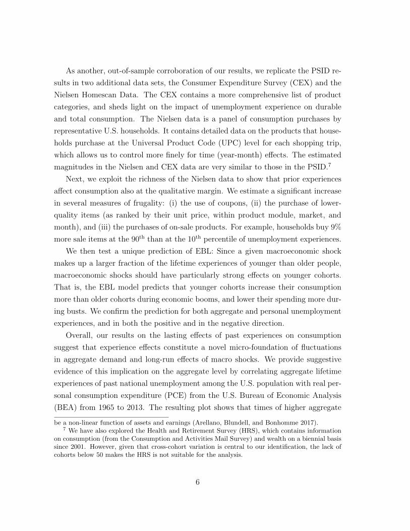
As another, out-of-sample corroboration of our results, we replicate the PSID re-

sults in two additional data sets, the Consumer Expenditure Survey (CEX) and the

Nielsen Homescan Data. The CEX contains a more comprehensive list of product

categories, and sheds light on the impact of unemployment experience on durable

and total consumption. The Nielsen data is a panel of consumption purchases by

representative U.S. households. It contains detailed data on the products that house-

holds purchase at the Universal Product Code (UPC) level for each shopping trip,

which allows us to control more finely for time (year-month) e↵ects. The estimated

magnitudes in the Nielsen and CEX data are very similar to those in the PSID.7

Next, we exploit the richness of the Nielsen data to show that prior experiences

a↵ect consumption also at the qualitative margin. We estimate a significant increase

in several measures of frugality: (i) the use of coupons, (ii) the purchase of lower-

quality items (as ranked by their unit price, within product module, market, and

month), and (iii) the purchases of on-sale products. For example, households buy 9%

more sale items at the 90th than at the 10th percentile of unemployment experiences.

We then test a unique prediction of EBL: Since a given macroeconomic shock

makes up a larger fraction of the lifetime experiences of younger than older people,

macroeconomic shocks should have particularly strong e↵ects on younger cohorts.

That is, the EBL model predicts that younger cohorts increase their consumption

more than older cohorts during economic booms, and lower their spending more dur-

ing busts. We confirm the prediction for both aggregate and personal unemployment

experiences, and in both the positive and in the negative direction.

Overall, our results on the lasting e↵ects of past experiences on consumption

suggest that experience e↵ects constitute a novel micro-foundation of fluctuations

in aggregate demand and long-run e↵ects of macro shocks. We provide suggestive

evidence of this implication on the aggregate level by correlating aggregate lifetime

experiences of past national unemployment among the U.S. population with real per-

sonal consumption expenditure (PCE) from the U.S. Bureau of Economic Analysis

(BEA) from 1965 to 2013. The resulting plot shows that times of higher aggregate

be a non-linear function of assets and earnings (Arellano, Blundell, and Bonhomme 2017).7 We have also explored the Health and Retirement Survey (HRS), which contains information

on consumption (from the Consumption and Activities Mail Survey) and wealth on a biennial basissince 2001. However, given that cross-cohort variation is central to our identification, the lack ofcohorts below 50 makes the HRS is not suitable for the analysis.

6

past-unemployment experience in the population coincide with lower aggregate con-

sumer spending. This suggests that changes in aggregate consumption may reflect

not only responses to recent labor-market adjustments, but also changes in belief for-

mation due to personal lifetime experiences of economic shocks. Overall, our findings

imply that the long-term consequences of macroeconomic fluctuations can be signif-

icant, thus calling for more discussion on optimal monetary and fiscal stabilization

policy to control unemployment and inflation (Woodford 2003, 2010).

Related Literature Our work connects several strands of literature.

First and foremost, the paper contributes to a rich literature on consumption.

Since the seminal work of Modigliani and Brumberg (1954) and Friedman (1957),

the life-cycle permanent-income model has been the workhorse to study consump-

tion behavior. Consumption decisions are an intertemporal allocation problem, and

agents smooth marginal utility of wealth across predictable income changes over

their life-cycle. Subsequent variants provide more rigorous treatments of uncertainty,

time-separability, and the curvature of the utility function (see Deaton (1992) and

Attanasio (1999) for overviews). A number of empirical findings, however, remain

hard to reconcile with the model predictions. Campbell and Deaton (1989) point out

that consumption does not react su�ciently to unanticipated innovation to the per-

manent component of income (excess smoothness). Instead, consumption responds

to anticipated income increases, over and above what is implied by standard models

of consumption smoothing (excess sensitivity; cf. West 1989, Flavin 1993).

The empirical puzzles have given rise to a debate about additional determinants

of consumption, ranging from traditional explanations such as liquidity constraints

(Gourinchas and Parker 2002; see also Kaplan, Violante, and Weidner 2014; Deaton

1991; Aguiar and Hurst 2015) to behavioral approaches such as hyperbolic discount-

ing (Harris and Laibson 2001), expectations-based reference dependence (Pagel 2017;

Olafsson and Pagel 2018), and myopia (Gabaix and Laibson 2017).8 Experience-

based learning o↵ers a unifying explanation for both puzzles. The lasting impact of

lifetime income histories can explain both consumers’ lack of response to permanent

shocks and their overreaction to anticipated changes.

Our approach is complementary to the existing life-cycle literature: Experience

8 See also Dynan (2000) and Fuhrer (2000) on habit formation.

7

e↵ects describe consumption after taking into account the established features of the

life-cycle framework. EBL can explain why two individuals with similar income pro-

files, demographics, and household compositions make di↵erent consumption choices

if they lived through di↵erent macroeconomic or personal employment histories.

Our predictions and findings are somewhat reminiscent of consumption models

with intertemporal non-separability, such as habit formation models (Meghir and

Weber 1996, Dynan 2000, Fuhrer 2000). In both cases, current consumption pre-

dicts long-term e↵ects. However, the channel is distinct. Under habit formation,

utility is directly linked to past consumption, and households su↵er a loss of utility if

they do not attain their habitual consumption level. Under EBL, households adjust

consumption patterns based on inferences they draw from their past experiences,

without direct implications for utility gains or losses.

Related research provides evidence on the quality margin of consumption. Nevo

and Wong (2015) show that U.S. households lowered their expenditure during the

Great Recession by increasing coupon usage, shopping at discount stores, and pur-

chasing more goods on sale, larger sizes, and generic brands. While they explain this

behavior with the decrease in households’ opportunity cost of time, we argue that

experience e↵ects are also at work. The key element to identifying this additional,

experience-based source of consumption adjustment are the inter-cohort di↵erences

and the di↵erences in those di↵erences over time. Relatedly, Coibion, Gorodnichenko,

and Hong (2015) show that consumers store-switch to reallocate expenditures toward

lower-end retailers when economic conditions worsen.

The second strand of literature is research on experience e↵ects. A growing litera-

ture in macro-finance, labor, and political economy documents that lifetime exposure

to macroeconomic, cultural, or political environments strongly a↵ects their economic

choices, attitudes, and beliefs. This line of work is motivated by the psychology lit-

erature on the availability heuristic and recency bias (Kahneman and Tversky 1974,

Tversky and Kahneman 1974). The availability heuristic refers to peoples’ tendency

to estimate event likelihoods by the ease with which past occurrences come to mind,

with recency bias assigning particular weight to the most recent events. Taking these

insights to the data, Malmendier and Nagel (2011) show that lifetime stock-market

experiences predict subsequent risk taking in the stock market, and bond-market

experiences explain risk taking in the bond market. Malmendier and Nagel (2015)

8

show that lifetime inflation experiences predict subjective inflation expectations. Ev-

idence in line with experience e↵ects is also found in college students who graduate

into recessions (Kahn 2010, Oreopoulos, von Wachter, and Heisz 2012), retail in-

vestors and mutual fund managers who experienced the stock-market boom of the

1990s (Vissing-Jorgensen 2003, Greenwood and Nagel 2009), and CEOs who grew

up in the Great Depression (Malmendier and Tate 2005, Malmendier, Tate, and Yan

2011). In the political realm, Alesina and Fuchs-Schundeln (2007), Lichter, Lo✏er,

and Siegloch (2016), Fuchs-Schundeln and Schundeln (2015), and Laudenbach et al.

(2018) reveal the long-term consequences of living under communism, its surveillance

system, and propaganda on preferences, norms, and financial risk-taking.

Our findings on experience e↵ects in consumption point to the relevance of EBL

in a new context and reveal a novel link between consumption, life-cycle, and the

state of the economy. A novelty of our empirical analysis, compared to the existing

literature, is that the detailed panel data allow us to identify e↵ects using within-

household variation, whereas earlier works such as Malmendier and Nagel (2011,

2015) rely solely on time variation in cross-sectional di↵erences between cohorts.

In the rest of the paper, we first present the data (Section II), followed by the

four baseline findings on consumption, beliefs, future income, and wealth build-up

(Section III). The stochastic life-cycle model in Section IV illustrates the di↵erences

between the consumption of rational and experience-based learners. Guided by the

simulation results, we present additional wealth and income robustness tests in Sec-

tion V, and replicate the results in the CEX and Nielsen data. Section VI shows

further results on the quality margins of consumption and the cross-cohort hetero-

geneity in responses to shocks. Section VII discusses the aggregate implications of

experience-based learning for consumer spending and concludes.

II Data and Variable Construction

II.A Measure of Consumption Scarring

Our conjecture is that individuals who have lived through di�cult economic times

have more pessimistic beliefs about future job loss and income, and thus spend less

than other consumers with the same income, wealth, employment situation, and

9

Figure 1: Monthly Consumption Expenditure by Age Group

-40

-20

020

40De

viat

ion

from

Mea

n Ex

pend

iture

($)

2004m1 2006m1 2008m1 2010m1 2012m1

Age<40 Age 40 to 60Age>60

Notes. Six-month moving averages of monthly consumption expenditures of young (below 40), mid-aged (between 40 and 60), and old individuals (above 60) in the Nielsen Homescan Panel, expressedas deviations from the cross-sectional mean expenditure in the respective month, and deflated usingthe personal consumption expenditure (PCE) price index of the U.S. Bureau of Economic Analysis(BEA). Observations are weighted with Nielsen sample weights.

other demographics. The opposite holds for extended exposure to prosperous times.

Consumers who have mostly lived through good times in the past will tend to spend

more than others with the same income, wealth, and demographics. Moreover, the

experience-based learning model has a second implication: Younger cohorts react

more strongly to a shock than older cohorts since it makes up a larger fraction of

their life histories so far. As a result, the cross-sectional di↵erences vary over time

as households accumulate di↵erent histories of experiences.

The raw time-series of household expenditures (from the Nielsen data) in Figure

1 illustrates the hypothesized e↵ects. Expenditures are expressed as deviations from

the cross-sectional mean in each month. In general, the spending of younger cohorts

(below 40) is more volatile than that of older cohorts, consistent with younger cohorts

10

exhibiting greater sensitivity. Zooming in on the Great Recession period, we also see

that the spending of younger cohorts was significantly more negatively a↵ected than

those of the other age groups. Such patterns are consistent with consumers being

scarred by recession experiences, and more so the younger they are.

To formally test the experience-e↵ect hypothesis, we construct measures of past

experiences that apply the weighting function estimated in prior work to the experi-

ence of high and low unemployment rates. We focus on experiences of unemployment

rates following Coibion, Gorodnichenko, and Hong (2015), who single out unemploy-

ment as the most spending-relevant variable. We construct measures of past experi-

ences on both the macro (national and local) level and the personal level. The macro

measure captures the experience of living through various spells of unemployment

rates. The personal measure captures personal situations experienced so far.

Specifically, unemployment experience accumulated by time t is measured as

Et =t�1X

k=0

w (�, t, k)Wt�k, (1)

where Wt�k is the unemployment experience in year t � k, and k denotes the time

lag.9 Weights w are a function of t, k, and �, where � is a shape parameter for the

weighting function. Following Malmendier and Nagel (2011), we parametrize w as

w(�, t, k) =(t� k)�

Pt�1k=0 (t� k)�

. (2)

This specification of experience weights is parsimonious in that it introduces only one

parameter, �, to capture di↵erent possible weighting schemes for past experiences.

It simultaneously accounts for all experiences accumulated during an individual’s

lifetime and, for � < 0, allows for experience e↵ects to decay over time, e. g., as

memory fades or structural change renders old experiences less relevant. That is, for

9 In the empirical implementation, we utilize unemployment information from birth up to yeart � 1 while the theoretical pt is constructed based on realizations of Wt�k for k = 0, ..., t � 1, i. e.,from the moment of birth to the realization at the beginning of the current period. It is somewhatambiguous what corresponds best to the theoretical set-up, especially as, in practice, only backwardlooking (macro) information becomes available to every individual. However, since we do controlfor (macroeconomic and personal) contemporaneous unemployment in all regressions, the inclusionor exclusion of macro or personal unemployment at time t in the experience measure does not makea di↵erence to the estimation results.

11

� > 0, the weighting scheme emphasizes individuals’ recent experiences, letting them

carry higher weights, while still allowing for an impact of earlier life histories. As �!1, it converges towards the strongest form of recency bias. In our main empirical

analyses, we will apply linearly declining weights (� = 1), which approximate the

weights estimated in Malmendier and Nagel (2011, 2015). For robustness, we also

conduct the analysis using � = 3. With this range of � parameters, we capture that,

say, in the early 1980s, when the national unemployment rate exceeded 10%, a then

30-year-old was still a↵ected by the experience of living through low unemployment

in the early 1970s (around 5-6%) as a 20-year-old, but that this influence was likely

smaller than more recent experiences.

Empirically, we construct national, local, and individual measures of unemploy-

ment experiences, depending on the data set and individual information available.

For national unemployment rates, we combine several historical time series: a) the

data from Romer (1986) for the period 1890-1930; b) data from Coen (1973) for

the period 1930-1939; c) the BLS series that counts persons aged 14 and over in

the civilian labor force for the period 1940-1946; and d) the BLS series that counts

persons aged 16 and over in the civilian labor force for the period 1947-present.10

For the more local, region-specific measure of unemployment experiences, we

combine information on where a family has been living (since the birth year of the

household head) with information about local historical unemployment rates. Ideally,

both sets of information would be available since the birth year of the oldest genera-

tion in our data. However, the Bureau of Labor Statistics (BLS) provides state-level

unemployment rates only since 1976, and there do not appear to be reliable sources

of earlier historical unemployment data for all US states.11 These data limitations

10 An alternative, widely cited source of 1890-1940 data is Lebergott (1957, 1964). Later researchhas identified multiple issues in Lebergott’s calculations and has sought to modify the estimates tobetter match the modern BLS series. Romer (1986) singles out two of Lebergott’s assumptions asinvalid and generating an excessively volatile time series: (1) that employment and output moveone-to-one in some sectors, and (2) that the labor force does not vary with the business cycle.Coen (1973) finds that both armed forces and cyclical variations in average hours/worker havebeen ignored in previous studies, and these variables appear to have significant e↵ects on measuresof labor participation.

11 The state-level BLS rates are model-based estimates, controlled in “real time” to sum tonational monthly (un)employment estimates from the Current Population Survey (CPS). While itis possible to construct estimates of state-level unemployment using the pre-1976 CPS, we do notdo so to avoid inconsistencies and measurement errors.

12

imply that, if we were to work with “all available” data to construct region-specific

measures, the values for family units from the later periods would be systematically

more precise than those constructed for earlier periods, biasing the estimates. Hence,

we have to trade o↵ restricting the sample such that all family units in a given data

set have su�cient location and employment-rate data, and ensuring su�cient history

to construct a reliable experience measure. We choose to use the five most recent

years state-level unemployment rates, t�5 to t�1, either by themselves or combined

with national unemployment rate data from birth to year t� 6. In the former case,

we weight past experiences as specified in (2) for k = 1, ..., 5, and then renormalized

the weights to 1. In the latter case, we use weights exactly as delineated in (2). As

we will see, the estimation results are very similar under all three macro measures,

national, regional, and combined. We will show the combined measure in our main

regressions whenever geographic information on the individual level is available.

For the personal experience measure, we use the reported employment status of

the respondent in the respective data set. We face the same data limitations as in the

construction of the state-level macro measure regarding the earlier years in the lives

of older cohorts. Mirroring our approach in constructing the local macro measure, we

use the personal-experience indicator variables from year t� 5 to t� 1 and national

unemployment rates from birth to t� 6, with weights calculated as specified in (2).

II.B Consumption Data

Our main source of data is the PSID. It contains comprehensive household-level

data on consumption and has long time-series coverage, which allows us to construct

experience measures for each household. We will later replicate the results in Nielsen

and CEX data. Compared to those data, the PSID has the advantage of containing

rich information on household wealth, a key variable in consumption models.

The PSID started its original survey in 1968 on a sample of 4, 802 family units.

Along with their split-o↵ families, these families were surveyed each year until 1997,

when the PSID became biennial. We focus on data since 1999 when the PSID

started to cover more consumption items (in addition to food), as well as informa-

tion on household wealth. The additional consumption variables include spending on

childcare, clothing, education, health care, transportation, and housing, and approx-

13

imately 70% of the items in the CEX survey (cf. Andreski et al. 2014). Regarding

household wealth, the survey asks about checking and saving balances, home equity,

and stock holdings. Those variables allow us to control for consumption responses

to wealth shocks, and to tease out the e↵ects of experiences on consumption for dif-

ferent wealth groups. Indeed, compared to the Survey of Consumer Finances (SCF),

which is often regarded as the gold standard for survey data on wealth, Pfe↵er et al.

(2016) assess the quality of the wealth variables in the PSID to be quite similar.

The exceptions are “business assets” and “other assets,” for which the PSID tends

to have lower values. We construct separate controls for liquid and illiquid wealth,

using the definitions of Kaplan, Violante, and Weidner (2014). Liquid wealth in-

cludes checking and savings accounts, money market funds, certificates of deposit,

savings bonds, treasury bills, stock in public companies, mutual funds, and invest-

ment trusts. Illiquid wealth includes private annuities, IRAs, investments in trusts

or estates, bond funds, and life insurance policies as well as the net values of home

equity, other real estate, and vehicles.

The PSID also records income and a range of other demographics, including years

of education (ranging from 0 to 17), age, gender, race (White, African American,

or Other), marital status, and family size. The information is significantly more

complete for the head of household than other family members. Hence, while the

family is our unit of analysis, our baseline estimations focus on the experiences and

demographics of the heads, including our key explanatory variable of unemployment

experiences. We then show the robustness to including the spouse’s experiences.

The key explanatory variable is the past experience of each household head at each

point in time, calculated as the weighted average of past unemployment experiences

as defined in (1) and (2). The PSID allows us to construct both macroeconomic and

personal experience measures, and to further use both national and state-level rates

for the macro measure. As discussed above, the more local measure has to account

for several data limitations. The oldest heads of household in the survey waves we

employ are born in the 1920s, but the PSID provides information about the region

(state) where a family resides only since the start of the PSID in 1968, and the

Bureau of Labor Statistics (BLS) provides state-level unemployment rates only since

1976. As specified above, we use the five most recent years state-level unemployment

rates, t� 5 to t� 1, either by themselves or combined with national unemployment

14

rate data from birth to year t� 6. We will show the combined measure in our main

regressions; the results for (pure) national and regional measures are very similar.

To measure personal experiences, we first create a set of dummy variables in-

dicating whether the respondent is unemployed at the time of each survey.12 We

employ the same approach as with the state-level data regarding the early-years

data limitations.

Figure 2: Unemployment Experience by Age Group and by Region

Notes. The graphs show the unweighted means of local unemployment experiences, in the left panelfor di↵erent age groups, and in the right panel for di↵erent regions.

Figure 2 illustrates the heterogeneity in lifetime experiences, both in the cross-

section and over time, for our PSID sample using the (combined) macro measure.

The left panel plots the unweighted mean experiences of young (below 40), middle-

aged (between 40 and 60), and old individuals (above 60), while the right panel plots

the measures for individuals in the Northeast, North Central, South, and West. The

plots highlight the three margins of variation that are central to our identification

12 The PSID reports eight categories of employment status: working now, only temporarily laido↵, looking for work, unemployed, retired, permanently disabled, housewife; keeping houses, student,and other. We treat other as missing, looking for work, unemployed as “unemployed,” and allother categories as “not unemployed.” One caveat is that the PSID is biennial during our sampleperiod. For all gap years t, we assume that the families stay in the same state and have the sameemployment status as in year t� 1. Alternatively, we average the values of t� 1 and t+ 1, shownin Appendix A.

15

strategy: At a given point in time, people di↵er in their prior experiences depending

on their cohort and location, and these di↵erences evolve over time.

Table 1: Summary Statistics (PSID)

Variable Mean SD p10 p50 p90 NAge 47.61 12.06 32 47 65 33,164Experience (Macro) [in %] 6.00 0.28 5.67 5.97 6.36 33,164Experience (Personal) [in %] 4.55 14.27 0.00 0.00 18.92 33,164Household Size 2.75 1.45 1 2 5 33,164Household Food Consumption [in $] 8,452 5,153 2,931 7,608 14,999 33,164Household Total Consumption [in $] 44,692 31,786 16,626 39,608 76,823 33,164Household Total Income [in $] 80k 51k 22k 70k 155k 33,164Household Liquid Wealth [in $] 38k 320k -23k 0k 91k 33,164Household Illiquid Wealth [in $] 222k 919k 1k 71k 513k 33,164Household Total Wealth [in $] 260k 1,007k -3k 72k 636k 33,164

Notes. Summary statistics for the estimation sample, which covers the 1999-2013 PSID waves and excludeobservations with a total income below the 5th or above the 95th percentile in each sample wave, as well asin the pre-sample 1997 wave (since we control for lagged income). Age, Experience (Macro), and Experience(Personal) are calculated for the heads of households. Household Total Income includes transfers and taxableincome of all household members from the last year. Liquid and illiquid wealth are defined following Kaplan,Violante and Weidner (2014). Values are in 2013 dollars (using the PCE), annual, and not weighted.

Table 1 shows the summary statistics for our sample. We focus on household

heads from age 25 to 75.13 In the main analysis, we run the regressions excluding

observations with total family income below the 5th or above the 95th percentile

in each wave. The sample truncation addresses known measurement errors in the

income variable.14 After dropping the individuals for whom we cannot construct

the experience measures (due to missing information about location or employment

status in any year from t to t � 5), and observations with missing demographic

controls or that only appear once, we have 33,164 observations. The mean macro

experience is 6.0%, and the mean personal experience is 4.6%. Average household

13 Controlling for lagged income, the actual minimum age becomes 27. We also conduct theanalysis on a subsample that excludes retirees (households over age 65) since they likely earn afixed income, which should not be a↵ected by beliefs about future economic fluctuations. Theresults are similar.

14 Gouskova and Schoeni (2007) evaluate the quality of the family income variable in the PSID bycomparing it to family income reported in the CPS. The income distributions from the two surveysclosely match between the 5th and 95th percentiles, but there is less consensus in the upper andlower five percentiles. As a robustness check, we use the full sample, cf. Appendix-Table A.1.

16

food consumption and average household total consumption in our sample are $8,452

and $44,692, respectively (in 2013 dollars).

III Baseline Results

Our analysis starts from the observation that macro shocks appear to have a long-

lasting impact on consumer behavior and that the puzzling persistence of reduced

consumer expenditures correlates with consumer confidence remaining low for longer

than standard models would suggest (Pistaferri 2016). We test whether we can

better predict consumer confidence and consumer behavior if we allow for a role of

consumers’ prior experiences of economic conditions. Prior lifetime experiences have

been found to have long lasting e↵ects on individual beliefs and decision-making in

the realms of stock returns, bond returns, inflation, and mortgage choices. Here,

we ask whether a similar mechanism might help to explain patterns in consumption

expenditures. Specifically, we measure past experiences of spending-relevant macro

conditions in terms of higher or lower unemployment rates as in Coibion et al. (2015),

both on the aggregate level (unemployment rates) and on the personal level. We

then show that past experiences of unemployment have a measurable, lasting e↵ect

on individual beliefs and consumption expenditures, but fail to predict (lower) future

income or future wealth.

III.A Past Experiences and Consumption

We relate expenditures to prior experiences of economic conditions by estimating

Cit = ↵ + �UEit + UEPit + �0xit + ⌘t + &s + �i + "it, (3)

where Cit is consumption, UEit is i’s macroeconomic and UEPit her personal unem-

ployment experience over her prior life, xit is a vector of controls including wealth

(first- and second-order logarithm of liquid and illiquid wealth), income (first- and

second-order logarithm of income and lagged income), age dummies, household char-

acteristics (dummy indicating if the household head is currently unemployed, family

size, gender, years of education (ranging from 0 to 17), marital status, and race

(White, African American, Other)); ⌘t are time (year) dummies, &s state dummies,

17

and �i household dummies.15 We conduct our empirical analysis both with food

consumption, following the earlier literature, and with total consumption as depen-

dent variables.16 Standard errors are clustered at the cohort level. All the regression

results are quantitatively and qualitatively similar when clustered by household,

household-time, and cohort-time or two-way clustered at the cohort and time level.

Our main coe�cients of interest are � and . The rational null hypothesis is that

both coe�cients are zero. The alternative hypothesis, based on the idea of experience

e↵ects, is that consumers who have experienced higher unemployment spend less on

average and, hence, that both coe�cients are negative.

Identification. We estimate the model both with and without household dummies.

In the former case, we identify experience e↵ects solely from time variation in the

within-household co-movement of consumption and unemployment histories. In the

latter case, identification also comes from time variation in cross-sectional di↵erences

in consumption and unemployment histories between households.

We illustrate the sources of identification with a simple example of the unem-

ployment experiences and household consumption of three individuals in our PSID

data over the course of the Great Recession. Consider two individuals (A and B)

who have the same age (born in 1948) but live in di↵erent states (Pennsylvania and

Alabama) during the 2007-2013 period and a third (C) who lives in the same state

as B (Alabama) but di↵ers in age (born in 1975).

The two sets of bars in Figure 3 illustrate their lifetime experiences of unem-

ployment at the beginning and at the end of the 2007-2013 period, based on the

15 We have also included region⇤year fixed e↵ects, and the results remain very similar. One mayconsider fully saturating the model with state⇤year fixed e↵ects, to control for unspecified deter-minants of consumption that a↵ect consumers di↵erently over time and by state. (Note that thosealternative determinants would need a↵ect consumption exactly in the direction of the experience-e↵ect hypothesis, including the di↵erent e↵ects experiences have on younger and older people.) Sinceone of the key margins of variation in macroeconomic unemployment experience (UEit) is at thestate⇤year level, state⇤year fixed e↵ects would absorb much of the variation, resulting in insu�cientstatistical power to precisely estimate coe�cients. Instead, we have estimated the model controllingfor current state-level unemployment rates as a su�cient statistic. The results are similar.

16 Food consumption had been widely used in the consumption literature largely because foodspending used to be the only available consumption variable in the PSID before 1999. We areseparating out the results on food consumption post-1999 partly for comparison, but also in case thedata is more accurate as some researchers have argued. Food consumption and total consumptioncome directly from the PSID Consumption Data Package 1999-2013.

18

Figure 3: Examples of Experience Shocks from the Recession (PSID)

1 2

500

1000

1500

2000

2500

3000

4

4.5

5

5.5

6

6.5

2007 2013Born 1948; 2007-2013 in Pennsylvania

Born 1948; 2007-2013 in Alabama

Born 1975; 2007-2013 in Alabama

Lif

eti

me

Exp

eri

en

ce

of

Un

em

plo

ym

en

t(i

n %

, b

ars

)

Exp

en

dit

ure

Pe

r Fa

mily M

em

be

r (i

n $

, lin

es)

6.20%

5.46%

6.11%6.06%

5.70%5.81%

-13%

-7%

-21%

$1568

$1677

$1877

$1632

$777$613A B C A B C

Notes. The red (dark) bars depict the 2007 and 2013 unemployment experiences of person A, and thered (dark) line the corresponding change of total consumption per member of A’s family. Similarly,the blue (medium dark) bars and line show person B’s unemployment experiences and consumption,and the green (light) bars and line person C’s unemployment experiences and consumption. Allconsumption expenditures are measured in 2013 dollars, adjusted using PCE. Person A’s ID in thePSID is 45249; person B’s ID in the PSID is 53472; person C’s ID in the PSID is 54014.

weighting scheme in (2) and their states of residence. Person A enters the crisis pe-

riod with a higher macroeconomic unemployment experience than Person B (5.81%

versus 5.70%), but her lifetime experience worsens less over the course of the financial

crises and becomes relatively more favorable by 2013 (6.06% versus 6.11%) because

unemployment rates were lower in Pennsylvania than in Alabama during the crisis

period. Person C has even lower macroeconomic unemployment experiences before

the crisis period than Person B (5.46%), but, being the younger person, C is more af-

fected by the crisis which leads to a reversal of the lifetime unemployment experience

between the old and the young by the end of the crisis (6.11% versus 6.20%). Figure

3 relates these di↵erences-in-di↵erences of lifetime experience over the crisis period

to consumption behavior. The increase in unemployment experiences of Person A,

19

B, and C by 0.25%, 0.41%, and 0.74%, respectively, were accompanied by decreases

in consumption in the same relative ordering, by 7%, 13%, and 21%, respectively.

Results Table 2 shows the estimation results from model (3) with (log) food con-

sumption as the dependent variable in the upper panel and with (log) total con-

sumption in the lower panel. All regressions control for first- and second-order (logs

of) income, lag income, liquid wealth, illiquid wealth, and for all other control vari-

ables listed above as well as the fixed e↵ects indicated at the bottom of the table.

Columns (1)-(3) show results without household fixed e↵ects, and columns (4)-(6)

with household fixed e↵ects. All estimated coe�cients on the control variables (not

shown) have the expected sign, consistent with prior literature.

The estimated negative coe�cients indicate that both macroeconomic and per-

sonal unemployment experiences predict reduced consumption expenditures in the

long-run. In the estimations predicting food consumption, shown in the upper half of

the table, we find a significantly negative e↵ect of both macroeconomic and personal

experiences, controlling for the current unemployment status. The economic mag-

nitudes remain the same whether we include the two types of experience measures

separately or jointly, though the statistical significance of the macro measure dimin-

ishes somewhat in the specifications without household fixed e↵ects (columns 1-3)

when we include both measures jointly (column 3). When we introduce household

fixed e↵ects (in columns 4-6), the estimated coe�cient on macro experience becomes

larger and more precisely estimated. Based on the column (6) estimates, a one

standard-deviation increase in macroeconomic unemployment experience leads to a

3.3% decrease in food consumption, which translates to $279 less annual spending.

Hence, the economic magnitude of the macro experience e↵ect alone is large, partic-

ularly considering that the estimates reflect behavioral change due to fluctuation in

the macro-economy, not direct income shocks.

As expected, the estimated personal experience e↵ects become slightly smaller

when we include household fixed e↵ects. The decrease reflects that experience ef-

fects (also) predict cross-sectional di↵erences in consumption between households

with “mostly good” versus “mostly bad” lifetime experiences, and this component of

experience e↵ects is now di↵erenced out. Nevertheless, the e↵ect of personal experi-

ence is more than two times larger than macroeconomic experience in absolute value.

20

Table 2: Experience E↵ects and Annual Consumption (PSID)

(1) (2) (3) (4) (5) (6)Dependent Variable: Food ConsumptionExperience (Macro) -0.097** -0.091* -0.120** -0.117**

(0.047) (0.047) (0.054) (0.055)Experience (Personal) -0.322*** -0.320*** -0.263** -0.260**

(0.097) (0.097) (0.119) (0.119)

R-squared 0.192 0.193 0.193 0.541 0.542 0.542Dependent Variable: Total ConsumptionExperience (Macro) -0.022 -0.018 -0.059*** -0.057***

(0.019) (0.019) (0.021) (0.021)Experience (Personal) -0.178*** -0.177*** -0.148*** -0.147***

(0.030) (0.030) (0.031) (0.031)

R-squared 0.573 0.574 0.574 0.788 0.788 0.788

Demographic controls Yes Yes Yes Yes Yes YesIncome controls Yes Yes Yes Yes Yes YesWealth controls Yes Yes Yes Yes Yes YesAge fixed e↵ects Yes Yes Yes Yes Yes YesState fixed e↵ects Yes Yes Yes Yes Yes YesYear fixed e↵ects Yes Yes Yes Yes Yes YesHousehold fixed e↵ects No No No Yes Yes Yes

Observations 33,164 33,164 33,164 33,164 33,164 33,164

Notes. The consumption variables come from the 1999-2013 PSID Consumption Expenditure Data package.We take the logarithm of consumption, income, and wealth; non-positive values are adjusted by adding theabsolute value of the minimum plus 0.1 before being logarithmized. “Experience (Macro)” is the macroeco-nomic experience measure of unemployment, and “Experience (Personal)” is the personal experience measure,as defined in the text. Demographic controls include family size, heads’ gender, race, marital status, ed-ucation level, and a dummy variable indicating whether the respondent is unemployed at the time of thesurvey. Income controls include the first and second order of the logarithm of income and lagged income.Wealth controls include the first and second order of the logarithm of liquid and illiquid wealth. We excludefrom the sample observations with total family income below the 5th or above the 95th percentile in eachwave Robust standard errors (in parentheses) are clustered by cohort. *, **, *** denote 10%, 5%, and 1%significance, respectively.

21

The estimated e↵ect of a one standard-deviation increase in personal unemployment

experiences is similar to that of macro experiences. It predicts a 3.7% decrease in

food consumption, which is approximately $314 in annual spending.

When we use total consumption as the dependent variable, in the lower half of

Table 2, the economic magnitude of the macro experience e↵ect decreases in the spec-

ification without household fixed e↵ects (columns 1-3) but is again as precise as in

the case of food consumption when we include household fixed e↵ects (columns 4-6).

In terms of economic magnitude, a one standard-deviation increase in macro expe-

rience lowers total consumption by 1.6%, or $713 annually, based on the estimated

coe�cient from column (6). A one standard-deviation increase in personal lifetime

unemployment experience lowers total consumption by 2.1%, or $937 annually.

We also re-estimate the results on the entire sample, without excluding observa-

tions in the top and bottom 5 percentiles of income. As shown in Appendix-Table

A.2, the coe�cients on macroeconomic and personal unemployment experiences be-

come both larger (in absolute value) and more statistically significant.

The results are also robust to several variations in the construction of the key

explanatory variable. First, as discussed above, our baseline specification fills the

gap years of the (biennial) PSID by assuming that families stay in the same state

and have the same employment status as in the prior year. Alternatively, we average

the values of the prior and the subsequent year, t�1 and t+1. This variation a↵ects

both the experience proxy and several control variables. As shown in Appendix-

Table A.3, the results are robust. Second, our results are robust to including both

the head of the household and the spouse in the construction of the experience

measure (Appendix-Table A.4), to excluding the experience of year t � 1 from the

measure (Appendix-Table A.5), and to using di↵erent weighting � (Appendix-Table

A.6). In terms of alternative approaches to calculating standard errors, we estimate

regressions with standard errors clustered at di↵erent levels in Appendix-Table A.7.

We also vary the weighting of observations by applying the PSID family weights,

shown in Appendix-Table A.8. (We do not use PSID family weights in the main

regression due to e�ciency concerns.)

Overall, the results robustly show that consumers with more adverse macroe-

conomic and personal unemployment experience tend to spend less, controlling for

wealth, income, employment, family structures, and demographics.

22

III.B Past Experiences and Beliefs

Given the robust findings of a negative and significant relationship between people’s

lifetime experiences of economic conditions and their consumption behavior, we turn

to explore the channels through which past experiences a↵ect consumption. To what

extent do personal lifetime experiences color beliefs about future outcomes?

We relate past lifetime experiences of economic fluctuations to current beliefs

about future economic prospects, using the Reuters/Michigan Survey of Consumers

(MSC) microdata on expectations from 1953 to 2013. The MSC is conducted by the

Survey Research Center at the University of Michigan, quarterly until Winter 1977

and monthly since 1978. The dataset is in repeated cross-section format and includes

a total of 292,708 observation. On average, 605 individuals are surveyed each month.

Among the multitude of belief elicitations, we identify two questions that capture

expectations about economic conditions and consumption. The first question elicits

beliefs about one’s future financial situation: “Now looking ahead – do you think

that a year from now you will be better o↵ financially, or worse o↵, or just about the

same as now?” The second question is about expenditures for (durable) consumption

items and individuals’ current attitudes towards buying such items: “About the big

things people buy for their homes – such as furniture, refrigerator, stove, television,

and things like that. Generally speaking, do you think now is a good or bad time for

people to buy major household items?” For the empirical analysis, we construct two

binary dependent variables. The first indicator takes the value of 1 if the respondent

expects better or the same personal financial conditions over the next 12 months,

and 0 otherwise. The second indicator is 1 if the respondent assesses times to be

good or the same for durable consumption purchases, and 0 otherwise.

We also extract income and all other available demographic variables, including

education, marital status, gender, and age of the respondent.17 The explanatory vari-

able of interest is again our measure of lifetime unemployment experiences. Since the

MSC does not reveal the geographic location of survey respondents, we apply equa-

tion (1) to the national unemployment rates to construct the “Experience (Macro)”

17 The MSC does not make information about race available anymore via their standard dataaccess, the SDA system (Survey Documentation and Analysis), since it has been found to beunreliable. When we extract the variable from the full survey, all results are very similar with theadditional control.

23

variable for each of individual i from birth until year t, and apply equation (2) to

calculate the weighted average of past unemployment experiences. We construct the

measure for each respondent at each point in time during the sample.

We regress the indicators of a positive assessment of one’s future financial situ-

ation or a positive buying attitude on past unemployment experiences, controlling

for current unemployment, income, demographics, age fixed e↵ects and year fixed ef-

fects. Year fixed e↵ects, in particular, absorb all current macroeconomic conditions

as well as all historical information available at the given time.

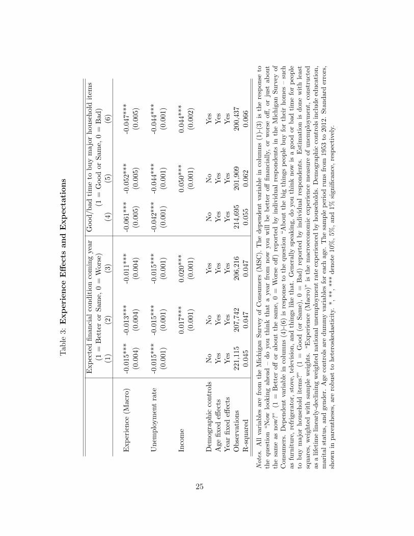
Table 3 shows the corresponding linear least-squares estimations. In columns

(1) to (3), we present the estimates of the relation between prior unemployment-

rate experiences and respondents’ forecasts of their own future situation. We find

that people who have experienced times of greater unemployment during their lives

so far are significantly more pessimistic about their future financial situation. The

statistical and economic significance of the estimated e↵ect is robust to variations

in the controls: Whether we include only (age and time) fixed e↵ects, control for

income, or for all demographic variables, we always estimate a highly significant

coe�cient between �0.015 and �0.011. The robustness of the estimates to the

income control is reassuring since the controls for respondents’ financial situation

are more limited in the MSC data. This renders the estimates in columns (1) to

(3) open to alternative interpretations, especially unobserved wealth e↵ects. When

we include income in columns (2) and (3), the estimation has the expected positive

coe�cient, and the same holds for demographics that might proxy for unobserved

wealth (e. g., education) in column (3). The coe�cient of past experiences of national

unemployment rates remains highly significant and negative.

In terms of the economic magnitude, consider the inter-decile range of lifetime

experiences: Respondents at the 90th percentile are around 2 percentage points more

likely to say financial conditions will be worse in the next 12 months than respondents

at the 10th percentile.

The estimations based on the second question, shown in columns (4) to (6),

generate very similar results. We estimate a significantly negative e↵ect of lifetime

experiences of unemployment on “buying attitude.” The coe�cient is again fairly

stable across specifications, ranging from �0.061 to �0.047. Respondents who have

experienced unemployment rates at the 90th percentile of the sample are around

24

Tab

le3:

Experience

E↵ec

tsand

Expec

tations

Exp

ectedfinan

cial

conditioncomingyear

Goo

d/b

adtimeto

buymajorhou

seholditem

s(1

=Betteror

Sam

e,0=

Worse)

(1=

Goo

dor

Sam

e,0=

Bad

)(1)

(2)

(3)

(4)

(5)

(6)

Exp

erience

(Macro)

-0.015

***

-0.013

***

-0.011

***

-0.061

***

-0.052

***

-0.047

***

(0.004

)(0.004

)(0.004

)(0.005

)(0.005

)(0.005

)

Unem

ploym

entrate

-0.015

***

-0.015

***

-0.015

***

-0.042

***

-0.044

***

-0.044

***

(0.001

)(0.001

)(0.001

)(0.001

)(0.001

)(0.001

)

Income

0.01

7***

0.02

0***

0.05

0***

0.04

4***

(0.001

)(0.001

)(0.001

)(0.002

)

Dem

ographic

controls

No

No

Yes

No

No

Yes

Age

fixede↵

ects

Yes

Yes

Yes

Yes

Yes

Yes

Yearfixede↵

ects

Yes

Yes

Yes

Yes

Yes

Yes

Observations

221,11

520

7,74

220

6,21

621

4,69

520

1,90

920

0,43

7R-squ

ared

0.04

50.04

70.04

70.05

50.06

20.06

6

Notes.Allvariab

lesarefrom

theMichigan

Survey

ofCon

sumers(M

SC).

Thedep

endentvariab

lein

columns(1)-(3)is

therespon

seto

thequ

estion

“Now

look

ingah

ead–doyouthinkthat

ayear

from

now

youwillbebettero↵

finan

cially,or

worse

o↵,or

just

abou

tthesameas

now

?”(1

=Bettero↵

orab

outthesame,

0=

Worse

o↵)reportedby

individual

respon

dents

intheMichigan

Survey

ofCon

sumers.

Dep

endentvariab

lein

columns(4)-(6)is

respon

seto

thequ

estion

“Abou

tthebig

things

people

buyfortheirhom

es–such

asfurniture,refrigerator,stove,

television

,an

dthings

like

that.Generally

speaking,

doyouthinknow

isago

odor

bad

timeforpeople

tobuymajorhou

seholditem

s?”

(1=

Goo

d(orSam

e),0=

Bad

)reportedby

individual

respon

dents.Estim

ationis

don

ewithleast

squares,weigh

tedwithsample

weigh

ts.“E

xperience

(Macro)”

isthemacroecon

omic

experience

measure

ofunem

ploym

ent,

constructed

asalifetimelinearly-decliningweigh

tednational

unem

ploym

entrate

experiencedby

hou

seholds.

Dem

ographic

controlsincludeeducation

,marital

status,an

dgender.Age

controlsaredummyvariab

lesforeach

age.

Thesample

periodrunsfrom

1953

to2012.Standarderrors,

show

nin

parentheses,arerobust

toheteroskedasticity.*,

**,***denote10%,5%

,an

d1%

sign

ificance,respectively.

25

7 percentage points more likely to say now is a bad time to buy major household

items than those at the 10th percentile. This second analysis also addresses con-

cerns unobserved wealth and other unobserved financial constraints even further,

beyond the stability across specifications. Here, respondents are asked about “times

in general,” and the confounds should not a↵ect their assessment of general economic

conditions. Yet, they strongly rely on their personal experiences to draw conclusions

about economic conditions more broadly.

Our results suggest that the economic conditions individuals have experienced in

the past have a lingering e↵ect on their beliefs about the future. Individuals who

have lived through worse times consider their own financial future to be less rosy

and times to be generally bad for spending on durables, controlling for all historical

data, current unemployment, and other macro conditions. This evidence on the

beliefs channel is consistent with prior literature on experience e↵ects, including

Malmendier and Nagel (2011, 2015).

III.C Past Experiences and Future Income

Next we ask whether the long-term reduction in consumption after past unemploy-

ment experiences, as well as the ensuing consumer pessimism, might be the response

to lower employment and earnings prospects. Might the consumer pessimism be

explained by (unobserved) determinants of households’ future income that are cor-

related with past unemployment experiences? As we will show, the answer is no.

To test whether past unemployment experiences are correlated with (unobserved)

determinants of households’ future income, we re-estimate our baseline model from

equation (3) with the dependent variable changed to future income either one or two

or three survey waves in the future, i. e., two, four, and six years ahead.

The estimation results are in Table 4. They suggest that unemployment experi-

ences do not play a significant role in explaining future income. After controlling for

income, wealth, employment status, the other demographics, and fixed e↵ects,18 the

estimated coe�cients of personal unemployment experiences are all positive, small,

and insignificant. For macroeconomic experiences, we estimate small negative coef-

ficients, which are also insignificant with the exception of the estimation predicting

18 All results are similar if we do not include time fixed e↵ects in the regressions, which maymore realistically capture how people form belief given information friction.

26

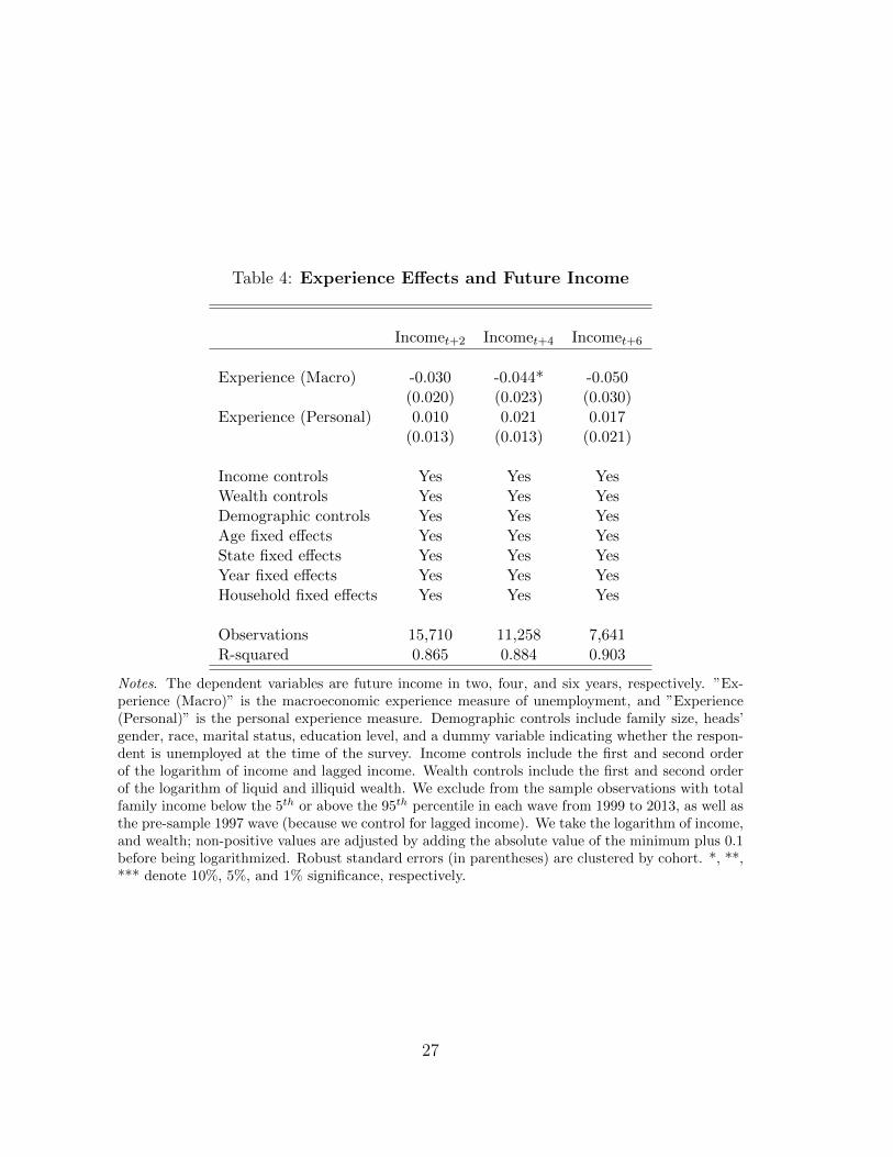
Table 4: Experience E↵ects and Future Income

Incomet+2 Incomet+4 Incomet+6

Experience (Macro) -0.030 -0.044* -0.050(0.020) (0.023) (0.030)

Experience (Personal) 0.010 0.021 0.017(0.013) (0.013) (0.021)

Income controls Yes Yes YesWealth controls Yes Yes YesDemographic controls Yes Yes YesAge fixed e↵ects Yes Yes YesState fixed e↵ects Yes Yes YesYear fixed e↵ects Yes Yes YesHousehold fixed e↵ects Yes Yes Yes

Observations 15,710 11,258 7,641R-squared 0.865 0.884 0.903

Notes. The dependent variables are future income in two, four, and six years, respectively. ”Ex-perience (Macro)” is the macroeconomic experience measure of unemployment, and ”Experience(Personal)” is the personal experience measure. Demographic controls include family size, heads’gender, race, marital status, education level, and a dummy variable indicating whether the respon-dent is unemployed at the time of the survey. Income controls include the first and second orderof the logarithm of income and lagged income. Wealth controls include the first and second orderof the logarithm of liquid and illiquid wealth. We exclude from the sample observations with totalfamily income below the 5th or above the 95th percentile in each wave from 1999 to 2013, as well asthe pre-sample 1997 wave (because we control for lagged income). We take the logarithm of income,and wealth; non-positive values are adjusted by adding the absolute value of the minimum plus 0.1before being logarithmized. Robust standard errors (in parentheses) are clustered by cohort. *, **,*** denote 10%, 5%, and 1% significance, respectively.

27

income four years ahead, where it is marginally significant. In summary, our results

imply that past experiences do not predict future earnings prospects.

Relatedly, one may ask whether past unemployment experiences a↵ect the volatil-

ity of future income. Even if expected income is una↵ected by past experiences, a

consumer might (correctly) perceive the variance of income to be a↵ected. If con-

sumers feel greater uncertainty about the stability of their future employment, they

will save more to mitigate risk and thus consume less as a result. To test if such

a relationship between unemployment experience and income volatility exists, we

re-estimate our baseline model (3) using income volatility as the dependent variable.

Following Meghir and Pistaferri (2004) and Jensen and Shore (2015), we construct

volatiltiy measures both for the transitory and the permanent income. The transi-

tory income-variance measure is the squared two-year change in excess log income,

where excess log income is defined as the residual from an OLS regression of log in-

come on our full slate of control variables. The permanent-income variance measure

is the product of two-year and six-year changes in excess log income (from year t� 2

to t and t � 4 to t + 2, respectively). Appendix-Table A.12 shows the results for

either measure, two, four or six years ahead (i.e., t + 2, t + 4, or t + 6). We do not

find a strong correlation between unemployment experiences and income volatility,

other than one marginally significant coe�cient on macroeconomic experience for

the variance of permanent income in t+2. Hence, consumers’ long-term reduction in

consumption after past unemployment experiences does not appear to be a rational

response to future income uncertainty.

III.D Past Experience and Wealth Build-up

The significant e↵ect of past unemployment experiences on consumption, and the

lack of a relation with future income, imply that household experiences could even

a↵ect the build-up of wealth. In the case of negative lifetime experiences, consumers

appear to restrain from consumption expenditures more than rationally “required”

by their income and wealth positions. This experience-induced frugality, in turn,

predicts more future wealth. Vice versa, consumers who have lived through mostly

good times are predicted to be spenders and should thus end up with less wealth.

In order to test whether experience e↵ects are detectable in long-run wealth

28

accumulation, we relate households’ lifetime experiences to their future wealth, using

up to seven survey waves (14 years) in the future. We consider both liquid wealth

and total wealth. This analysis also ameliorates potential concerns about the quality

of the consumption data and alternative life-cycle interpretations of our findings.

Figure 4 summarizes the coe�cients of interest graphically for 10 regressions,

namely, the cases of wealth at t + 6, t + 8, t + 10, t + 12, and t + 14. The upper

part shows the coe�cient estimates when studying the impact on liquid wealth, and

the lower part shows the estimates for total wealth. All coe�cient estimates are

positive. The impact of macro experiences is smaller and (marginally) significant

only in a few cases, namely, for total wealth in the more recent years and for liquid

wealth further in the future. The estimates of the role of personal lifetime experiences

are much larger and typically significant, with coe�cients ranging from 0.02 to 0.03

for liquid wealth and from 0.08 to 0.10 for total wealth. The estimates imply that

a one-standard deviation increase in personal lifetime experiences of unemployment

will lead to additional precautionary savings and resulting wealth build-up of about

1.3% or $4,500 ten years later. In other word, households who have experienced high

unemployment tend to accumulate more wealth down the road. Appendix-Table

A.13 provides the details on the coe�cient estimates of both experience measures.

In summary, individuals’ lifetime experiences strongly predict consumption ex-

penditure, and beliefs about future economic conditions appear to play a role in

explaining this result. However, such beliefs do not seem to be consistent with ac-

tual income and wealth changes. In fact, we see evidence of a positive relationship

between past experience and future wealth build-up.

IV Consumption with Experience-based Learning

Our four baseline results suggest that past experiences can “scar” consumers. The

combination of expenditure, belief, and future-wealth results are hard to fully ex-

plain in the traditional life-cycle consumption model. However, given the lack of

exogenous, experimental variation in lifetime experiences, it is important to further

explore potential confounds arising from unobserved determinants and frictions.

We utilize the Low, Meghir, and Pistaferri (2010) model to account for sev-

eral frictions and possible confounds, and to illustrate that, for a wide range of pa-

29

Figure

4:W

ealth

Build-u

p:Estim

ated

Coe�

cien

tsand

Confiden

ceIn

tervals

forExperience

Mea

sures

Notes.

Theupper

five

grap

hs(red

bars)

present

theestimates

when

were-estim

ateou

rem

pirical

mod

elusingliqu

idwealth

asthe

dep

endentvariab

le.Thelower

five

grap

hs(bluebars)

show

theestimates

when

weuse

totalwealthas

thedep

endentvariab

le.Thefive

grap

hsin

horizon

talorder

show

theestimated

coe�

cients

when

weuse

6-year

lagged,8-year

lagged,10-yearlagged,12-yearlagged

and

14-yearlagged

experience

measuresrespectively.Alltheconfidence

intervalsareat

90%

confidence

level.

30

rameterizations, we can distinguish experience e↵ects, even directionally. The Low

et al. framework captures a broad array of standard life-cycle consumption factors,

including financial constraints, social-insurance programs, and “income scarring,”

i. e., the notion that job loss reduces income flows because of lower match quality in

future jobs. Moreover, we extend the Low et al. model to include “unemployment

scarring,” i. e., the notion that unemployment, once experienced, makes individuals

inherently less employable. We distinguish both income scarring and unemployment

scarring as well as other life-cycle features from scars due to longlasting experience

e↵ects. The focus of Low et al. is on the interaction of di↵erent types of risk (pro-

ductivity shocks, employment risk) with social insurance (unemployment insurance,

food stamps, and disability insurance). While the social-insurance programs are

not the focus of this paper, they add richness to our analysis and ensure that the

experience-e↵ect estimates are not confounded.

Towards that end, we introduce two classes of consumers into the model: standard

rational agents and experience-based learners. Rational consumers use all available

historical data to update their beliefs about the probability of being unemployed next

period. Experience-based consumers overweight their own experiences when forming

beliefs. We simulate intertemporal consumption and labor decisions for both types of

consumers and estimate the relation between experience measures and consumption

in both settings, i. e., also for rational consumers, for whom they should not have

a significantly negative relation. The simulate-and-estimate exercise illustrates the

basic mechanism of experience-based learning, and distinguishes it from features of

the standard consumption model, such as wealth or liquidity constraints. It provides

guidance towards empirical robustness checks and additional tests.

Low, Meghir, and Pistaferri (2010) Model Setup. Consumers can work for

40 years, until age 62 (starting at age 23), then have mandatory 10 years of retirement

where they receive social-security benefits, and die at the end of retirement. Periods

are quarters, amounting to L = 200 periods of consumption and labor decisions in

total. Their utility function is

U(c, P ) =

�c⇥ e⌘P

�1��

1� �, (4)

31

where c is consumption, and P an indicator equal to 1 if a person works. In each

t, consumer i chooses consumption ci,t and, when applicable, labor supply Pi,t to

maximize lifetime expected utility

maxci,tPi,t

Vi,t = U(ci,t, Pi,t) + Et

"LX

s=t+1

�s�tU(ci,s, Pi,s)

#. (5)

We impose ci,t < At, which rules out borrowing. As we will see below, by max-

imizing the financial constraints of consumers, we are able to derive the sharpest

distinction between the role of experience e↵ects and financial constraints.19 We

assume that flow utility takes a near CRRA form which induces a precautionary

savings motive. (A detailed description of the intertemporal budget constraint and

the social-insurance programs is in Appendix B.)

Income Process The wage in this model is determined by the following formula

lnwi,t = dt + x0i,t + ui,t + ai,j,t0 , (6)

where dt is the log-price of human capital at time t, x0i,t the component determined

by i’s age at time t, ui,t the stochastic component, and ai,,j,t0 the job-fit component

of i’s wage at firm j for a job o↵ered (and accepted) in period t0. Gross quarterly

income is wi,th, where h is the number of hours worked in a quarter. The three social-

insurance programs Low et al. include in their model are detailed in Appendix B.

Agents have the ability to make decisions about whether or not to work. For

example, agents need not work if an o↵er is too low. They can also retire early. Note

that this implies that experienced-based learners may make di↵erent labor supply

choices depending on their concern about future employment and desire to save.

The Deterministic Component of Wage. The deterministic component of

wage dt + x0it is the same for all individuals of a given age at time t. The size of

19 The reason is that (unobserved) financial constraints are a potential confound of the empiricalrelation between prior experiences and consumption: Younger cohort tend to be more constrainedin their borrowing ability and are predicted to react more strongly to a shock than older cohortsunder the experience-e↵ect hypothesis. By eliminating borrowing altogether from the simulation,we maximize the impact of financial constraints.

32

this component is estimated via regression in Low et al. and of the form20

dt + x0i,t = ↵ + �1 · age + �2 · age2. (7)

The Permanent Component of Wage. The stochastic component of the wage

ui,t is determined by a random walk. Consumers receive a shock to this component

on average once a year. If consumer i has an income shock in period t, then ui,t is

ui,t = ui,t�1 + ⇣i,t, (8)

where ⇣i,t is i. i. d. normal with mean 0 and variance �2⇣ .

The Job-Match Component of Wage. A key element of the Low et al. model

is its job-match process. The consumer-firm job-match component, ai,j,t0 , is drawn

from a normal distribution with mean 0 and variance �2a. It is indexed by the period

t0 in which the consumer joined firm j, and not by t, since it is constant throughout

the duration of the consumer-firm interaction.

Job Arrival. In each period, the probability of job destruction is �, the proba-

bility of a job o↵er is (1 � �)�e for an employed worker, and �n for an unemployed

worker. Agents receive job o↵ers with varying job matches. By construction, they

accept all o↵ers with a higher job match and reject all o↵ers with a lower job match.

The job match component, in combination with the processes of job destruction

and job generation, is at the core of the “income scarring” result of Low et al.

(2010). While employed, people successively trade up for jobs that are a better

match. They thus gain higher incomes over their life-cycle. In turn, if they experience

job destruction, they lose their job match and must (re-)start getting better and

better job o↵ers. Hence, agents typically earn a lower income after an unemployment

spell, and job loss leads to a long-lasting reduction in earnings. By accounting for

rational “income scarring,” we impose a high bar on our hypothesis. We test whether

experienced-based learners reduce their consumption beyond this bar.

Belief Formation. Both types of consumers, rational and experience-based learn-

ers, know the model, but di↵er in their beliefs about the probability of job loss �.

20 While x0i,t includes a larger set of control variables in the empirical portion of Low et al., only

age and age squared are used to fit a general lifetime income profile to the model.

33

We denote consumer i’s believed probability of job destruction at time t as �bi,t. Ra-

tional consumers use all available data on unemployment to update their beliefs. If

they have lived long enough, they know (or closely approximate) the true value of

�, �bi,t = � 8t. Experience-based learners form their belief based on the history of

realizations in their prior lives. Applying specification (1), with weighting scheme

(2), we obtain

�bi,t =t�1X

k=1

w (�, t, k)Pi,tDi,t�k, (9)

where Di,t is an indicator of i experiencing job destruction in t, and

w(�, t, k) =(t� k)�

Pt�1k=0 Pi,t (t� k)�

. (10)

is the weight assigned to realizations D at k periods before period t.

Model Estimates on Experience E↵ects in Consumption. We simulate the

consumption-saving decisions for both rational and behavioral consumers using the

parameters in Table 5.21 The values are identical to those in Low et al. (2010)

whenever possible. Following Low et al., we distinguish between high- and low-

education individuals by varying the corresponding parameters.

We show several plots of the resulting consumption paths for both rational and

experience-based learners in Appendix B. In particular, we separate consumers who

were “lucky” and “unlucky” early in life, in terms of their earnings in Figures B.2

and B.3. The graphs illustrate the corresponding over- and underconsumption of

experience-based learners during their early lifetime, relative to rational consumers,

as well as the need to then curtail consumption later in the first case (good expe-

riences) and the excess wealth build-up in the second case (bad experiences). This

corresponds to the empirical relationship we found in Section III.D.

Using the simulated values, we estimate the relationship between consumers’

unemployment experience and consumption behavior, controlling for income and

wealth. The corresponding OLS regressions are in Table 6, columns (1) and (2),

for rational consumers, and in columns (3) and (4) for experience-based learners.

In the case of rational agents, prior experiences do not actually enter their belief

21 The full list of parameters is in Appendix-Table B.1.

34

Table 5: Key Simulation Parameters

Parameter Benchmark value(s)Preference parameters

Relative risk aversion coe�cient ⇢ 1.5Interest rate r 1.5%Discount factor � 1/(1 + r)

Lifetime parametersWorking years 40Retirement years 10

Income process High education Low educationStandard deviation of job matches �a 0.226 0.229Standard deviation of permanent shocks �⇣ 0.095 0.106

formation. The purpose of including the experience measure here is to identify

possible confounds of the significantly negative e↵ect we have estimated in the PSID

data. Specifically, as we are concerned about unobserved wealth e↵ects, we estimate

one model where we do not include wealth as a control (column 1) and one where we

include wealth (column 2), in both cases in addition to the experience-e↵ect proxy.

Income scarring. We first conduct the simulation using linearly declining

weights (� = 1) for the measure of prior experiences, as we did in our empirical

analysis. As shown in the top panel of Table 6, income has the expected positive

sign and significance across specifications, as does wealth when it is included. More

noteworthy is that, when using the simulations with rational agents (columns 1 and

2), we estimate a positive coe�cient of the experience measure, indicating that higher

unemployment experiences predict higher consumption. This is the opposite of what

we find empirically, and a first step towards ameliorating concerns about confounds:

It appears to be hard to (falsely) estimate a negative experience e↵ect when agents

are rational, whether or not we include perfect wealth controls.

When we alter the belief-formation process to experience-based learning, instead,

we estimate a significant negative coe�cient, both without and with wealth control

(columns 3 and 4). That is, lifetime experiences strongly predict consumption behav-

ior of experience-based learners, after taking into account their income and wealth.

Compared to the results obtained empirically, the coe�cients on unemployment ex-

perience in columns 3 and 4 are greater in magnitude, which may be attributed to

the lack to other control variables in the simulation exercises.

35

Table 6: Estimations with Model-Simulated Data

(1) (2) (3) (4)Rational Rational EBL EBL

� = 1:Income 0.576 0.383 0.606 0.398

(244.87) (67.63) (197.97) (55.72)Wealth 0.261 0.264

(52.30) (57.34)Unemployment Experience 0.0975 0.398 -0.392 -0.762

(2.08) (3.24) (-9.01) (-9.49)� = 3:Income 0.567 0.379 0.619 0.401

(137.52) (50.58) (163.45) (52.05)Wealth 0.265 0.270

(40.46) (63.31)Unemployment Experience 0.280 0.286 -0.200 -0.576

(4.85) (3.39) (-7.48) (-9.97)� = 0:Income 0.569 0.382 0.598 0.397

(209.47) (236.72) (198.14) (55.39)Wealth 0.260 0.259

(52.52) (50.97)Unemployment Experience -0.135 0.397 -0.496 -1.027

(-3.18) (3.20) (-8.37) (-8.39)

Notes. Estimations with simulated consumption values as the dependent variable and simulatedsame-period income and wealth as regressors, for rational consumers in columns (1) and (2), andexperienced-based learning (EBL) consumers in columns (3) and (4). Estimations are for with� = 1 in the top panel, � = 3 in the middle panel, and � = 0 in the bottom panel. Consumption,income, and wealth are in log terms. All estimations include period and education fixed e↵ectsand use period-clustered standard errors. Simulations are based on the working periods of 10,000simulated consumers and thus 1,600,000 observations. t statistics in parentheses.

36

The results are qualitatively and quantitatively similar when we put higher weights

on consumers’ recent experiences (� = 3), as shown in the middle panel of Table 6.

Note that the positive sign of the experience-e↵ect estimate in the data simulated

for rational agents (columns 1 and 2) not only ameliorates concerns about wealth

confounds, but also seems to contradict the basic intuition of “income scarring:”

Unexpected job destruction lowers lifetime income, and thus consumption. Why

do higher unemployment experiences predict higher consumption? To understand

this result, consider two consumers, A and B, with the same income. A has experi-

enced unexpected job loss in the past, while B has not. All else held equal, “income

scarring” predicts that A earns less. However, by assumption, A and B have the

same income, suggesting that A’s wage is driven by her permanent-income compo-

nent rather than her job-match component. As a result, A is less worried about

unexpected job destruction and rationally consumes more. In other words, if one

introduces a proxy for experience e↵ects into a world with rational agents, it can

act as a proxy for the permanent-income component and generate the opposite sign.

Under this scenario, there is little concern about confounding experience e↵ects with

traditional determinants of lower consumption, including (unobserved) wealth e↵ects

and income scarring, as long as we control for current income.

To recover the intuition of income scarring and generate a negative relationship

between the experience measure and consumption under rational learning, we can

employ an experience measure that is more backward looking. In our model, this

amounts to lowering �. In the bottom panel of Table 6, we repeat the estimation set-

ting � = 0, so all prior experiences get equal weights. In this case, the specification

with rational learners and without wealth control (in column 1) shows a negative

correlation between unemployment experience and consumption. That is, for � = 0,

we see “income scarring” and its possible confound at work: If two people have the

same income today, but one person got fired more in the past, then that person likely

has earned less in the past, thus has lower assets today, and consumes less. However,

once we control for asset accumulation (in column 2), we re-estimate a positive co-

e�cient on unemployment experiences, with all coe�cients being similar to the ones

estimated for � = 1 (column 2 of the upper panel). At the same time, the estimated

experience e↵ect is robustly negative for experience-based learners, both with and

without wealth control, as shown in columns (3)-(4) of the lower panel. In other

37

words, under a more backward-looking proxy for experience e↵ects the potential

wealth confound materializes: If we do not control for wealth, the experience-e↵ect

proxy might pick up those e↵ects even though agents are not experience-based learn-

ers. If agents are experience-based learners, we expect to robustly identify their

experience-induced consumption adjustment.

Table 7: Estimations with Model-Simulated Data, Unemployment Scarring

(1) (2) (3) (4)� = 1 � = 1 � = 3 � = 3

Rational EBL Rational EBLIncome 0.282 0.350 0.284 0.371

(141.89) (65.34) (123.91) (59.28)Wealth 0.314 0.260 0.311 0.262

(54.31) (32.30) (55.01) (35.44)Unemployment Experience 0.176 -1.757 0.138 -1.493

(2.88) (-25.31) (3.06) (-31.06)

Notes. Estimations with simulated consumption values as the dependent variable and the simulatedsame-period income and wealth as regressors for rational consumers. The simulations account forunemployment scarring. Consumption, income, and wealth are in log terms. The experience proxyis calculated with � = 1 in columns (1) and (2) and � = 3 in columns (3) and (4). All estimationsinclude period and education fixed e↵ects and use period-clustered standard errors. Simulationsare based on the working periods of 10,000 simulated consumers and thus 1,600,000 observations.t statistics in parentheses.

Unemployment scarring. As a last step, we consider an even higher hurdle to

the identification of experience e↵ects, and introduce additional negative correlation

between unemployment and future income as an alternative explanation. Our moti-

vation for introducing such “unemployment scarring” comes from research in labor

economics that has found a persistent negative e↵ect of being unemployed on future

income, especially during a recession (Davis and Von Wachter 2011, Huckfeldt 2016,

Jarosch 2015). While those findings might actually be evidence for experience e↵ects,

the existing literature proposes more traditional explanations. The model of “unem-

ployment scars” in Jarosch (2015), for example, features a job-security component

that resembles the “job-match component” of wages in Low, Meghir, and Pistaferri

(2010), albeit with the di↵erence is that wage gains lost due to “income scarring”

can be regained by working for an extended period.22

22 See the ✓y component of the firm-type vector in Section 2.1 of Jarosch (2015).

38

To add “unemployment scarring” to our simulation, we reduce a consumer’s per-

manent wage component by the average size of a permanent income shock, �⇣ , every

time she experiences job destruction. We re-simulate the model with this additional,

permanent e↵ect of job loss on income, and then re-estimate the specifications of

Tables 6, i. e., analyze again which e↵ects the experience proxy might pick up in

estimations using simulated data with rational agents, and whether it identifies ex-

perience e↵ects in estimations using simulated data with experience-based learners.

Table 7 shows the results for rational and for EBL agents, both for � = 1 and

for � = 3, in the specifications controlling for wealth. We find that the signs and

significant levels of all coe�cients remain the same as in the simulation without

unemployment scarring. For the simulations with rational agents, the coe�cient on

the experience-e↵ect proxy remains significantly positive both for � = 1 and for � =

3,23 though the size of the coe�cients becomes (mechanically) lower. Intuitively, the

experience measure still acts as an indirect proxy for a high permanent component,

but now for a subgroup where the permanent component has been systematically

reduced compared to the baseline model: Observing two people A and B with the

same income today, where only A has experienced unemployment, still suggests that

A has a higher permanent component. However, A’s distribution of the permanent

component will be shifted down by one standard deviation (unemployment scarring).

Overall, these results provide evidence that our predictions are robust even when

future income and unemployment are strongly negatively correlated due to both “in-

come scarring” and “unemployment scarring.” For empirically validated parameter-

izations of experience e↵ects (with linearly declining or steeper weighting functions),

financial constraints, unobserved wealth factors, income scarring, and unemployment

scarring fail to generate a negative relation between our proxy for past unemployment

experiences and consumption when agents are Bayesian learners. Instead, a negative

coe�cient estimate likely indicates experience-based learning. The same holds when

varying the unemployment-experience proxy further to overweight past experiences

even more (e. g., equal weighting all life-time experiences) as long as we control for

wealth e↵ects. However, if we fail to appropriately control for wealth e↵ects under

those latter flat weighting functions, the confound might materialize. We do not im-

23 As before, we estimate a positive coe�cient even when not controlling for wealth, unless wealter the experience proxy to further overweight experiences far in the past, i. e., for very low �’s.

39

plement the latter specifications empirically; nevertheless, the simulate-and-estimate

exercise with those parameters indicates that it is important to conduct exhaus-

tive robustness checks with a variety of alternative wealth specifications—including

varying proxies for liquid versus illiquid wealth, higher-order terms, decile dummies,

separate dummies for housing wealth or for positive wealth versus debt, and for com-

pleteness a similar battery of variations of the income controls. We will also use the

model to generate additional predictions of the experience-e↵ect model that are not

generated by alternative interpretations.24

V Robustness using PSID, CEX, and Nielsen

Guided by the theoretical model, we re-estimate the consumption model with a

battery of alternative and additional wealth, income, and liquidity controls using the

PSID data. We then turn to the CEX and the Nielsen data, both for replication

and, in Section VI, to examine additional predictions of the experience-e↵ect model.

V.A PSID: Wealth, Income, and Liquidity

We start from concerns about imperfect measurement of individual wealth. Our

simulate-and-estimate exercise in Section IV alleviates these concerns, as it appears

hard to generate misattribution under our standard proxy for experience e↵ects and

given the controls for unemployment status and income – even in the presence of

such mismeasurement. Moreover, our prior results on future wealth build up, future

income, and beliefs are also hard to reconcile with the unobserved-wealth interpreta-

tion. Nevertheless, we use a battery of alternative wealth measures, which we include

in addition to the first- and second-order liquid- and illiquid-wealth controls that are

already included in Table 2: (1) third and fourth order controls of (log) illiquid and

illiquid wealth, (2) wealth decile dummies, separately for liquid and illiquid wealth,

(3) log home equity value (home price minus mortgage) and log non-housing wealth,

24 One prediction we did not pursue regards the hours worked. In general, EBL implies apositive relation between past unemployment experience and the likelihood of working because workgenerates greater income bu↵er. (Note that “work” is a binary decision in the model.) However,this prediction does not hold if income or unemployment scarring is strong. In that case, the costof working dominates the gain, and consumers are more likely to choose living o↵ social welfareprograms instead of working.

40

and (4) log total debt and log positive wealth separately. We summarize all esti-

mated coe�cients of the macro and personal experience measures in the left panel

of Figure 5. (The detailed results are in Appendix-Table A.9.) All coe�cients of

interest remain very similar, both in size and in statistical significance.

A related concern is measurement error in the income variable. As with wealth,

we re-estimate our empirical model using varying constructs of income: (1) third and

fourth order of (log) income and lagged income, (2) quintile dummies of income and

lagged income, (3) decile dummies of income and lagged income, and (4) controls

the bottom 2, 2nd-4th, 4th-6th, 6th-8th, 8th-10th, 90th-92nd, 92nd-94th, 94th-96th, 96th-

98th, and top 2 percentile dummies of income and lagged income. The estimated

coe�cients of interest, shown in the right panel of Figure 5, are again similar in both

magnitude and significance. All estimates are in Appendix-Table A.10.

A more specific concern is related to the role of liquidity. Even though the results

are robust to variations in wealth measures, might the estimated experience e↵ect

still be confounded with (unmeasured) liquidity constraints? Our separate controls

for liquid and illiquid wealth in the baseline estimations in Table 2 and in columns

(2) and (6) of Appendix-Table A.9, ameliorate these concerns. As a further step, we

test whether the consumption of households that are disproportionately likely to be

liquidity constrained, as proxied by their low liquid-assets position, are more a↵ected

by their unemployment experience. Closely following the practice in the consump-

tion literature, such as Johnson, Parker, and Souleles (2006) and Parker, Souleles,

Johnson, and McClelland (2013), for each year we sort households into two groups

based on whether their liquid wealth lies above or below the median liquid-wealth

level in the sample. Expanding equation (3), we interact an indicator for being in

the below-median group and the experience variables. As shown in Appendix-Table

A.11, households in the bottom half of the liquid-wealth group tend to spend less

relative to households in the top half on average. However, their consumption expen-

diture does not exhibit a significantly stronger reaction to unemployment experience.

All coe�cients are either insignificant or point in the opposite direction. This sug-

gests that the negative e↵ect of unemployment experiences on consumption is not

explained by liquidity constraints.

41

Figure

5:W

ealthandIn

comeControls:Coe�

cien

tsandConfiden

ceIn

tervals

forExperience

Mea

sures

Dep

ende

nt V

aria

ble:

Foo

d C

onsu

mpt

ion

Dep

ende

nt V

aria

ble:

Tot

al C

onsu

mpt

ion

Dep

ende

nt V

aria

ble:

Foo

d C

onsu

mpt

ion

Dep

ende

nt V

aria

ble:

Tot

al C

onsu

mpt

ion

A. W

ealth

B. I

ncom

e

Mea

sure

1M

easu

re 2

Mea

sure

3M

easu

re4

Mea

sure

5M

easu

re6

Mea

sure

7M

easu

re8

Notes.Thered(dark)

barsin

theupper

leftqu

adrant

present

theestimates

when

weuse

food

consumption

asthedep

endentvariab

lean

dincludefouralternativewealthcontrols:(1)third-an

dfourth-order

liqu

idan

dilliqu

idwealth,(2)deciledummiesforliqu

idwealthan

dilliqu

idwealth,(3)hou

singwealthan

dother

wealth(total

wealthminushou

singwealth),

and(4)positivewealthan

ddebt.

Allwealth

controls

arein

additionto

first-

andsecond-order

liqu

idan

dilliqu

idwealth.Theblue(light)barsin

thelower

left

quad

rant

show

the

estimates

when

weuse

totalconsumption

asthedep

endentvariab

lean

dthesamefoursets

ofwealthcontrols.Thered(dark)

barsin

theupper

righ

tqu

adrant

present

theestimates

when

weuse

food

consumption

asthedep

endentvariab

lean

dincludefouralternative

incomecontrols:(1)third-an

dfourth-order

incomean

dlagged

income,

(2)qu

intile

dummiesforincomean

dlagged

income,

(3)decile

dummiesforincomean

dlagged

income,

and(4)separatedummiesforthebottom

2,2n

d�4t

h,4t

h�6t

h,6t

h�8t

h,8t

h�10

th,90

th�92

nd,

92nd�

94th,94

th�

96th,96

th�

98th,an

dtop2percentiles

ofincomean

dlagged

income.

Allincomecontrols

arein

additionto

first-

andsecond-order

incomean

dlagged

income.

Theblue(light)barsin

thelower

righ

tqu

adrant

show

theestimates

when

weuse

total

consumption

asthedep

endentvariab

lean

dthefourincomecontrols.Allregression

sincludehou

seholdfixede↵

ects.Con

fidence

intervals

areat

the90%

confidence

level.

42

V.B CEX

Next, we turn to a second source of consumption data, the Consumer Expenditure

Survey (CEX). We now enlarge the set of consumption items to include durable

goods as well as the CEX measure of total consumption, which is widely used in the

literature. It encompasses further categories of expenditures, in addition to durables

and non-durable items, including healthcare and education expenses.25

The CEX is a repeated cross-sectional survey of household spending across a

comprehensive list of product categories at the quarterly frequency. It is considered

the benchmark data in the consumption literature. Compared to the PSID, its two

main disadvantages are the lack of wealth information and the lack of panel structure.

As in the analysis of the PSID, we link measures of consumption to households’

lifetime unemployment experiences. As before, we construct lifetime experiences as

the weighted average of experienced unemployment outcomes since birth, using lin-

early declining weights. In the CEX data, we are not able to construct the same type

of macro and personal unemployment experience measures as in the PSID because

the CEX does not provide information on where households resided prior to the sam-

ple period, nor on their prior employment status. We use the macro-level experience

measure based on national unemployment rates at the quarterly frequency.

The top panel of Table 8 provides the summary statistics. The average income,

$47k, is in line with the average income at the national level. The sample period

runs from 1980-2012. Note that durable and non-durable consumption do not add

up to total consumption because of expenditures that are not considered durable or

non-durable, such as healthcare and education expenses. The average non-durable

and durable spending amount to 67.9% and 20.0% of the mean total expenditures,

respectively. Non-durable spending and durable spending are weakly positively cor-

related, with durable spending being much more volatile than non-durable spending.

We re-estimate the sensitivity of consumption to experienced unemployment con-

ditions, using an estimation model that closely mirrors the PSID model from equation

(3). Table 9 shows the results for total, durable, and non-durable consumption.

25 Estimations involving durable consumption can be a↵ected by the timing of durable purchases.Prior research such as Bar-Ilan and Blinder (1992) and Berger and Vavra (2015) shows that durablepurchases tend to be discontinuous and go down during recessions. However, these concerns do notapply to our estimates of experience e↵ects on food and other non-durable consumption items.

43

Table 8: Summary Statistics (CEX and Nielsen)

Variable Mean SD p10 p50 p90 NCEX (Quarterly)Age of male head of HH 51 17 29 49 75 417,607Income 47,220 48,925 8,634 33,728 100,000 417,607Household size 2.7 1.5 1 2 5 417,607Total expenditure 6,116 6,145 1,902 4,490 11,479 417,607Non-durable expenditure 4,152 3,189 1,537 3,452 7,364 417,607Durable expenditure 1,226 4,082 0 170 2,085 417,607Experience (Macro) 6.1 0.3 5.8 6.0 6.5 417,607

Nielsen (Monthly)Age of male head of HH 50 12 33 49 67 3,171,833Income $50-$60k $20-$25k $50-$60k $100k+ 3,171,833Household size 2.8 1.5 1 2 5 3,171,833Total expenditure 714 537 205 586 1,366 3,171,833Coupon use 0.03 0.05 0 0.01 0.09 3,171,833Product ranking 0.47 0.11 0.34 0.47 0.61 3,171,833Purchase of sale items 0.24 0.24 0 0.17 0.62 3,171,833Experience (Macro) 6.0 0.2 5.8 5.9 6.3 3,171,833

Notes. The top panel shows quarterly CEX data from 1980-2012. The bottom panel shows monthlyNielsen data from 2004-2013. Nielsen reports income in 13 brackets. Coupon use is the value ofcoupons divided by total expenditures. Product ranking ranges from 0 to 1 based on the unit priceof a good within its product module and market in a given month; lower-priced goods have lowervalues. Purchase of sale items is the number of sale items divided by the total number of itemsbought. Experience (Macro) is households’ lifetime experience of national unemployment rates.

The results strongly confirm our prior findings, and reveal new quantitative im-

plications for the di↵erent components of total consumption. All experience e↵ect

coe�cients are negative and highly significant. Households who have experienced

worse unemployment conditions during their lifetime spend significantly less in to-

tal, durable, and non-durable consumption. The economic magnitudes are large:

A one standard-deviation increase in unemployment experience is associated with

a decline in annual consumption of $432 for non-durables and $564 in total. The

estimate on non-durable consumption is larger than in the PSID ($276 decline in

annual food consumption), while the estimate on total consumption is smaller than

the PSID estimate ($912 decline). This may reflect the fact that non-durable in

the CEX include leisure, which tends to be elastic, while total expenditures in the

CEX encompass healthcare and education, which tend to be more inelastic. The

44

Table 9: Experience E↵ects and Quarterly Consumption (CEX)

Total Durables Non-durable

Experience (Macro) -0.077*** -0.085*** -0.086***(0.010) (0.027) (0.005)

Income control Yes Yes YesHousehold controls Yes Yes YesAge fixed e↵ects Yes Yes YesTime fixed e↵ects Yes Yes YesRegion fixed e↵ects Yes Yes Yes

Observations 417,607 417,607 417,607R-squared 0.390 0.126 0.409

Notes. Pooled regressions with (log) total consumption expenditure, durable consumption, and

non-durable consumption as the dependent variables. “Experience (Macro)” is the macroeconomic

experience measure of unemployment, constructed as a lifetime linearly-declining weighted national

unemployment rate experienced by households. Household characteristics include unemployment

status, household size, education, and race. Time fixed e↵ects include year-quarter fixed e↵ects.

Region fixed e↵ects include dummies for the Northeast, Midwest, South, and West region. Regres-

sions are weighted by household sampling weights from CEX. The sample period runs from 1980

to 2012. Robust standard errors (in parentheses) are clustered by cohort. *, **, *** denote 10%,

5%, and 1% significance, respectively.

new estimate for durables indicates that a one standard-deviation increase in past

unemployment experience predicts a $120 decline in annual durable consumption.

V.C Nielsen

As a final source of data on consumption choices, we turn to the Nielsen Homescan

Dataset. The Nielsen data contains information on product purchases of a panel of

more than 100,000 U.S. households from 54 geographically dispersed markets, each

roughly corresponding to a Metropolitan Statistical Area (MSA), from 2004-2013.

The households provide detailed information about their purchases, including price,

quantity, date of purchase, identifier of the store, as well as product characteristics,

including brand, size and packaging, at the Universal Product Code (UPC) level.

Households record the dollar value of any coupons used and whether the purchase

involved a deal from the retailer (sale item). The product categories are food and

45

non-food grocery, health and beauty aids, and general merchandise, summing to

approximately 3.2 million unique UPCs covering 125 general product categories.26

Households also report information on their demographics, including age, sex,

race, education, occupation, employment status, family composition, household in-

come, and location of residency up to the zip code level. Note that the geographic

information is more precise than the state-level identification in the PSID, as it allows

us to control for the local (county-level) unemployment rate Umt. The information is

updated annually, and the demographics of the households are representative of the

population demographics at the national level. For our analysis, we drop households

with heads below the age of 25 or above 75, as in the PSID sample.27

Our data sample consists of 3,171,833 observations of 105,061 households. The

bottom panel of Table 8 provides the summary statistics. We note that the aver-

age consumption expenditure from Nielsen approximately corresponds to the food

consumption expenditures in the PSID, which cross-validates the quality of the data

sets as the Nielsen data covers mostly food products.

We also conduct a robustness analysis that keeps the advantages of the Nielsen

panel structure but exploits the comprehensiveness of the CEX by creating a syn-

thetic Nielsen-CEX panel. Details and estimations are in Appendix-Section A.2.

The high-frequency nature of the Nielsen data allows us to construct more precise

experience measures than the PSID. However, we are not able to construct the same

type of macro and personal unemployment experience proxies as in the PSID because,

like the CEX, Nielsen provides no information about households’ prior residence or

employment status (pre-sample period). We thus construct the macro-level experi-

ence measure based on national unemployment rates. For the personal experience

measure, we can, at best, measure unemployment experiences since the beginning

of the Nielsen data. Such a measure is necessarily biased, as it is less precise at the

beginning of the sample and for shorter household spells. We therefore report the

estimations employing only the macro-experience measure in the main text.28

26 Several studies have examined the quality of the data. For example, Einav, Leibtag, and Nevo(2010) compare the self-reported Nielsen data with data from cash registers. They conclude thatthe reporting error is of similar magnitude to that found in commonly used economic data sets.

27 As in the PSID data, we also conduct the analysis on a subsample that excludes householdsover the age of 65 (retirees) whose expectation of their future income should be immune to beliefsabout future economic fluctuations. The results from both sets of regressions are similar.

28 We have re-estimated our model using a measure of personal unemployment experience that

46

Like the CEX, Nielsen lacks information about consumers’ wealth, which is an

important component of consumption analyses. Our prior estimations alleviate con-

cerns about unobserved wealth to some extent, given the comparable estimates across

the PSID data (with wealth controls) and the CEX, and given the robustness of the

estimates across a broad range of wealth, income, and liquidity proxies. To further

address the issue of the missing wealth control in the Nielsen data, we follow recent

advancements in the literature, such as Stroebel and Vavra (2017) and Dube, Hitsch,

and Rossi (2018), and use ZIP-code level house prices as a measure of housing wealth.

According to these studies, consumption dynamics respond strongly to house price

movements and housing wealth (see also Mian, Rao, and Sufi (2013) and Berger and

Vavra (2015)). Empirical analyses can exploit this insight since better measures of

housing prices have become available. Specifically, we extract Zillow’s Home Value

Index at the local ZIP code level as a proxy for local housing prices,29 and merge

it with the Nielsen data. The match rate lies around 75%, and the resulting data

set contains almost 3.2 million observations. We include the Home Value Index, an

indicator for being a homeowner, and their interaction in all of our estimations.30

To re-estimate the sensitivity of consumption to experienced unemployment con-

ditions in the Nielsen data, we use an estimation model that again closely mirrors

the PSID model from equation (3), but accounts for the additional market-level

information:

Cit = ↵ + �UEit + Umt + �0xit + ⌘t + &m + �i + "it. (11)

The new variables are the current county-level unemployment rate Umt and local-

market dummies &m, where local markets denote Nielsen’s designated market areas

(DMAs).31 As before UEit denotes the lifetime (macro) experience of unemployment

takes the value 1 at time t if the head of household has ever been unemployed since the beginningof the sample period up to time t� 1, and 0 otherwise. The coe�cient of interest remains similar.

29 Zillow Inc. collects detailed data on home values across the U.S. and constructs monthly indicesusing the median value for a ZIP code. Zillow’s estimates of home values (“Zestimates”) aim toprovide realistic market values given the size, rooms, and other known attributes of the house, recentappraisals, geographic location, and general market conditions. (The exact formula is proprietary.)For details about the data and Zillow’s coverage across the U.S. see Dube, Hitsch, and Rossi (2018).

30 We also conduct the analysis without including these wealth controls in the regressions, andthe coe�cient on unemployment experience remains significant and of very similar magnitude.

31 DMAs are slightly bigger than a county but smaller than an MSA. We control for location at

47

rates. The vector of controls xit includes income controls, wealth controls, household

characteristics (unemployment status, household size, education, race, and a dummy

variable indicating whether the respondent is unemployed at the time of the survey),

and age dummies, and the time dummies ⌘t are now year-month-specific. Standard

errors are clustered at the cohort level. All regression results are quantitatively and

qualitatively similar when clustered by household, household-time, cohort-time, or

two-way clustered at the cohort and time level.

Table 10 present results from regression specification (11). Columns (1)-(2) show

estimates from pooled OLS regressions, and columns (3)-(4) from regressions with

household fixed e↵ects, thus controlling for time-invariant unobserved heterogeneity

at the household level. We find that, exactly as in the PSID data, households who

have experienced worse unemployment conditions during their lifetimes so far spend

significantly less, controlling for contemporaneous macro conditions, local market

conditions, and household controls. The economic magnitude is significant: A one

standard deviation increase in unemployment experiences is associated with a $708

decline in annual consumption of non-durables, which amounts to around 8% of

average spending for the households in our sample. When we introduce household

fixed e↵ects, the estimated experience e↵ects become smaller – as expected given

that we are di↵erencing out the cross-sectional di↵erences in consumption between

households with “mostly good” versus “mostly bad” lifetime experiences. Now, a one

standard deviation increase in unemployment experiences predicts a $300 decline in

annual non-durable consumption, comparable to the PSID estimates.

In Figure 6, we illustrate the economic magnitude of the estimates in the context

of unemployment conditions during the Great Recession, which falls in the Nielsen

sample period. The average monthly unemployment rate from 2008-2012 was 8.1%,

with the maximum during the period being 10%. Comparing these numbers with

historical averages, the average unemployment rate during the 60 years prior to 2008,

from 1947-2007, was 5.6%. Now consider two individuals, a 25-year-old and a 60-

year-old as of December 2007. Their lifetime unemployment experience, based on our

experience weighting scheme, was 5.3% and 5.8%, respectively, when they entered

the crisis in 2008. By the end of 2012, their lifetime unemployment experience was

the local market level instead of the county level because people may travel outside of counties topurchase goods. The results are similar if we use county fixed e↵ects instead.

48

Table 10: Experience E↵ects and Monthly Consumption (Nielsen)

(1) (2) (3) (4)

Experience (Macro) -0.415*** -0.415*** -0.178*** -0.177***(0.044) (0.044) (0.034) (0.034)

Unemployment rate (county) -0.002 -0.005***(0.003) (0.001)

Income control Yes Yes Yes YesWealth control Yes Yes Yes YesHousehold characteristics Yes Yes Yes YesAge fixed e↵ects Yes Yes Yes YesTime fixed e↵ects Yes Yes Yes YesMarket-area fixed e↵ects Yes Yes Yes YesHousehold fixed e↵ects No No Yes Yes

Observations 3,171,833 3,171,833 3,171,833 3,171,833R-squared 0.116 0.116 0.526 0.526

Notes. Pooled OLS and fixed e↵ects regression with (log) total consumption expenditure as the de-pendent variable. Experience (Macro) is the macroeconomic experience measure of unemployment,constructed as a lifetime linearly-declining weighted national unemployment rate experienced byhouseholds. Wealth controls include the ZIP-code level house-price index from Zillow, an indicatorvariable for households that own at least one house, and an interaction term between the houseprice index and the homeowner dummy. Household characteristics include unemployment status,household size, education, race, and a dummy variable indicating whether the respondent is unem-ployed at the time of the survey. Time fixed e↵ects are year-month fixed e↵ects. Regressions areweighted using the household sampling weights from Nielsen. The sample period runs from 2004to 2013. Robust standard errors (in parentheses) are clustered by cohort. *, **, *** denote 10%,5%, and 1% significance, respectively.

49

Figure 6: Example of Unemployment Experience Shock from Recession,Nielsen

5.3%

6.3%5.8% 6.1%

$575.3$477.5

$727.4 $691.0

0

200

400

600

800

1000

0

1

2

3

4

5

6

7

2007 2012Birth year = 1982 Birth year = 1947

Life

tim

eEx

peri

ence

of

Une

mpl

oym

ent

(in %

, bar

s)

Monthly Expenditure (in

$, lines)

-5%

-17%

Notes. Example of the impact of the Great Recession on weighted lifetime experiences of unem-ployment rates and monthly consumption expenditure of a 25- and a 60-year-old (as of 2007) fromDecember 2007 to December 2012. The bars show the weighted lifetime experiences of unemploy-ment rates based on linearly-declining weights. The lines show the monthly expenditures: the valuesfor 2007 are from actual data, and the values for 2012 are calculated based on model estimates.

6.3% vs. 6.1%, respectively. In other words, the unemployment experience for the

25-year-old increased by 1 pp, whereas that for the 60-year-old increased by 0.3pp.

Relating these experiences to consumption behavior, our model estimates imply that

the monthly consumption expenditure of the 25-year-old decreased by approximately

18% while that of the 60-year-old decreased by approximately 5%.

VI Further Implications and Discussion

Building on the robust results on the relation between past unemployment experi-

ences and consumption in the PSID, CEX, and Nielsen data, we study two further

implications of experience e↵ects and discuss alternative channels, besides belief.

50

VI.A Consumption Quality

Motivated by the robust results on the quantity of consumption spending, we further

test whether people’s lifetime unemployment experiences a↵ect also the quality of

their consumption. To that end, we make use of the rich micro-level information

on purchases in the Nielsen data, which also captures the qualitative margins. We

construct three measures of consumption quality: (1) coupon use, normalized by total

expenditures, (2) the ranking of products based on their unit price (within module,

market, and month), normalized between 0 and 1, where lower value represents lower-

priced goods, and (3) number of on-sale products purchased, normalized by the total

number of products purchased. The summary statistics are in Table 8.

The estimation model is exactly as delineated in equation (11), only with switched

outcome variables. Table 11 displays the main coe�cients of interest. We find that

households who have lived through worse employment conditions are more likely to

use coupons, purchase lower-end products, and allocate more expenditures toward

sale items. For example, our estimates suggest that households who have experienced

unemployment rates at the 90th percentile of the sample experiences use $13 more

in coupon and purchase 8% more sale items monthly than respondents at the 10th

percentile. In other words, people who have lived through periods of high unemploy-

ment adjust the quality margins of their consumption accordingly. Hence, a thorough

study on the long-term impact of macroeconomics shocks on consumption calls for

analyses not only of aggregate spending figures but also of product substitution and

consumption reallocation—margins that entail important welfare implications.

VI.B Heterogeneity Across Cohorts

Experience-based learning naturally gives rise to heterogeneity in consumption choices

across cohorts. While all consumers overweight their personal experiences, in partic-

ular their more recent experiences, the experience-e↵ect hypothesis also implies that

younger cohorts do so more strongly than older cohorts. Experience-based beliefs,

as defined in equations (1) and (2), assigns weights to lifetime realizations, and the

shorter a consumer’s life is the more mass is assigned to the most recent realization.

One implication of our findings, then, is that a given unemployment shock should

have a stronger e↵ect on cohorts with shorter lifetime histories so far. We predict

51

Table 11: Experience E↵ects and Monthly Consumption Quality (Nielsen)

(1) (2) (3) (4)

A: CouponsExperience (Macro) 0.036*** 0.035*** 0.005* 0.005*

(0.005) (0.005) (0.003) (0.003)Unemployment rate (county) 0.001*** 0.003***

(0.000) (0.000) (0.000) (0.000)R-squared 0.040 0.041 0.690 0.690

B: Product RankingExperience (Macro) -0.104*** -0.104*** 0.004** 0.004**

(0.0338) (0.0338) (0.002) (0.002)Unemployment rate (county) -0.001** -0.009***

(0.001) (0.002)R-squared 0.083 0.083 0.680 0.680

C: On-sale ItemsExperience (Macro) 0.159*** 0.156*** 0.009** 0.009*

(0.018) (0.018) (0.004) (0.004)Unemployment rate (county) 0.003*** 0.005***

(0.000) (0.001)R-squared 0.073 0.074 0.830 0.830

Income control Yes Yes Yes YesHousehold characteristics Yes Yes Yes YesAge fixed e↵ects Yes Yes Yes YesTime fixed e↵ects Yes Yes Yes YesMarket area fixed e↵ects Yes Yes Yes YesHousehold fixed e↵ects No No Yes Yes

Observations 3,171,833 3,171,833 3,171,833 3,171,833

Notes. OLS regressions with the ratio of coupons used over total expenditure as the dependentvariable in Panel A; the (transformed) ranking of goods, based on their unit price in their specificproduct modules, markets, and months in Panel B (where we use the logit transformation ln(y/(1-y)) to map the original ranking, which ranges from 0 to 1, to the real line); and with the ratio ofon-sale items purchased over the total number of items purchased as the dependent variable in PanelC. Experience (Macro) is the macroeconomic experience measure of unemployment, constructed as alifetime linearly-declining weighted national unemployment rate experienced by households. Othercontrols are as in Table 10. The sample period runs from 2004 to 2013. Robust standard errors (inparentheses) are clustered by cohort. *, **, *** denote 10%, 5%, and 1% significance, respectively.

52

that the young lower their consumption expenditure to a greater degree than older

cohorts during economic busts and, vice-versa, increase it more during booms.

We test this implication directly, regressing the change in log consumption in

the Nielsen data on the interaction of age with the change in log unemployment

conditions from month t to t � 1, controlling for the same battery of controls as in

Table 10. We do so separately for positive and negative changes (in absolute value)

in unemployment rates in order to identify possible asymmetries in the reaction to

improving versus tightening economic conditions. Since we know where a household

resided in t � 1, we can use changes in either the national unemployment rate or

the local (county-level) unemployment rate as our proxy for a recently experienced

unemployment shock, controlling for the respective other rate change.32

The results are in Table 12. We interact age with the national-rate shock in

columns (1)-(2), and with the local (county-level) rate shock in columns (3)-(4). We

include all interactions in columns (5)-(6). The changes in log national unemploy-

ment rate are absorbed by the time (year-month) fixed e↵ects, and we include the

positive and negative changes in log local unemployment rate across all specifications.

The estimated age-unemployment interaction e↵ects reveal that unemployment

shocks, whether positive or negative, have a smaller e↵ect on expenditures as age

increases. The coe�cients are always significantly negative. The e↵ects are a bit

stronger for increases in national unemployment and for decreases in local unem-

ployment. When we include all four interaction e↵ects, the coe�cient sizes remain

similar, with the exception of the interaction of age with lower national employment,

where the estimated coe�cient becomes smaller and insignificant. Overall, the re-

sults support our prediction of a significantly stronger response to recent experiences

among the young than among the old.

32 It would be more di�cult to estimate the e↵ect of recent changes in unemployment experienceon changes in consumption in the PSID. The low (biannual rather than monthly) frequency ofsurvey waves makes it harder to define the “most recent” experience in a uniform way, and reducesstatistical power as we have only eight waves. Hence we use the Nielsen data for this analysis.

53

Tab

le12:Age-Heterogen

eity

inRea

ction

toUnem

ploymen

tFluctuation

(1)

(2)

(3)

(4)

(5)

(6)

�ln(C

)�ln(C

)�ln(C

)�ln(C

)�ln(C

)�ln(C

)

Age

*�ln(N

ational

unem

p-dow

n)

-0.023

***

-0.023

***

-0.021

***

-0.021

***

(0.005

)(0.005

)(0.005

)(0.005

)Age

*�ln(N

ational

unem

p-up)

-0.006

***

-0.007

***

-0.001

-0.000

(0.002

)(0.002

)(0.002

)(0.003

)

Age

*�ln(L

ocal

unem

p-dow

n)

-0.002

*-0.003

**-0.001

-0.002

(0.001

)(0.001

)(0.001

)(0.001

)Age

*�ln(L

ocal

unem

p-up)

-0.008

***

-0.008

***

-0.008

***

-0.009

***

(0.001

)(0.001

)(0.001

)(0.001

)

Local

unem

ploym

entcontrol

Yes

Yes

Yes

Yes

Yes

Yes

Incomecontrol

Yes

Yes

Yes

Yes

Yes

Yes

Hou

seholdcharacteristics

Yes

Yes

Yes

Yes

Yes

Yes

Age

fixede↵

ects

Yes

Yes

Yes

Yes

Yes

Yes

Tim

efixede↵

ects

Yes

Yes

Yes

Yes

Yes

Yes

Market-area

fixede↵

ects

Yes

Yes

Yes

Yes

Yes

Yes

Hou

seholdfixede↵

ects

No

Yes

No

Yes

No

Yes

Observations

3,17

1,83

33,17

1,83

33,17

1,83

33,17

1,83

33,17

1,83

33,17

1,83

3R-squ

ared

0.01

00.01

40.01

00.01

40.01

00.01

4

Notes.OLSregression

withdep

endentvariab

lebeingthechan

gein

logmon

thly

totalconsumption

expenditure

andthemainregressors

beingtheinteractionterm

betweenagean

dthechan

gein

lognational

orlocalunem

ploym

entrate

separated

into

twovariab

lesdep

ending

onwhether

thechan

geis

positiveor

negative(in

absolute

value),both

from

timetto

t�

1.Local

unem

ploym

entcontrols

arethe

chan

gein

loglocalunem

ploym

entrate

separated

into

twovariab

lesdep

endingon

whether

thechan

geis

positiveor

negative.

Hou

sehold

characteristicsincludehou

seholdsize,education

,an

drace.Tim

efixede↵

ects

includeyear-m

onth

fixede↵

ects.Thesample

periodruns

mon

thly

from

2004

to2013.Regressionsareweigh

tedby

Nielsen

hou

seholdweigh

ts.Rob

ust

stan

darderrors

inparentheses

areclustered

bycohortan

dtime.

*,**,***denote10%,5%

,an

d1%

sign

ificance,respectively.

54

This finding also helps further distinguish the experience-e↵ect hypothesis from

alternative theories such as liquidity constraints of the young (e.g. Zeldes (1989),

Gourinchas and Parker (2002)). Models with liquidity constraints predict that the

young react more strongly to negative unemployment shocks than the old, as they

are more likely to hit liquidity constraints; but they do not easily predict a more

positive reaction to positive shocks. To generate the latter prediction, these models

need to rely on the argument that the young were previously constrained, and a

positive shock allows them to adjust to their permanent-income optimum. However,

our identification also exploits the di↵erences in consumption of the young at better

and worse economic times. Here, an adjustment to the PIH optimum would predict

the opposite outcome relative to the experience e↵ect hypothesis: the young with

more negative prior experiences would exhibit a stronger reaction to recent good

outcomes according to the PIH.33 Thus, our findings highlight experience e↵ects as

a distinct force in a↵ecting people’s consumption behavior.

VI.C Preference Channel

In Section III.B, we showed that individuals’ past experiences significantly influ-

ence beliefs about their future financial situation. This evidence helped to distin-

guish experience-based learning from alternative explanations of consumers’ response

to past experiences. At the same time, lifetime experiences might influence not

only consumers’ beliefs but also their preferences. In other words, the evidence on

experience-based learning (beliefs channel) does not rule out that experience-based

taste changes (preference channel) are also at work.

There are many possible specifications of the preference-based interpretation, and

it is thus impossible to conclusively reject the instable-preferences explanation. As

in the case of the beliefs-based channel, we can at best aim to provide evidence in

favor of specific formalizations. We explore one preference specification that has

garnered significant support in prior empirical literature: We study whether our

findings on the significant relationship between consumption and lifetime experience

33 We estimated a set of regressions that augments the specifications from Table 12 with tripleinteractions of age, positive and negative national or local unemployment shocks, and a dummyvariable indicating above-median unemployment experience for the respondent’s age. The estimatede↵ects of positive national and local unemployment shocks are weaker (given age) for respondentswith worse unemployment experiences, as predicted by EBL but not by a standard PIH framework.

55

may be correlated with habit persistence in consumption. To that end, we estimate

an alternative version of the empirical model in equation (11) that includes a lagged

consumption measure on the right hand side.

This dynamic specification, with the lagged dependent variable included, requires

a correction for the correlation between the lagged dependent variable and the fixed

e↵ects in the error term, which gives rise to “dynamic panel bias” (Nickell (1981)).

To obtain unbiased and consistent coe�cients, we estimate the specification using

a dynamic GMM panel estimator, following Holtz-Eakin, Newey, and Rosen (1988),

Arellano and Bond (1991), Arellano and Bover (1995), and Blundell and Bond (1998).

Accordingly, both level and di↵erenced equations are used, and the lagged dependent

variable is instrumented using lagged di↵erences for the level equation and lagged

levels for the di↵erenced equation.34 The goodness of fit statistics for the system

GMM estimators are calculated as the square of the correlation coe�cients between

the actual and the fitted values of the dependent variable.

In Table 13, we present the results. The estimates show that the e↵ects of prior

unemployment experience on consumption remain highly significant after taking into

account possible habit persistence in consumption. The estimation results both

confirm the robustness of experience e↵ects and indicate that they do not operate

through the channel of habit formation.

VII Aggregate Implications and Conclusion

While it has been a decade since the start of the Great Recession, e↵ects of the crisis

still linger, and a better understanding of the long-term e↵ects of economic shocks

has proven to be of utmost importance for both academics and policy-makers. In this

paper, we have put forward the idea that past experiences of macroeconomic and per-

sonal unemployment shocks play a significant role in shaping household consumption

decisions and thereby the long-term consequences of macroeconomic shocks.

Estimation results from three di↵erent data sources confirm this conclusion.

Households who have experienced times of higher local and national unemployment

34 Note that we test for first- and second-order autocorrelation in the first-di↵erenced errorsand find that they are first-order serially correlated, but not second-order serially correlated. Thissupports the validity of the moment conditions used by the system GMM estimators.

56

Table 13: Experience E↵ects and Consumption, GMM regressions

PSID Nielsen CEX

Experience (Macro) -0.181*** -0.266*** -0.045***(0.063) (0.051) (0.006)

Experience (Personal) -0.635** — —(0.120)

Income control Yes Yes YesWealth control Yes Yes NoHousehold characteristics Yes Yes YesAge fixed e↵ects Yes Yes YesTime fixed e↵ects Yes Yes YesLocation fixed e↵ects Yes Yes Yes

Observations 29,813 3,016,952 235,834R-squared 0.45 0.41 0.64

Notes. System GMM regressions with food consumption (in logarithm) as the dependent variable.“Experience (Macro)” is the macroeconomic experience measure, “Experience (Personal)” is thepersonal experience measure, specified as described above for the respective datasets. Time fixede↵ects include year fixed e↵ects for the PSID sample, year and month fixed e↵ects for the Nielsensample, and year and quarter fixed e↵ects for the CEX sample. Location fixed e↵ects include statefixed e↵ects for the PSID sample, market area fixed e↵ects for the Nielsen sample, and region fixede↵ects for the CEX sample. The sample period runs from 1999-2013 for the PSID, 2004 to 2013 forthe Nielsen sample, and 1980 to 2012 for the CEX sample. Robust standard errors in parenthesesare clustered on cohort. *, **, *** denote 10%, 5%, and 1% significance, respectively.

57

Figure 7: Aggregate Unemployment Experience and Consumer Spending

.32

.33

.34

.35

Rea

l PC

E/G

DP,

det

rend

ed (s

olid

)

55.

56

6.5

Une

mpl

oym

ent E

xper

ienc

e, %

(das

hed)

1965 1975 1985 1995 2005 2015

Notes. Aggregate unemployment experience calculated as a weighted average of national unemploy-ment experience, as defined in Equation 1, with the weights being U.S. population by age (restrictedto age 25 to 75) from the Census. Aggregate consumer spending is measured as real personal con-sumption expenditure (PCE) from the U.S. Bureau of Economic Analysis (BEA) normalized byreal gross domestic product (GDP), detrended by removing a linear time trend from the series.

and more personal unemployment spend significantly less, after controlling for in-

come, wealth, and demographics, and tend to choose lower-quality items. We further

show that beliefs about one’s future financial situation become pessimistic, consistent

with the consumption behavior, but that such beliefs do not seem to be consistent

with actual income and wealth changes. In fact, we see evidence of a positive rela-

tionship between past experience and future wealth build-up.

In light of our results on the lasting e↵ects of past experiences on consumption,

experience e↵ects could potentially constitute a novel micro-foundation underlying

fluctuations in aggregate demand and long-run e↵ects of macroeconomic shocks.

While a thorough investigation of the macroeconomic implications of experience ef-

fects is beyond the scope of this paper, we now provide some suggestive evidence

58

on the aggregate level. Specifically, we relate an aggregate measure of lifetime expe-

riences in the U.S. population to a measure of aggregate consumption expenditure

in the U.S. from 1965 to 2013. For the former measure, we take a weighted aver-

age of national unemployment experience, as defined in Equation (1), using data

on U.S. population broken down by age (age 25 to 75) from the Census as weights.

For aggregate consumer spending, we use data on real personal consumption ex-

penditure (PCE) from the U.S. Bureau of Economic Analysis (BEA) normalized by

real gross domestic product (GDP). As shown in Figure 7, there exists a negative

relationship between the two measures: times of higher aggregate unemployment

experience coincide with times of lower aggregate consumer spending. The strong

negative correlation pattern not only adds credibility to our micro-level estimates

but also suggests the possibility that personally experienced labor market conditions

may be a significant granular source of aggregate fluctuations.

The evidence on experience e↵ects in consumption has potentially important pol-

icy implications. They appear to significantly dampen macroeconomic fluctuations,

which in turn calls for considerations from policy-makers on optimal stabilization

policy, monetary or fiscal.

For future research, our empirical methodology could be applied to a larger cross-

section of countries, particularly countries that have undergone more drastic and

volatile macroeconomic events such as the emerging market countries and some Eu-

ropean countries. Such exercises would help to determine the extent to which per-

sonal experiences a↵ect household consumption—the key ingredient in all macro and

macro-finance frameworks.

References

Abadie, A. and G. Imbens (2011). Bias-Corrected Matching Estimators for Av-erage Treatment E↵ects. Journal of Business and Economic Statistics 29 (1),1–11.

Aguiar, M. and E. Hurst (2015). Consumption vs Expenditure. Journal of PoliticalEconomy 113 (5), 919–948.

Alesina, A. and N. Fuchs-Schundeln (2007). Goodbye Lenin (or Not?): The E↵ectof Communism on People’s Preferences. American Economic Review 97 (4),1507–1528.

59

Andreski, P., G. Li, M. Z. Samancioglu, and R. Schoeni (2014). Estimates ofannual consumption expenditures and its major components in the PSID incomparison to the CE. American Economic Review 104 (5), 132–135.

Arellano, M., R. Blundell, and S. Bonhomme (2017). Earnings and consumptiondynamics: a nonlinear panel data framework. Econometrica 85 (3), 693–734.

Arellano, M. and S. Bond (1991). Some tests of specification for panel data: MonteCarlo evidence and an application to employment equations. Review of Eco-

nomic Studies (58), 277–297.

Arellano, M. and O. Bover (1995). Another Look at the Instrumental VariableEstimation of Error-Components Models. Journal of Econometrics (68), 29–51.

Attanasio, O. and M. Browning (1995). Consumption over the Life-cycle and overthe Business-cycle. American Economic Review 85 (5), 1118–1137.

Attanasio, O. P. (1999). Consumption (Chapter 11). Volume 1, Part B of Handbookof Macroeconomics, pp. 741 – 812. Elsevier.

Attanasio, O. P. and G. Weber (1995). Is Consumption Growth Consistent withIntertemporal Optimization? Evidence from the Consumer Expenditure Sur-vey. Journal of political Economy 103 (6), 1121–1157.

Ball, L. (2014). Long-Term Damage from the Great Recession in OECD Countries.NBER Working Paper 20185.

Bar-Ilan, A. and A. Blinder (1992). Consumer Durables: Evidence on the Optimal-ity of Usually Doing Nothing. Journal of Money, Credit and Banking 24 (2),258–272.

Berger, D. and J. Vavra (2015). Consumption Dynamics During Recessions. Econo-metrica 83 (1), 101–154.

Blanchard, O. (2012). Sustaining a Global Recovery. Finance and Develop-

ment 46 (3), 9–12.

Blanchard, O. and L. Summers (1986). Hysteresis and the European Unemploy-ment Problem. NBER Macroeconomic Annual 1, 15–90.

Blundell, R. and S. Bond (1998). Initial Conditions and Moment Restrictions inDynamic Panel Data Models. Journal of Econometrics (87), 115–143.

Blundell, R., M. Browning, and C. Meghir (1994). Consumer Demand and theLife-cycle Allocation of Household Expenditures. The Review of Economic

Studies 61 (1), 57–80.

Caballero, R. J. (1990). Consumption Puzzles and Precautionary Savings. Journalof Monetary Economics 25 (1), 113–136.

60

Campbell, J. and A. Deaton (1989). Why is Consumption So Smooth. Review of

Economic Studies 56, 357–374.

Carroll, C. D. (1994). How Does Future Income A↵ect Current Consumption? The

Quarterly Journal of Economics , 111–147.

Cerra, V. and S. C. Saxena (2008). Growth Dynamics: The Myth of EconomicRecovery. American Economic Review 98 (1), 439–457.

Coen, R. (1973). Labor Force and Unemployment in the 1920’s and 1930’s: A Re-examination Based on Postwar Experience. Review of Economics and Statis-

tics 55 (1), 46–55.

Coibion, O., Y. Gorodnichenko, and G. H. Hong (2015). The Cyclicality of Sales,Regular and E↵ective Prices: Business Cycle and Policy Implications, Forth-coming. American Economic Review 105 (3), 993–1029.

Collin-Dufresne, P., M. Johannes, and L. A. Lochstoer (2016). Asset Pricingwhen’This Time is Di↵erent’. Swiss Finance Institute Research Paper (13-73),14–8.

Davis, S. J. and T. M. Von Wachter (2011). Recessions and the Cost of Job Loss.Working Paper, National Bureau of Economic Research.

De Nardi, M., E. French, and D. Benson (2012). Consumption and the GreatRecession. Federal Reserve Bank of Chicago Economic Perspectives (1), 1–16.

Deaton, A. (1991). Saving and Liquidity Constraints. Econometrica 59 (5), 1221–1248.

Deaton, A. (1992). Understanding Consumption. Oxford: Clarendon Press.

Delong, B. and L. Summers (2012). Fiscal Policy in a Depressed Economy. Brook-ings Papers on Economic Activity 44 (1), 233–297.

Dube, J.-P., G. J. Hitsch, and P. E. Rossi (2018). Income and Wealth E↵ectson Private-Label Demand: Evidence From the Great Recession. Marketing

Science.

Dynan, K. E. (2000). Habit Formation in Consumer Preferences: Evidence fromPanel Data. American Economic Review 90 (3), 391–406.

Ehling, P., A. Graniero, and C. Heyerdahl-Larsen (2018, July). Asset Prices andPortfolio Choice with Learning from Experience. Review of Economic Stud-

ies 85 (1), 1752–1780.

Einav, L., E. Leibtag, and A. Nevo (2010). Recording Discrepancies in NielsenHomescan Data: Are They Present and Do They Matter? Quantitative Mar-

keting and Economics 2 (8), 207–239.

61

Flavin, M. (1993). The Excess Smoothness of Consumption: Identification andInterpretation. Review of Economic Studies 60 (3), 651–666.

Friedman, M. (1957). Theory of the Consumption Function. Prenceton UniversityPres.

Fuchs-Schundeln, N. and M. Schundeln (2015). On the Endogeneity of Politi-cal Preferences: Evidence from Individual Experience with Democracy. Sci-ence 347 (6226), 1145–1148.

Fuhrer, J. (2000). Habit Formation in Consumption and Its Implications forMonetary-Policy Models. American Economic Review 90, 367–390.

Gabaix, X. and D. Laibson (2017). Myopia and Discounting. Working paper.

Gourinchas, P.-O. and J. Parker (2002). Consumption over the Life Cycle. Econo-metrica 70 (1), 787–817.

Gouskova, E. and R. Schoeni (2007). Comparing Estimates of Family Income inthe PSID and the March Current Population Survey, 1968–2005. Panel Studyof Income Dynamics Technical Paper Series. Michigan: Ann Arbor .

Greenwood, R. and S. Nagel (2009). Inexperienced Investors and Bubbles. Journalof Financial Economics 93, 239–258.

Haltmaier, J. (2012). Do Recessions A↵ect Potential Output? Board of Governors

of the Federal Reserve System Finance and Economics Discussion Series 1066.

Hansen, A. H. (1939). Economic Progress and Declining Population Growth. TheAmerican Economic Review 29 (1), 1–15.

Harris, C. and D. Laibson (2001). Dynamic Choices of Hyperbolic Consumers.Econometrica 64 (4), 935–957.

Holtz-Eakin, D., W. Newey, and H. Rosen (1988). Estimating Vector Autoregres-sions with Panel Data. Econometrica (56), 1371–1395.

Huckfeldt, C. (2016). Understanding the Scarring E↵ect of Recessions.

Jarosch, G. (2015). Searching for Job Security and the Consequences of Job Loss.

Jensen, S. T. and S. H. Shore (2015). Changes in the Distribution of EarningsVolatility. Journal of Human Resources 50 (3), 811–836.

Johnson, D., J. A. Parker, and N. S. Souleles (2006). Household Expenditure andthe Income Tax Rebates of 2001. American Economic Review 96 (5), 1589–1610.

Kahn, L. (2010). The Long-term Labor Market Consequences of Graduating fromCollege in a Bad Economy. Labor Economics (17), 303–316.

62

Kahneman, D. and A. Tversky (1974). Subjective Probability: A Judgment of Rep-resentativeness. In The Concept of Probability in Psychological Experiments,pp. 25–48. Springer.

Kaplan, G., G. L. Violante, and J. Weidner (2014). The Wealthy Hand-to-mouth.Working Paper, Brookings Papers on Economic Activity.

Kaustia, M. and S. Knupfer (2008). Do Investors Overweight Personal Experience?Evidence from IPO Subscriptions. Journal of Finance 63, 2679–2702.

Laudenbach, C., U. Malmendier, and A. Niessen-Ruenzi (2018). The Long-lastingE↵ects of Experiencing Communism on Financial Risk-Taking. Working Paper.

Lebergott, S. (1957). Annual Estimates of Unemployment in the United States,1900-1954. In NBER (Ed.), The Measurement and Behavior of Unemployment.Princeton, NJ: Princeton University Press.

Lebergott, S. (1964). Manpower in Economic Growth: The American Record since

1800. New York: McGraw-Hill.

Lichter, A., M. Lo✏er, and S. Siegloch (2016). The Long-Term Costs of Gov-ernment Surveillance: Insights from Stasi Spying in East Germany. WorkingPaper.

Low, H., C. Meghir, and L. Pistaferri (2010). Wage Risk and Employment Riskover the Life Cycle. American Economic Review 100 (4), 1432–67.

Malmendier, U. and S. Nagel (2011). Depression Babies: Do Macroeconomic Ex-periences A↵ect Risk-Taking? Quarterly Journal of Economics 126, 373–416.

Malmendier, U. and S. Nagel (2015). Learning from Inflation Experiences. Quar-terly Journal of Economics 131 (1), 53–87.

Malmendier, U., D. Pouzo, and V. Vanasco (2018). Investor Experiences and Fi-nancial Market Dynamics. Working paper.

Malmendier, U. and G. Tate (2005). CEO Overconfidence and Corporate Invest-ment. Journal of Finance 60 (6), 2661–2700.

Malmendier, U., G. Tate, and J. Yan (2011). Overconfidence and Early-life Ex-periences: The E↵ect of Managerial Traits on Corporate Financial Policies.Journal of Finance 66 (5), 1687–1733.

Meghir, C. and L. Pistaferri (2004). Income Variance Dynamics and Heterogeneity.Econometrica 72 (1), 1–32.

Meghir, C. and G. Weber (1996). Intertemporal Nonseparability or Borrowing Re-strictions? A Disaggregate Analysis using a U.S. Consumption Panel. Econo-metrica 64 (5), pp. 1151–1181.

63

Mian, A., K. Rao, and A. Sufi (2013). Household Balance Sheets, Consumption,and the Economic Slump. Quarterly Journal of Economics 128 (4), 1687–1726.

Modigliani, F. and R. Brumberg (1954). Utility analysis and the consumptionfunction: An interpretation of cross-section data. In K. Kufihara (Ed.), Post-Keynesian Economics, pp. 128–197. Rutgers University Press.

Nevo, A. and A. Wong (2015). The Elasticity of Substitution Between Time andMarket Goods: Evidence from the Great Recession. Working paper.

Nickell, S. (1981). Biases in Dynamic Models with Fixed E↵ects. Econometrica:

Journal of the Econometric Society , 1417–1426.

Olafsson, A. and M. Pagel (2018). The Retirement-Consumption Puzzle: NewEvidence on Individual Spending and Financial Structure. Working paper.

Oreopoulos, P., T. von Wachter, and A. Heisz (2012). The Short- and Long-TermCareer E↵ects of Graduating in a Recession: Hysteresis and Heterogeneityin the Market for College Graduates. American Economic Journal: Applied

Economics (4), 1–29.

Oyer, P. (2008). The Making of an Investment Banker: Stock Market Shocks,Career Choice, and Lifetime Income. The Journal of Finance 63 (6), 2601–2628.

Pagel, M. (2017). Expectations-Based Reference-Dependent Life-Cycle Consump-tion. Review of Economic Studies 84 (2), 885–934.

Parker, J. A., N. S. Souleles, D. S. Johnson, and R. McClelland (2013). ConsumerSpending and the Economic Stimulus Payments of 2008. American Economic

Review 103 (6), 2530–2553.

Petev, I., L. Pistaferri, and I. Saporta-Eksten (2011). An Analysis of Trends, Per-ceptions, and Distributional E↵ects in Consumption. In B. W. David B. Gruskyand C. Wimer (Eds.), The Great Recession, Handbook of the Economics of Fi-nance, pp. 161–195. Russell Sage Foundation.

Pfe↵er, F. T., R. F. Schoeni, A. Kennickell, and P. Andreski (2016). MeasuringWealth and Wealth Inequality: Comparing Two US Surveys. Journal of eco-nomic and social measurement 41 (2), 103–120.

Pistaferri, L. (2016). Why has consumption grown only moderately after the GreatRecession? Working paper.

Reifschneider, D., W. L. Wascher, and D. Wilcox (2015). Aggregate Supply inthe United States: Recent Developments and Implications for the Conduct ofMonetary Policy. IMF Economic Review 63 (1), 71–109.

Reinhart, C. and K. Rogo↵ (2009). The Aftermath of Financial Crises. American

Economic Review 99 (2), 466–472.

64

Romer, C. (1986). Spurious Volatility in Historical Unemployment Data. Journalof Political Economy 94 (1), 1–37.

Rosenbaum, P. and D. Rubin (1983). The Central Role of the Propensity Score inObservational Studies for Causal E↵ects. Journal of Business and Economic

Statistics 70, 41–55.

Schraeder, S. (2015). Information Processing and Non-Bayesian Learning in Fi-nancial Markets. Review of Finance, 1–31.

Stroebel, J. and J. Vavra (2017). House Prices, Local Demand, and Retail Prices.Journal of Political Economy . Forthcoming.

Summers, L. H. (2014a). Reflections on the “New Secular Stagnation Hypothesis”.In C. Teulings and R. Baldwin (Eds.), Secular Stagnation: Facts, Causes and

Cures, pp. 27–40. A VoxEU.org eBook.

Summers, L. H. (2014b). US Economic Prospects: Secular Stagnation, Hysteresis,and the Zero Lower Bound. Business Economics 49 (2), 65–73.

Tversky, A. and D. Kahneman (1974). Judgment under Uncertainty: Heuristicsand Biases. Science 185 (4157), 1124–1131.

Vissing-Jorgensen, A. (2003). Perspectives on Behavioral Finance: Does “Irra-tionality” Disappear with Wealth? Evidence from Expectations and Actions.In NBER Macroeconomics Annual.

West, K. D. (1989). The Insensitivity of Consumption to News About Income.Journal of Monetary Economics 21, 17–23.

Woodford, M. (2003). Interest and Prices: Foundations of a Theory of Monetary

Policy. Princeton: Princeton University Press.

Woodford, M. (2010). Optimal Monetary Stabilization Policy. Volume 3 of Hand-book of Monetary Economics, pp. 723 – 828. Elsevier.

Zeldes, S. P. (1989). Consumption and Liquidity Constraints: An Empirical In-vestigation. Journal of Political Economy 97 (2), 305–346.

65

For Online Publication

Scarred Consumption

Ulrike Malmendier and Leslie Sheng Shen

August 2019

Appendix A Empirical Analysis

A.1 Robustness using PSID Data

We present a series of robustness tests of the estimations relating unemployment

experiences to consumption, as well as the estimations of the wealth build-up.

The first twelve tables use the PSID data. Appendix-Table A.1 presents the sum-

mary statistics of the full sample, i. e., including observations with total family income

below the 5th or above the 95th percentile in each wave. Otherwise, we apply the

same restrictions as in the construction of the main sample, namely, drop individuals

for whom we cannot construct the experience measures (due to missing information

about location or employment status in any year from t to t� 5), and observations

with missing demographic controls or that only appear once. The resulting sample

has 37,156 observations, compared to 33,164 in the main sample. The sample statis-

tics are very similar, with a mean macroeconomic experience measure of 6.0%, mean

personal experience of 5.4%, average food consumption of $8,559, and average total

consumption of $46,256 (both measured in 2013 dollars). In Appendix-Table A.2, we

re-estimate the regression model of Table 2 on the full sample. The results become

even stronger. The estimated macroeconomic experience and personal experience

e↵ects are both larger and more significant those estimated in Table 2.

In Appendix-Table A.3, we construct an alternative experience measures for the

gap years (between the PSID biennial surveys). For the macroeconomic experience

measure in the main text, we fill in the unemployment rate in a gap year t by

66

assuming that the family lived in the same state as in year t � 1. Here, we assume

that respondents spend half of year t in the state in which they lived in year t � 1

and the other half in the state in which they lived in year t + 1. (This alternate

construction does not change the value if respondents live in the same state in t� 1

and t+1.) Similarly for the personal experience measure, we reconstruct respondents’

employment status in year t as the average of their status in years t � 1 and t + 1,

rather than applying the value from year t�1. For example, if a person is unemployed

in t� 1 and is employed in t+1, the personal experience in t will be denoted as 0.5.

Re-estimating the model in (3), we find results very similar to those in Table 2.

In Appendix-Table A.4, we present an alternative experience measure that incor-

porates the experiences of the spouses. For married households, we use the average

of the household heads’ and spouses’ experiences, controlling for married-couples in-

dicator. All variables other than the couple indicator and the experience measures

are defined as in Table 2. The coe�cients of interest remain very stable, with some

of the personal experience e↵ect estimates increasing in (absolute) magnitude.

Appendix-Table A.5 presents yet another alternative experience measure, which

excludes unemployment experiences from year t � 1 to further rule out concurrent

factors. All other variables are defined as in Table 2. The coe�cients of interest

remain stable without households fixed e↵ects. When including households fixed

e↵ects, the estimates are slightly smaller in magnitude but remain significant.

In Appendix-Table A.6, we use weighting parameter � = 3 instead of � = 1 to

construct experience measures, and re-estimate the fixed-e↵ect models of Table 2.

Higher � means individuals put more emphasis on their more recent experiences. As

shown in Table A.6, the results remain similar. Hence, the significant relation be-

tween experience and consumption is robust to the variation in weighting parameter.

Appendix-Table A.7 shows the results for di↵erent clustering units. Instead of

clustering by cohort as in Table 2, we cluster the standard errors by cohort⇤year,household, household⇤year, and we two-way cluster by cohort and year. The pooled

regressions in Appendix-Table A.7 correspond to the specification in column (3) of

Table 2, and the specifications with household fixed-e↵ects correspond to column (6)

in Table 2. The statistical significance of our results are not a↵ected in most cases.

Once we included household fixed e↵ects, both experience variables are significant.

67

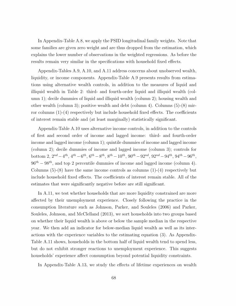
In Appendix-Table A.8, we apply the PSID longitudinal family weights. Note that

some families are given zero weight and are thus dropped from the estimation, which

explains the lower number of observations in the weighted regressions. As before the

results remain very similar in the specifications with household fixed e↵ects.

Appendix-Tables A.9, A.10, and A.11 address concerns about unobserved wealth,

liquidity, or income components. Appendix-Table A.9 presents results from estima-

tions using alternative wealth controls, in addition to the measures of liquid and

illiquid wealth in Table 2: third- and fourth-order liquid and illiquid wealth (col-

umn 1); decile dummies of liquid and illiquid wealth (column 2); housing wealth and

other wealth (column 3); positive wealth and debt (column 4). Columns (5)-(8) mir-

ror columns (1)-(4) respectively but include household fixed e↵ects. The coe�cients

of interest remain stable and (at least marginally) statistically significant.

Appendix-Table A.10 uses alternative income controls, in addition to the controls

of first and second order of income and lagged income: third- and fourth-order

income and lagged income (column 1); quintile dummies of income and lagged income

(column 2); decile dummies of income and lagged income (column 3); controls for

bottom 2, 2nd�4th, 4th�6th, 6th�8th, 8th�10th, 90th�92nd, 92nd�94th, 94th�96th,

96th � 98th, and top 2 percentile dummies of income and lagged income (column 4).

Columns (5)-(8) have the same income controls as columns (1)-(4) respectively but

include household fixed e↵ects. The coe�cients of interest remain stable. All of the

estimates that were significantly negative before are still significant.

In A.11, we test whether households that are more liquidity constrained are more

a↵ected by their unemployment experience. Closely following the practice in the

consumption literature such as Johnson, Parker, and Souleles (2006) and Parker,

Souleles, Johnson, and McClelland (2013), we sort households into two groups based

on whether their liquid wealth is above or below the sample median in the respective

year. We then add an indicator for below-median liquid wealth as well as its inter-

actions with the experience variables to the estimating equation (3). As Appendix-

Table A.11 shows, households in the bottom half of liquid wealth tend to spend less,

but do not exhibit stronger reactions to unemployment experience. This suggests

households’ experience a↵ect consumption beyond potential liquidity constraints.

In Appendix-Table A.13, we study the e↵ects of lifetime experiences on wealth

68

accumulation. This analysis tests whether, given the significant impact of unem-

ployment experiences on consumption, we can also detect experience e↵ects in the

build-up of wealth. The dependent variables are either liquid wealth or total wealth,

and the main regressors are lagged experience measures. We lag the experience mea-

sures by six, eight, ten, twelve, and 14 years, instead of using the contemporary

experience measures, recognizing that the e↵ects of experience on wealth may take

time to realize. We include the same set of control variables as in our main analyses,

including controls for income in years t� 1 and t� 2, and add a control for the av-

erage family income between year t� 2 and the year in which the lagged experience

measures are based on (six, eight, ten, twelve, and 14 years ago, respectively). For

example, when six-year lagged experience is the main regressor, we control for the

average income between t� 2 and t� 6. This average-income control addresses the

concern that previous experiences of economic boom or crisis may have implications

for future income (Oyer (2008); Kahn (2010); Oreopoulos, von Wachter, and Heisz

(2012)).35 In Appendix-Figure A.1, we plot the estimated coe�cients on the lagged

experience measures. In Appendix-Table A.13, we show the estimates of the coef-

ficients on the 10-year, 12-year, and 14-year lagged experience measures. We find

a significant role of past experiences for the build-up of wealth and liquid wealth,

especially in the context of personal experiences.

35 The results are similar if, instead of having an average-income control, we include the incomesfor all years between year t� 2 and the year in which the lagged experience measures are based on.

69

Table A.1: Summary Statistics (PSID), Full Sample

Variable Mean SD p10 p50 p90 NAge 47.65 12.03 32 47 65 37,156Experience (Macro) [in %] 6.00 0.28 5.67 5.97 6.37 37,156Experience (Personal) [in %] 5.77 16.57 0.00 0.00 20.00 37,156Household Size 2.73 1.45 1 2 5 37,156Household Food Consumption [in $] 8,559 5,630 2,600 7,608 15,451 37,156Household Total Consumption [in $] 46,256 36,497 14,733 39,559 82,765 37,156Household Total Income [in $] 93k 133k 17k 69k 178k 37,156Household Liquid Wealth [in $] 65k 718k -22k 0k 117k 37,156Household Illiquid Wealth [in $] 282k 1,268k 0k 72k 606k 37,156Household Total Wealth [in $] 346k 1,545k -3k 73k 762k 37,156

Notes. Summary statistics for the estimation sample, which covers the 1999-2013 PSID waves. Age,Experience (Macro), and Experience (Personal) are calculated for the heads of households. Household totalincome includes transfers and taxable income of all household members from the last year. Liquid wealthand illiquid wealth are defined following Kaplan, Violante and Weidner (2014). All values are in 2013 dollarsusing the PCE. Observations are annual and not weighted.

70

Table A.2: Consumption (PSID), Full Sample

(1) (2) (3) (4) (5) (6)Dependent Variable: Food ConsumptionExperience (Macro) -0.181*** -0.165*** -0.171** -0.163**

(0.051) (0.050) (0.069) (0.069)Experience (Personal) -0.756*** -0.752*** -0.426*** -0.422***

(0.114) (0.114) (0.137) (0.137)

R-squared 0.199 0.204 0.204 0.542 0.543 0.543Dependent Variable: Total ConsumptionExperience (Macro) -0.059* -0.046 -0.079** -0.073**

(0.031) (0.028) (0.031) (0.031)Experience (Personal) -0.603*** -0.602*** -0.328*** -0.326***

(0.073) (0.073) (0.082) (0.082)

R-squared 0.496 0.507 0.507 0.755 0.757 0.757Demographic controls Yes Yes Yes Yes Yes YesIncome controls Yes Yes Yes Yes Yes YesWealth controls Yes Yes Yes Yes Yes YesAge fixed e↵ects Yes Yes Yes Yes Yes YesState fixed e↵ects Yes Yes Yes Yes Yes YesYear fixed e↵ects Yes Yes Yes Yes Yes YesHousehold fixed e↵ects No No No Yes Yes Yes

Observations 37,156 37,156 37,156 37,156 37,156 37,156

Notes. We include all observations i.e., also observations with total family income below the 5th or abovethe 95th percentile in each wave from 1999 to 2013, as well as the pre-sample 1997 wave (because we controlfor lagged income). All variables are defined as in Table 2. Robust standard errors (in parentheses) areclustered by cohort. *, **, *** denote 10%, 5%, and 1% significance, respectively.

71

Table A.3: Consumption (PSID), Alternative Experience Measure: Gap Years

(1) (2) (3) (4) (5) (6)Dependent Variable: Food ConsumptionExperience (Macro) -0.099** -0.093* -0.124** -0.120**

(0.047) (0.048) (0.055) (0.055)Experience (Personal) -0.337*** -0.335*** -0.267** -0.264**

(0.104) (0.104) (0.127) (0.128)

R-squared 0.192 0.193 0.193 0.541 0.542 0.542Dependent Variable: Total ConsumptionExperience (Macro) -0.022 -0.018 -0.061*** -0.059***

(0.020) (0.019) (0.022) (0.022)Experience (Personal) -0.182*** -0.181*** -0.152*** -0.151***

(0.031) (0.031) (0.033) (0.033)

R-squared 0.573 0.574 0.574 0.788 0.788 0.788

Demographic controls Yes Yes Yes Yes Yes YesIncome controls Yes Yes Yes Yes Yes YesWealth controls Yes Yes Yes Yes Yes YesAge fixed e↵ects Yes Yes Yes Yes Yes YesState fixed e↵ects Yes Yes Yes Yes Yes YesYear fixed e↵ects Yes Yes Yes Yes Yes YesHousehold fixed e↵ects No No No Yes Yes Yes

Observations 33,164 33,164 33,164 33,164 33,164 33,164

Notes. All variables other than the experience measures are defined as in Table 2. The construction of theexperience measures di↵ers as follows: For any gap year t (between PSID survey waves in t� 1 and t+ 1),the baseline experience measures in the main text assume that families reside in the same state as in yeart� 1. The alternative construction used in this Appendix-Table assumes that families reside half of year t intheir (t-1)-state of residence, and half of the year in their (t+1)-state of residence. (The di↵erent assumptiondoes not matter when a family does not move between surveys.) Hence, the macro experience measure inthis Appendix-Table uses the average of the year t unemployment rates of the (t-1)-state of residence andthe (t+1)-state residence as gap year t’s unemployment rate. Similarly, for the personal experience measure,we fill in the employment status of a household head in a gap year with the average of the years before andafter. For example, if a person is unemployed in t� 1 and is employed in t+1, then his personal experiencein year t is denoted as 0.5. We exclude from the sample observations with total family income below the 5th

or above the 95th percentile in each wave from 1999 to 2013, as well as the pre-sample 1997 wave (becausewe control for lagged income). Robust standard errors (in parentheses) are clustered by cohort. *, **, ***denote 10%, 5%, and 1% significance, respectively.

72

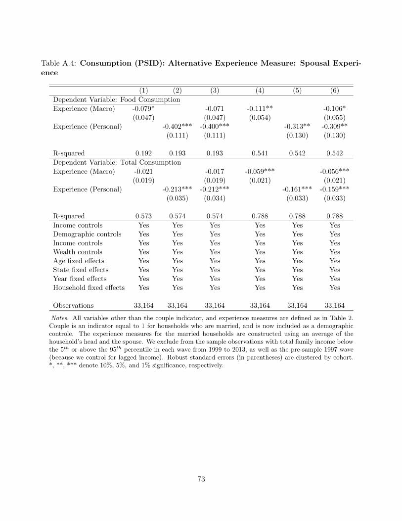
Table A.4: Consumption (PSID): Alternative Experience Measure: Spousal Experi-ence

(1) (2) (3) (4) (5) (6)Dependent Variable: Food ConsumptionExperience (Macro) -0.079* -0.071 -0.111** -0.106*

(0.047) (0.047) (0.054) (0.055)Experience (Personal) -0.402*** -0.400*** -0.313** -0.309**

(0.111) (0.111) (0.130) (0.130)

R-squared 0.192 0.193 0.193 0.541 0.542 0.542Dependent Variable: Total ConsumptionExperience (Macro) -0.021 -0.017 -0.059*** -0.056***

(0.019) (0.019) (0.021) (0.021)Experience (Personal) -0.213*** -0.212*** -0.161*** -0.159***

(0.035) (0.034) (0.033) (0.033)

R-squared 0.573 0.574 0.574 0.788 0.788 0.788Income controls Yes Yes Yes Yes Yes YesDemographic controls Yes Yes Yes Yes Yes YesIncome controls Yes Yes Yes Yes Yes YesWealth controls Yes Yes Yes Yes Yes YesAge fixed e↵ects Yes Yes Yes Yes Yes YesState fixed e↵ects Yes Yes Yes Yes Yes YesYear fixed e↵ects Yes Yes Yes Yes Yes YesHousehold fixed e↵ects Yes Yes Yes Yes Yes Yes

Observations 33,164 33,164 33,164 33,164 33,164 33,164

Notes. All variables other than the couple indicator, and experience measures are defined as in Table 2.Couple is an indicator equal to 1 for households who are married, and is now included as a demographiccontrole. The experience measures for the married households are constructed using an average of thehousehold’s head and the spouse. We exclude from the sample observations with total family income belowthe 5th or above the 95th percentile in each wave from 1999 to 2013, as well as the pre-sample 1997 wave(because we control for lagged income). Robust standard errors (in parentheses) are clustered by cohort.*, **, *** denote 10%, 5%, and 1% significance, respectively.

73

Table A.5: Consumption (PSID), Alternative Experience Measure: Lagged Experi-ence

Dependent Varariable: Food Consumption Total Consumption(1) (2) (3) (4) (5) (6)

Dependent Variable: Food ConsumptionExperience (Macro) -0.109* -0.103* -0.094** -0.093**

(0.056) (0.057) (0.046) (0.046)Experience (Personal) -0.320** -0.318** -0.066 -0.064

(0.134) (0.134) (0.136) (0.136)

R-squared 0.204 0.205 0.205 0.587 0.587 0.587Dependent Variable: Total ConsumptionExperience (Macro) -0.013 -0.010 -0.047* -0.046*

(0.024) (0.024) (0.026) (0.025)Experience (Personal) -0.179*** -0.178*** -0.120*** -0.119***

(0.038) (0.038) (0.038) (0.038)

R-squared 0.572 0.573 0.573 0.806 0.807 0.807

Income controls Yes Yes Yes Yes Yes YesDemographic controls Yes Yes Yes Yes Yes YesIncome controls Yes Yes Yes Yes Yes YesWealth controls Yes Yes Yes Yes Yes YesAge fixed e↵ects Yes Yes Yes Yes Yes YesState fixed e↵ects Yes Yes Yes Yes Yes YesYear fixed e↵ects Yes Yes Yes Yes Yes YesHousehold fixed e↵ects Yes Yes Yes Yes Yes Yes

Observations 20,163 20,163 20,163 20,163 20,163 20,163

Notes. The experience measures (both macro and personal) does not contain unemployment experiencefrom year t � 1. All other variables are defined as in Table 2. We exclude from the sample observationswith total family income below the 5th or above the 95th percentile in each wave from 1999 to 2013, aswell as the pre-sample 1997 wave (because we control for lagged income). Robust standard errors (inparentheses) are clustered by cohort. *, **, *** denote 10%, 5%, and 1% significance, respectively.

74

Table A.6: Consumption (PSID), Alternative Experience Measure: Di↵er-ent Weights (� = 3)

Dependent Varariable: Food Consumption Total Consumption(1) (2) (3) (4) (5) (6)

Experience (Macro) -0.021** -0.019* -0.033*** -0.032**(0.010) (0.011) (0.012) (0.012)

Experience (Personal) -0.175*** -0.174*** -0.150*** -0.149***(0.029) (0.029) (0.031) (0.031)

R-squared 0.573 0.574 0.574 0.788 0.788 0.788Demographic controls Yes Yes Yes Yes Yes YesIncome controls Yes Yes Yes Yes Yes YesWealth controls Yes Yes Yes Yes Yes YesAge fixed e↵ects Yes Yes Yes Yes Yes YesState fixed e↵ects Yes Yes Yes Yes Yes YesYear fixed e↵ects Yes Yes Yes Yes Yes YesHousehold fixed e↵ects Yes Yes Yes Yes Yes Yes

Observations 33,164 33,164 33,164 33,164 33,164 33,164

Notes. All variables other than the experience measures are defined as in Table 2. The experience measuresare constructed using � = 0 in the upper part of the table, and � = 3 in the lower part. We exclude from thesample observations with total family income below the 5th or above the 95th percentile in each wave from1999 to 2013, as well as the pre-sample 1997 wave (because we control for lagged income). Robust standarderrors (in parentheses) are clustered by cohort. *, **, *** denote 10%, 5%, and 1% significance, respectively.

75

Tab

leA.7:Consu

mption

(PSID

),AlternativeClusteringUnits

(1)

(2)

(3)

(4)

(5)

(6)

(7)

(8)

Dep

endentVariable:Foo

dCon

sumption

Exp

erience

(Macro)

-0.091

**-0.091

**-0.091

**-0.091

**-0.117

**-0.117

-0.117

**-0.117

**(0.041

)(0.033

)(0.046

)(0.042

)(0.053

)(0.062

)(0.050

)(0.049

)Exp

erience

(Personal)

-0.320

***

-0.320

**-0.320

***

-0.320

***

-0.260

**-0.260

*-0.260

***

-0.260

**(0.086

)(0.113

)(0.095

)(0.085

)(0.109

)(0.132

)(0.099

)(0.101

)

R-squ

ared

0.19

30.19

30.19

30.19

30.54

20.54

20.54

20.54

2Dep

endentVariable:Total

Con

sumption

Exp

erience

(Macro)

-0.018

-0.018

-0.018

-0.018

-0.057

***

-0.057

**-0.057

***

-0.057

***

(0.015

)(0.017

)(0.017

)(0.015

)(0.017

)(0.020

)(0.019

)(0.017

)Exp

erience

(Personal)

-0.177

***

-0.177

***

-0.177

***

-0.177

***

-0.147

***

-0.147

**-0.147

***

-0.147

***

(0.024

)(0.046

)(0.026

)(0.023

)(0.028

)(0.043

)(0.030

)(0.027

)

R-squ

ared

0.57

40.57

40.57

40.57

40.78

80.78

80.78

80.78

8Dem

ographic

controls

Yes

Yes

Yes

Yes

Yes

Yes

Yes

Yes

Incomecontrols

Yes

Yes

Yes

Yes

Yes

Yes

Yes

Yes

Wealthcontrols

Yes

Yes

Yes

Yes

Yes

Yes

Yes

Yes

Age

fixede↵

ects

Yes

Yes

Yes

Yes

Yes

Yes

Yes

Yes

Yearfixede↵

ects

Yes

Yes

Yes

Yes

Yes

Yes

Yes

Yes

State

fixede↵

ects

Yes

Yes

Yes

Yes

Yes

Yes

Yes

Yes

Hou

seholdfixede↵

ects

No

No

No

No

Yes

Yes

Yes

Yes

Observations

33,164

33,164

33,164

33,164

33,164

33,164

33,164

33,164

Notes.Allvariab

lesaredefined

asin

Tab

le2.

Standarderrors

incolumns(1)to

(4)areclustered

bycohort⇤year,cohortan

dyear

(two-way

clustering),hou

seholdan

dhou

sehold⇤year,

respectively,an

dthesameforcolumns(5)to

(8).

Weexcludefrom

thesample

observationswith

totalfamilyincomebelow

the5t

hor

abovethe95

thpercentilein

each

wavefrom

1999

to2013,as

wellas

the

pre-sam

ple

1997

wave(becau

sewecontrolforlagged

income).Rob

ust

stan

darderrors

(inparentheses)areclustered

bycohort.

*,**,

***denote10%,5%

,an

d1%

sign

ificance,respectively.

76

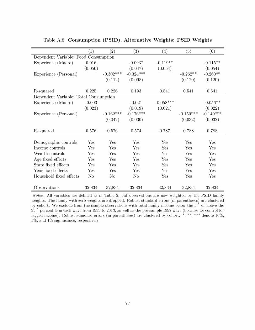
Table A.8: Consumption (PSID), Alternative Weights: PSID Weights

(1) (2) (3) (4) (5) (6)Dependent Variable: Food ConsumptionExperience (Macro) 0.016 -0.093* -0.119** -0.115**

(0.056) (0.047) (0.054) (0.054)Experience (Personal) -0.302*** -0.324*** -0.262** -0.260**

(0.112) (0.098) (0.120) (0.120)

R-squared 0.225 0.226 0.193 0.541 0.541 0.541Dependent Variable: Total ConsumptionExperience (Macro) -0.003 -0.021 -0.058*** -0.056**

(0.023) (0.019) (0.021) (0.022)Experience (Personal) -0.162*** -0.176*** -0.150*** -0.149***

(0.042) (0.030) (0.032) (0.032)

R-squared 0.576 0.576 0.574 0.787 0.788 0.788

Demographic controls Yes Yes Yes Yes Yes YesIncome controls Yes Yes Yes Yes Yes YesWealth controls Yes Yes Yes Yes Yes YesAge fixed e↵ects Yes Yes Yes Yes Yes YesState fixed e↵ects Yes Yes Yes Yes Yes YesYear fixed e↵ects Yes Yes Yes Yes Yes YesHousehold fixed e↵ects No No No Yes Yes Yes

Observations 32,834 32,834 32,834 32,834 32,834 32,834

Notes. All variables are defined as in Table 2, but observations are now weighted by the PSID familyweights. The family with zero weights are dropped. Robust standard errors (in parentheses) are clusteredby cohort. We exclude from the sample observations with total family income below the 5th or above the95th percentile in each wave from 1999 to 2013, as well as the pre-sample 1997 wave (because we control forlagged income). Robust standard errors (in parentheses) are clustered by cohort. *, **, *** denote 10%,5%, and 1% significance, respectively.

77

Tab

leA.9:Consu

mption

(PSID

),AdditionalW

ealth

Controls

(1)

(2)

(3)

(4)

(5)

(6)

(7)

(8)

Dep

endentVariable:Foo

dCon

sumption

Exp

erience

(Macro)

-0.088

*-0.079

-0.082

*-0.082

-0.110

**-0.101

*-0.104

*-0.096

*(0.047

)(0.047

)(0.048

)(0.051

)(0.054

)(0.054

)(0.054

)(0.055

)Exp

erience

(Personal)

-0.318

***

-0.272

***

-0.321

***

-0.231

**-0.258

**-0.258

**-0.261

**-0.226

*(0.097

)(0.099

)(0.098

)(0.098

)(0.119

)(0.120

)(0.119

)(0.120

)

R-squ

ared

0.19

40.19

90.19

40.20

30.54

20.54

30.54

20.55

1Dep

endentVariable:Total

Con

sumption

Exp

erience

(Macro)

-0.015

-0.005

-0.013

-0.003

-0.054

**-0.046

**-0.053

**-0.040

*(0.019

)(0.019

)(0.019

)(0.020

)(0.021

)(0.021

)(0.022

)(0.020

)Exp

erience

(Personal)

-0.175

***

-0.131

***

-0.178

***

-0.069

***

-0.146

***

-0.144

***

-0.148

***

-0.130

***

(0.029

)(0.026

)(0.029

)(0.024

)(0.031

)(0.030

)(0.031

)(0.030

)

R-squ

ared

0.57

70.59

60.57

50.63

30.78

80.79

10.78

80.80

5

Dem

ographic

controls

Yes

Yes

Yes

Yes

Yes

Yes

Yes

Yes

Wealthcontrols

Yes

Yes

Yes

Yes

Yes

Yes

Yes

Yes

Age

fixede↵

ects

Yes

Yes

Yes

Yes

Yes

Yes

Yes

Yes

Yearfixede↵

ects

Yes

Yes

Yes

Yes

Yes

Yes

Yes

Yes

State

fixede↵

ects

Yes

Yes

Yes

Yes

Yes

Yes

Yes

Yes

Hou

seholdfixede↵

ects

No

No

No

No

Yes

Yes

Yes

Yes

Observations

33,164

33,164

33,164

31,187

33,164

33,164

33,164

31,187

Notes.Regressionsdi↵er

from

thosein

Tab

le2on

lyin

term

sof

thewealthcontrols.Column(1)controls

forthird-an

dfourth-order

liqu

idan

dilliqu

idwealth.Column(2)includes

deciledummiesof

liqu

idwealthan

dilliqu

idwealth.Column(3)controls

forhou

sing

wealthan

dother

wealth(total

wealthminushou

singwealth).

Column(4)controls

forpositivewealthan

ddebt.

Allwealthcontrols

arein

additionto

thecontrols

offirstan

dsecondorder

ofliqu

idan

dilliqu

idwealth.Columns(5)–(8)havethesamewealthcontrols

ascolumns(1)–(4)respectively.Rob

ust

stan

darderrors

areclustered

bycohort.

*,**,***denote10%,5%

,an

d1%

sign

ificance,

respectively.

78

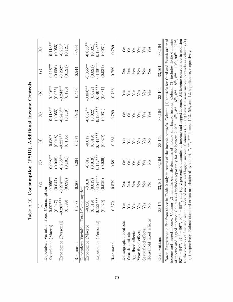
Tab

leA.10:

Consu

mption

(PSID

),AdditionalIn

comeControls

(1)

(2)

(3)

(4)

(5)

(6)

(7)

(8)

Dep

endentVariable:Foo

dCon

sumption

Exp

erience

(Macro)

-0.097

**-0.095

**-0.098

**-0.089

*-0.118

**-0.116

**-0.118

**-0.113

**(0.047

)(0.047

)(0.048

)(0.048

)(0.055

)(0.055

)(0.056

)(0.055

)Exp

erience

(Personal)

-0.267

***

-0.274

***

-0.238

**-0.227

**-0.240

**-0.243

**-0.232

*-0.233

*(0.099

)(0.098

)(0.101

)(0.105

)(0.119

)(0.120

)(0.121

)(0.121

)

R-squ

ared

0.20

00.20

00.20

40.20

60.54

30.54

30.54

40.54

4Dep

endentVariable:Total

Con

sumption

Exp

erience

(Macro)

-0.020

-0.018

-0.017

-0.017

-0.057

**-0.056

**-0.056

**-0.056

**(0.019

)(0.019

)(0.019

)(0.019

)(0.022

)(0.022

)(0.021

)(0.021

)Exp

erience

(Personal)

-0.153

***

-0.154

***

-0.142

***

-0.141

***

-0.139

***

-0.140

***

-0.136

***

-0.138

***

(0.029

)(0.029

)(0.029

)(0.029

)(0.031

)(0.031

)(0.031

)(0.031

)

R-squ

ared

0.57

90.57

90.58

10.58

10.78

90.78

80.78

90.78

9

Dem

ographic

controls

Yes

Yes

Yes

Yes

Yes

Yes

Yes

Yes

Wealthcontrols

Yes

Yes

Yes

Yes

Yes

Yes

Yes

Yes

Age

fixede↵

ects

Yes

Yes

Yes

Yes

Yes

Yes

Yes

Yes

Yearfixede↵

ects

Yes

Yes

Yes

Yes

Yes

Yes

Yes

Yes

State

fixede↵

ects

Yes

Yes

Yes

Yes

Yes

Yes

Yes

Yes

Hou

seholdfixede↵

ects

No

No

No

No

Yes

Yes

Yes

Yes

Observations

33,164

33,164

33,164

33,164

33,164

33,164

33,164

33,164

Notes.Regressionsdi↵er

from

thosein

Tab

le2on

lyin

term

sof

theincomecontrols.Column(1)controlsforthirdan

dfourthorder

ofincomean

dlagged

income.

Column(2)includes

quintile

dummiesof

incomean

dlagged

income.

Column(3)includes

deciledummies

ofincomean

dlagged

income.

Column(4)includes

separatelyforthebottom

2,2n

d�4t

h,4t

h�6t

h,6t

h�8t

h,8t

h�10

th,90

th�92

nd,

92nd�

94th,94

th�

96th,96

th�

98th,an

dtop2percentiledummiesof

incomean

dlagged

income.

Allincomecontrols

arein

addition

tothecontrolsof

firstan

dsecondorder

ofincomean

dlagged

income.

Columns(5)–(8)havethesameincomecontrolsas

columns(1)

–(4)respectively.Rob

ust

stan

darderrors

areclustered

bycohort.

*,**,***denote10%,5%

,an

d1%

sign

ificance,respectively.

79

Table A.11: Consumption (PSID), Additional Liquidity Controls

(1) (2) (3) (4) (5) (6)Dependent Variable: Food ConsumptionExperience (Macro) -0.147** -0.144** -0.143** -0.143**

(0.058) (0.058) (0.063) (0.063)Experience (Macro) * LLW 0.097 0.103* 0.048 0.055

(0.060) (0.059) (0.056) (0.055)Low Liquid Wealth -0.572 0.013 -0.602* -0.316 -0.023 -0.352

(0.358) (0.013) (0.355) (0.335) (0.014) (0.331)Experience (Personal) -0.302** -0.292** -0.241 -0.236

(0.142) (0.142) (0.149) (0.149)Experience (Personal) * LLW -0.037 -0.053 -0.038 -0.046

(0.177) (0.176) (0.156) (0.155)

R-squared 0.192 0.193 0.193 0.542 0.542 0.542Dependent Variable: Total ConsumptionExperience (Macro) -0.021 -0.023 -0.054** -0.055**

(0.022) (0.022) (0.024) (0.023)Experience (Macro) * LLW 0.001 0.009 -0.012 -0.006

(0.015) (0.016) (0.015) (0.016)Low Liquid Wealth 0.034 0.047*** -0.006 0.080 0.013*** 0.046

(0.093) (0.006) (0.094) (0.093) (0.004) (0.095)Experience (Personal) -0.087** -0.086** -0.083** -0.082**

(0.036) (0.036) (0.033) (0.033)Experience (Personal) * LLW -0.166*** -0.168*** -0.118*** -0.118***

(0.046) (0.046) (0.044) (0.044)

R-squared 0.573 0.575 0.575 0.788 0.788 0.788Demographic controls Yes Yes Yes Yes Yes YesIncome controls Yes Yes Yes Yes Yes YesWealth controls Yes Yes Yes Yes Yes YesAge fixed e↵ects Yes Yes Yes Yes Yes YesState fixed e↵ects Yes Yes Yes Yes Yes YesYear fixed e↵ects Yes Yes Yes Yes Yes YesHousehold fixed e↵ects No No No Yes Yes Yes

Observations 33,164 33,164 33,164 33,164 33,164 33,164

Notes. Low Liquid Wealth (LLW) is an indicator variable equal to 1 for households with liquid wealthbelow the sample-year median. All other variables are defined as in Table 2. We exclude from the sampleobservations with total family income below the 5th or above the 95th percentile in each wave from 1999 to2013, as well as the pre-sample 1997 wave (because we control for lagged income). Robust standard errors(in parentheses) are clustered by cohort. *, **, *** denote 10%, 5%, and 1% significance, respectively.

80

Tab

leA.12:

Experience

E↵ec

tsand

Futu

reIn

comeVolatility

Dep

endentVariable:Variance

ofIncome

(1)

(2)

(3)

(4)

(5)

(6)

Perman

ent t+2

Transitory

t+2

Perman

ent t+4

Transitory

t+4

Perman

ent t+6

Transitory

t+6

Exp

erience

(Macro)

0.08

4*0.02

50.03

90.14

00.07

00.16

1(0.049

)(0.074

)(0.051

)(0.095

)(0.068

)(0.104

)Exp

erience

(Personal)

0.11

2-0.031

0.03

3-0.175

0.13

8-0.062

(0.164

)(0.159

)(0.134

)(0.157

)(0.110

)(0.187

)

Observations

15,665

28,410

15,665

21,082

11,196

15,713

R-squ

ared

0.41

00.36

40.38

90.37

90.43

70.24

8Dem

ographic

controls

Yes

Yes

Yes

Yes

Yes

Yes

Incomecontrols

Yes

Yes

Yes

Yes

Yes

Yes

Wealthcontrols

Yes

Yes

Yes

Yes

Yes

Yes

State

fixede↵

ects

Yes

Yes

Yes

Yes

Yes

Yes

Yearfixede↵

ects

Yes

Yes

Yes

Yes

Yes

Yes

Hou

seholdfixede↵

ects

Yes

Yes

Yes

Yes

Yes

Yes

Observations

12,201

24,060

12,201

17,072

8,41

612

,573

R-squ

ared

0.39

60.33

40.39

50.45

20.41

90.44

3

Notes.Thedep

endentvariab

lesareperman

entan

dtran

sitory

incomevolatility

intw

o,four,

andsixyears,

respectively.”E

xperience

(Macro)”

isthemacroecon

omic

experience

measure

ofunem

ploym

ent,

and”E

xperience

(Personal)”

isthepersonal

experience

measure.

Dem

ographic

controls

includefamilysize,heads’

gender,race,marital

status,

education

level,an

dadummyvariab

leindicatingwhether

therespon

dentis

unem

ployedat

thetimeof

thesurvey.Incomecontrols

includethefirstan

dsecondorder

ofthelogarithm

ofincome

andlagg

edincome.

Wealthcontrols

includethefirstan

dsecondorder

ofthelogarithm

ofliqu

idan

dilliqu

idwealth.Weexcludefrom

thesample

observationswithtotalfamilyincomebelow

the5t

hor

abovethe95

thpercentilein

each

wavefrom

1999

to2013,as

wellas

thepre-sam

ple

1997

wave(becau

sewecontrolforlagged

income).Wetake

thelogarithm

ofincome,

andwealth;non

-positivevalues

are

adjusted

byad

dingtheab

solute

valueof

theminim

um

plus0.1beforebeinglogarithmized.Rob

ust

stan

darderrors

(inparentheses)are

clustered

bycohort.

*,**,***denote10%,5%

,an

d1%

sign

ificance,respectively.

81

Tab

leA.13:

Wea

lth

Acc

umulation

Dep

endentVar.:

Liquid

Wealthat

timet

Total

Wealthat

timet

(1)

(2)

(3)

(4)

(5)

(6)

(7)

(8)

(9)

(10)

(11)

(12)

Exp

.(M

acro) t�10

0.006*

0.005

0.003

0.003

0.012

0.010

0.018***

0.019***

(0.003)

(0.003)

(0.003)

(0.003)

(0.008)

(0.008)

(0.006)

(0.006)

Exp

.(P

ersonal) t�10

0.023***

0.023***

-0.000

-0.001

0.083***

0.083***

-0.003

-0.005

(0.004)

(0.004)

(0.002)

(0.002)

(0.013)

(0.013)

(0.014)

(0.014)

R-squ

ared

0.048

0.048

0.048

0.332

0.332

0.332

0.292

0.294

0.294

0.714

0.714

0.714

Observations

21,691

21,691

21,691

21,691

21,691

21,691

21,691

21,691

21,691

21,691

21,691

21,691

Exp

.(M

acro) t�12

0.007**

0.006*

0.008**

0.007**

0.010

0.007

0.020***

0.020***

(0.003)

(0.003)

(0.003)

(0.003)

(0.009)

(0.009)

(0.007)

(0.007)

Exp

.(P

ersonal) t�12

0.026***

0.026***

0.002

0.001

0.092***

0.091***

0.003

0.001

(0.005)

(0.005)

(0.002)

(0.003)

(0.014)

(0.014)

(0.014)

(0.014)

R-squ

ared

0.049

0.050

0.050

0.333

0.333

0.333

0.294

0.296

0.296

0.730

0.730

0.730

Observations

19,427

19,427

19,427

19,427

19,427

19,427

19,427

19,427

19,427

19,427

19,427

19,427

Exp

.(M

acro) t�14

0.008**

0.007*

0.008**

0.008**

0.002

-0.001

0.011*

0.010

(0.003)

(0.003)

(0.003)

(0.003)

(0.009)

(0.010)

(0.006)

(0.006)

Exp

.(P

ersonal) t�14

0.028***

0.028***

0.003

0.002

0.095***

0.095***

0.010

0.009

(0.005)

(0.005)

(0.003)

(0.003)

(0.013)

(0.013)

(0.009)

(0.009)

R-squ

ared

0.052

0.052

0.052

0.331

0.331

0.331

0.378

0.380

0.380

0.827

0.827

0.827

Observations

17,151

17,151

17,151

17,151

17,151

17,151

17,151

17,151

17,151

17,151

17,151

17,151

Dem

ographic

controls

Yes

Yes

Yes

Yes

Yes

Yes

Yes

Yes

Yes

Yes

Yes

Yes

Incomecontrols

Yes

Yes

Yes

Yes

Yes

Yes

Yes

Yes

Yes

Yes

Yes

Yes

Age

fixede↵

ects

Yes

Yes

Yes

Yes

Yes

Yes

Yes

Yes

Yes

Yes

Yes

Yes

State

fixede↵

ects

Yes

Yes

Yes

Yes

Yes

Yes

Yes

Yes

Yes

Yes

Yes

Yes

Yearfixede↵

ects

Yes

Yes

Yes

Yes

Yes

Yes

Yes

Yes

Yes

Yes

Yes

Yes

Hou

seholdfixede↵

ects

No

No

No

Yes

Yes

Yes

No

No

No

Yes

Yes

Yes

Notes.“E

xp.(M

acro)”

isthemacroecon

omic

experience

measure,an

d“E

xp.(P

ersonal)”

isthepersonal

experience

measure.Liquid

wealthan

dtotal

wealtharedefined

asin

themaindraft.Weseparatelyuse

thet�

10,t�

12experience

measures,

andt�

14experience

measures.

Incomecontrols

include

thet�

1familytotalincomean

dtheaveragefamilytotalincomebetweent�

2an

dtheyear

weuse

theexperience

measures.

For

gapyearsbetweenPSID

survey

waves,weuse

prior-yearincome.

Dem

ographic

controls

includefamilysize,thehou

seholdheads’

gender,race,marital

status,

education

level,an

dem

ploym

entstatus.

Wetake

theloga

rithm

ofallincomean

dwealthvariab

les.

Rob

ust

stan

darderrors

(inparentheses)areclustered

bycohort.

*,**,***

denote10%,5%

,an

d1%

sign

ificance,respectively.

82

A.2 Robustness using CEX-Nielsen Synthetic Panel Data

In order to keep the advantages of panel analysis but also exploit the comprehensive-

ness of the CEX, we match the two datasets and create a synthetic panel. Specifically,

we match a CEX household i with a Nielsen household j on a set of common co-

variates (characteristics) xi = (xi,1, xi,2, ..., xi,p) and xj = (xj,1, xj,2, ..., xj,p), which

include age, income, marital status, household size, education, race, region of resi-

dency, employment status, as well as their consumption of non-durable items, using

the nearest-neighbor matching estimator from Rosenbaum and Rubin (1983) and

Abadie and Imbens (2011). The distance between xi and xj is the vector norm

k xi � xj kS= ((xi � xj)0S�1(xi � xj))1/2, where S is a symmetric, positive-definite

matrix. We find the set of nearest-neighbor indices for observation i in the CEX as

⌦i = (j|tj = 1� ti, k xi � xj kS<k xi � xl kS, tl = 1� ti, l 6= j) in Nielsen. In words,

the nearest-neighbor propensity-score matching chooses for each observation in the

CEX an observation in Nielsen that has the closest estimated propensity score.

Table A.14 provides summary statistics for the matched sample. In the matched

dataset, the distributions on total and durable consumption are comparable to those

of the underlying CEX data, which is indicative of successful matching. For an

average household, its share of durable consumption makes up 10% of total spending,

while non-durable consumption amounts to 69% of total spending.

Table A.14: Summary Statistics (Nielsen-CEX Matched Data)

Variable Mean SD p10 p50 p90 NTotal consumption expenditure 4,508 4,919 1,838 3,371 7,111 866,819Durable consumption 1,078 4,466 0 117 1,460 866,819Non-durable consumption 2,612 1,178 1,423 2,400 4,025 866,819Non-durable consumption (Nielsen) 2,139 1,602 618 1,757 4,083 3,171,833Experience (Macro) 5.9 0.2 5.8 5.9 6.2 866,819Notes. The sample period runs from 2004 to 2012. Observations are quarterly and not weighted.

Table A.15 shows results from re-estimating specification (11) using the matched

CEX-Nielsen sample. In columns (1) and (4), we use total expenditures as the

outcome variable, in columns (2) and (5) durable consumption spending, and in

columns (3) and (6) non-durables. As before we show the results both without

household fixed e↵ects (columns 1 to 3) and with fixed e↵ects (columns 4 to 6).

83

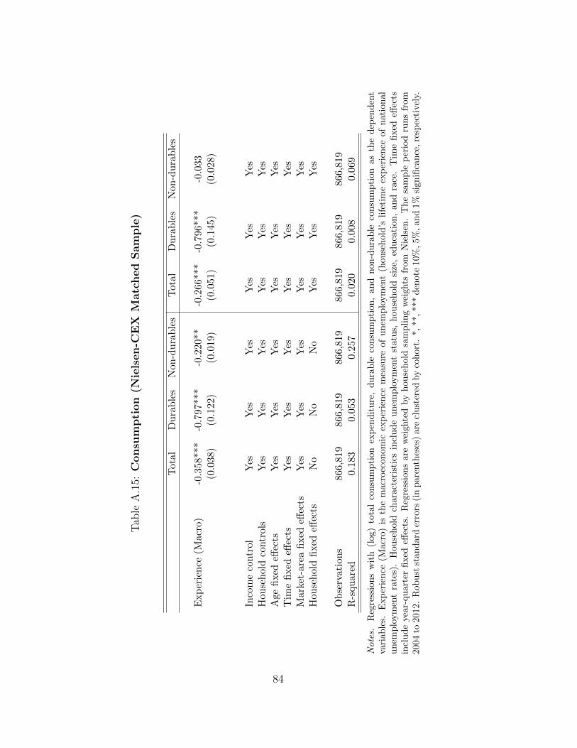
Tab

leA.15:

Consu

mption

(Nielsen

-CEX

Matched

Sample)

Total

Durables

Non

-durables

Total

Durables

Non

-durables

Exp

erience

(Macro)

-0.358

***

-0.797

***

-0.220

**-0.266

***

-0.796

***

-0.033

(0.038

)(0.122

)(0.019

)(0.051

)(0.145

)(0.028

)

Incomecontrol

Yes

Yes

Yes

Yes

Yes

Yes

Hou

seholdcontrols

Yes

Yes

Yes

Yes

Yes

Yes

Age

fixede↵

ects

Yes

Yes

Yes

Yes

Yes

Yes

Tim

efixede↵

ects

Yes

Yes

Yes

Yes

Yes

Yes

Market-area

fixede↵

ects

Yes

Yes

Yes

Yes

Yes

Yes

Hou

seholdfixede↵

ects

No

No

No

Yes

Yes

Yes

Observations

866,81

986

6,81

986

6,81

986

6,81

986

6,81

986

6,81

9R-squ

ared

0.18

30.05

30.25

70.02

00.00

80.06

9

Notes.

Regressionswith(log)totalconsumption

expenditure,durable

consumption

,an

dnon

-durable

consumption

asthedep

endent

variab

les.

Exp

erience

(Macro)is

themacroecon

omic

experience

measure

ofunem

ploym

ent(hou

sehold’s

lifetimeexperience

ofnational

unem

ploym

entrates).Hou

seholdcharacteristicsincludeunem

ploym

entstatus,

hou

seholdsize,education

,an

drace.Tim

efixede↵

ects

includeyear-quarterfixede↵

ects.Regressionsareweigh

tedby

hou

seholdsamplingweigh

tsfrom

Nielsen.Thesample

periodrunsfrom

2004

to2012.Rob

ust

stan

darderrors

(inparentheses)areclustered

bycohort.

*,**,***denote10%,5%

,an

d1%

sign

ificance,respectively.

84

For all outcome variables – durable, non-durable, and total consumption – we

continue to estimate highly significant negative experience e↵ects. Households that

have experienced worse unemployment conditions during their lifetime spend signif-

icantly less in total, and also specifically on durable and on non-durable items. One

exception is non-durables in the case where we identify only within household; here

the coe�cient becomes small and insignificant. Otherwise, the coe�cients are stable

across specifications, and the economic magnitudes are large: a one standard devia-

tion increase in lifetime unemployment experience is associated with a $38 decline in

monthly non-durable consumption and $108 decline in monthly total consumption

(using the estimates of columns 3 and 1 respectively). The new estimate for durable

consumption is large and highly significant across specifications. A one standard de-

viation increase in lifetime unemployment experience is associated with a $57 decline

in monthly durable consumption.

Appendix B Model

We implement the empirical model of Low, Meghir, and Pistaferri (2010) with a few

minor adjustments to our setting. All key equations are retained and, when possible,

all parameters are set to the same values. As in Low et al., some parameters are

set separately for high- and low-education groups, including the probability of job

destruction and job o↵ers.

B.1 Parameters governing the income process and utility

maximization

The utility function and lifetime expected utility are defined in equations (4) and (5)

in Section IV as U(c, P ) =(c⇥e⌘P )

1��

1�� and U(ci,t, Pi,t) + Et

hPLs=t+1 �

s�tU(ci,s, Pi,s)i,

respectively. In the simulations, we follow Low et al. and take risk aversion parameter

� = 1.5 from Attanasio and Weber (1995), use the estimates for ⌘ from their Table

2, and set the discount factor � = 1/R in the value function.

For the gross quarterly income wi,th, we also follow Low et al. in setting the

number of hours worked per quarter to h = 500. In the wage process lnwi,t =

dt + x0i,t + ui,t + ai,j,t0 , we recover the parameters ↵, �1, and �2 governing the

85

deterministic component, dt + x0i,t = ↵ + �1 · age + �2 · age2, from the parameters

in the Fortran code published alongside Low et al. In the permanent component

ui,t = ui,t�1 + ⇣i,t, ⇣i,t is i. i. d. normal with mean 0 and variance �2⇣ , and we use the

value of �⇣ given in Table 1 of Low et al.. The consumer-firm job match component,

ai,j,t0 , is drawn from a normal distribution with mean 0 and variance �2a, and we use

the value of �a given in Table 1 of Low et al..

We obtain the values for the probabilities of job destruction �, of a job o↵er when

employed (1 � �)�e, and of a job o↵er when unemployed �n from Table 2 in Low

et al. (2010). Note that, while the probability of job destruction is constant across

time for a given household, the probability of receiving a job o↵er varies depending

on whether or not an agent is employed.

B.2 Budget constraint

The intertemporal budget constraint for a working individual i in period t is given

byAi,t+1 = R [Ai,t � ci,t] + (wi,th(1� ⌧w)� Fi,t)Pi,t

+�Bi,tI

UIi,t (1� IDI

i,t ) +Di,tIDIi,t

�(1� Pi,t) + Ti,tI

Ti,t

where Ai,t is beginning-of-period-t assets, R is the interest factor, ⌧w a tax, F the

fixed cost of working, P an indicator for whether an individual is working, B are un-

employment benefits, D disability benefits, T food stamp benefits, c is consumption,

and the I variables are indicators of receiving the associated social insurance.

As in Low et al. (2010), we assume that individuals cannot borrow and thus

Ai,t � 0 8t. Also as in Low et al. (2010), we set r = .15 and define R = 1 + r. We

use the estimates for F from their Table 2. In Low et al. (2010), ⌧w is a variable of

interest and solved for, albeit as fixed percentage (not progressive or regressive). As

we do not focus on the value of social insurance programs, including the tax revenues

to be raised to fund them and their relation with consumption, we normalize ⌧w = 0.

During retirement individuals receive social security equal to the value of disabil-

ity, so the budget constraints simplifies to

Ai,t+1 = R [Ai,t +Di,t � ci,t] .

86

B.3 Social Insurance programs

As in Low et al. (2010), we implement three social insurance programs, unemploy-

ment insurance, food stamps, and disability insurance.

Unemployment Insurance. Unemployment Insurance is paid only during the

quarter following job destruction. Unemployment benefits are given by

Bi,t =

8<

:bwi,t�1h if bwi,t�1h < Bmax,

Bmax if bwi,t�1h � Bmax.

where b is the replacement ratio, and Bmax is the cap on unemployment benefits. We

set b = .75 as in Low et al. (2010) and Bmax to the value used in the associated code.

Food Stamps (Means-Tested Social Insurance). Defining gross income as

ygrossi,t = wi,thPi,t +�Bi,tI

UIi,t (1� IDI

i,t ) +Di,tIDIi,t

�(1� Pi,t),

and net income as

y = (1� ⌧w)ygross � d,

the amount of food stamps allocated to agent i in period t is

Ti,t =

8<

:T � .3⇥ yi,t if yi,t y

0 otherwise,

where T is a maximum payment and y is a poverty line. One important implication

of this definition is that there is no disincentive to hold assets. Adjusting to quarterly

values, we set T to the maximum food stamp allotment for a couple in the US in

1993, y to the maximum food stamp allotment for the US in 1993, and d to the

standard deduction for a couple in the US in 1993.

Disability. As in Low et al. (2010), individuals above 50 can apply for disability

when they are unemployed, and are accepted with a fixed probability of .5. If an

application is successful, disability becomes an absorbing state for the remainder of

the person’s working life. If a person is not accepted, they can only reapply in a

future bout of unemployment, after having worked again for at least one year. As a

87

disincentive to applying, the individual must be unemployed in both the period they

apply and the period after. We also impose that individuals must have a su�ciently

low u and not be working or have a job o↵er at the time of application. The formula

for disability benefits is

Di,t =

8>>>>>><

>>>>>>:

.9⇥ wi if wi a1

.9⇥ a1 + .32⇥ (wi � a1) if a1 < wi a2

.9⇥ a1 + .32⇥ (a2 � a1) + .15⇥ (wi � a2) if a2 < wi a3

.9⇥ a1 + .32⇥ (a2 � a1) + .15⇥ (a3 � a2) if wi > a3

where a1, a1, and a3 are fixed thresholds from legislation, and wi is the mean earnings

prior to application. Similar to Low et al. (2010), we assume wi can be approximated

using the agent’s value of ui,t at the time of application.

B.4 Implementation

Appendix-Table B.1 details all parameters referenced above and their sources. As

discussed, most values are obtained directly from Low et al. (2010), and some are

retrieved from examining the associated Fortran 90 code published with the paper.

In cases where we were unable to ascertain values in either source, as is the case for

several welfare values, we use actual values from 1993, the year in which the SIPP

survey used in Low et al. for hourly wage data begins. This is also the closest year

in the SIPP survey to the PSID data, and the values are consistent with the model

values.

When we combine the high- and low-education data, we use 70% low- and 30%

high-education observations, roughly corresponding to recent US census estimates of

those without and with a bachelor’s degree.36

Like Low et al. (2010), we solve the model numerically. In the last period, all

agents consume the entirety of their assets. We then iteratively solve backwards for

consumption and other relevant decisions that maximize the agents’ value functions.

Further details of the model solution can be found in Low et al. (2010).

36 The percent of the US population with at least a bachelor’s degree has increased over thelast three decades. It was closer to 25% in 2007 and 20% in 1995. We opted for the more recentestimates to err, if anything, on the side of a greater inclusion of high-education individuals.

88

Table B.1: Model Parameters Used in Simulations

Parameter Low Education High Education Source (from Low, Meghir,and Pistaferri (2010))

� 1.5 1.5 Text�a 0.226 0.229 Table 1�⇣ 0.095 0.106 Table 1P (⇣) .25 .25 Text� .049 .028 Table 2�e .67 .72 Table 2�n .76 .82 Table 2b .75 .75 Textr (yearly) .015 .015 Text� 1/(1 + r) 1/(1 + r) TextF 1088 1213 Table 2⌘ -.55 -.62 Table 2h 500 500 Textb .75 .75 TextUI Cap 3178 3178 CodeP(DisabilityAcceptance)

.5 .5 Text

a1 1203 1203 Codea2 7260 7260 Codea3 16638 16638 Code↵ 1.0583 .642 Code�1 .0486 .0829 Code�2 -0.0004816 -.0007768 CodeParameter Low Education High Education Sourced 6200/4 Standard couple deduction

in 1993a

y (6970+2460)/4 Actual poverty line in 1993for coupleb

T 203 ⇥ 3 Actual max food stamp al-lotment for US 1993c

a See https://web.archive.org/web/20190228193856/https://www.irs.gov/pub/irs-prior/f1040a--1993.pdf.

b See https://web.archive.org/web/20190228194017/https://aspe.hhs.gov/prior-hhs-poverty-guidelines-and-federal-register-references.

c See https://web.archive.org/web/20190228193653/https://fns-prod.azureedge.net/sites/default/files/Trends1999-2005.pdf. Accessed via https://web.archive.org/web/20190228195514/https://www.fns.usda.gov/snap/trends-food-stamp-program-participation-rates-1999-2005.

89

Figure B.1: Average Life-Cycle Consumption

Notes. Average consumption for rational learners and experience-based learners (with � = 1) inthe low-education group, based on 10,000 lifetime simulations for each type.

90

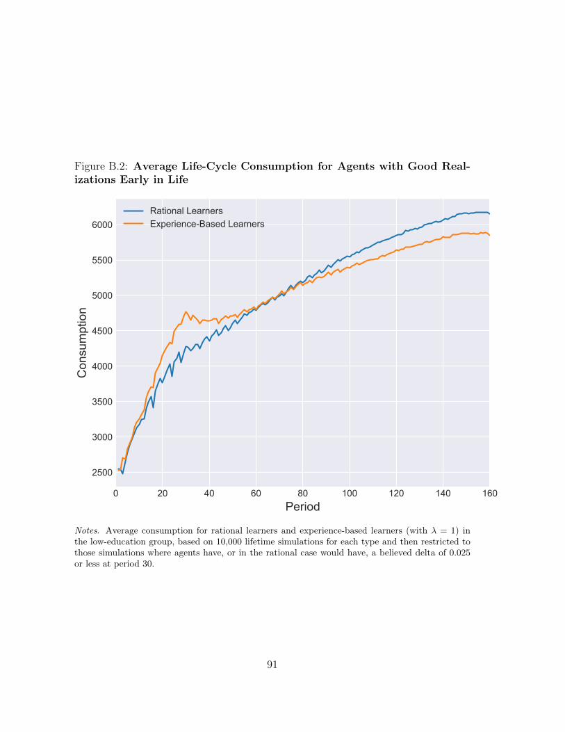
Figure B.2: Average Life-Cycle Consumption for Agents with Good Real-izations Early in Life

Notes. Average consumption for rational learners and experience-based learners (with � = 1) inthe low-education group, based on 10,000 lifetime simulations for each type and then restricted tothose simulations where agents have, or in the rational case would have, a believed delta of 0.025or less at period 30.

91

Figure B.3: Average Life-Cycle Consumption Patterns for Agents with BadRealizations Early in Life

Notes. Average consumption for rational learners and experience-based learners (with � = 1) inthe low-education group, based on 10,000 lifetime simulations for each type and then restricted tothose simulations where agents have, or in the rational case would have, a believed delta of 0.1 orgreater at period 30.

92

Figure B.1 depicts the resulting average consumption trends of rational and

experience-based learners during their working years, which are the years used in

the regressions. The graph hints at a pattern that, early in life, experience-based

learners underestimate the probability of job destruction, spend more, and must then

save more towards the end of their working life.

Figure B.2 provides an amplified illustration of the di↵erences. In this figure,

we only consider the subset of experience-based learners in the simulation who, at

period 30, have a believed delta of 0.025 or less and, in the rational case, the subset

of agents who would have a believed delta of 0.025 or less at period 30 if they were

experience-based learners. Since the true probability of job destruction is 0.049, these

agents were “lucky” early in life. For these consumers, the trend of over-consumption

among experienced based learners in the early periods is much more pronounced.

Figure B.3 illustrates the opposite scenario. Here, we only consider the subset of

experience-based learners in the simulation who, at period 30, have a believed delta

of 0.1 or greater, as well as the corresponding rational agents. In light of the true

probability of job destruction of 0.049, these agents have had bad luck early in life.

This “unlucky” group of experience-based learners has a markedly di↵erent savings

pattern. They consistently consume less than their rational counterparts for almost

their entire lives. Moreover, the illustration hints at an additional prediction, wealth

build-up due to excess frugality .

93