K: a Rewrite-based Framework for Modular Language

Design, Semantics, Analysis and Implementation

—Version 2—

Grigore Rosu∗

Department of Computer Science,University of Illinois at Urbana-Champaign

Abstract

K is an algebraic framework for defining programming languages. It consists of a techniqueand of a specialized and highly optimized notation. The K-technique, which can be best ex-plained in terms of rewriting modulo equations or in terms of rewriting logic, is based on afirst-order representation of continuations with intensive use of matching modulo associativity,commutativity and identity. The K-notation consists of a series of high-level conventions thatmake the programming language definitions intuitive, easy to understand, to read and to teach,compact, modular and scalable. One important notational convention is based on context trans-formers, allowing one to automatically synthesize concrete rewrite rules from more abstractdefinitions once the concrete structure of the state is provided, by “completing” the contextsin which the rules should apply. The K framework is introduced by defining FUN, a concurrenthigher-order programming language with parametric exceptions. A rewrite logic definition of aprogramming language can be executed on rewrite engines, thus providing an interpreter for thelanguage for free, but also gives an initial model semantics, amenable to formal analysis suchas model checking and inductive theorem proving. Rewrite logic definitions in K can lead toautomatic, correct-by-construction generation of interpreters, compilers and analysis tools.

Note to readers: The material presented in this report serves as a basis for programminglanguage design and semantics classes and for several research projects. This report aims at giv-ing a global snapshot of this rapidly evolving domain. Consequently, this work will be publishedon a version by version basis, each including and improving the previous ones, probably over aperiod of several years. This version already contains the desired structure of the final version,but not all sections are filled in yet. In this first version I put more emphasis on introducing theK framework and on how to use it. Here I focus less on related work, inductive verification andimplementation; these will be approached in next versions of this work. My plan is to eventuallytransform this material into a book, so your suggestions and criticisms are welcome.

∗Supported by joint NSF grants CCF-0234524, CCF-0448501, and CNS-0509321.

1

Contents

1 Introduction 4

2 An Overview of K 8

3 Rewriting Logic 253.1 Equational Logics . . . . . . . . . . . . . . . . . . . . . . . . . . . . . . . . . . . . . . 253.2 Term Rewriting . . . . . . . . . . . . . . . . . . . . . . . . . . . . . . . . . . . . . . . 253.3 Rewriting Logic . . . . . . . . . . . . . . . . . . . . . . . . . . . . . . . . . . . . . . . 27

4 Related Work 334.1 Structural Operational Semantics (SOS) . . . . . . . . . . . . . . . . . . . . . . . . . 334.2 Modular Structural Operational Semantics (MSOS) . . . . . . . . . . . . . . . . . . 334.3 Reduction Semantics and Evaluation Contexts . . . . . . . . . . . . . . . . . . . . . 334.4 Rewriting Logic Semantics . . . . . . . . . . . . . . . . . . . . . . . . . . . . . . . . . 344.5 Abstract State Machines . . . . . . . . . . . . . . . . . . . . . . . . . . . . . . . . . . 344.6 Logic Programming Semantics . . . . . . . . . . . . . . . . . . . . . . . . . . . . . . 344.7 Monads . . . . . . . . . . . . . . . . . . . . . . . . . . . . . . . . . . . . . . . . . . . 344.8 SECD Machine . . . . . . . . . . . . . . . . . . . . . . . . . . . . . . . . . . . . . . . 34

5 The K-Notation 355.1 Matching Modulo Associativity, Commutativity, Identity . . . . . . . . . . . . . . . . 355.2 Sort Inference . . . . . . . . . . . . . . . . . . . . . . . . . . . . . . . . . . . . . . . . 365.3 Underscore Variables . . . . . . . . . . . . . . . . . . . . . . . . . . . . . . . . . . . . 375.4 Tuples . . . . . . . . . . . . . . . . . . . . . . . . . . . . . . . . . . . . . . . . . . . . 385.5 Contextual Notation for Equations and Rules . . . . . . . . . . . . . . . . . . . . . . 385.6 Structural, Computational and Non-Deterministic Contextual Rules . . . . . . . . . 405.7 Matching Prefixes, Suffixes and Fragments . . . . . . . . . . . . . . . . . . . . . . . . 425.8 Structural Operations . . . . . . . . . . . . . . . . . . . . . . . . . . . . . . . . . . . 445.9 Context Transformers . . . . . . . . . . . . . . . . . . . . . . . . . . . . . . . . . . . 47

6 The K-Technique: Defining the FUN Language 516.1 Syntax . . . . . . . . . . . . . . . . . . . . . . . . . . . . . . . . . . . . . . . . . . . . 516.2 State Infrastructure . . . . . . . . . . . . . . . . . . . . . . . . . . . . . . . . . . . . 536.3 Continuations . . . . . . . . . . . . . . . . . . . . . . . . . . . . . . . . . . . . . . . . 536.4 Helping Operators . . . . . . . . . . . . . . . . . . . . . . . . . . . . . . . . . . . . . 556.5 Defining FUN’s Features . . . . . . . . . . . . . . . . . . . . . . . . . . . . . . . . . . 58

6.5.1 Global Operations: Eval and Result . . . . . . . . . . . . . . . . . . . . . . . 586.5.2 Syntactic Subcategories: Variables, Bool, Int, Real . . . . . . . . . . . . . . . 596.5.3 Operator Attributes . . . . . . . . . . . . . . . . . . . . . . . . . . . . . . . . 606.5.4 The Conditional . . . . . . . . . . . . . . . . . . . . . . . . . . . . . . . . . . 636.5.5 Functions . . . . . . . . . . . . . . . . . . . . . . . . . . . . . . . . . . . . . . 646.5.6 Let and Letrec . . . . . . . . . . . . . . . . . . . . . . . . . . . . . . . . . . . 656.5.7 Sequential Composition and Assignment . . . . . . . . . . . . . . . . . . . . . 656.5.8 Lists . . . . . . . . . . . . . . . . . . . . . . . . . . . . . . . . . . . . . . . . . 66

2

6.5.9 Input/Output: Read and Print . . . . . . . . . . . . . . . . . . . . . . . . . . 666.5.10 Parametric Exceptions . . . . . . . . . . . . . . . . . . . . . . . . . . . . . . . 676.5.11 Loops with Break and Continue . . . . . . . . . . . . . . . . . . . . . . . . . 67

7 Defining KOOL: An Object-Oriented Language 69

8 On Modular Language Design 708.1 Variations of a Simple Language . . . . . . . . . . . . . . . . . . . . . . . . . . . . . 708.2 Adding Call/cc to FUN . . . . . . . . . . . . . . . . . . . . . . . . . . . . . . . . . . 788.3 Adding Concurrency to FUN . . . . . . . . . . . . . . . . . . . . . . . . . . . . . . . 798.4 Translating MSOS to K . . . . . . . . . . . . . . . . . . . . . . . . . . . . . . . . . . 828.5 Discussion on Modularity . . . . . . . . . . . . . . . . . . . . . . . . . . . . . . . . . 83

8.5.1 Changes in State Infrastructure . . . . . . . . . . . . . . . . . . . . . . . . . . 838.5.2 Control-Intensive Language Constructs . . . . . . . . . . . . . . . . . . . . . 848.5.3 On Orthogonality of Language Features . . . . . . . . . . . . . . . . . . . . . 85

9 On Language Semantics 899.1 Initial Algebra Semantics Revisited . . . . . . . . . . . . . . . . . . . . . . . . . . . . 899.2 Initial Model Semantics in Rewriting Logic . . . . . . . . . . . . . . . . . . . . . . . 89

10 On Formal Analysis 9010.1 Type Checking . . . . . . . . . . . . . . . . . . . . . . . . . . . . . . . . . . . . . . . 9010.2 Type Inference . . . . . . . . . . . . . . . . . . . . . . . . . . . . . . . . . . . . . . . 10310.3 Type Preservation and Progress . . . . . . . . . . . . . . . . . . . . . . . . . . . . . . 12010.4 Concurrency Analysis . . . . . . . . . . . . . . . . . . . . . . . . . . . . . . . . . . . 12010.5 Model Checking . . . . . . . . . . . . . . . . . . . . . . . . . . . . . . . . . . . . . . . 120

11 On Implementation 121

12 Other Applications 122

13 Conclusion 123

A A Simple Rewrite Logic Theory in Maude 126

B Dining Philosophers in Maude 129

C Defining Lists and Sets in Maude 130

D Definition of Sequential λK in Maude 131

E Definition of Concurrent λK in Maude 136

F Definition of Sequential FUN in Maude 142

G Definition of Full FUN in Maude 151

3

1 Introduction

Appropriate frameworks for design and analysis of programming languages can not only help inunderstanding and teaching existing programming languages and paradigms, but can significantlyfacilitate our efforts and stimulate our desire to define and experiment with novel programminglanguages and programming language features, as well as programming paradigms or combinationsof paradigms. But what makes a programming language definitional framework appropriate? Webelieve that an ideal such framework should satisfy at least some core requirements; the followingare a few requirements that guided us in our quest for such a language definitional framework:

1. It should be generic, that is, not tied to any particular programming language or paradigm.For example, a framework enforcing object or thread communication via explicit send andreceive messages may require artificial encodings of languages that opt for a different com-munication approach, while a framework enforcing static typing of programs in the definedlanguage may be inconvenient for defining dynamically typed or untyped languages. In gen-eral, a framework providing and enforcing particular ways to define certain types of languagefeatures would lack genericity. Within an ideal framework, one can and should develop andadopt methodologies for defining certain types of languages or language features, but theseshould not be enforced. This genericity requirement is derived from the observation thattoday’s programming languages are so diverse and based on orthogonal, sometimes even con-flicting paradigms, that, regardless of how much we believe in the superiority of a particularlanguage paradigm, be it object-oriented, functional or logical, a commitment to any existingparadigm would significantly diminish the strengths of a language definitional framework.

2. It should be semantics-based, that is, based on formal definitions of languages rather thanon ad-hoc implementations of interpreters/compilers or program analysis tools. Semanticsis crucial to such an ideal definitional framework because, without a formal semantics ofa language, the problems of program analysis and interpreter or compiler correctness aremeaningless. One could use ad-hoc implementations to find errors in programs or compilers,but never to prove their correctness. Ideally, we would like to have one definition of a languageto serve all purposes, including parsing, interpretation, compilation, as well as formal analysisand verification of programs, such as static analysis, theorem proving and model checking.Having to annotate or slightly change/augment a language definition for certain purposes isacceptable and unavoidable; for example, certain domain-specific analyses may need domaininformation which is not present in the language definition; or, to more effectively model-checka concurrent program, one may impose abstractions that cannot be inferred automaticallyfrom the formal semantics of the language. However, having to develop an entirely newlanguage definition for each purpose should be unacceptable in an ideal definitional framework.

3. It should be executable. There is not much one can do about the correctness of a definition,except to accumulate confidence in it. In the case of a programming language, one canaccumulate confidence by proving desired properties of the language (but how many, when tostop?), or by proving equivalence to other formal definitions of the same language if they exist(but what if these definitions all have the same error?), or most practical of all, by having thepossibility to execute programs directly using the semantic definition of the language. In ourexperience, executing hundreds of programs exercising various features of a language helpsto not only find and fix errors in that language definition, but also stimulates the desire to

4

experiment with new features. A computational logic framework with efficient executabilityand a spectrum of meta-tools can serve as a basis to define executable formal semantics oflanguages, and also as a basis to develop generic formal analysis techniques and tools.

4. It should be able to naturally support concurrency. Due to the strong trend in parallelizingcomputing architectures for increased performance, probably most future programming lan-guages will be concurrent. To properly define and reason about concurrent languages, thesemantics of the underlying definitional framework should be inherently concurrent, ratherthan artificially graft support for concurrency on an essentially sequential paradigm, for ex-ample, by defining or simulating a process/thread scheduler. A semantics for true concurrencywould be preferred to one based on interleavings, because executions of concurrent programson parallel architectures are not interleaved.

5. It should be modular, to facilitate reuse of language features. In this context, modularityof a programming language definitional framework means more than just allowing groupinglanguage feature definitions in modules. What it means is the ability to add or removelanguage features without having to modify any definitions of other, unrelated features. Forexample, if one adds parametric exceptions to one’s language, then one should just includethe corresponding module and change no other definition of any other language feature. Ina modular framework, one can therefore define languages by adding features in a “plug-and-play” manner. A typical structural operational semantics (SOS) [22] definition of a languagelacks modularity because one needs to “update” all the SOS rules whenever the structure ofthe state, or configuration, changes (like in the case of adding support for exceptions).

6. It should allow one to define any desired level of computation granularity, to capture the var-ious degrees of abstraction of computation encountered in different programming languages.For example, some languages provide references as first class value citizens (e.g., C and C++);in order to get the value v that a reference variable x points to, one wants to perform twosemantic steps in such languages: first get the value l of x, which is a location, and then readthe value v at location l. However, other languages (e.g., Java) prefer not to make referencesvisible to programmers, but only to use them internally as an efficient means to refer tocomplex data-structures; in such languages, one thinks of grabbing the (value stored in a)data-structure in one semantic step, because its location is not visible. An ideal frameworkshould allow one to flexibly define any of these computation granularities. Another examplewould be the definition of functions with multiple arguments: an ideal framework should notenforce one to eliminate multiple arguments by currying; from a programming language designperspective, the fact that the underlying framework supports only one-argument functionsor abstractions is regarded as a limitation of the framework. Other examples are mentionedlater in the paper. Having the possibility to define different computation granularities fordifferent languages gives a language designer several important benefits: better understand-ing of the language by not having to bother with low level implementation-like or “encoding”details, more freedom in how to implement the language, more appropriate abstraction ofthe language for formal analysis of programs, such as theorem proving and model checking,etc. From a computation granularity perspective, an extreme worst case of a definitionalframework would provide a fixed computation granularity for all programming languages, forexample one based on encodings of language features in λ-calculus or on Turing machines.

5

There are additional desirable, yet more subjective and thus harder to quantify, requirementsof an ideal language definitional framework, including: it should be simple, easy to understand andteach; it should have good data representation capabilities; it should scale well, to apply to arbi-trarily large languages; it should allow proofs of theorems about programming languages that areeasy to comprehend; etc. The six requirements above are nevertheless ambitious. Moreover, thereare subtle tensions among them, making it hard to find an ideal language definitional framework.Some proponents of existing language definitional frameworks may argue that their favorite frame-work has these properties; however, a careful analysis of existing language definitional frameworksreveals that they actually fail to satisfy some, sometimes most, of these ideal features (we discussseveral such frameworks and their limitations in Section 4). Others may argue that their favoriteframework has some of the properties above, the “important ones”, declaring the other propertieseither “not interesting” or “something else”. For example, one may say that what is important inone’s framework is to get a dynamic semantics of a language, but its (model-theoretical) algebraicdenotational semantics, proving properties about programs, model checking, etc., are “somethingelse” and therefore are allowed to need a different “encoding” of the language. Our position is thatan ideal language definitional framework should not compromise any of the six requirements above.

Following up recent work in rewriting logic semantics [19, 18], in this paper we argue thatrewriting logic [17] can be a reasonable starting point towards the development of such an idealframework. We call it a “starting point” because we believe that without appropriate language-specific front-ends (notations, conventions, etc.) and without appropriate definitional techniques,rewriting logic is simply too general, like the machine code of a processor or a Turing machine ora λ-calculus. In a nutshell, one can think of rewriting logic as a framework that gives completesemantics (that is, models that make the expected rewrite relation, or “deduction”, complete) to theotherwise usual and standard term rewriting modulo equations. If one is specifically not interestedin the model-theoretical semantic dimension of the proposed framework, but only in its operational(including proof theoretical, model checking and, in general, formal verification) aspects, then onecan safely think of it as a framework to define programming languages as standard term rewritesystems modulo equations. The semantic counterpart is achieved at no additional cost (neitherconceptual nor notational), by just regarding rewrite systems as rewrite logic specifications.

A rewrite logic theory consists of a set of uninterpreted operations constrained equationally,together with a set of rewrite rules meant to define the concurrent evolution of the defined system.The distinction between equations and rewrite rules is only semantic. With few exceptions, theyare both executed as rewrite rules l → r by rewrite engines, following the simple, uniform andparallelizable match-and-apply principle of term rewriting: find a subterm matching l, say with asubstitution θ, then replace it by θ(r). Therefore, if one is interested in just a dynamic semanticsof a language, then, with few exceptions, one needs to make no distinction between equations andrewrite rules; the exceptions are some special equations, such as associativity and commutativity,enabling specialized algorithms in rewrite engines, which are used for non-computational purposes,namely for keeping structures, such as states, in convenient canonical forms.

Rewriting logic admits an initial model semantics, where equations form equivalence classes onterms and rewrite rules define transitions between such equivalence classes. Operationally, rewriterules can be applied concurrently, thus making rewrite logic a very simple, generic and universalframework for concurrency; indeed, many other theoretical frameworks for concurrency, includingπ-calculus, process algebra, actors, etc., have been seamlessly defined in rewriting logic [16]. Inour context of programming languages, a language definition is a rewrite logic theory in which (at

6

least) the concurrent features of the language are defined using rewrite rules. A program togetherwith its initial state are given as an uninterpreted term, whose denotation in the initial model is itscorresponding transition system. Depending on the desired type of analysis, one can, using existingtool support, generate anywhere from one path in that transition system (e.g., when “executing”the program) to all paths (e.g., for model checking).

One must, nevertheless, treat the simplicity and generality of rewriting logic with caution;“general” and “universal” need not necessarily mean “better” or “easier to use”, for the samereason that machine code is not better or easier to use than higher level programming languagesthat translate into it. In our context of defining programming languages in rewriting logic, theright questions to ask are whether rewriting logic provides a natural framework for this task or not,and whether we get any benefit from using it. In spite of its simplicity and generality, rewritinglogic does not give us any immediate recipe for how to define languages as rewrite logic theories.Appropriate definitional techniques and methodologies are necessary in order to make rewriting logican effective computational framework for programming language definition and formal analysis.

In this paper we propose K, a domain-specific language front-end to rewriting logic that al-lows for compact, modular, executable, expressive and easy to understand and change semanticdefinitions of programming languages, concurrent or not. K could be explained and presented or-thogonally to rewriting logic, as a standalone language definitional framework (same as, e.g., SOSor reduction semantics), but we prefer to regard it as a language-specific front-end to rewrite logicto reflect from the very beginning the fact that it inherits all the good properties and techniquesof rewriting logic, a well established formalism with many uses and powerful tool support.

As discussed in [19, 18, 4] and in Section 4 of this paper, other definitional frameworks, suchas SOS [22], MSOS [21] and reduction semantics [8], can also be easily translated into rewritinglogic. More precisely, for a particular language formalized using any of these formalisms, say F, onecan devise a rewrite logic specification, say RF, which is precisely the intended original languagedefinition F, not an artificial encoding of it ; in other words, there is a one-to-one correspondencebetween derivations using F and rewrite logic derivations using RF, obviously modulo a differentbut minor and ultimately irrelevant syntactic notation. This way, RF has all the properties, goodor bad, of F. However, in order to achieve such a bijective correspondence and thus the faithfultranslation of F into rewriting logic, one typically has to significantly restrain the strength ofrewriting logic, reducing it to a limited computational framework, just like F. For example, thefaithful translation of SOS definitions requires one conditional rewrite rule per SOS rule, but theresulting rewrite logic definition can apply rewrites only at the top, just like SOS, thus enforcingalways an interleaving semantics for concurrent languages, just like SOS. Therefore, the fact thatthese formalisms translate into rewriting logic does not necessarily mean that they inherit allthe good properties of rewriting logic. However, K extends rewriting logic with features that aremeaningful for programming language formal definitions but which can be translated automaticallyback into rewriting logic, so K is rewriting logic.

7

2 An Overview of K

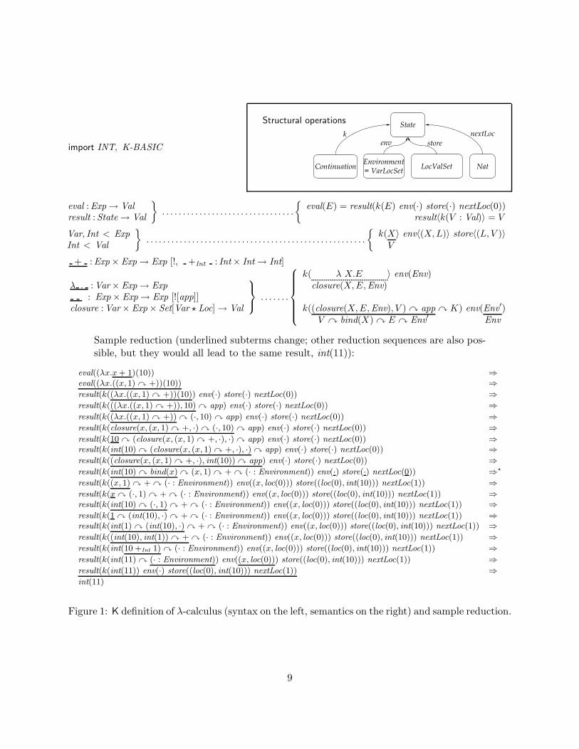
Figure 1 shows a definition in K of untyped λ-calculus with builtin integers, together with a samplereduction of simple program. Since a more complex language is discussed shortly, we refrainfrom commenting this definition here (though the reader may partly anticipate how K works bytrying to decipher it). We only enphasize that the language definition in Figure 1 is formal (itis an equational theory with initial model semantics) and executable. The five rules on the rightare for initialization of the evaluation process, for collecting and outputing the final result, forvariable lookup, for function evaluation to closures and for function invocation. Any definitionalor implementation framework should explicitly or implicitly provide these operations. From alanguage design, semantics and implementation perspective, the fact that one can define λ-calculuseasily in one’s framework should mean close to nothing: any framework worth mentioning shouldbe capable of doing that. The sole reason for which we depict the definition of λ-calculus here isto show the reader how a familiar language looks when defined in K. Section ?? shows how K canmodularly define the series of variations of this simple language suggested in [29].

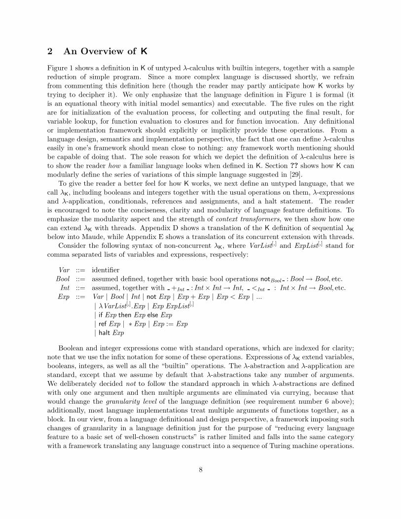
To give the reader a better feel for how K works, we next define an untyped language, that wecall λK, including booleans and integers together with the usual operations on them, λ-expressionsand λ-application, conditionals, references and assignments, and a halt statement. The readeris encouraged to note the conciseness, clarity and modularity of language feature definitions. Toemphasize the modularity aspect and the strength of context transformers, we then show how onecan extend λK with threads. Appendix D shows a translation of the K definition of sequential λK

below into Maude, while Appendix E shows a translation of its concurrent extension with threads.Consider the following syntax of non-concurrent λK, where VarList[,] and ExpList[,] stand for

comma separated lists of variables and expressions, respectively:

Var ::= identifierBool ::= assumed defined, together with basic bool operations notBool :Bool→ Bool, etc.Int ::= assumed, together with +Int : Int× Int→ Int, <Int : Int× Int→ Bool, etc.

Exp ::= Var | Bool | Int | not Exp | Exp + Exp | Exp < Exp | ...| λVarList[,].Exp | Exp ExpList[,]

| if Exp then Exp else Exp| ref Exp | ∗ Exp | Exp := Exp| halt Exp

Boolean and integer expressions come with standard operations, which are indexed for clarity;note that we use the infix notation for some of these operations. Expressions of λK extend variables,booleans, integers, as well as all the “builtin” operations. The λ-abstraction and λ-application arestandard, except that we assume by default that λ-abstractions take any number of arguments.We deliberately decided not to follow the standard approach in which λ-abstractions are definedwith only one argument and then multiple arguments are eliminated via currying, because thatwould change the granularity level of the language definition (see requirement number 6 above);additionally, most language implementations treat multiple arguments of functions together, as ablock. In our view, from a language definitional and design perspective, a framework imposing suchchanges of granularity in a language definition just for the purpose of “reducing every languagefeature to a basic set of well-chosen constructs” is rather limited and falls into the same categorywith a framework translating any language construct into a sequence of Turing machine operations.

8

import INT, K-BASIC

Structural operations

Continuation

k

Environment= VarLocSet Nat

env

LocValSet

State

storenextLoc

eval :Exp→ Valresult :State→ Val

}. . . . . . . . . . . . . . . . . . . . . . . . . . . . . . . .

{eval(E) = result(k(E) env(·) store(·) nextLoc(0))

result〈k(V : Val)〉 = V

Var, Int < ExpInt < Val

}. . . . . . . . . . . . . . . . . . . . . . . . . . . . . . . . . . . . . . . . . . . . . . . . . . . . .

{k(X

V〉 env〈(X, L)〉 store〈(L, V )〉

+ :Exp× Exp→ Exp [!, +Int : Int× Int→ Int]

λ . :Var× Exp→ Exp: Exp× Exp→ Exp [![app]]

closure :Var× Exp× Set[Var � Loc]→ Val

⎫⎬⎭ . . . . . . .

⎧⎪⎪⎪⎪⎨⎪⎪⎪⎪⎩

k( λ X.Eclosure(X, E,Env)

〉 env(Env)

k((closure(X, E,Env), V ) � appV � bind(X) � E � Env′

� K) env(Env′

Env)

Sample reduction (underlined subterms change; other reduction sequences are also pos-sible, but they would all lead to the same result, int(11)):

eval((λx.x + 1)(10)) ⇒eval((λx.((x,1) � +))(10)) ⇒result(k((λx.((x, 1) � +))(10)) env(·) store(·) nextLoc(0)) ⇒result(k(((λx.((x, 1) � +)), 10) � app) env(·) store(·) nextLoc(0)) ⇒result(k((λx.((x, 1) � +)) � (·, 10) � app) env(·) store(·) nextLoc(0)) ⇒result(k(closure(x, (x, 1) � +, ·) � (·, 10) � app) env(·) store(·) nextLoc(0)) ⇒result(k(10 � (closure(x, (x, 1) � +, ·), ·) � app) env(·) store(·) nextLoc(0)) ⇒result(k(int(10) � (closure(x, (x, 1) � +, ·), ·) � app) env(·) store(·) nextLoc(0)) ⇒result(k((closure(x, (x, 1) � +, ·), int(10)) � app) env(·) store(·) nextLoc(0)) ⇒result(k(int(10) � bind(x) � (x, 1) � + � (· : Environment)) env(·) store(·) nextLoc(0)) ⇒�

result(k((x, 1) � + � (· : Environment)) env((x, loc(0))) store((loc(0), int(10))) nextLoc(1)) ⇒result(k(x � (·, 1) � + � (· : Environment)) env((x, loc(0))) store((loc(0), int(10))) nextLoc(1)) ⇒result(k(int(10) � (·, 1) � + � (· : Environment)) env((x, loc(0))) store((loc(0), int(10))) nextLoc(1)) ⇒result(k(1 � (int(10), ·) � + � (· : Environment)) env((x, loc(0))) store((loc(0), int(10))) nextLoc(1)) ⇒result(k(int(1) � (int(10), ·) � + � (· : Environment)) env((x, loc(0))) store((loc(0), int(10))) nextLoc(1)) ⇒result(k((int(10), int(1)) � + � (· : Environment)) env((x, loc(0))) store((loc(0), int(10))) nextLoc(1)) ⇒result(k(int(10 +Int 1) � (· : Environment)) env((x, loc(0))) store((loc(0), int(10))) nextLoc(1)) ⇒result(k(int(11) � (· : Environment)) env((x, loc(0))) store((loc(0), int(10))) nextLoc(1)) ⇒result(k(int(11)) env(·) store((loc(0), int(10))) nextLoc(1)) ⇒int(11)

Figure 1: K definition of λ-calculus (syntax on the left, semantics on the right) and sample reduction.

9

We will later see that rewriting logic, and implicitly K, allow us to tune the granularity of com-putation also via equational abstraction: if certain rules are not intended to generate computationsteps in the semantics of a language, then we make them equations; the more equations versus rulesin a language definition, the fewer computational steps (and the larger the equivalence classes ofterms/expressions/programs in the initial model of that language’s definition).

For simplicity, we here assume a call-by-value evaluation strategy in λK; the other evaluationstrategies for languages defined in K present no difficulty and are taught on a regular basis tograduate and undergraduate students [24].

NEXT-VERSION: add different parameter passing styles and eventually a LAZY-FUN

. The conditional expression expects its first argument to evaluate to a boolean and then, dependingon its truth value, evaluates to either its second or its third expression argument; note that forthe conditional we used the “mix-fix” syntactic notation, rather then a prefix one. The expressionref E evaluates E to some value, stores it at some location or reference, and then returns thatreference as a result of its evaluation; therefore, in λK we (semantically) assume that referencesare first-class values in the language even though the programmer cannot use them in programsexplicitly, since the syntax of λK does not define references (it actually does not define values,either). The expression ∗ R, called dereferencing of R, evaluates R to a reference and then returnsthe value stored at that reference. The expression R := E, called assignment, first evaluates R toan (existing) reference r and E to a value v, and then writes v at r; the value v is also the result ofthe evaluation of the assignment. Finally, the expression halt E evaluates E to some value v andthen aborts the computation and returns v as a result.

We next define the usual let bindings and sequential composition as syntactic sugar over λK:

• let X = E in E′ is (λX.E′)E,

• let F (X) = E in E′ is (λF.E′)(λX.E),

• let F (X,Y ) = E in E′ is (λF.E′)(λX, Y.E), etc., and

• E;E′ is (λD.E′)E, where D is a fresh “dummy” variable; thus, E is first evaluated (recallthat we assume call-by-value parameter passing), its value bound to D and discarded, andthen E′ is evaluated.

If these constructs were intended to be part of the language, then these definitions are clearlynot suitable from a computational granularity point of view, because they change the intendedgranularity of these language constructs. In Section 6, we show how statements like these andmany others can be defined directly (without translating them to other constructs), in the contextof the more complex FUN language. For now, we can regard them as “notational conventions” forthe more complex, equivalent expressions. With these conventions, the following is a λK expressionthat calculates factorial of n (here, n is regarded as a “macro”; also, note that this code cannot beused as part of a function to return the result of the factorial, because halt terminates the program— one could do it if one defines parametric exceptions as we do later in the paper, and then throwan exception instead of halt):

let r = ref nin let g(m,h) = if m > 1 then (r := (∗r) ∗m; h(m− 1, h)) else halt (∗r)

in g(n − 1, g)

10

While λK is clearly a very simple toy language, we believe that it contains some canonicalfeatures that any ideal language definitional framework should be able to support naturally. Indeed,if a framework cannot define λ-expressions naturally than that framework is inappropriate to definemost functional languages and most likely many other non-trivial languages. The conditionalstatement has been chosen for two reasons: first, most languages have conditional statements asa means to allow various control flows in programs, and, second, conditionals have an interestingevaluation strategy, namely strict in the first argument and lazy in the second and third; therefore,a naive use of a purely “lazy” or a purely “strict” definitional framework may lead to inconvenientencodings of conditionals. References are either directly or indirectly part of several mainstreamlanguages, so they must present no difficulty in any language definitional framework. Finally, haltis one of the simplest control-intensive language constructs; if a language definitional frameworkcannot define halt naturally, then it most likely cannot define any control-intensive statements,including break and continue of loops, exceptions, and call/cc.

On the other hand, if a language definitional framework can define the λK language aboveeasily, then it most likely can define many other programming language constructs of interest. Ourpurpose for introducing λK here is not to highlight specific features that languages could or shouldhave, but instead to highlight that a language definitional framework should be flexible enough tosupport a rapid, yet formal, investigation of language features, lowering the boundary between newideas and executable systems for trying these ideas. An important language feature that we havedeliberately not added yet to λK is concurrency; that is because many existing frameworks weredesigned for sequential languages and one may therefore argue that a comparison of those with Kon a concurrent language would not be fair. However, we will add threads to λK shortly and showhow they can be given a semantics in K in a straightforward manner. Concurrent λK shows mostof the subtleties of our framework.

The language definitional framework K consists of two important components:

• The K-notation, which can be regarded as a programming language specific front-end torewriting logic, allows users to focus fully on the actual semantics of language features, ratherthan on distracting details or artifacts of rewriting logic, such as complete sort and operationdeclarations even though these can be trivially inferred from context, or adding concep-tually unrelated state context just for the purpose of well formedness of the rewrite logictheory defining the feature under consideration, even though some partially well formed the-ory could be completed in a unique way entirely automatically. Besides clarity of definitionsof programming language concepts, an additional driving force underlying the design of theK-notation was compactness of definitions, which is closely related to modularity of program-ming language definitions: any unnecessary piece of information (including sort and operationdeclarations) that we mention in a language feature definition may work against us when usingthat feature in a different context.

• The K-technique is a technique to define programming languages algebraically, based on afirst-order representation of continuations. Recall that a continuation encodes the remainingcomputation [23, 26]. Specifically, a continuation is a structure that comes with an implicitor explicit evaluation mechanism such that, when passed a value (thought of as the valueof some local computation), it “knows” how to finish the entire computation. Since theyprovide convenient, explicit representations of computation flows as ordinary data, contin-uations are useful especially in the context of defining control-intensive statements, such as

11

exceptions. Note, though, that continuations typically encode only the computation steps,not the store; therefore, one still needs to refer to external data during their evaluation. Tra-ditionally, continuations are encoded as higher-order functions, which is very convenient inthe presence of higher-order languages, because one uses the implicit evaluation mechanism ofthese languages to evaluate continuations as well. Our K-technique is, however, not based onencodings of continuations as higher-order functions. That is partly because our underlyingalgebraic infrastructure is not higher-order (though, as we are showing here, one can definehigher-order functions); we can more easily give a different encoding of continuations, namelyone based on lists of tasks, together with an explicit stack-like evaluation mechanism.

We introduce the K-notation and the K-technique together as part of our framework K, becausewe think that they fit very well together. However, one can nevertheless use them independently;for example, one can use the K-notation in algebraic specification or rewrite-based applicationsnot necessarily related to programming languages, and one can employ the K-technique to defineprogramming languages in any reduction-based framework, ignoring entirely the proposed notation.An ideal name for our framework would have been “C”, since our technique is based on continuationsand our trickiest notational convention is that for context transformers, but this letter is alreadyassociated to a programming language. To avoid confusion we use the letter “K” instead.

Figure 2 shows the complete definition of λK in K, including both its syntax and its semantics.The imported modules BOOL, INT and K-BASIC contain basic definitions of booleans, of integernumbers and of infrastructure operations that tend to be used by most language definitions. We willdiscuss these later, together with other technical details underlying the K framework; we here onlymention that these modules can be either defined in the same style as other language features, thatis, as rewrite logic theories using the K framework, or defined or even implemented as builtins. Herewe only present the major characteristics and intuitions underlying the K definitional framework. Itis fair to say upfront that we have not implemented either a parser of K or an automatic translatorof K into rewriting logic or other formalisms yet; currently, we are using it as an alternative toSOS or reduction semantics to define languages, which can be then straightforwardly translatedinto rewrite logic definitions (note that SOS or reduction semantics language definitions cannotbe “straightforwardly” translated into rewriting logic; these need to follow generic and systematictransformation steps resulting in rather constrained and unnatural rewrite logic theories – seeSection 4). However, K was designed to be implementable as is; therefore, even though we do nothave machine support for it yet, we think of the subsequent definitions, in particular the one of λK

in Figure 2, as machine executable.The modules BOOL and INT come with sorts Bool, Int and Nat, where Nat is a subsort of Int.

The module K-BASIC comes with sorts Exp, Val and Loc, for expressions, values and locations,respectively; no subsort relations are assumed among these sorts, in particular the sort Val is nota subsort of Exp – indeed, values are not expressions in general (e.g., a closure is a value but notan expression). Locations also come with a constructor operation location : Nat → Loc and anoperation next : Loc → Loc, which gives the next available location; for simplicity, in this paperwe assume that next(location(N)) = location(N + 1), but one is free to define a garbage collectorreturning the next unoccupied location. One additional and very important sort that the moduleK-BASIC comes with is Continuation, which is a supersort of both Exp and Val (in fact, it is asupersort of lists of expressions and of lists of values), which is structured as a list (of “tasks”). Kis a modular framework, that is, language features can be added to or dropped from a languagewithout having to change any other unrelated features. However, for simplicity, we here refrain

12

import BOOL, INT, K-BASIC

Structural operations

Continuation

k

VarLocSet Nat

env

LocValSet

State

store nextLoc

eval : Exp→ Valresult : State→ Val

}. . . . . . . . . . . . . . . . . . . . . . . . . .

⎧⎪⎪⎪⎪⎨⎪⎪⎪⎪⎩

eval(E)result(k(E) env(·) store(·) nextLoc(0))

( 1)

result〈k(V )〉V

( 2)

Var, Bool, Int < ExpBool, Int < Val

}. . . . . . . . . . . . . . . . . . . . . . . . . . . . . . . .

{k(X

V

〉 env〈(X,L)〉 store〈(L, V )〉 ( 3)

not : Exp→ Exp [!, notBool : Bool → Bool ]+ :Exp× Exp→ Exp [!, +Int : Int× Int→ Int]< : Exp× Exp→ Exp [!, <Int : Int× Int→ Bool]

λ . :VarList× Exp→ Exp:Exp× ExpList→ Exp [![app]]

closure :VarList × Exp× VarLocSet→ Val

⎫⎬⎭ . .

⎧⎪⎪⎪⎪⎨⎪⎪⎪⎪⎩

k( λXl.E

closure(Xl,E,Env)〉 env(Env) ( 4)

k((closure(Xl,E,Env),V l)�appV l � bind(Xl) � E � Env′

〉 env(Env′

Env) ( 5)

if then else : Exp× Exp× Exp→ Exp [!(1)[if]]} . . . . . . . . . . . . . . .

⎧⎪⎪⎪⎪⎨⎪⎪⎪⎪⎩

bool (true) � if(E1, E2)E1

( 6)

bool (false) � if(E1, E2)E2

( 7)

Loc < Valref :Exp→ Exp [!]� :Exp→ Exp [!]:= :Exp× Exp→ Exp [!]

⎫⎪⎪⎬⎪⎪⎭

. . . . . . . . . . . . .

⎧⎪⎪⎪⎪⎪⎪⎪⎪⎪⎪⎨⎪⎪⎪⎪⎪⎪⎪⎪⎪⎪⎩

k(V � refloc(L)

〉 nextLoc( L

next(L)) store〈 ·

(L, V )〉 ( 8)

k(loc(L) � �

V

〉 store〈(L, V )〉 ( 9)

k((loc(L), V ) � :=V

〉 store〈(L,

V

)〉 (10)

halt :Exp→ Exp [!]}

. . . . . . . . . . . . . . . . . . . . . . . . . . . . . . . . . . . . . . . . . . . . . .{

k(V � halt �

·) (11)

Figure 2: Definition of Syntax and Semantics of λK in K

13

from defining modules and their corresponding module composition operations.A K language definition contains module imports, declarations of operations (which can be

structural, language constructs, or just ordinary), and declarations of contextual rules. For eachsort Sort, in K we implicitly assume corresponding sorts SortList and SortSet for lists and setsof sort Sort, respectively. By default, we use the (same) infix associative comma operation ,as a constructor for lists of any sort, and the infix associative and commutative operationas a constructor for sets of any sort. One important exception from the comma notation is thecontinuation construct, written � , which sequentializes evaluation tasks: e.g., the list (E,E′) �

+ � write(X) should read “first evaluate the expressions E and E′, then sum their values, thenwrite the result to X”; in module K-BASIC, the sort Continuation is declared as an alias for the sortContinuationItemList, where ContinuationItem is declared as a supersort of ExpList and ValList,and is typically extended with new constructs in a language definition (such as the “+” above).By convention, tuple sorts Sort1Sort2...Sortn and tuple operations ( , , ..., ) : Sort1 × Sort2 ×· · · Sortn → Sort1Sort2...Sortn are assumed tacitly, without declaring them explicitly, wheneverneeded. Also, some procedure will be assumed for sort inference for variables; this will relieveus from declaring obvious sorts and thus keep the formal programming language definitions moreinteresting and compact. By convention, variables start with a capital letter. If the sort inferenceof a variable is ambiguous, or simply for clarity reasons, one can manually sort, or annotate, anysubterm, using the notation t : Sort; in particular, t can be a variable. This manual sorting can beused by the sort inference procedure to both eliminate ambiguities and improve efficiency.

Structural operations, which we prefer to define graphically as a tree whose nodes are sorts andwhose edges are operation declarations, are those that give the structure of the state. When moreedges go into the same node, the target sort is automatically assumed a multiset sort, each of theincoming operations generating an element of that set. For example, the sort State in Figure 2is a set sort, while k (continuation), env (environment), store, and nextLoc (next location) cangenerate elements of State; these elements are also called state attributes. All the corresponding setoperation declarations and equations are added automatically. Structural operations will be usedin the process of context transformation of rules that will be explained shortly. The distinguishedcharacteristic of K is its contextual rule. A contextual rule consists of a term C, called the context,in which some subterms t1, ..., tn, which are underlined, are substituted by other terms t′1, ...,t′n, written underneath the lines. Contextual rules can be automatically translated into equationsor rewrite rules. Our motivation for contextual rules came from the observation that in manyrewriting logic definitions of programming languages, large terms tend to appear in the left handsides of rewrite rules only to create the context in which a small change should take place; the righthand sides of such rewrite rules consist mostly of repeating the left ones, thus making them hardto read and error prone.

When writing K definitions, for clarity we prefer to write the syntax on the left and the cor-responding semantics on the right. There will typically be one or at most two semantic rules persyntactic language construct. At this moment we do not make a distinction between declarations ofoperations intended to define the syntax of a language and the declarations of auxiliary operationsthat are necessary only to define the semantics; for the time being we assume that the distinctionis clear, but in the forthcoming implementation of K we will have designated operator annotationsfor this purpose. Tacitly, we tend to use sans serif font for the former and italic font for the latter.

In the definition of λK in Figure 2, the auxiliary operations eval and result are used to createthe appropriate state context and to extract the resulting value when the computation is finished,

14

respectively. Their definitions consist of trivial contextual rules: eval(E) creates the initial statewith E in the continuation, empty environment and store, and first free location 0, and thenwraps it with the operator result. The rules corresponding to various features of the language willeventually evaluate E to a value, which will reside as the only item in the continuation at the endof the computation. Then the rule corresponding to result will collapse everything to that value.

Note the use of the angle brackets “〈” and “〉” in the rule for result. These can be used wherevera list or a set is expected, to signify that there may be more elements to the left or to the rightof the enclosed term, respectively: “〈t〉” reads “the term t appears somewhere in the list or set”,“(t〉” reads “t appears as a prefix of the list or set”, and “〈t)” reads “t appears as a suffix of the listor set”; they are all equivalent in the case of sets, in which case we prefer the former. Intuitively,“〈” can be read “and so on to the left” and “〉” can be read “and so on to the right”. Therefore,the contextual rule of result says that if the term to reduce will ever consist of a result operatorwrapping a state that contains a continuation that contains a value V , then replace the entire termby V . The sort Val of V can be automatically inferred, because the result sort of result is Val.

We next say via subsort declarations that variables, booleans and integers are all expressions,and that booleans and integers are also values. K adds automatically an operation valuesort :Valuesort → Val for each sort Valuesort that is declared a subsort of Val. In our case, operationsbool : Bool→ Val and int : Int→ Val are added now, and another operation loc : Loc→ Val will beadded later, when the subsort declaration Loc < Val appears. Also, for those sorts Valuesort thatare subsorts of both Val and Exp, a contextual rule of the form

k( Evvaluesort(Ev)

〉

is automatically considered in K, saying that whenever an expression Ev of sort Valuesort (inferredfrom the fact that Ev appears as an argument of valuesort) appears at the top of the continua-tion, that is, if it is the next task to evaluate, then simply replace it by the corresponding value,valuesort(Ev). Rule (3) gives the semantics of variable lookup: if variable X is the next task inthe continuation (note the “〉” angle bracket matching the rest of the continuation), and if the pair(X,L) appears in the environment (here note both angle brackets), and if the pair (L, V ) appearsin the store, then just replace X by V at the top of the continuation; note also that the right sortsfor variables can be automatically inferred.

Let us next briefly discuss the operator attributes. The operations not, + , as well as theother operators extending the builtin operations, have two attributes, an exclamation mark “!”and the operations they extend. The exclamation mark, called strictness attribute, says that theoperation is strict in its arguments in the order they appear, that is, its arguments are evaluatedfirst (from left to right) and then the actual operation is applied. An exclamation mark attributecan take a list of numbers as optional argument and one optional attribute, like in the case of theconditional. These decorations of the strictness attribute can be fully and automatically translatedinto corresponding rules. We next discuss these.

If the exclamation mark attribute has a list of numbers argument, then it means that theoperation is declared strict in those arguments in the given order. Note that the missing argumentof a strictness attribute is just a syntactic sugar convenience; indeed, an operator with n argumentswhich is declared just “strict” using a plain “!” attribute, is entirely equivalent to one whoseattribute is “!(1 2 . . . n)”. When evaluating an operation declared using a strictness attribute,the arguments in which the operation was declared strict (i.e., the argument list of “!”) are first

15

scheduled for evaluation; the remaining arguments need to be “frozen” until the other argumentsare evaluated. If the exclamation mark attribute has an attribute, say att, then att will be used asa continuation item constructor to “wrap” the frozen arguments. Similarly, the lack of an attributeassociated to a strictness attribute corresponds to a default attribute, which by convention hasthe same name as the corresponding operation; to avoid confusion with underscore variables, wedrop all the underscores from the original language construct name when calculating the defaultname of the attribute of “!”. For example, an operation declared “ + :Exp× Exp→ Exp [!]” isautomatically desugared into “ + :Exp× Exp→ Exp [!(1 2)[+]]”.

Let us next discuss how K generates corresponding rules from strictness attributes. Supposethat we declare a strict operation, say op, whose strictness attribute has an attribute att. Then Kautomatically adds

(a) an auxiliary operation att to the signature, whose arguments (number, order and sorts) areprecisely the arguments of op in which op is not strict; the result sort of this auxiliaryoperation is ContinuationItem;

(b) a rule initiating the evaluation of the strict arguments in the specified order, followed by theother arguments “frozen”, i.e., wrapped, by the corresponding auxiliary operation att.

For example, in the case of λK’s conditional whose strictness attribute is “!(1)[if]”, an operation“if :Exp× Exp→ ContinuationItem is automatically added to the signature, together with a rule

if E then E1 else E2

E � if(E1, E2)

If the original operation is strict in all its arguments, like not, + and , then the auxiliaryoperation added has no arguments (it is a constant). For example, in the case of λK’s applicationwhose strictness attribute is “![app]”, an operation “app :→ ContinuationItem is added to thesignature, together with a rule

E El(E,El) � app

The “builtin” operations added as attributes to some language constructs, such as +Int : Int×Int → Int as an attribute of + :Exp × Exp → Exp, each corresponds to precisely one K-rulethat “calls” the builtin on the right arguments. This convention will be explained in detail later inthe paper; we here only show the two implicit rules corresponding to the attributes of the additionoperator in Figure 2:

E1 + E2

(E1, E2) � +

(int(I1), int(I2)) � +int(I1 +Int I2)

Notice that these rules can apply anywhere they match, not only at the top of the continuation. Infact, the rules with exclamation mark attributes can be regarded as some sort of “precompilationrules” that transform the program into a tree (because continuations can be embedded) that ismore suitable for the other semantic rules. If, in a particular language definition, code is notgenerated dynamically, then these pre-compilation rules can be applied all “statically”, that is,

16

before the semantic rules on the right apply; one can formally prove that, in such a case, these“pre-compilation” rules need not be applied anymore during the evaluation of the program. Theserules associated to exclamation mark attributes should not be regarded as transition rules that“evolve” a program, but instead, as a means to put the program into a more convenient butcomputationally equivalent form; indeed, when translated into rewriting logic, the precompilationcontextual rules become all equations, so the original program and the precompiled one are in thesame equivalence class, that is, they are the same program within the initial model semantics thatrewriting logic comes with.

To get a better feel for how the rules corresponding to strictness attributes change the syntax ofa program, let us consider the λ-expression corresponding to the definition body of the g functionin our definition of factorial in λK above, namely

if m > 1 then (r := (∗r) ∗m; h(m− 1, h)) else halt (∗r).The strictness rules associated automatically to the exclamation mark attributes transform thisterm in a few steps (that can also be applied in parallel on a parallel rewrite engine) into

(m, 1) � > � if((λd . (r, (r � ∗,m) � ∗) � :=)((h, (m, 1) � −, h) � app), r � ∗� halt).

We have also applied the notational convention for sequential composition and assumed that thecontinuation constructor � binds the tightest. Therefore, these “precompilation” rules (thatcan be generated automatically from the exclamation mark attributes of operators) do nothing butiteratively transform the expression to evaluate in a postfix form, taking into account the strictnessinformation of language constructs. Since we’ll refer to this expression several times in Figure 3,we introduce the “macro” %G to refer to it.

Let us discuss the remaining contextual rules in Figure 2. Rule (4) says that a λ-abstractionevaluates to a closure. The current environment is needed, so it is mentioned as part of the rule.Note that a closure is a value but not an expression. Rule (5) gives the semantics of application(defined as a strict operation): it expects to be passed a closure and a value V ; it then binds thelist of values Vl to the list of parameters Xl in the closure in the environment Env of the closure,which becomes current, and then initiates the evaluation of E, the body of the closure; the originalenvironment Env’ is recovered after the resulting value is produced. The semantics of bind(Xl) andenvironment recovery are straightforward and assumed part of the module K-BASIC, since theyare used in most languages that we defined; they will be formally defined and discussed in detailin Section 5.

Rules (6) and (7) give the expected semantics of the conditional statement. Recall that theconditional is declared strict in its first argument, so an auxiliary operation if is generated togetherwith the rule above initiating the evaluation of the condition. Rules (8), (9) and (10) give thesemantics of references, one per corresponding language construct. Note first that Loc is definedas a subsort of Val, so an operation loc : Loc → Val is implicitly assumed. Note also that all thelanguage constructs for references are strict, so we only need to define how to combine the valuesproduced by their arguments. Rule (8) applies when a value is passed to the auxiliary operator refat the top of the continuation; when that happens, a corresponding location value is produced, thecurrent next location is incremented, and the value is stored at the newly produced location in thestore. Note the use of angle brackets to match the unit “·” of the store multiset. By convention,in K we use the dot “·” as the unit of all set and list structures. In this case, matching the unitsomewhere in the store always succeeds, and replacing it by a pair corresponds to adding that

17

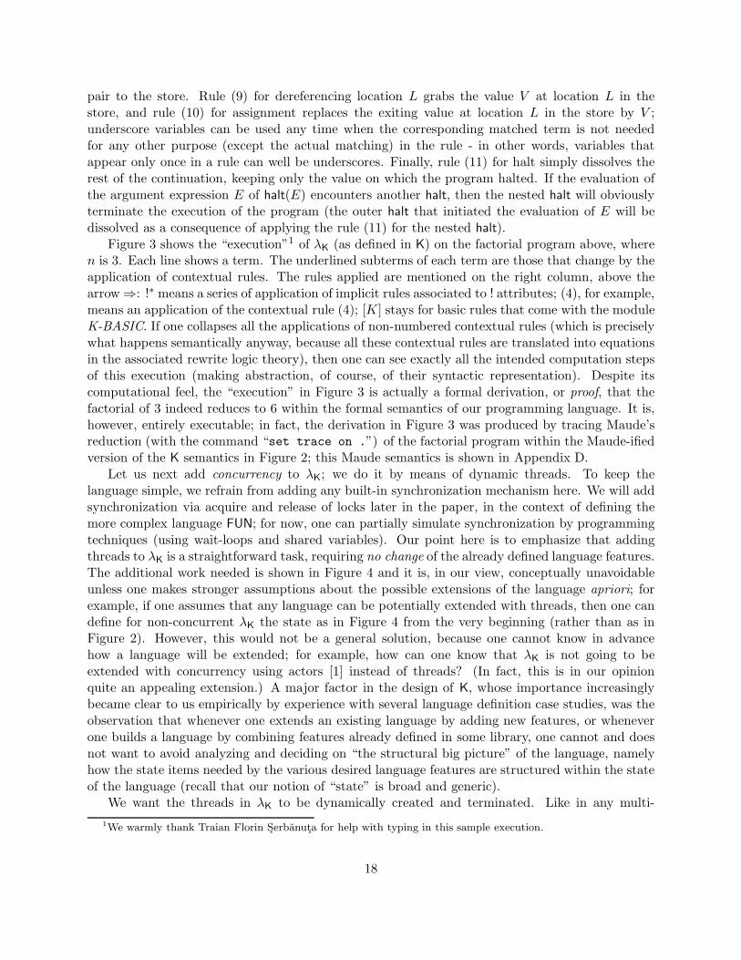
pair to the store. Rule (9) for dereferencing location L grabs the value V at location L in thestore, and rule (10) for assignment replaces the exiting value at location L in the store by V ;underscore variables can be used any time when the corresponding matched term is not neededfor any other purpose (except the actual matching) in the rule - in other words, variables thatappear only once in a rule can well be underscores. Finally, rule (11) for halt simply dissolves therest of the continuation, keeping only the value on which the program halted. If the evaluation ofthe argument expression E of halt(E) encounters another halt, then the nested halt will obviouslyterminate the execution of the program (the outer halt that initiated the evaluation of E will bedissolved as a consequence of applying the rule (11) for the nested halt).

Figure 3 shows the “execution”1 of λK (as defined in K) on the factorial program above, wheren is 3. Each line shows a term. The underlined subterms of each term are those that change by theapplication of contextual rules. The rules applied are mentioned on the right column, above thearrow⇒: !∗ means a series of application of implicit rules associated to ! attributes; (4), for example,means an application of the contextual rule (4); [K] stays for basic rules that come with the moduleK-BASIC. If one collapses all the applications of non-numbered contextual rules (which is preciselywhat happens semantically anyway, because all these contextual rules are translated into equationsin the associated rewrite logic theory), then one can see exactly all the intended computation stepsof this execution (making abstraction, of course, of their syntactic representation). Despite itscomputational feel, the “execution” in Figure 3 is actually a formal derivation, or proof, that thefactorial of 3 indeed reduces to 6 within the formal semantics of our programming language. It is,however, entirely executable; in fact, the derivation in Figure 3 was produced by tracing Maude’sreduction (with the command “set trace on .”) of the factorial program within the Maude-ifiedversion of the K semantics in Figure 2; this Maude semantics is shown in Appendix D.

Let us next add concurrency to λK; we do it by means of dynamic threads. To keep thelanguage simple, we refrain from adding any built-in synchronization mechanism here. We will addsynchronization via acquire and release of locks later in the paper, in the context of defining themore complex language FUN; for now, one can partially simulate synchronization by programmingtechniques (using wait-loops and shared variables). Our point here is to emphasize that addingthreads to λK is a straightforward task, requiring no change of the already defined language features.The additional work needed is shown in Figure 4 and it is, in our view, conceptually unavoidableunless one makes stronger assumptions about the possible extensions of the language apriori; forexample, if one assumes that any language can be potentially extended with threads, then one candefine for non-concurrent λK the state as in Figure 4 from the very beginning (rather than as inFigure 2). However, this would not be a general solution, because one cannot know in advancehow a language will be extended; for example, how can one know that λK is not going to beextended with concurrency using actors [1] instead of threads? (In fact, this is in our opinionquite an appealing extension.) A major factor in the design of K, whose importance increasinglybecame clear to us empirically by experience with several language definition case studies, was theobservation that whenever one extends an existing language by adding new features, or wheneverone builds a language by combining features already defined in some library, one cannot and doesnot want to avoid analyzing and deciding on “the structural big picture” of the language, namelyhow the state items needed by the various desired language features are structured within the stateof the language (recall that our notion of “state” is broad and generic).

We want the threads in λK to be dynamically created and terminated. Like in any multi-1We warmly thank Traian Florin Serbanuta for help with typing in this sample execution.

18

eval((λr . (λg . g(3− 1, g))(λm, h . if m > 1 then (λd.h(m− 1, h) (r := (∗r) ∗m)) else halt (∗r))) (ref 3))!∗⇒

eval(((λr . ((λg . (g, (3, 1) �−, g) � app), λm, h .%G) � app), 3 � ref) � app)(1)⇒

result(k(((λr . ((λg . (g, (3, 1) �−, g) � app), λm, h . %G) � app), 3 � ref) � app) store(.) nextLoc(0) env(.))[K]⇒

result(k((λr . ((λg . (g, (3, 1) �−, g) � app), λm, h . %G) � app) � (3 � ref, ·) � app) store(.) nextLoc(0) env(.))(4)⇒

result(k(closure(r, ((λg . (g, (3, 1) �−, g) � app), λm, h . %G) � app, ·) � (3 � ref, ·) � app) store(.) nextLoc(0) env(.))[K]⇒

result(k(3 � ref � (·, closure(r, ((λg . (g, (3, 1) �−, g) � app), λm, h . %G) � app, ·)) � app) store(.) nextLoc(0) env(.))(8),[K]⇒

result(k(loc(0) � (·, closure(r, ((λg.(g, (3, 1)�−, g)�app), λm, h.%G)�app, ·))�app) store((0, 3)) nextLoc(1) env(.))[K]⇒

result(k((closure(r, ((λg.(g, (3, 1)�−, g)�app), λm, h.%G)�app, ·), loc(0))�app) store((0, 3) ·) nextLoc(1) env(.))(5),[K]⇒

result(k((λg.(g, ((3, 1) �−), g) � app) � (λm, h.%G, .) � app � (.)) store((0, 3)(1, loc(0))) nextLoc(2) env((r, 1)))(4),[K]⇒

result(k((closure(g, (g, ((3, 1) �−), g) � app, (r, 1)), %C1) � app � (.)) store((0, 3)(1, loc(0)) ·) nextLoc(2) env((r, 1)))(5),[K]⇒

result(k(g � (((3, 1) �−), g, .) � app � ((r, 1)) � (.)) store((0, 3)(1, loc(0))(2, %C1)) nextLoc(3) env((g, 2)(r, 1)))(3),[K]⇒

result(k((%C1, 2, %C1) � app � ((r, 1)) � (.)) store((0, 3)(1, loc(0))(2, %C1) ·) nextLoc(3) env((g, 2)(r, 1)))(5),[K]⇒

result(k(m � (1, .) �> � %IF � ((g, 2)(r, 1)) � ((r, 1)) � (.)) %S1)(3),[K]⇒

result(k(bool(true) � %IF � %e1) %S1)(6),[K]⇒

result(k((λd.(h, ((m, 1) �−), h) � app) � ((r, ((r � ∗), m) � ∗) �:=, .) � app � %e1) %S1)(4,3),[K]⇒

result(k(loc(0) � ∗� (m, .) � ∗� (., loc(0)) �:=� (., %C2) � app � %e1) %S1)(9),[K]⇒

result(k(m � (., 3) � ∗� (., loc(0)) �:=� (., %C2) � app � %e1) %S1)(3),[K]⇒

result(k((loc(0), 6) �:=� (., %C2) � app � %e1) store((0, 3) %s1 ) nextLoc(5) env((h, 4)(m, 3)(r, 1)))(10),[K]⇒

result(k((%C2, 6) � app � %e1) store((0, 6) %s1 ·) nextLoc(5) env((h, 4)(m, 3)(r, 1)))(5),[K]⇒

result(k(h � (((m, 1) �−), h, .) � app � %e2) store((0, 6) %s1 (5, 6)) nextLoc(6) env((d, 5)(h, 4)(m, 3)(r, 1)))(3),[K]⇒

result(k((%C1, 1, %C1) � app � %e2) store((0, 6) %s1 (5, 6) ·) nextLoc(6) env((d, 5)(h, 4)(m, 3)(r, 1)))(5),[K]⇒

result(k(m � (1, .) �> � %IF � %e3) %S2)(3),[K]⇒

result(k(bool(false) � %IF � %e3) %S2)(7)⇒

result(k(r � ∗� halt � %e3) %S2)(3)⇒

result(k(loc(0) � ∗� halt � %e3) %S2)(9)⇒

result(k(6 � halt � %e3) %S2)(11)⇒

result(k(6) %S2)(2)⇒

6

%IF stands for if((λd.(r, (r � ∗, m) � ∗) � :=)((h, (m, 1) �−, h) � app), r � ∗� halt)%G stands for (m, 1) � > � %IF%C1 stands for closure(m, h, %G, (r, 1))%S1 stands for store((0, 3) %s1 ) nextLoc(5) env((h, 4)(m, 3)(r, 1)))%e1 stands for ((g, 2)(r, 1)) � ((r, 1)) � (.)%C2 stands for closure(d, (h, ((m, 1) �−), h) � app, (h, 4)(m, 3)(r, 1))%s1 stands for (1, loc(0))(2, %C1)(3, 2)(4, %C1)%e2 stands for ((h, 4)(m, 3)(r, 1)) � %e1%e3 stands for ((d, 5)(h, 4)(m, 3)(r, 1)) � %e2%S2 stands for store((0, 6) %s1 (5, 6)(6, 1)(7, %C1)) nextLoc(8) env((h, 7)(m, 6)(r, 1))

Figure 3: Sample run of the factorial program in the executable semantics of λK in K.

19

The definition of λK in Figure 2needs to be changed as follows:1) replace structural operators with

the ones in the picture to the right2) replace definition of eval as below3) add two more rules, as below:

a) one for creation of threads; andb) one for termination of threads

No other changes needed.

Structural operations

Continuation

k

Env

ThreadState Nat

env

LocValSet

State

storenextLocthread *

eval(E)result(thread(k(E) env(·)) store(·) nextLoc(0))

( 1)

spawn :Exp→ Expdie : · → ContinuationItem

}⎧⎪⎪⎪⎪⎨⎪⎪⎪⎪⎩

thread(k(spawn E

0〉 env(Env)) ·

thread(k(E � die) env(Env))(12)

thread〈k(V : Val � die)〉·

(13)

Figure 4: Adding threads to λK

threaded language, threads in λK may share memory locations. More precisely, a newly createdthread shares the same environment as its parent thread. Therefore, accesses (reads or writes)to variables shared by different threads may lead to non-deterministic behaviors of programs (inparticular to data-races). All these suggest to the language designer the state structure depictedin Figure 4 for multi-threaded λK. Its state therefore contains, besides a store and a next availablelocation like in the non-concurrent version, an arbitrary number of threads. The star (�) on thearrow labeled thread in the graph in Figure 4 means that corresponding subterms wrapped by thestate constructor operator thread can appear multiple times in the state — in this case, reflectingthe fact that the number of threads created during the execution of a program varies. The starannotation happens to be irrelevant in the definition of multi-threaded λK, but in other languagedefinitions it may play a critical role in the disambiguation of the context transformation processdiscussed next. Each subterm in the state soup wrapped by a thread construct (i.e., each thread)contains a continuation k(...) and an environment env(...).

The next step is to create the initial state of a program. Unlike in non-concurrent λK wherethe initial state contained the continuation and the environment at the same top level as the storeand the next available location, in multi-threaded λK the initial state should contain one thread atthe same top level as the store and the next available location, but the continuation associated tothe program to evaluate as well as its corresponding (empty) environment should be contained aspart of that thread, rather than at the top level (so we have a “nested soup”). This way, severalthreads with their corresponding continuations and environments can be unambiguously created,

20

terminated and accessed dynamically. The semantics of the operation eval needs to be changednow to appropriately initiate the evaluation of its argument expression taking into considerationthe new initial state.

An intriguing observation at this stage is that many of the contextual rules in Figure 2 do notparse anymore because of the new state structure, and so does the sample execution in Figure 3.Therefore, it looks as if the addition of threads to λK broke the modularity of the other languagefeature definitions. That would be, indeed, the case in the context of most language definitionalframeworks, including SOS as well as plain rewrite logic definitions of languages. However, in Kwe need to change no existing definitions of other language features, even though they were definedbefore the state structure of multithreaded λK was known. That is thanks to one of the mostimportant features of K, called context transformer and explained next.

In K, the structural operators play a crucial role in the definition of a language. Many ofthe contextual rules in a K definition of a language are incomplete unless full knowledge of thestate structure is available. That incompleteness allows language designers to only mention therelevant part of the state when defining the semantics of each feature. An advantage of rewritelogic definitions compared to SOS definitions is that in a rewrite rule one needs only mentionthe local structure of a subterm on which a transformation is applied, while in traditional SOSdefinitions one needs to mention the entire state, or configuration, even though one wants to changeonly a very small portion of it. Thanks also to matching modulo associativity, commutativity andidentity which bring additional modularity to language definitions, rewriting logic allows for elegantand compact definitions even of complex features of languages [19, 18]. However, rewriting logicimposes well-formedness of its rewrite rules w.r.t. signatures, so definitions of features cannot beeasily transported from one language to another when the structure of the state changes. K’scontext transformers address precisely this limitation of rewriting logic. At this moment we solveall the context transformers statically because we assume that the structure of the state does notchange. However, one could also imagine, at least in principle, more complex situations in whichthe structure of the state would change dynamically; in such a case one could informally think ofcontext transformers as of matching modulo structure.

Context transformers will be explained in detail later in the paper; we here only discuss theirapplication on multi-threaded λK. Intuitively, once all the structural operators are known, suchas in the pictures in Figures 2 and 4, the contextual rules need not mention the complete “path”to each operation that appears in a rule, because that path can be inferred automatically andunambiguously from the declared structure of the state. For example, consider rule (2) in Figure 2defined for non-concurrent λK, but when the structure of the language changes as in Figure 4. Thisrule obviously does not parse anymore, because result expects an argument of sort State which,because of the structural operators in Figure 4, can only be constructed with state constructorsthread(...), store(...), and nextLoc(...); therefore, there is no k(...) construct at the top level ofthe state anymore, so result〈k(V )〉 naturally does not parse. However, the crucial observationis that there is a unique way to have k(V ) make sense in a term below the operation result :when k(V ) is part of a thread state, wrapped by the operator thread. Therefore, by taking thestructural operators into account, one can automatically and unambiguously transform result〈k(V )〉into result〈thread〈k(V )〉〉, the latter making now full sense in the new language definition. Similarly,with the new state structure in Figure 4, one can automatically transform rule (3) in Figure 2 into

21

thread〈k(XV

〉 env〈(X,L)〉〉 store〈(L, V )〉.

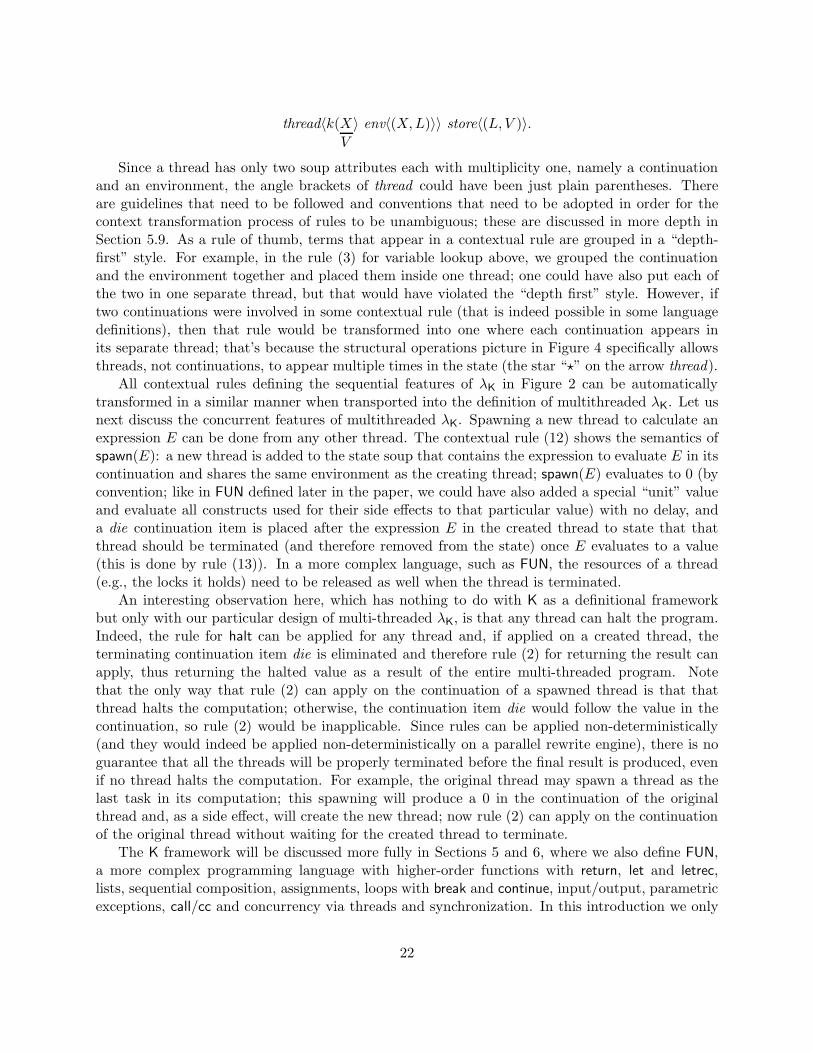
Since a thread has only two soup attributes each with multiplicity one, namely a continuationand an environment, the angle brackets of thread could have been just plain parentheses. Thereare guidelines that need to be followed and conventions that need to be adopted in order for thecontext transformation process of rules to be unambiguous; these are discussed in more depth inSection 5.9. As a rule of thumb, terms that appear in a contextual rule are grouped in a “depth-first” style. For example, in the rule (3) for variable lookup above, we grouped the continuationand the environment together and placed them inside one thread; one could have also put each ofthe two in one separate thread, but that would have violated the “depth first” style. However, iftwo continuations were involved in some contextual rule (that is indeed possible in some languagedefinitions), then that rule would be transformed into one where each continuation appears inits separate thread; that’s because the structural operations picture in Figure 4 specifically allowsthreads, not continuations, to appear multiple times in the state (the star “�” on the arrow thread).

All contextual rules defining the sequential features of λK in Figure 2 can be automaticallytransformed in a similar manner when transported into the definition of multithreaded λK. Let usnext discuss the concurrent features of multithreaded λK. Spawning a new thread to calculate anexpression E can be done from any other thread. The contextual rule (12) shows the semantics ofspawn(E): a new thread is added to the state soup that contains the expression to evaluate E in itscontinuation and shares the same environment as the creating thread; spawn(E) evaluates to 0 (byconvention; like in FUN defined later in the paper, we could have also added a special “unit” valueand evaluate all constructs used for their side effects to that particular value) with no delay, anda die continuation item is placed after the expression E in the created thread to state that thatthread should be terminated (and therefore removed from the state) once E evaluates to a value(this is done by rule (13)). In a more complex language, such as FUN, the resources of a thread(e.g., the locks it holds) need to be released as well when the thread is terminated.

An interesting observation here, which has nothing to do with K as a definitional frameworkbut only with our particular design of multi-threaded λK, is that any thread can halt the program.Indeed, the rule for halt can be applied for any thread and, if applied on a created thread, theterminating continuation item die is eliminated and therefore rule (2) for returning the result canapply, thus returning the halted value as a result of the entire multi-threaded program. Notethat the only way that rule (2) can apply on the continuation of a spawned thread is that thatthread halts the computation; otherwise, the continuation item die would follow the value in thecontinuation, so rule (2) would be inapplicable. Since rules can be applied non-deterministically(and they would indeed be applied non-deterministically on a parallel rewrite engine), there is noguarantee that all the threads will be properly terminated before the final result is produced, evenif no thread halts the computation. For example, the original thread may spawn a thread as thelast task in its computation; this spawning will produce a 0 in the continuation of the originalthread and, as a side effect, will create the new thread; now rule (2) can apply on the continuationof the original thread without waiting for the created thread to terminate.

The K framework will be discussed more fully in Sections 5 and 6, where we also define FUN,a more complex programming language with higher-order functions with return, let and letrec,lists, sequential composition, assignments, loops with break and continue, input/output, parametricexceptions, call/cc and concurrency via threads and synchronization. In this introduction we only

22

wanted to emphasize that once learned, K is simple, natural, and leads to compact and easy tounderstand and read language definitions. An interesting feature of K that we have not discussedso far but which is also worthwhile mentioning, is the distinction that it makes among contextualrules. These can be:

• Structural, or non-computational. These are rules whose only role is to allow modifications ofthe structure of the state, so that other contextual rules that have computational meaning canapply. For example, the rules generated automatically by K for the strictness attributes (“!”)as well as rule (1) are all structural, their role being to prepare the expression for evaluationby prioritizing the subexpressions that need to be evaluated first. Also, all the set and listimplicit associativity and commutativity equations are structural, having no computationalmeaning.

• Computational. These are rules that each captures precisely one intended execution step ofthe program. All numbered rules in the definition of λK except (1) are computational.

• Non-deterministic. These are rules that can potentially change the deterministic behavior ofa program. If a language is sequential and deterministic, then there is no need to declare anycontextual rule to be non-deterministic, because the rules are expected to be Church-Rosseron the terms of interest (well-formed programs). However, if a language admits concurrency,then some rules may lead to non-deterministic executions; for example, reads and writes ofmemory locations, or acquires of locks.

Non-deterministic rules are always a (typically quite small) subset of the computational rules.The structural and computational declarations of contextual rules are modular, in the sense thatone does not need knowledge about the entire language in order to declare a rule structural orcomputational. However, the non-deterministic declaration of rules is trickier and needs globalinformation about the program. For example, one cannot know when one defines a variable lookuprule (3) whether the defined language is concurrent or not; if it is, then that rule needs to be declarednon-deterministic. Also, it is impossible to identify the non-deterministic rules automatically ingeneral (this problem is harder than testing confluence).

K can be all resolved statically, so a definition of a language in K is a rewrite logic specification.One subtle aspect of the translation of K into rewriting logic is to decide which contextual rulestranslate into equations and which into rewrite rules (see Section 3 for the semantic distinctionbetween the two). In general, if one is interested in obtaining just one interpreter or a dynamic se-mantics for the language, then one can translate all the computational contextual rules into rewriterules and the non-computational ones into equations. If formal analysis of programs is of interest,then one may want to reduce the number of rewrite rules to a minimum; this can be done bytransforming only the non-deterministic contextual rules into rewrite rules. Since rewriting logicis efficiently executable (rewrite engines such as ASF+SDF and Maude are quite fast), relativelyefficient interpreters are obtained for free from such formal language definitions. However, K speci-fications follow a certain definitional methodology which identifies them as particular rewrite logicspecifications. Therefore, one should be able to execute these K definitions more efficiently usingsome specialized rewrite engines or compilers than using general purpose rewrite engines such asASF+SDF or Maude. Some preliminary experiments have been made showing that that is indeedthe case; Section 11 gives more details.

Also, formal analysis tools for rewrite logic specifications, such as those of Maude [5] (e.g., modelcheckers), translate into corresponding tools for languages defined using the presented technique.

23

Also, since rewriting logic is a computational logical framework with both initial model semanticsand formal analysis techniques for initial models, the presented framework can also serve as afoundation for program verification. The technique presented here, or previous versions of it, hasbeen used to define language features including type inference, object-orientation and subtyping,concurrency, etc., as well as large fragments of real programming languages, such as the λ-calculus,System F, Beta, Haskell, Java, LLVM, LISP, Python, Pict, Ruby, and Smalltalk [24].As discussed in [7] and Section 10, the model checker obtained for free from the formal definitionof Java compares favorably with two state of the art Java model checkers.

24

3 Rewriting Logic

The language definitional framework proposed in this paper can be presented and understoodin isolation, like SOS or reduction semantics, and implemented following different programmingparadigms. However, as mentioned previously, we prefer to present it via an automatic translationto term rewriting modulo equations or to rewriting logic, for two reasons:

1. to make it clear upfront that we inherit all the good properties of these well understood andgeneric computational frameworks, and

2. to use at no additional effort the remarkable rewrite-based tool support developed over thelast few decades.

We here informally recall some basic notions of rewriting logic and of its important sublogic calledequational logic, together with operational intuitions of term rewriting modulo equations.

3.1 Equational Logics

Equational logic is perhaps the simplest logic having the full expressivity of computability [2].One can think of it as a logic of “term replacement”: terms can be replaced by equal terms inany context. An equational specification is a pair (Σ, E), where Σ is a set of “uninterpreted”operations, also called its “syntax”, and E is a set of equations of the form (∀X) t = t′ constrainingthe syntax, where X is some set of variables and t, t′ are well-formed terms over variables in Xand operations in Σ. Equational logics can be many-sorted [10] (operations in Σ have argumentsof specific sorts), or even order-sorted [11], i.e., sorts come with a partial order on them; we useorder-sorted specifications in this paper. Also, equations can be conditional, where the conditionis a (typically finite) set of pairs u = u′ over the same variables X. We write conditional equations(of finite condition) using the notation (∀X) t = t′ ⇐ u1 = u′1 ∧ · · · ∧ un = u′n.

Models of an equational specification (Σ, E) interpret sorts into sets of values and operations inΣ into corresponding functions satisfying all the equations in E, where a model satisfies an equationif and only if the two terms evaluate to the same value for any assignment of their variables tovalues in the model. Models are also called Σ-algebras and it is customary to regard them as“realizations”, or even “implementations”, of the equational specifications they satisfy. Equationaldeduction is complete and consists of five natural deduction rules, namely reflexivity, symmetry,transitivity, congruence and substitution. We write E Σ e if the equation e can be derived withthese rules from (Σ, E). Among the variety of models of an equational specification, there is onewhich, up-to-an-isomorphism, captures precisely the intended meaning of the specification: itsinitial model. Because of the “all-in-one and one-in-all” flavor and properties of initial algebras,as well as because any computable domain can be shown isomorphic to a (restricted) initial modelover a finite equational specification [2], initial algebra semantics [12] was introduced in 1977 as atheoretically self-contained approach to (non-concurrent) programming language semantics.

3.2 Term Rewriting

Term rewriting is a related approach in which equations are oriented left-to-right, written (∀X) l→r and called rewrite rules, and can be applied to a term t at any position where l matches as follows:find some subterm t′ of t, that is, t = c[t′] for some context c, which is an instance of the left-hand-side term (lhs) of some rewrite rule (∀X) l → r, that is, t′ = θ(l) for some variable assignment θ,

25

and replace t′ by θ(r) in t. This way, the term t can be continuously transformed, or rewritten.A pair (Σ, R), where R is a set of such oriented rewrite rules, is called a rewrite system. Thecorresponding term rewriting relation is written →R and its inverse is written ←R. If no rule in Rcan rewrite a Σ-term, than that term is said to be in normal form w.r.t. R.

Term rewriting can be used as an operational mechanism to perform equational deduction.Specifically, E Σ (∀X) t = t′ if and only if t (→RE

∪ ←RE)∗ t′, where RE is the set of rewrite

rules obtained by orienting all the equations in E from left to right. Therefore, term rewriting isas powerful as equational deduction if used in both directions. However, in practice term rewritingis used as a heuristic for equational deduction. A very common case is to attempt the task E Σ

(∀X) t = t′ by showing t →∗RE· ←∗RE

t′, i.e., by reducing both t and t′ to some common termusing (Σ, RE). In some cases, for example when (Σ, RE) is confluent and terminates, this becomesa semi-decision procedure for equational deduction.

There are many software systems that either specifically implement term rewriting efficiently,known also as rewrite engines, or that support term rewriting as part of a more complex func-tionality. Any of these systems can be used as an underlying platform for execution and analysisof programming languages defined using the technique and the formalism proposed in this paper.Without attempting to be exhaustive, we here only mention (alphabetically) some engines thatwe are more familiar with, noting that many functional languages and theorem provers providesupport for term rewriting as well: ASF/SDF [27], CafeOBJ [6], Elan [3], Maude [5], OBJ [13],Stratego [28]. Some of these can achieve remarkable speeds on today’s machines, in the order ofmillions or tens of millions of rewrite steps per second. Many engines store terms as directed acyclicgraphs (DAGs), so applications of rewrite rules consist in many cases of just permuting pointers,which can indeed be implemented quite efficiently. In our language definitions, we often place orremove environments or continuations onto other structures; even though these may look like heavyoperations, in fact these do nothing but save or remove pointers to subterms when these definitionsare executed.

Because of the forward chaining executability of term rewriting and also because of these efficientrewrite engines, equational specifications are often called executable. As programming languagestend to be increasingly more abstract due to the higher speeds of processors, and as specificationlanguages tend to be provided with faster execution engines, the gap between executable specifi-cations and implementations, in case there has ever been any, is becoming visibly narrower. Forexample, we encourage the curious reader to specify the factorial operation equationally as follows(s is the Peano “successor”)

0! = 1s(N)! = s(N) ∗N !

in a fast rewrite engine like Maude, versus implementing it in programming languages like ML orScheme. In our experiments, the factorial of 50,000, a number of 213,237 digits, was calculated in18.620 seconds by the executable equational engine Maude and in 19.280 and 16.770 seconds bythe programming languages ML and Scheme, respectively. In case one thinks that the efficiencyof builtin libraries should not be a factor in measuring the efficiency of a system, one can definepermutations equationally instead, for example as follows

Sorts and SubsortsNat < Permutation < Permutations

Operations, : Permutation Permutation → Permutation [assoc]

26

; : Permutations Permutations → Permutations [assoc]perm : Nat → Permutationsinsert : Nat Permutations → Permutationsmap-cons : Nat Permutations → Permutations

Equationsperm(1) = 1perm(s(N)) = insert(s(N), perm(N))insert(N , (P :Permutation ; Ps:Permutations)) = insert(N ,P ) ; insert(N ,Ps)insert(N, (M,P’)) = (N,M,P’) ; map-cons(M, insert(N,P’))insert(N, M) = (N,M) ; (M,N)map-cons(M, (P ; Ps)) = map-cons(M, P) ; map-cons(M, Ps)map-cons(M, P) = (M,P)

The above is an order-sorted equational specification; for readability, we used the mixfix notation foroperation declarations (underscores are argument placeholders) which is supported by many rewriteengines. Also, we declared the list constructor operations with the attribute [assoc]. Semanticallythis is equivalent to giving the equation of associativity, but rewrite engines typically use thisinformation to enable specialized algorithms for rewriting and matching modulo associativity; wewill discuss matching modulo attributes like associativity, commutativity and identity in moredepth shortly. Like in the previous example, we assumed some builtin natural numbers comingwith a successor operation.

In our experiments with permutations, the executable equational specifications outperformedthe implementations. Maude took 61 seconds to “calculate” permutations of 10, while ML andScheme took 83 and 92 seconds, respectively. None of these systems were able to calculate per-mutations of 11. These experiments have been performed on a 2.5GHz Linux machine with 3.5GBof memory, and we2 used Maude 2.0, PolyML and PLT Scheme (specifically mzscheme), all pro-viding libraries for large numbers. These simplistic experiments should by no means be consideredconclusive; our measurements favoring executable specifications may be due to fortunate uses ofdata-structures in the Maude implementation, or even to our lack of usage of Scheme and ML attheir maximum efficiency. While more extensive comparisons and analyses would be interestingand instructive, this is not our goal here; nor to unreasonably claim that executable specificationswill ever outperform implementations. All we are trying to say is that the pragmatic, semantics-reluctant language designer, can safely regard the subsequent semantic definitions of languagefeatures as implementations, in spite of their conciseness and mathematical flavor.

NEXT-VERSION: discuss the examples with white/black balls and with bubble sorting

3.3 Rewriting Logic

While equational logic and its execution via term rewriting provide as powerful computationalproperties as one can get in a sequential setting, these were not designed to specify or reasonabout concurrent systems. The initial algebra model of an equational specification collapses allthe computationally equivalent terms, but it does not say anything about evolution of terms underconcurrent transitions. There are at least two broad directions of research on the subject of speci-fying non-deterministic and/or concurrent systems [30]. One builds upon the Platonist belief that

2Warmest thanks to Mark Hills who helped with these experiments.

27

models are deterministic, but, by making use of underspecification, one never knows precisely inwhich model one is3. While underspecification is a very powerful approach in semantics, in our pro-gramming language definitional framework it suffers from a crucial impediment: it is not executableenough to allow one to execute actual concurrent programs. Nevertheless, we will make intensiveuse of underspecification by not specifying implementation details of programming languages (suchas how environments, stores, lists or stacks are implemented). Another direction of thought inconcurrency is to allow non-determinism in models, typically by means of non-deterministic tran-sitions. Specifications become executable now, because all what one needs to do is to randomlypick some transition when more are possible. This is similar to what thread/process schedulers doin concurrent computer systems.

To properly define and analyze (concurrent) programming languages formally, we need a frame-work which provides natural support for concurrency. In other words, we would like a frameworkin which we can state what programming language features are meant to do without artificial en-codings of these due to artifacts of the underlying definitional framework. For example, we wouldconsider it “unnatural” to define, or simulate, a particular “thread or process scheduler” in orderto define a concurrent language, just because the underlying definitional framework is inherentlysequential. Since both underspecification and non-deterministic transitions seem important forcapturing the meaning of programming language features, we would like an underlying frameworkthat supports both.

Rewriting logic [17] is a logic for concurrency, which should not be confused with term rewriting.A rewrite specification, or theory, is a triple (Σ, E,R), where (Σ, E) is an equational specificationand R is a set of rewrite rules. Rewriting logic therefore extends equational logic with rewrite rules,allowing one to derive both equations and rewrites (or transitions). Deduction remains the samefor equations, but the symmetry rule is dropped for rewrite rules. Models of rewrite theories are(Σ, E)-algebras enriched with transitions satisfying all the rewrite rules in R. In our context, theequational part of a rewrite theory is allowed to “underspecify” features as far as the specificationremains executable. Interestingly, rewrite theories also have initial models, consisting of termmodels factored by the equational derivability relation and enriched with appropriate transitionsbetween the equational equivalence classes. They also follow the slogan “no junk, no confusion”,but extend it also w.r.t. reachability of terms via transitions.

Rewriting logic is a framework for true concurrency. The reader interested in details is referredto [17]. We here only discuss this by means of examples. Suppose that (Σ, E,R) is the followingrewrite theory:

Σ:sort Stateoperation ∅ : → Stateoperation : State × State→ Stateoperation 0 : → Stateoperation 1 : → State

E:equation (∀S : State) ∅ S = S

3There is some resemblance here to the idea of parallel worlds promoted by Giordano Bruno 400+ years ago inhis book “The Infinity, the Universe and Its Worlds”. He was sentenced to death by fire by the Inquisition for his“heretic” thinking.

28

equation (∀S1, S2 : State) S1 S2 = S2 S1

equation (∀S1, S2, S3 : State) (S1 S2) S3 = S1 (S2 S3)

R:rule r1 : 0⇒ 1rule r2 : 1⇒ 0

The two equations state the associativity and commutativity of the binary “ ” operator, thusmaking it a multi-set operator, and the two rules flip the two constants 0 and 1. If one starts withan initial term as a multi-set containing 0 and 1 constants, then the rules r1 and r2 can applyconcurrently. For example, if the initial term is the multi-set 0 1 0 1 0 then three instances of r1

and two of r2 can apply in parallel and transform the multi-set into 1 0 1 0 1. Note, however,that there is no requirement on the number of rewrites applied concurrently; for example, one canapply only the instances of r1, or only one instance of r1 and one of r2, etc. Consequently, on amulti-set of 0 and 1 constants, the rewrite theory above manifests all possible concurrent behaviors,not only those following an interleaving semantics. And indeed, if one “executes” this specificationon a machine with an arbitrarily large number of processors, then one can observe any of theseconcurrent behaviors. Parallel execution of rewrite logic specifications is an important aspect ofour language definitions; we will rediscuss it.

One can regard a rewrite logic specification as a compact means to encode transition systems,namely one that has the capability to generate for any given term a transition system manifestingall its “concurrent” behaviors. The states of that transition system are the terms to which theoriginal term can evolve by iterative applications of rewrite rules; the equations are used to keepthe states in canonical forms (in this case as AC multi-sets, but in general as any terms which arenot reducible by applying equations from left to right – modulo particular axioms, such as ACI)and the rules are used to generate transitions (in this case the rules are not parametric, but ingeneral they can have variables, each rule corresponding to a recursively enumerable set of groundtransitions).

Given a rewrite logic specification and an initial term, the corresponding transition system mayor may not need to be generated explicitly. For example, if one is interested in one execution of thespecification on that term, then one only needs to generate one path in the transition system. Ifone is interested in testing whether a particular term can be reached (reachability analysis), thenone can only generate the transition system by need, for example following a breadth-first strategy.However, if one is interested in checking some complex property against all possible executions(model-checking) then one may need to generate the entire transition system. Interestingly, one canregard a concurrent programming language also as a means to encode transition systems, namelyone taking a program and, depending upon the intended purpose, generate one path, part of, orthe entire transition system comprising all behaviors of that program. Thus, that programminglanguages can be given a rewriting logic semantics should come as no surprise. What may seemsurprising in the sequel is the simplicity of such language definitions when one uses the K framework.

All rewrite engines, by their nature, generate one (finite or infinite) path in the transition systemof a term when requested to reduce that term. Therefore, we can use any of these rewrite engines toexecute our K specifications, thus converting them into interpreters for the programming languagesdefined in K. The Maude system also supports breadth-first exploration of the state space of thetransition system of a term, as well as linear temporal logic (LTL) model checking. Using thesefeatures one can, for example, show that in the example above it is possible to start with the stateof zeros 0 0 0 0 0 and reach a state of just ones; also, using the model checker one can show that it

29

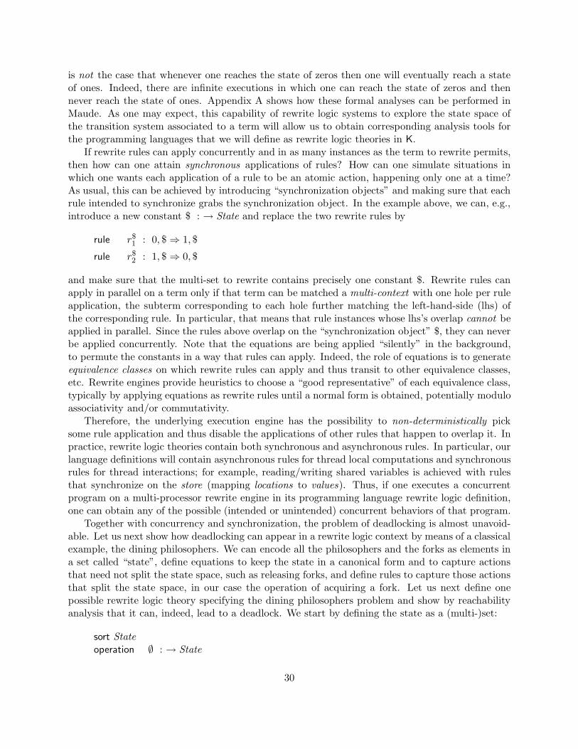
is not the case that whenever one reaches the state of zeros then one will eventually reach a stateof ones. Indeed, there are infinite executions in which one can reach the state of zeros and thennever reach the state of ones. Appendix A shows how these formal analyses can be performed inMaude. As one may expect, this capability of rewrite logic systems to explore the state space ofthe transition system associated to a term will allow us to obtain corresponding analysis tools forthe programming languages that we will define as rewrite logic theories in K.

If rewrite rules can apply concurrently and in as many instances as the term to rewrite permits,then how can one attain synchronous applications of rules? How can one simulate situations inwhich one wants each application of a rule to be an atomic action, happening only one at a time?As usual, this can be achieved by introducing “synchronization objects” and making sure that eachrule intended to synchronize grabs the synchronization object. In the example above, we can, e.g.,introduce a new constant $ : → State and replace the two rewrite rules by

rule r$1 : 0, $⇒ 1, $

rule r$2 : 1, $⇒ 0, $

and make sure that the multi-set to rewrite contains precisely one constant $. Rewrite rules canapply in parallel on a term only if that term can be matched a multi-context with one hole per ruleapplication, the subterm corresponding to each hole further matching the left-hand-side (lhs) ofthe corresponding rule. In particular, that means that rule instances whose lhs’s overlap cannot beapplied in parallel. Since the rules above overlap on the “synchronization object” $, they can neverbe applied concurrently. Note that the equations are being applied “silently” in the background,to permute the constants in a way that rules can apply. Indeed, the role of equations is to generateequivalence classes on which rewrite rules can apply and thus transit to other equivalence classes,etc. Rewrite engines provide heuristics to choose a “good representative” of each equivalence class,typically by applying equations as rewrite rules until a normal form is obtained, potentially moduloassociativity and/or commutativity.

Therefore, the underlying execution engine has the possibility to non-deterministically picksome rule application and thus disable the applications of other rules that happen to overlap it. Inpractice, rewrite logic theories contain both synchronous and asynchronous rules. In particular, ourlanguage definitions will contain asynchronous rules for thread local computations and synchronousrules for thread interactions; for example, reading/writing shared variables is achieved with rulesthat synchronize on the store (mapping locations to values). Thus, if one executes a concurrentprogram on a multi-processor rewrite engine in its programming language rewrite logic definition,one can obtain any of the possible (intended or unintended) concurrent behaviors of that program.

Together with concurrency and synchronization, the problem of deadlocking is almost unavoid-able. Let us next show how deadlocking can appear in a rewrite logic context by means of a classicalexample, the dining philosophers. We can encode all the philosophers and the forks as elements ina set called “state”, define equations to keep the state in a canonical form and to capture actionsthat need not split the state space, such as releasing forks, and define rules to capture those actionsthat split the state space, in our case the operation of acquiring a fork. Let us next define onepossible rewrite logic theory specifying the dining philosophers problem and show by reachabilityanalysis that it can, indeed, lead to a deadlock. We start by defining the state as a (multi-)set:

sort Stateoperation ∅ : → State

30

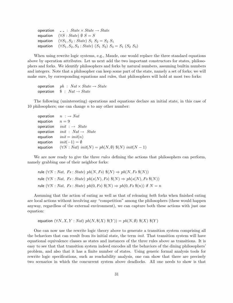
operation : State × State→ Stateequation (∀S : State) ∅ S = Sequation (∀S1, S2 : State) S1 S2 = S2 S1

equation (∀S1, S2, S3 : State) (S1 S2) S3 = S1 (S2 S3)

When using rewrite logic systems, e.g., Maude, one would replace the three standard equationsabove by operation attributes. Let us next add the two important constructors for states, philoso-phers and forks. We identify philosophers and forks by natural numbers, assuming builtin numbersand integers. Note that a philosopher can keep some part of the state, namely a set of forks; we willmake sure, by corresponding equations and rules, that philosophers will hold at most two forks:

operation ph : Nat× State→ Stateoperation $ : Nat→ State

The following (uninteresting) operations and equations declare an initial state, in this case of10 philosophers; one can change n to any other number:

operation n : → Natequation n = 9operation init : → Stateoperation init : Nat→ Stateequation init = init(n)equation init(−1) = ∅equation (∀N : Nat) init(N) = ph(N, ∅) $(N) init(N − 1)

We are now ready to give the three rules defining the actions that philosophers can perform,namely grabbing one of their neighbor forks:

rule (∀N : Nat, Fs : State) ph(N,Fs) $(N)⇒ ph(N,Fs $(N))

rule (∀N : Nat, Fs : State) ph(s(N),Fs) $(N)⇒ ph(s(N),Fs $(N))

rule (∀N : Nat, Fs : State) ph(0,Fs) $(N)⇒ ph(0,Fs $(n)) if N = n

Assuming that the action of eating as well as that of releasing both forks when finished eatingare local actions without involving any “competition” among the philosophers (these would happenanyway, regardless of the external environment), we can capture both these actions with just oneequation:

equation (∀N,X, Y : Nat) ph(N, $(X) $(Y )) = ph(N, ∅) $(X) $(Y )

One can now use the rewrite logic theory above to generate a transition system comprising allthe behaviors that can result from its initial state, the term init. That transition system will haveequational equivalence classes as states and instances of the three rules above as transitions. It iseasy to see that that transition system indeed encodes all the behaviors of the dining philosophers’problem, and also that it has a finite number of states. Using generic formal analysis tools forrewrite logic specifications, such as reachability analysis, one can show that there are preciselytwo scenarios in which the concurrent system above deadlocks. All one needs to show is that

31

one can reach a state in which no rule can be applied anymore. Appendix B shows how such ananalysis can be performed in Maude. For 10 philosophers, for example, Maude takes 2.7 secondson a 2.5GHz/3.5GB to explore the entire state space of 15,127 states and find the two deadlocksolutions. For 14 philosophers it takes Maude about 400 seconds to explore all the 710,647 states(Maude crashed when tried on 15 philosophers).

As already mentioned in the introduction, many theoretical frameworks for concurrency havebeen translated into rewriting logic [16], such as π-calculus, process algebra, actors, etc., suggest-ing that rewriting logic may be regarded as a general, universal logic for concurrency. However,one must treat this generality with caution; “general” and “universal” need not necessarily mean“better” or “easier to use”, for the same reason for which machine code is not better or easierto use than higher level programming languages that translate into it. In our context of defining(concurrent) programming languages in rewriting logic, the question is whether rewriting logic pro-vides a natural framework for this task or not, and whether we get any benefit from using it. Thispaper aims at giving a positive answer to this question, by introducing a definitional techniqueand syntactic sugar domain-specific notations for equations and rewrite rules that will make ourdefinitions more readable and more modular.

Since both equations and rewrite rules in rewriting logic are executed as rewrite rules in thecorresponding term rewriting system, an immediate benefit from defining programming languages inrewriting logic is that any of the existing rewrite engines gives an interpreter for free. Since some ofthese engines are quite fast, the obtained language interpreters can also be quite fast. Since rewritinglogic is a computational logical framework, “execution” of programs becomes logical deduction.That means that one can formally analyze programs or their executions directly within the semanticdefinition of their programming language. In particular, executions can be regarded as proofs, so onecan log and check them, thus obtaining a framework for certifiable execution of programs. Moreover,generic analysis tools for rewrite logic specifications can translate into analysis tools for the definedprogramming languages. For example, Maude provides a BFS reachability analyzer and an LTLmodel checker for rewrite logic specifications (or better say for their initial models); these translateimmediately into corresponding BFS reachability analysis and LTL model checking tools for thedefined languages, also for free. Additionally, we believe that these language specifications can beused as are to synthesize very efficient, correct by construction, interpreters and even compilers forthe defined languages. Semantically, as stated in [18], rewriting logic semantics unifies algebraicdenotational semantics and structural operational semantics: from a denotational perspective, theinitial model of a language specification can be regarded as the canonical model of the language,comprising all computationally equivalent programs as well as all their concurrent behaviors4; froman operational perspective, the initial model is executable via rewriting at no additional effort.

4Note, however, that unlike other favorite (non-concurrent) models in denotational semantics, the initial modelsdo not collapse all nonterminating programs into one element (⊥), but only those that can be shown equal usingthe equational axioms of the language. It is important to note that induction is a valid proof principle in the initialmodels, so our semantics is also amenable to theorem proving.

32

4 Related Work

There is much related work on defining programming languages in various computational logicalframeworks, including term rewriting. In this version of the report we do not discuss these indepth, but in a future version each relevant related work will comprehensively be compared to Kin a designated subsection.

The first extensive study on defining a programming language equationally, with an initialalgebra semantics, seems to be [9]; there, OBJ [13] was used to execute the language specificationsvia term rewriting. Interesting work in not only defining languages by term rewriting but also incompiling those has been investigated under the ASF+SDF project [27]. Stratego [28] is a programtransformation framework based also on term rewriting. What makes our work different from otherlanguage definitional works based on rewriting is precisely the use of a first-order representationof continuations and of ACI matching, which turn out to have a crucial effect on the compactnessand simplicity of definitions.

The rewriting logic semantics project [19, 18] aims at providing a framework unifying algebraicdenotational semantics and structural operational semantics (SOS) (as well as other operationalvariants, such as reduction semantics and evaluation contexts). We have shown in [19, 18] how onecan use the Maude language to define toy languages, following also a continuation-based seman-tics. However, those toy languages missed some of the interesting features of FUN, such as callcc,and their definition was specific to Maude. In this paper we define a domain-specific, Maude-independent specification language for programming languages, called K, which eases enormouslythe task of defining a language; it has an intuitive notation and can be understood independentlyfrom rewriting logic.

There is some similarity between our approach and monads [15, 20]. The monad approach gainsmodularity by using monad transformers to lift program constructs from one level of specificationto a richer one. In our case, modularity is achieved by the use of ACI-matching and contexttransformers, which allow selecting from the state “soup” only those attributes of interest. Infact, the complete enumeration of the state attributes is done only once, when defining the “eval”command.

4.1 Structural Operational Semantics (SOS)

NEXT-VERSION: both small- and big-step

4.2 Modular Structural Operational Semantics (MSOS)

NEXT-VERSION: describe MSOS here; refer to Section 8.4 for the translation of MSOSinto K.

4.3 Reduction Semantics and Evaluation Contexts

NEXT-VERSION: the continuation can be regarded as an instantiated, reversed evalua-tion context: first element in the continuation is the expression placed in the hole, whilethe rest of the continuation is the “evaluation context”. Therefore, we have a frameworkhere where continuations and evaluation contexts are the same thing!

33

4.4 Rewriting Logic Semantics

NEXT-VERSION: not modular enough; context transformers bring additional modular-ity to K.

4.5 Abstract State Machines

NEXT-VERSION: establish the operational relationship between ASMs and rewritinglogic; operationally, both can be regarded as a program which is applied iteratively (aloop at the top): in ASMs the program is written in a simple programming languagewhich looks rather conventional, while in rewriting the program is “match-and-applyany rule”.

4.6 Logic Programming Semantics

NEXT-VERSION: explain this approach and compare it with equational and rewritinglogic. If one makes abstraction of the operational aspects, both the logic programmingapproach and the equational logic one are semantically Horn clauses. However, if oneuses K within equational logic then one needs no conditional equations.

4.7 Monads

NEXT-VERSION: Due to our use of continuations, there is some remote relationshipbetween K and monads. However, monads are denotational, while K is essentially oper-ational, though it also comes with a complete model theory; understand and explain therelationship between these two worlds. Also, monads fail to be fully modular, at least inthe strong sense in which K is.

4.8 SECD Machine

NEXT-VERSION:

34

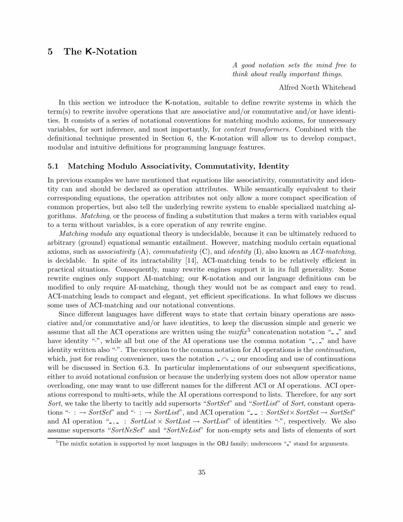
5 The K-Notation

A good notation sets the mind free tothink about really important things.

Alfred North Whitehead

In this section we introduce the K-notation, suitable to define rewrite systems in which theterm(s) to rewrite involve operations that are associative and/or commutative and/or have identi-ties. It consists of a series of notational conventions for matching modulo axioms, for unnecessaryvariables, for sort inference, and most importantly, for context transformers. Combined with thedefinitional technique presented in Section 6, the K-notation will allow us to develop compact,modular and intuitive definitions for programming language features.

5.1 Matching Modulo Associativity, Commutativity, Identity

In previous examples we have mentioned that equations like associativity, commutativity and iden-tity can and should be declared as operation attributes. While semantically equivalent to theircorresponding equations, the operation attributes not only allow a more compact specification ofcommon properties, but also tell the underlying rewrite system to enable specialized matching al-gorithms. Matching, or the process of finding a substitution that makes a term with variables equalto a term without variables, is a core operation of any rewrite engine.

Matching modulo any equational theory is undecidable, because it can be ultimately reduced toarbitrary (ground) equational semantic entailment. However, matching modulo certain equationalaxioms, such as associativity (A), commutativity (C), and identity (I), also known as ACI-matching,is decidable. In spite of its intractability [14], ACI-matching tends to be relatively efficient inpractical situations. Consequently, many rewrite engines support it in its full generality. Somerewrite engines only support AI-matching; our K-notation and our language definitions can bemodified to only require AI-matching, though they would not be as compact and easy to read.ACI-matching leads to compact and elegant, yet efficient specifications. In what follows we discusssome uses of ACI-matching and our notational conventions.

Since different languages have different ways to state that certain binary operations are asso-ciative and/or commutative and/or have identities, to keep the discussion simple and generic weassume that all the ACI operations are written using the mixfix 5 concatenation notation “ ” andhave identity “·”, while all but one of the AI operations use the comma notation “ , ” and haveidentity written also “·”. The exception to the comma notation for AI operations is the continuation,which, just for reading convenience, uses the notation � ; our encoding and use of continuationswill be discussed in Section 6.3. In particular implementations of our subsequent specifications,either to avoid notational confusion or because the underlying system does not allow operator nameoverloading, one may want to use different names for the different ACI or AI operations. ACI oper-ations correspond to multi-sets, while the AI operations correspond to lists. Therefore, for any sortSort, we take the liberty to tacitly add supersorts “SortSet” and “SortList” of Sort, constant opera-tions “· : → SortSet” and “· : → SortList”, and ACI operation “ : SortSet×SortSet→ SortSet”and AI operation “ , : SortList × SortList → SortList” of identities “·”, respectively. We alsoassume supersorts “SortNeSet” and “SortNeList” for non-empty sets and lists of elements of sort

5The mixfix notation is supported by most languages in the OBJ family; underscores “ ” stand for arguments.

35

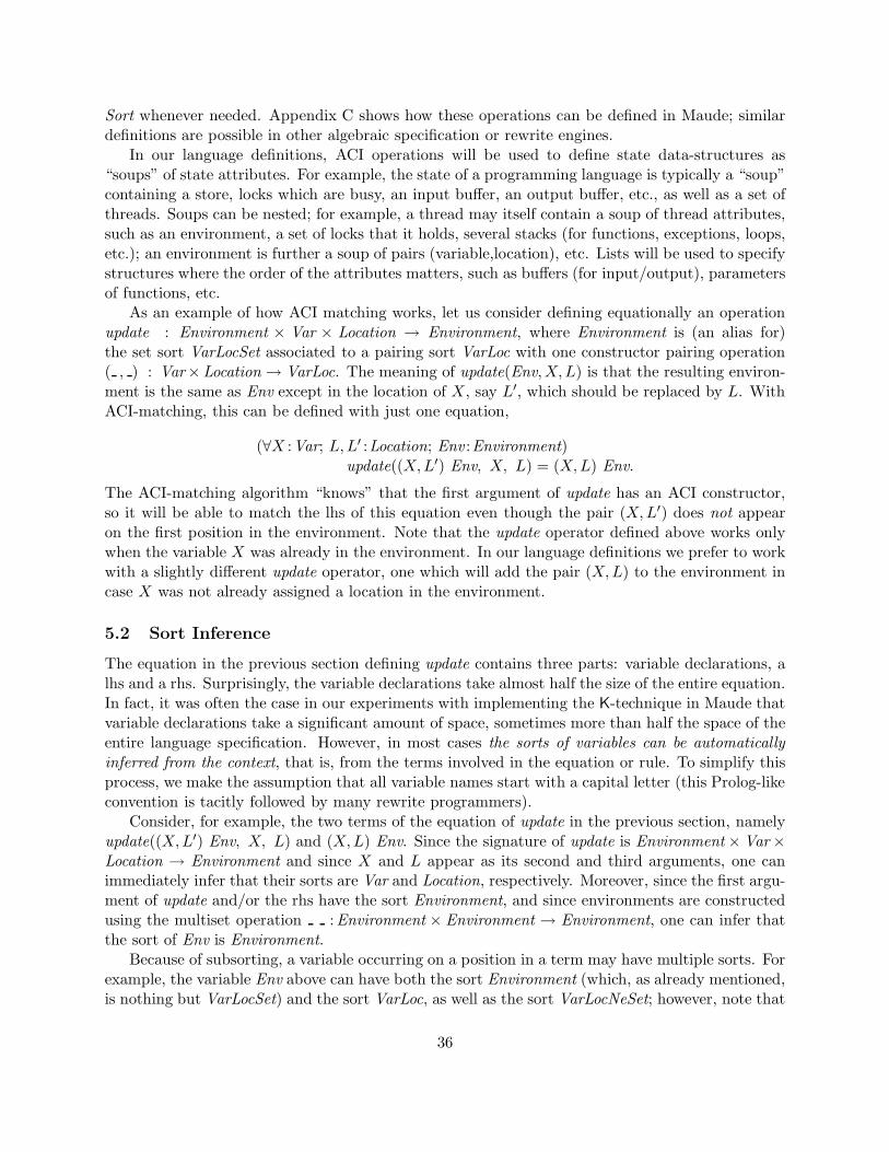
Sort whenever needed. Appendix C shows how these operations can be defined in Maude; similardefinitions are possible in other algebraic specification or rewrite engines.

In our language definitions, ACI operations will be used to define state data-structures as“soups” of state attributes. For example, the state of a programming language is typically a “soup”containing a store, locks which are busy, an input buffer, an output buffer, etc., as well as a set ofthreads. Soups can be nested; for example, a thread may itself contain a soup of thread attributes,such as an environment, a set of locks that it holds, several stacks (for functions, exceptions, loops,etc.); an environment is further a soup of pairs (variable,location), etc. Lists will be used to specifystructures where the order of the attributes matters, such as buffers (for input/output), parametersof functions, etc.

As an example of how ACI matching works, let us consider defining equationally an operationupdate : Environment × Var × Location → Environment, where Environment is (an alias for)the set sort VarLocSet associated to a pairing sort VarLoc with one constructor pairing operation( , ) : Var×Location → VarLoc. The meaning of update(Env,X,L) is that the resulting environ-ment is the same as Env except in the location of X, say L′, which should be replaced by L. WithACI-matching, this can be defined with just one equation,

(∀X :Var; L,L′ :Location; Env :Environment)update((X,L′) Env, X, L) = (X,L) Env.

The ACI-matching algorithm “knows” that the first argument of update has an ACI constructor,so it will be able to match the lhs of this equation even though the pair (X,L′) does not appearon the first position in the environment. Note that the update operator defined above works onlywhen the variable X was already in the environment. In our language definitions we prefer to workwith a slightly different update operator, one which will add the pair (X,L) to the environment incase X was not already assigned a location in the environment.

5.2 Sort Inference

The equation in the previous section defining update contains three parts: variable declarations, alhs and a rhs. Surprisingly, the variable declarations take almost half the size of the entire equation.In fact, it was often the case in our experiments with implementing the K-technique in Maude thatvariable declarations take a significant amount of space, sometimes more than half the space of theentire language specification. However, in most cases the sorts of variables can be automaticallyinferred from the context, that is, from the terms involved in the equation or rule. To simplify thisprocess, we make the assumption that all variable names start with a capital letter (this Prolog-likeconvention is tacitly followed by many rewrite programmers).

Consider, for example, the two terms of the equation of update in the previous section, namelyupdate((X,L′) Env, X, L) and (X,L) Env. Since the signature of update is Environment× Var×Location → Environment and since X and L appear as its second and third arguments, one canimmediately infer that their sorts are Var and Location, respectively. Moreover, since the first argu-ment of update and/or the rhs have the sort Environment, and since environments are constructedusing the multiset operation :Environment × Environment → Environment, one can infer thatthe sort of Env is Environment.

Because of subsorting, a variable occurring on a position in a term may have multiple sorts. Forexample, the variable Env above can have both the sort Environment (which, as already mentioned,is nothing but VarLocSet) and the sort VarLoc, as well as the sort VarLocNeSet; however, note that

36

there is only one largest sort among the three, namely Environment. If an occurrence of a variablecan have multiple sorts, we assume by default, or by convention, that that variable occurrence hasthe largest sort among those sorts that it can have. If there is no such largest sort then we assumevariable sorting to be “ambiguous”; if variable sorting is ambiguous for this reason, then most likelythe order-sorted signature has problems which would lead to ambiguous parsing anyway, so theseproblems would probably be flagged by the parser.

This “largest sort” convention corresponds to the intuition that we assume the “least” infor-mation about each variable occurrence; indeed, the more concrete the (sub)sort of a variable, the“more information” one has about that variable. If the same variable appears on multiple positionsthen we infer for that variable the “most concrete” sort that it can have among them. Technically,this is the intersection of all the inferred largest sorts on the different positions where the variableappears; if there is no such intersection sort then, again, we declare the sorting process of thatvariable ambiguous.

If the variable sort-inference process is ambiguous, or if one is not sure, or if one really wants adifferent sort than the inferred one, or even simply for clarity, one is given the possibility to sortterms, in particular variables, “on-the-fly”: we append the sort to the term or variable using “:”,e.g., t : Sort or Z : Sort. For example, from the term update(Env,X,L) one can only infer thatthe sort of Env is Environment, the most general possible under the circumstances. If for somereason (though we do not see any reason in this particular case) one wants to refer to a “special”environment of just one pair, then one can write update(Env :VarLoc,X,L).

Variable sort inference in the context of order sorted signatures is an interesting and challengingproblem, that we only partly address here. Also, syntactic criteria for non-ambiguous sort inferenceseem to be quite useful and non-trivial. The complexity of sort inference is yet another interestingand apparently non-trivial problem. We hope that all these problems will be addressed in the nearfuture, and that an efficient variable sorting algorithm will be implemented as part of a systemsupporting the K framework. For the time being we use sort inference just as a convenient wayto avoid writing long and heavy equations and rules. For now, the reader interested in defininglanguages using the K framework is expected to perform the sort inference process “in mind” todeduce the sorts of all the variables, and then to declare them appropriately in a rewrite system.The name of variables can also serve as a hint to the user. Indeed, there is not much doubt thatEnv has sort Environment, or that L has sort Location. One may even imagine a sorting conventionin which the root of a variable name (i.e., after dropping prime or digit suffixes) is a prefix of a sortname or its alias; we prefer to postpone this issue until an implementation of K takes shape.

5.3 Underscore Variables

With the sort inference conventions, the equation defining the operation update can therefore bewritten as

update((X,L′) Env, X, L) = (X,L) Env.

Note that the location L′ that occurs in the lhs is not needed; it is only used for “structural”purposes, i.e., it is there only to say that the variable X is allocated at some location, but wedo not care what that location is (because we change it anyway). Since this will be a commonphenomenon in our language definitions, we take the liberty to replace unnecessary letter variablesby underscores, like in Prolog. Therefore, the equation above can be written

update((X, ) Env, X, L) = (X,L) Env.

37

Let us consider a more complex and yet very common situation, namely (here only a fragmentof) the definition of variable lookup in a multi-threaded language. In our language definitions, manystate attribute “soups” will be wrapped with specific operators to keep them distinct from othersoups. For example, environments will be wrapped with an operation such as env : Environment→ThreadAttribute before they are placed in their threads’ state attribute soup; the threads’ state isfurther wrapped with an operation thread :ThreadAttributeSet → StateAttribute. Thus, with theunderscore conventions discussed in this section, if we want to find the location of a variable X inthe environment of a thread, then we match the thread against the term

thread(env((X,L) ) )

and find the desired location L (assume that X is already instantiated to some concrete programvariable); in this “pattern” term, the first underscore variable matches the rest of the environment,while the second matches the rest of the thread attributes (such as the resources that thread holds,its various stacks, its continuation, etc.).

5.4 Tuples

Like we need to pair variables and locations to create environments, we will often need to tuple twoor more terms in order to “save” current information for later processing. This is similar to “record”data-types in conventional programming languages. Most functional languages provide tuples ascore data-types. However, algebraic specification and rewriting logic do not have builtin tuples,so they need to be defined; their definition is, as expected, straightforward. To save space andincrease the readability of our language definitions, we avoid defining all these tupling operations.Like the sorts of variables, their arities can also be inferred from the context. Concretely, if theterm (X1 : Sort1, X2 : Sort2, . . . , Xn : Sortn) appears in some context (the variable sorts may beinferred from the remaining context using the techniques above), then we implicitly add to thesignature the sort Sort1Sort2...Sortn and the operation

( , , . . . , ) : Sort1 × Sort2 × · · · × Sortn→ Sort1Sort2...Sortn.

To keep the number of tupling operations small and to also avoid parsing conflicts, if two ormore tupling terms appear in a specification with the same number of arguments and the sorts ofthe arguments of one are larger than all the others, then only one tupling operation is added, theone for the larger sorts. In other words, if tuple terms (X1 :Sort1, X2 :Sort2, . . . , Xn :Sortn) and6

(X ′1 :Sort1’, X ′2 :Sort2’, . . . , X ′n :Sortn’) are encountered and Sort1’ < Sort1, Sort2’ < Sort2, ...,Sortn’ < Sortn, then only one operation is implicitly added to the signature, namely

( , , . . . , ) : Sort1 × Sort2 × · · · × Sortn→ Sort1Sort2...Sortn.

5.5 Contextual Notation for Equations and Rules

All the subsequent equations and rules will apply on just one (large) term, encoding the state of theprogram; note that our state is rather generous, containing everything needed to execute the entireprogram, including the program itself. Specifically, most of the equations and rules will apply on

6Recall that in order-sorted algebraic specification, “<” means “less than or equal to”; indeed, if s < s′ for sortss and s′, models in which the carriers of s and s′ are equal are also accepted.

38

subterms selected via matching, but only if the structure of the state permits it. In other words,most of our equations/rules will be of the form

C[t1] · · · [tn] = C[t′1] · · · [t′n] or C[t1] · · · [tn]⇒ C[t′1] · · · [t′n]

where C is some context term with n “holes” and t1, ..., tn are subterms that need to be replacedby t′1, ..., t′n in that context. Let us temporarily make no distinction between equations and rules;we will return to this important distinction shortly. The context C needs not match the entirestate, but nevertheless sometimes it can be quite large. To simplify notation and ease reading, weprefer to use the notation

C[t1t′1

] · · · [tnt′n

]

and call them all, generically, contextual rules. This notation follows a natural intuition: firstwrite the state context in which the transformation is intended to take place, then underline whatneeds to change, then write the changes under the lines. Our contextual notation above provesto be particularly useful when combined with the “ ” convention for variables: if “ ” appears in acontext C and it is not underlined, then it means that we do not care what is there (but we keepit unchanged).

As an example, let us consider the following common rule for variable lookup in the context ofa concurrent language (see also the second example in Section 5.3), already simplified using all thepreviously discussed notational conventions:

thread(k(X � K) env((X,L) Env) TS) store((L, V ) Store) ⇒thread(k(V � K) env((X,L) Env) TS) store((L, V ) Store).

The only difference between the two terms involved in the rule above is that the variable X atthe top of the continuation in the left term is replaced by V . The sorts of X, L, V and Env canbe readily inferred as discussed in Section 5.2. Also, the sort of Store and the sort of TS can beinferred similarly to the sort of Env; the sort of K, Continuation, can also be inferred similarly,noting that � is the list constructor for continuations (see Section 6.3). With the additionalconventions in this section, the rule above can be transformed into the following contextual rule,which avoids repeating state fragments and inventing names for variables that do not change (butneed to be there just to keep the above a well-formed rewrite rule):

thread(k(XV

� ) env((X,L) ) ) store((L, V ) ).

Our continuation-based language definitional technique, the K-technique proposed in the nextsection, makes the control/conditional context of a definition explicit as data context. A naturalconsequence of this definitional style is that the need for conditional rules almost disappears. Inthe very rare case that a condition is needed, then we use the expected notation:

C[t1t′1

] · · · [tnt′n

] ⇐ b

In our case studies on defining programming languages using K, we only needed very few con-ditional contextual rules. No conditional contextual rules were needed for most languages, some

39

of them relatively complex. This should not appear to be surprising, though: [25] shows how acontinuation-passing-style transformation applied automatically to a confluent conditional rewritesystem7 can systematically eliminate all the conditional rules by replacing them with computa-tionally equivalent unconditional ones. The conditions that we needed were all trivial booleanconditions, so we do not bother here to introduce notation for various types of conditions of equa-tions or rules in rewriting logic, such as equations, memberships, rules, shortcuts, matching inconditions, etc.

5.6 Structural, Computational and Non-Deterministic Contextual Rules

Let us now return to the important distinction between equations and rules in rewriting logic, anddiscuss how we accommodate it in our notation. A careful analysis of several languages that wedefined as rewrite logic theories led us to the conclusion that, in fact, one wants to distinguishamong three kinds of contextual rules, not only between two (as rewriting logic would suggest byits distinction between equations and rules):

• Structural, or non-computational. These are rules whose only role is to allow modificationsof the structure of the state, so that other contextual rules that have computational meaningcan apply. For example, the contextual rules that transform a program into a continuationterm, or the rules for creating the initial state, are all structural, their role being to “prepare”the expression for evaluation. These structural rules have absolutely no computational mean-ing. Intuitively, if one thinks of a programming language definition as a means to generate“computations” (i.e., sequences of execution steps) from programs, making complete abstrac-tion of state or syntax representation, then the structural rules are intended to generate noexecution steps in computations. Even though these rules may be executed by rewriting aswell by most rewrite engines, their corresponding rewrite steps are not visible as part of thecomputation, in a similar way that equations in executions of rewrite logic specifications arenot visible as transition steps in models. We can think of structural contextual rules as rules“modulo” which computations take place. We will use the following notation for these rules

C[t1t′1

] · · · [tnt′n

],

whose lines underlying subterms that change are dotted, signifying that these rules are“lighter” than the other rules whose lines are full. As expected, when K is translated intorewriting logic, structural contextual rules always translate into equations. Also, all the setand list implicit associativity and commutativity equations are structural, having no compu-tational meaning either.

• Computational. These are all the other contextual rules; we use the notation

C[t1t′1

] · · · [tnt′n

]

for them, where the lines underlying subterms that change are full. Each of these rulescaptures precisely one intended execution step of the program. When we translate K into

7Definitions of non-concurrent non-deterministic languages are expected to be indeed confluent.

40

rewriting logic, depending on the desired abstraction and the purpose of the translation,these computational rules can be translated either into equations or into rewrite rules. Ifthe language is sequential and deterministic and if one’s interest is in capturing an algebraicdenotational semantics of it (an initial algebra semantics where the denotation of each termis the value that it evaluates to), then all these computational rules can be translated intoequations. If one’s interest is in precisely capturing a dynamic semantics of the languagethat reflects all the computation steps that take place during any execution, then one shouldtranslate all the computational contextual rules into rewrite rules. While this appears tosemantically be the most appropriate choice, it may not always be practical, because theresulting executions may be too detailed. For example, if for certain common analysis pur-poses, such as model checking of concurrent programs, one is deliberately not interested insteps that do not change the concurrent behavior of a program, such as initializations offunction arguments, or break/continue of loops, or throwing exceptions, etc., then one cantranslate their corresponding contextual rules into equations. Recall that the initial modelof a rewrite theory collapses all states that are provably equal by equational reasoning, so asignificant state-space reduction can result as a consequence of such equational abstractions;experiments confirm this fact.

• Non-deterministic. Non-deterministic rules are always a (typically quite small) subset of thecomputational rules. To distinguish them from the other computational rules, we box them:

C[t1t′1

] · · · [tnt′n

]

These are rules that can potentially change the deterministic behavior of a program. If a lan-guage is sequential and deterministic, then there is no need to declare any of the contextualrules non-deterministic, because the rules are expected to be Church-Rosser on the termsof interest8 (well-formed programs) if the programming language is correctly defined. Forexample, a simple calculator language that only evaluates side-effect-free expressions is deter-ministic, even though several rules may possibly apply concurrently and non-deterministicallyduring evaluation tasks; what is important is that the final result of an evaluation does notdepend on the order in which or the places where these rules apply. However, if a languageadmits concurrency, then some rules may lead to non-deterministic behaviors; for example,reads and writes of memory locations, or acquire and release of locks can lead to differentbehaviors of concurrent programs. Technically, a rule is non-deterministic when there areterms of interest (well-formed programs or fragments of programs) on which two rule in-stances (possibly of the same rule) can be applied at the same time, at least one of thembeing an instance of our rule, and depending upon which of the two rules is chosen first onegets different behaviors of the program. If an instance of a rule can be swapped with anyother rule instance at any moment, then the former rule is obviously not non-deterministic.Intuitively, one can think of the non-deterministic rules as those rules that show the relevant

8The contextual rules defining a programming language are not Church-Rosser in the strict sense of the termin general, even though the language is sequential. Indeed, one can imagine a term containing two continuationstructures, both with the next task to write the same variable; depending upon which rule is picked first, one canobtain totally different normal forms. However, such a term will never appear during the evaluation of a well-formedsequential program (though one would need to prove that), so we say that such terms are not of interest.

41

execution steps in the execution of a concurrent program, namely those where the behaviorof the program can possibly change if another choice is being made. We call deterministic allthe rules which are not non-deterministic (these include also the structural rules).

The structural and computational declarations of contextual rules are modular, in the sensethat one does not need knowledge about the entire language in order to declare a rule structuralor computational. However, the non-deterministic declaration of rules is trickier and needs globalinformation about the program. For example, one cannot know when one defines a variable lookuprule whether the defined language is concurrent or not; if it is, then that rule needs to be declarednon-deterministic. Also, it is impossible to identify the non-deterministic rules automatically ingeneral, because this problem is harder than testing confluence, a notorious undecidable problem.

The non-deterministic rule declarations should be regarded as annotations, rather than as a corepart, of the semantics of a language, telling the designer that those rules, and only those, may non-deterministically change the behavior of the program. This information can be very precious forcertain analysis purposes, such as model checking. Indeed, since the other computational rules areimplicitly declared to not affect the overall behavior of the concurrent program, a model checker forthe defined language can regard their transitive application as atomic, thus reducing significantlythe state space that needs to be analyzed: only the instances of the non-deterministic rules canlead to increases in the number of states of the system that need to be analyzed. In terms ofmodel checking, the deterministic rules can be regarded as atomic abstractions (also related topartial-order reduction) and their instances can therefore be grouped and applied together in one“big” atomic step, without worrying about missing any behavior of the concurrent program. Theintuition underlying the distinction between non-deterministic and deterministic contextual rulesclosely resembles the distinction between rules and equations in rewriting logic; indeed, when wetranslate K language definitions into rewriting logic for program analysis purposes, we translatethe non-deterministic ones into rewrite rules and the deterministic ones into equations.

5.7 Matching Prefixes, Suffixes and Fragments

We here introduce another important piece of notation, which will help us further compact lan-guage definitions by eliminating the need to mention unnecessary underscore variables. Recall the“pattern” term thread(env((X,L) ) ), useful for variable lookup, that we discussed in Section 5.3.The two underscores in this pattern term make the pattern look heavier and harder to read thanneeded. Conceptually they bring nothing new: they are there just for formal reasons, to writeterms using a mathematically rigorous notation. What one really wants to say here is that one isinterested in the pair (X,L) that appears somewhere in the environment that appears somewherein the thread. In any domain, good notation is meant to have a low, hopefully close to zero rep-resentational distance to the concepts that it refers to. In our particular domain of programminglanguages, we believe, admittedly subjectively, that the notation thread〈env〈(X,L)〉〉 for the samepattern term is better than the one using the underscores. We next formalize our notation.

By convention, whenever “ ◦ ” is an ACI or AI operator constructing a term that appears insome context, say C�, we write

• C(T 〉 (i.e., left parenthesis right angle) as syntactic sugar for C(T ◦ ),

• C〈T ) (i.e., left angle right parenthesis) as syntactic sugar for C( ◦ T ),

42

• C〈T 〉 (i.e., left and right angles) as syntactic sugar for C( ◦ T ◦ ).

If “ ◦ ” is an ACI operator then the three notations above have the same effect, namely that ofmatching T (which can be itself a set of several attributes) inside the soup in the hole of contextC; for simplicity, in this case we just use the third notation, C〈T 〉. The intuition for this notationcomes from the fact that the left and the right angles can be regarded as some hybrid betweencorresponding “directions” and parentheses. For example, if “ ◦ ” is AI (not C) then (T 〉 can bethought of as a list starting with T (the left parenthesis) and potentially continuing to the right(the right angle); in other words, it says that T is the prefix of the list in the hole of C. Similarly,〈T ) says that T is a suffix of and 〈T 〉 says that T is a contiguous fragment of the list in the holeof the context C. If “ ◦ ” is also commutative, i.e., an ACI operator, then the notions of prefix,suffix and fragment are equivalent, all saying that T is a subset of the set at the hole of C.

This notational convention will be particularly useful in combination with other conventionspart of the K notation. For example, the input and output of the programming language definedin the sequel will be modeled as comma separated lists of integers, using an AI binary operation“ , ” of identity “·”; then in order to read (consume) the next two integers I1, I2 from the inputbuffer, or to output (produce) integers I1, I2 to the output buffer, all one needs to do (as part of alarger context that we do not mention here) is:

in(I1, I2

·〉 and, respectively, out〈 ·

I1, I2

)

The first matches the first two integers in the buffer and removes them (the “·” underneath theline; recall that “·” is by convention the unit, or the identity of all ACI or AI operators), whilethe second matches the end of the buffer (the “·” above the line) and appends the two integersthere. Note that the later works because of the matching modulo identity: out〈·) is a shorthandfor out( , ·), where the underscore matches the entire list; replacing “·” by the list I1, I2 is nothingbut appending the two integers to the end of the list wrapped by out (thanks to the AI attributesof the comma operator).

As another interesting example, this time using an ACI operator, consider changing the locationof a variable X in the environment of a thread to another location, say L (in order for such adefinition to make sense, one should make sure that there is enough context in order for L to beproperly instantiated); this could be necessary in the definition of a language allowing declarationsof local variables, when a variable with the same name, X, is declared locally and thus “shadows”a previously declared variable with the same name. This can be done as follows (part of a largercontext):

thread〈env〈(X,

L

)〉〉.

We take the liberty to use the “angle” notation above also in situations where the correspondingsoups are not necessarily “wrapped” by specific attributes, but only when, by using all the sortand tuple operation inference conventions above, such a use does not lead to any confusion. Forexample, as part of the semantics of most programming languages, we need to evaluate lists ofexpressions sequentially. To achieve this elegantly, we will just place the list of expressions on thetop of the continuation and “wait” for it to be transformed into a list of corresponding values.As part of this process, we use an auxiliary operator pairing a list of expressions and a list of

43

values, and then evaluate the expressions one by one, moving their corresponding values (as theyare generated) at the end of the list of values. The following is the contextual rule that picks thenext expression and places it on the top of the continuation for evaluation:

k( ·E

� ((E :Exp·〉, :ValList)〉

The “·” on the top of the continuation is generated by the matching modulo identity; by replacingit with the expression E, we are saying that we place E at the top of the continuation. Fromthe sorting information present in the second continuation item, it becomes clear that that itemcorresponds to the pairing operation of ExpList and ValList; since its first argument is undoubtedlya list of expressions, we use the angle-bracket convention to identify the first expression in the list,E, and then remove it by replacing it with the “·”. All the contextual rules for this common taskof evaluating lists of expressions are part of the core of K and will be discussed in detail in Section6. Note that the rule above is structural, because it carries no computational meaning.

5.8 Structural Operations

We next introduce the most subtle of our notational conventions, which plays a crucial role inincreasing the modularity of programming language definitions. This notational convention isbased on the observation that, in programming language definitions, it is always the case that thestate of the program, a term in our representation, does not change its significant structure duringthe execution of the program. For example, the store will always stay at the same level in the statestructure, typically at the top level, and the environments will be declared as part of each thread’ssoup and will stay there during the execution. If certain state infrastructure is known to stayunchanged during the evaluation of any program, and if one is interested in certain attributes thatcan be unambiguously located in that state infrastructure, then we are going to take the libertyto only mention those attributes as part of the context assuming that the remaining part of thecontext can be generated automatically (statically).

To make this intuition clearer, let us first consider an artificial example. Suppose that attributesa1 and a2 wrap ACI soups and that their concrete positions in the state structure can be inferredunambiguously (we will see shortly how). Suppose also that one is interested in changing subtermst1 (to t′1) and t2 (to t′2) that are part of the soups wrapped by attributes a1 and a2. Then onewould like to write this contextual rule simply as:

a1〈t1t′1〉 a2〈t2

t′2〉

With the current notational conventions, this rule would parse only if a1 and a2 lay together withinthe same soup. However, due to various reasons, the two attributes may be located at differentlevels in the state. For example, a1 and a2 may be part of the soups of other attributes, say b1 andb2, respectively, in which case one is expected to write the rule above as

b1〈a1〈t1t′1〉〉 b2〈a2〈t2

t′2〉〉

The second rule above is not only unnecessarily more complicated and harder to read than thefirst one (since the places of a1 and a2, i.e., inside the soups wrapped by b1 and b2, are known, then

44

why mention them again?), but also suffers from being more rigid than the first. Indeed, if for anyreason one decides to change the structure of the state and move the attributes a1 and a2 to otherplaces in the state (still keeping their unique identity), then one would also need to transform thesecond rule accordingly; note, however, that one would not need to change the first rule.

Such changes of state structure are quite common in language definitions. For example, onemay consider different state structures for sequential languages than for concurrent ones. Indeed,in a concurrent language one may want the various threads to each wrap their own state (environ-ment, locks, control structures, etc.) for clarity and to avoid confusion among attributes with thesame name associated with different threads, while in a sequential language that is not necessarybecause there is only one thread, so the content of that thread, including its environment andcontrol structures, can be moved to the top level of the state. This way, rules defined for the con-current language involving both thread attributes (e.g., environments) and other attributes (e.g.,the store), are not well-formed anymore as are: these need to be modified to account for the newstate structure, thus breaking the encapsulation principle of the definitions of language features inparticular and the modularity of programming language definitions in general.

thread

busy

527…

3,8,2,5,6,9,0in

3,6,7,8,9,1out

17

nextLoc

(L1, V1)(L2, V2)

(Ln, Vn)

…

store

…

controlfstack xstack lstack(X1, L1)

(X2, L2)…

env holds

(5, 3)(7,1)

…

thread

1

… …

k

controlfstack xstack lstack(X1, L1)

(X2, L2)…

env holds

(1, 4)(2,0)

…

k

Figure 5: FUN state infrastructure.

The state structure which is not intended to change can be, fortunately, specified very easilyby just “marking” certain operations as structural. Consider, for example, a state instance like theone in Figure 5 of the programming language FUN that we will define in the next sections. Ascan be seen, the state is a nested soup of ingredients, or attributes: the store wraps a set of pairs(location,value) and is located at the top level in the state together with input/output buffers, aset of busy locks, a next free location, as well as one attribute per thread (added dynamically);each thread contains a soup of its attributes (that’s why we use the term “nested soup”), suchas continuation, an environment, a set of locks it holds, as well as its control information; thecontrol information is itself a soup whose ingredients are the various stacks needed to encode thecontrol context of the program (for functions, loops, exceptions, etc.). Most of the operations that

45

are constructors for states are structural, i.e., give the state a structure which does not changeas the programs are executed. In our example language, the following top level state constructoroperations can be declared as structural:

Structural operationsthread : ThreadState → StateAttribute [�]busy : IntSet→ StateAttributein : IntList→ StateAttributeout : IntList→ StateAttributestore : LocValSet→ StateAttributenextLoc : Nat→ StateAttribute

The star “�” attribute of thread means that that attribute can have multiple occurrences in thestate, all at the same level; this notation will be discussed shortly. Here we assumed that other basicsorts and operations are already declared, such as those for locations, values, integers, naturals,etc. Also, following our previous notational conventions, we assume that sets and lists of such basicsorts exist whenever we need them. The state of the programming language is nothing but a setof state attributes, i.e., of terms of sort StateAttribute. Indeed, we take the liberty to use the sortState as a more intuitive “alias” for StateAttributeSet. At this moment, we define and use sortaliasing informally; introducing a formal notation for sort aliasing is not difficult, but we prefer topostpone it until we implement K. Further, constructor operators for thread states can, and shouldalso be declared as structural. We declare a sort ThreadAttribute and, as before, take the libertyto alias the sort ThreadAttributeSet by the more intuitive sort name ThreadState:

Structural operationsk : Continuation→ ThreadAttributeenv : Environment→ ThreadAttributecontrol : Control → ThreadAttributeholds : IntIntSet→ ThreadAttribute

In the above operation declarations, we used the sort Continuation as an alias for ContinuationItem-List, Environment as an alias for the sort VarLocSet and Control as an alias for ControlAttributeSet ;we may also use Ctrl as an alias sort for Control.

The control of a thread is also a soup of various control attributes, which should be declared asstructural operations as well:

Structural operationsfstack : FunctionStack→ ControlAttributexstack : ExceptionStack→ ControlAttributelstack : LoopStack → ControlAttribute

The sorts FunctionStack, ExceptionStack and LoopStack alias various list sorts which we do notneed here but will explain in the next section.

The structural operations above form a tree whose edges are the structural operations andwhose nodes are the largest sorts that are supersorts of the result sort of each structural operation,like in Figure 6. For example, the target node of the edge control is ThreadState, which aliases thesort ThreadAttributeSet ; that is because the target sort of the operation control was declared to be

46

ThreadAttribute and its largest supersort is ThreadAttributeSet. Note that, in general, the structuraloperations may yield a multi-graph whose multi-edges correspond to the structural operations;that is because operations may have more than one argument and because one may have cycles inoperation declarations. However, for simplicity, in this paper we assume that structural operationsare defined in such a way that their corresponding multi-graph is a tree; we believe, however,that our notational conventions can be extended to general multi-graphs (but we are currently notmotivated to do it).

CtrlContinuation

FunctionStack ExceptionStack LoopStack

k

fstack xstack lstack

Environment= VarLocSet

IntListIntList Nat

env control

LocValSet

State

outin storenextLoc

ThreadState

IntIntSet

holds

IntSet

busythread *

Figure 6: FUN state structural operations.

5.9 Context Transformers

We are now ready to introduce our notational convention for context transformers. Assuming thatthe various structural operations have unique names, or in other words that their correspondingtree has unique labels on its edges, then one can use the structural tree to automatically transformpartial, possibly non-well-formed contexts into concrete ones that are well-formed within the currentstructure of the state. These context transformers are applied statically, before the rewrite systemis executed. Suppose, for example, that in order to define a particular language feature, such asprinting a value, one is interested only in the continuation (k) of a thread (the continuation tellswhat is the next task to perform, in this case printing of some value) and the output buffer (out).In spite of the fact that these two attributes are located at different levels in the state nested soup,thanks to the context transformer notational convention one is allowed to write contextual rules asif they are at the same level, that is, of the form:

k(...) out(...)

Here we do not care about the particular terms that are wrapped by the attributes (the “...”),nor whether they are replaced by some other terms or not. Complete details will be given in the

47

next section. We are only interested in the structure of the state context in which the attributesmentioned in the partial contextual rule make sense. For example, by examining the tree associatedto the state structural operations in Figure 6, one can easily see that the only way to complete thepartial context above is to mention the entire path to the attribute k, that is:

thread〈k(...)〉 out(...)

To properly transform the context, one may need to add artificial variables corresponding to non-interesting branches at each node in the tree. By convention, we only use the special underscore “ ”variables for this task; combined with the left and right angle convention to eliminate unnecessaryunderscore variables, we get the concrete contextual rule above.

Let us now consider a more complex example, corresponding to retrieving the value associatedto some program variable. In order to find the value corresponding to a variable that appears asthe next task in the continuation k, one needs to retrieve the location associated to that variablefrom the environment env and then the value associated with that location in the store. Ignoringagain the non-structural details, thanks to the context transformer convention one can simply writethis contextual rule as follows:

k(...) env(...) store(...)

By examining the unique way in which these attributes make sense together, this partial contextualrule can be automatically transformed into:

thread〈k(...) env(...)〉 store(...)

A subtle aspect of the context transformation above is that both k and env attributes are partof each thread. Since there can be many threads running concurrently in a program, how canone know that one did not mean the k attribute of one thread and the env attribute of anotherthread in the partial contextual rule above? The simple answer to this concern is the following:the context transformers are applied statically, based on just the structural information providedby the syntactic definition of the structural operators. The fact that there can be several threadsat the same time part of the top-level state soup is a purely semantic issue, consequence of theother contextual rules defining the language under consideration. There can be language definitionswhere the state may contain more than one store (for example a distributed language) during theevaluation of the program. However, once the store and the operations on the path to it in the statewere declared as structural and the tree associated to the structural operations is unambiguous,there is only one way to complete/transform any partial context referring to the store.

Then what if, for some reason which may not make sense for our particular language but couldmake sense for other languages, one really means the k of one thread and the env or another thread?In such a case one is supposed to give the context transformation procedure more information,namely to mention explicitly the two threads:

thread〈k(...)〉 thread〈env(...)〉 store(...)

Another interesting situation which can appear in some language definitions is when one wantsto refer to two attributes with the same name in a contextual rule. In the language defined in thispaper thread communication is via shared memory and locks, but in some languages one may wantto synchronize threads using a wait/notify mechanism and one may want to define this by matching

48

both the notifying thread and the waiting one, in which case one would end with two attributes withthe same name in some contextual rules (thread in this case). Since attribute names are distinctin the structural operations’ tree, an attribute operation, say a, can appear multiple times in acontextual rule only if some attribute on the path from the root of the tree to a appears multipletimes in its corresponding attribute set; this attribute can be either a or some other attribute at ahigher level.

From practical considerations and our experience with using the K notation, we believe thata language designer typically knows in advance which attributes are allowed to appear multipletimes in their soup. For example, if one designs a multi-threaded language, one knows that theattribute thread can appear multiple times in the soup of threads, because threads are intended tobe created and terminated dynamically. However, one also knows that environments, for example,are not intended to appear multiple times within one thread. In principle, a careful analysis ofa complete language definition would allow one to deduce which attributes should be allowed toappear multiple times and which should not; for example, one can see that there are rules whichadd one more thread to the state, while there are no rules that add an environment to an existingthread state. However, we prefer not to infer this important structural information automaticallyfrom the way the contextual rules are written for two reasons:

• first, because it is meaningful and useful for a language designer to be aware and explicitlystate which attributes are allowed to multiply; and

• second, because an automation of this process seems non-trivial to implement.

Since attributes that multiply are by far less frequent that attributes which do not multiply, weintroduce a notation in K for those which multiply: we put a star “�” on the arrow labeled withthose attributes in the state attributes’ tree; see, for example, the star on the thread attribute inFigure 6. With this convention, it is now easy to disambiguate contextual rules. In particular, thepartial contextual rule

k(...) k(...)

would be completed tothread〈k(...)〉 thread〈k(...)〉

rather than tothread〈k(...) k(...)〉.

If some contextual rules cannot be transformed with this convention then, at this moment, we saythat the specification is ambiguous or faulty.

It is fair to mention it here again that the K notation proposed in this section and intensivelyused in the next is not yet supported by any mechanical system, tool or prototype. We are only usingit by hand to define languages compactly and modularly on paper. However, it is a straightforwardexercise to transform a definition of a language using the K notation into a rewrite logic specificationthat can be executed on existing systems. For example, it took a graduate student (Traian FlorinSerbanuta, who is also currently implementing a parser and a mechanical translation of K intorewriting logic) little time to hand translate into Maude the K-definition of FUN discussed next(Appendixes F and G show the Maude definitions of both sequential and concurrent FUN).

In our current programming language definitions we regard context transformers as well asthe translation of all the other notational conventions as a pre-compilation step of our language

49

definitions, which can only be performed once the structural operators are completely defined. Themodularity of our language definitions comes from the fact that the same definition of a particularlanguage feature pre-compiles differently under different state structures. As an example, in severalof our language definitions we were faced with the controversial issue of whether the continuationof a thread should really be at the same level with the control and the environment, letting thecontrol structure maintain only the execution stacks, or it should instead be part of the control ofthat thread. Fortunately, with the K notation it essentially does not matter whether k is definedas part of the control of threads or at the same level with it. If one wants the former, all one needsto do is to replace the operation declaration

k : Continuation→ ThreadAttribute

with the declarationk : Continuation→ ControlAttribute

Nothing else needs to be changed (but the entire language definition needs to be pre-compiledagain). As with the other notational conventions, one will become more familiar with the contexttransformers as one defines concrete languages. The next section shows a middle-complexity casestudy.

50

6 The K-Technique: Defining the FUN Language

We exemplify our K-technique by defining a simple, yet non-trivial programming language calledFUN, which contains higher-order functions with return, let and letrec, lists, sequential composition,assignments, loops with break and continue, input/output, parametric exceptions, callcc and con-currency via threads and synchronization. We assume the reader familiar with these programminglanguage features. In this section we define all features except callcc and concurrency, as part of asublanguage that we call “sequential FUN”; we complete the definition of FUN in the next section,where we define callcc and concurrency as language extensions, to reflect the modularity of our def-initional framework. Our main goal is to focus on FUN’s semantics, so we just pick some familiarsyntax and assume an existing parser. Depending upon the rewriting engine one uses to formalizeit, one can use the definition below as is to execute and to analyze (BFS reachability and/or LTLmodel checking) FUN programs. The complete K-definition of sequential FUN is shown in Figure 7,and a Maude-ified version of it in Appendix F. Figure 9 shows how the language can be extendedwith callcc and concurrency, and Appendix G a complete Maude-ified definition.

6.1 Syntax

FUN is an expression language. Expressions may evaluate to values of different types. We define thesyntax of FUN as an order-sorted algebraic signature using the mixfix notation. It is known that themixfix notation is equivalent to the more common (but slightly harder to relate to term rewriting)BNF notation, by interpreting each sort into a non-terminal and each operation as a production.If underscores are not explicitly mentioned in an operation’s name then that operation is assumedin prefix notation. We assume already existing definitions of integers and identifiers, coming withsorts Int and Var, respectively. One can either use builtins or define these. We therefore introduceone sort Exp with Int < Exp and Var < Exp, and define the following operations:

true, false, skip : → Exp+ , − , ∗ , / , ..., ≤ , ≥ , ..., ∧ , ∨ , ... : Exp× Exp→ Exp

if then : Exp× Exp→ Expif then else : Exp× Exp× Exp→ Expfun → : VarList× Exp→ Exp( ) : Exp× ExpList→ Exp

return : Exp→ Explet, letrec : VarList× ExpList × Exp→ Exp; : Exp× Exp→ Exp

[ ] : ExpList→ Expcar, cdr, null? : Exp→ Expcons : Exp× Exp→ Exp:= : Var× Exp→ Exp

read() : → Expprint : Exp→ Exptry catch( ) :Exp×Var× Exp→ Expthrow : Exp→ Expwhile( ) : Exp× Exp→ Exp

51

import BOOL, INT, REAL, K-BASIC

Structural operations

CtrlContinuation

FunctionStack ExceptionStack LoopStack

k

fstack xstack lstack

Environment= VarLocSet IntListIntList Nat

env control

LocValSet

State

outin store

nextLoc

eval :Exp × IntList→ IntListresult : State→ IntList

ff. . . .

8>>>><>>>>:

eval(E, Il)result(k(E) env(·) control(fstack(·) xstack(·) lstack(·)) in(Il) out(·) store(·) nextLoc(0))

result〈k( : Val) out(Il)〉Il

Var, Bool, Int, Real < ExpBool, Int, Real < Val

ff. . . . . . . . . . . . . . . . . . . . . . . . . . . . . . . . . . . . . . . . . . . . . . . . . . . . . . . . . . .

jk(X

V〉 env〈(X, L)〉 store〈(L, V )〉

not : Exp→ Exp [!, notBool : Bool → Bool ]+ :Exp× Exp→ Exp [!, +Int : Int× Int→ Int, +Real :Real ×Real→ Real]≤ : Exp × Exp→ Exp [!, ≤Int : Int× Int→ Bool, ≤Real : Real× Real→ Bool]

skip :→ Exp [unit :→ Val]

if then : Exp× Exp→ Expif then else : Exp× Exp× Exp→ Exp [!(1)[if]]

ff. . .

jif B then E

if B then E else skipbool (true) � if(E1, E2)

E1

bool(false) � if(E1, E2)E2

fun → :VarList× Exp→ Exp( ) :

Exp× ExpList→ Exp [![app]]return : Exp→ Exp [!]closure :VarList× Exp × Set[Var � Loc]→ Val

popFstack :→ ContinuationItem

9>>>>>>>>=>>>>>>>>;

.

8>>>>>>>>>><>>>>>>>>>>:

k( fun Xl→ Eclosure(Xl, E,Env)

〉 env(Env)

(k((closure(Xl, E,Env), Vl) � app � KVl � bind(Xl) � E � popFstack

) fstack( ·(K, Env′, C)

〉 C :Ctrl) env(Env′Env

)

k( :Val � popFstackK

) fstack((K, Env, )·

〉 env(Env

)

(k( :Val � return �

K) fstack((K, Env, C)

·〉 :Ctrl

C) env(

Env)

let, letrec :VarList×ExpList×Exp→Exp

ff. . .

jk( let(Xl, El, E)

El�bind(Xl)�E�Env〉env(Env) k( letrec(Xl,El, E)

bind(Xl)�El�write(Xl)�E�Env〉env(Env)

; : Exp× Exp→ Exp [!]:= : Var× Exp→ Exp

ff. . . . . . . . . . . . . . . . . . . . . . . . . . . . . . . . . . . . . . . . . . .

j(V1 : Val·

, V2 : Val) � ;·

X := EE � write(X) � unit

[ ] : ExpList→ Exp [!, [ ] : ValList→ Val]

car, cdr, null? : Exp→ Exp [!]cons : Exp× Exp→ Exp [!]

9=; . . . . . . . . . . . . . . . . . . . . .

8>><>>:

[V :Val, ] � carV

[ :Val,Vl] � cdrVl

[·] � null?bool(true)

[ :Val, ] � null?bool(false)

(V, [Vl]) � cons[V,Vl]

read() : → Exp

print : Exp→ Exp [!]

ff. . . . . . . . . . . . . . . . . . . . . . . . . . . . . . . . . . . . . . . . . . . . . . . . . . . . .

jk(read()

int(I)〉 in(I

·〉 k(int(I) � print

unit〉 out〈 ·

I)

try catch( ) :

Exp× Var× Exp→ Expthrow : Exp→ Exp [!]

9=; . . . . . . . . .

8>>>>>><>>>>>>:

(k(try E′ catch(X) E � KE′

� popXstack) xstack( ·

(X, E,Env, K, C)〉 C :Ctrl) env(Env)

k( :Val � popXstackK

) xstack(( , , , K, )·

〉

(k( :Val � throw �

bind(X) � E � Env � K) xstack((X, E,Env, K, C)

·〉 :Ctrl

C) env(

Env)

while( ) :Exp×Exp→ Exp

for( ; ; ) :

Exp×Exp×Exp×Exp→ Expbreak : → Expcontinue : → Exp� :→ ContinuationItem

9>>>>>>=>>>>>>;

. . . . .

8>>>>>>>>>>>>>><>>>>>>>>>>>>>>:

while(B) E

for(skip;B; skip) E(k(for(S; B; J) E � K

S;B � �) lstack( ·

(B,E, J, Env, K, C)〉 C :Ctrl) env(Env)

k(bool(false) � �unit � K

) lstack(( , , , , K, )·

〉 k(bool(true)E; J;B

� �) lstack((B,E, J, , , )〉

(k(break �

unit � K) lstack(( , , ,Env, K,C)

·〉 :Ctrl

C) env(

Env)

(k(continue �

J;B � �) lstack((B, , J, Env, , C)〉 :Ctrl

C) env(

Env)

Figure 7: K definition of sequential FUN

52

for( ; ; ) : Exp× Exp× Exp× Exp→ Expbreak, continue : → Exp

In Section 8 we extend the syntax above with callcc and with threads and synchronization.

6.2 State Infrastructure

The picture at the top of Figure 7 shows the structural operators of sequential FUN. The structureof the state of the language will change when we add threads, as shown in Figure 9; Figure 5 showsan instance of the state of concurrent FUN. For all our language definitions in K, the state of thelanguage is a soup of attributes, each potentially comprising other soups of attributes. The par-ticular sort names that one chooses for the various soup ingredients are not technically important,though they can help users read and understand language definitions more easily. If the modularityof the language definition is one’s concern, then one can define the various soup ingredients “on-the-fly”, as the language features using them are introduced to the language. Modularity of ourdefinitional framework will be discussed in the next section, together with a detailed comparisonto Modular SOS [21]. Let us next discuss the various state attributes of sequential FUN, whoseprograms contain only one, implicit execution thread; all these attributes will be reused in thedefinition of concurrent FUN, with the same meaning.

One of the distinguished state attributes that appear in all our definitions in K is the continua-tion, which is wrapped using the attribute name k and which encodes the remaining computationtasks; our encoding and use of continuations is discussed in Section 6.3. The env attribute wrapsa set of pairs (variable, location), and the store attribute wraps a set of pairs (location,value). Lo-cations can be any structures, e.g., wrapped natural numbers such as location(7), providing a nextlocation operation: if L is some location, then next(L) is the “next” location, where the orderingis left uninterpreted. We assume the existence of environment and store update operations; forexample, for stores we assume that Store[L← V ] updates the value at location L in Store to V ; ifL is not in the store yet, then it adds the pair (L, V ) to Store. The state attribute nextLoc wrapsthe next available location. Note that FUN implementations/compilers can interpret locations andthe next operation many different ways, in particular as needed by an underlying garbage collector.

The attributes in and out contain the input and the output buffers (lists of integers) needed todefine the read() and print statements. Because of the various control-intensive statements of FUN,the control attribute contains itself several other attributes which are stacks that will store, intotuples, information needed to define the different control-intensive statements: fstack for functionswith return, xstack for exceptions, and lstack for loops with break and continue.

6.3 Continuations

There are many different ways to formally represent or define continuations; these are ultimatelyall equivalent and capture the same idea: a continuation encodes the remaining of the computation[23, 26]. More precisely, a continuation, say K, is a structure which, when passed a value, sayV , which can be thought of as the value of some local computation, “knows” how to finish theentire computation. One can use various notations for continuation invocation, such as “K(V )”, or“K V ”, or even “V � K” or “V � K”, or any other meaningful or desired notation, all symbolizingthe same intuition: the value V is passed to the continuation K. The first two notations are morecommon and are preferred in frameworks where continuations are encoded as function structures.

53

In this paper we prefer one of the other notations, namely V � K, to distinguish continuationapplications, that we use for purely semantic purposes, from actual function invocations or termstructures that appear in some languages that we intend to define using the proposed framework(function invocations are needed in definitions of functional, imperative and object-oriented lan-guages, while term structures are needed in logic programming languages). To keep our syntaxsimple and non-ambiguous, we assume that the operation � is reserved for the K framework.

Regardless of the notation and of the explicit or implicit evaluation mechanism that one choosesfor continuations, if K is a continuation corresponding to some intermediate stage/context duringthe evaluation of a program in which a subexpression E is being evaluated, if V is the value ob-tained after evaluating E, then V � K will eventually evaluate to the final result of the program.To achieve this non-trivial task, continuations provide explicit representations of computation flowsas ordinary data: they encode and manipulate the control-context of a program as data-context.Continuations typically encode only the remaining computational steps, not the store, or the en-vironments, or other resources needed during the execution of the program; therefore, one stillneeds to refer to external data during the evaluation of a continuation invocation. Continuationsare useful especially in the context of defining control-intensive statements, such as halt or exit,exceptions, break or continue of loops, callcc, etc., because one can relatively easily change the “fu-ture” in a continuation structure: the remaining computation steps are explicit in the continuationstructure, rather than implicit in the program control flow, so one can change them as desired.

Traditionally, continuations are encoded as higher-order functions. This particular encoding ofcontinuations as functions is very convenient in the presence of higher-order functional languages,because one uses the implicit evaluation mechanism of these languages to evaluate continuationsas well: passing a value V to a continuation K becomes a function invocation, namely K(V ).Our K-technique is, however, not based on encodings of continuations as higher-order functions.Our underlying algebraic infrastructure is not higher-order – though, as our language definitionsin this paper show, defining higher-order functions is not problematic. In our algebraic first-orderframework, a continuation is a list, or stack, of computational tasks. The rules introduced as partof the language semantics will all together provide an explicit mechanism to evaluate applicationsof continuations. In other words, our continuations are inert by themselves; they need the rest ofthe semantics to become alive.

To distinguish continuations from other lists in the definition of a language, we do not use thecommon comma “ , ” AI constructor notation for continuations; we use � instead, same likethe operator for passing a value to a continuation. For example, a continuation 1 � + applied toa value V , i.e., the structure V � 1 � +, adds9 1 to V . Also, a continuation 1 � + � halt � Kadds 1 to a passed value and then halts the computation with that sum, discarding the remainingcomputations encoded by K (via appropriate rules). K’s module K-BASIC, which is included in alllanguage definitions, provides a sort Continuation, as an alias for the sort ContinuationItemList.The elements/terms/tasks that we can store in a continuation are called continuation items andwill be defined as having sort ContinuationItem. For example, the symbols + and halt that appearin the continuation 1 � + � halt � K are continuation items and are, as operations, distinct fromthe language constructors “ + ” and “halt ”; they are generated automatically from the latter,because of their strictness attributes.

Since continuations in our framework can be constructed arbitrarily using the AI operator9It may be more appropriate to say “is meant to add” instead of “adds”, because our continuation structures need

a state context in order to “return to life” and evaluate.

54

� and various continuation items, one should therefore be aware of the fact that there maybe “garbage” terms of sort Continuation, that is, ones which do not correspond to any meaning-ful continuation; for example, the term + � + � halt � + � 7 corresponds to no meaningfulcomputation. However, such meaningless terms will never be reached in a correct language def-inition executing on a well-formed program. That is because, in such a case, the “continuationwrapper” k(...) will always contain a well-formed intermediate computation; this can be shown byinduction on the length of the computation, showing first that each contextual rule preserves thewell-formedness of the continuation structure. In other words, one can therefore show that when-ever a term k(V � K) appears in a state structure reached during the “execution” of a program,the term K of sort Continuation corresponds to a well-formed continuation that contains the re-maining computation tasks. Such proofs correspond to “type preservation and progress” proofs,so they are nevertheless important in general (we here focus on the design aspect of languages,delegating the proving aspects to Section 10.3).

The use of our continuations will somehow resemble stack machines: tasks at the top of the con-tinuations are decomposed in subtasks, then their results will be composed back into a desired resultfor the original task. The goal of the definition of each language construct is to eventually put somevalue back on the top of the continuation. As a consequence of this divide-and-conquer approach,during the evaluation of an expression the continuation structure wrapped by k(...) “evolves” fromthe original expression to its resulting value, at each moment during this process containing a snap-shot of the remaining execution tasks. To achieve this divide-and-conquer functionality elegantly,we prefer to place lists of (sub)expressions on top of continuations, rather than plain expressions,and then “wait” for them to be evaluated into lists of corresponding values. Then a continuation ofthe form (E1 + E2) � write(X) � K, whose meaning is “the result of the sum E1 + E2 is writtenat X and then continue with K”, evolves (the “divide” part) into (E1, E2) � + � write(X) � K;the latter is expected to evolve to (int(I1), int(I2)) � + � write(X) � K, which evolves (the “con-quer” part) into int(I1 +Int I2) � write(X) � K, and so on. The technicalities of this extensionare discussed in Section 6.4.

6.4 Helping Operators

Same operations are used frequently in K definitions of languages. The operations below appearin the definitions of almost all the languages that we considered, so we group them together intoa module called K-BASIC and imported in all language definitions. These are also used in thedefinitions of λK and FUN in this paper, among other languages that we defined in K. We give theirdefinitions here; they are instructive and necessary to understand the rest of FUN’s definition.

Expressions and values appear in the definitions of all the languages that we defined so far. A listof expressions at the top of a continuation is regarded as the task of evaluating all the expressions,propagating their side effects sequentially, and then producing a list of corresponding values on thetop of the continuation; the continuation will “know” how to continue the rest of the computationonce those values are available. Specifically, a term k(El � K) in the state soup is expected toreduce eventually to a term k(Vl � K), where Vl is a list of values corresponding to El, respectively,calculated by evaluating the expressions in El sequentially, propagating appropriately their sideeffects. Technically, to allow lists of expressions and of values to be added as continuation items,one needs to declare these as appropriate subsorts10: ExpList < ContinuationItem and ValList <

10The parsers of some term rewriting systems may complain when collapsing the sort connected components of

55

ContinuationItem. In practice, we actually assume that any sort is a subsort of ContinuationItem,so continuations can be regarded as ordered containers containing elements of any sort.

The rewrite logic semantics of a language consists of providing contextual rules that transforma task E on top of a continuation K into a term V on top of K, where E is one expression and Vis one value. The following rules decompose the task of evaluating a list of expressions:

k(E :Exp,El :ExpNeListE � (El, · :ValList)

〉

V :Val·

� ( , 〈 ·V

))

k( ·E

� ((E·〉, :ValList)〉

k((· :ExpList,Vl :ValList)Vl

〉

The first rule above decomposes the task of evaluating a list of two or more expressions, in twotasks: first evaluate the first expression and then the rest; the remaining expressions are placed ina tuple together with an empty list of values, where the values of already evaluated expressionswill be collected one by one. The second rule is applied after the first expression evaluates to avalue, say V ; that value is added at the end of the list of values in the tuple. One can prove that,for any well-formed program, this rule will always apply only on top of a continuation and only insituations in which V resulted from the evaluation of an expression put on top of the continuationusing the first rule above. Since a language will be defined formally in a logical settings admittinginitial model semantics, one can prove, potentially using induction, many properties about thedefinition of a language. While this is an interesting subject by itself, we will not approach it inthis paper. Here we will only focus on the definition and the use of the K framework, assumingthat all the language specifications are correct “by definition”. The third rule above picks the nextexpression to evaluate from the list and places it in top of the continuation for evaluation. Finally,the last rule keeps only the list of values when all the expressions were evaluated. Note that, bythe convention on implicit tuple operation declarations in Section 5.4, only one tuple operation isdeclared for the rules above, namely ( , ) : ExpList× ValList→ ExpListValList.

All the contextual rules above are structural (they all use dotted lines). Indeed, none of theserules has any computational meaning; they only move expressions and values to their places inorder for the other rules to apply.

The operation bind :VarList→ ContinuationItem generating the continuation item task to bindvariables provided in an argument list is crucial in any language definition. There are two uses ofthis operator:

1. If it is preceded by a list of values in the continuation (generated, e.g., by a variable bindingsuch as a let or a function call) then the variables will be bound to new locations containingthose values;

expressions and values; if that is the case, then one can employ the usual technique of wrapping intended subsorts intocorresponding operations, in this case by defining operations exp :ExpList → ContinuationItem and val : ValList →ContinuationItem. However, such a decision would complicate some of the subsequent definitions.

56

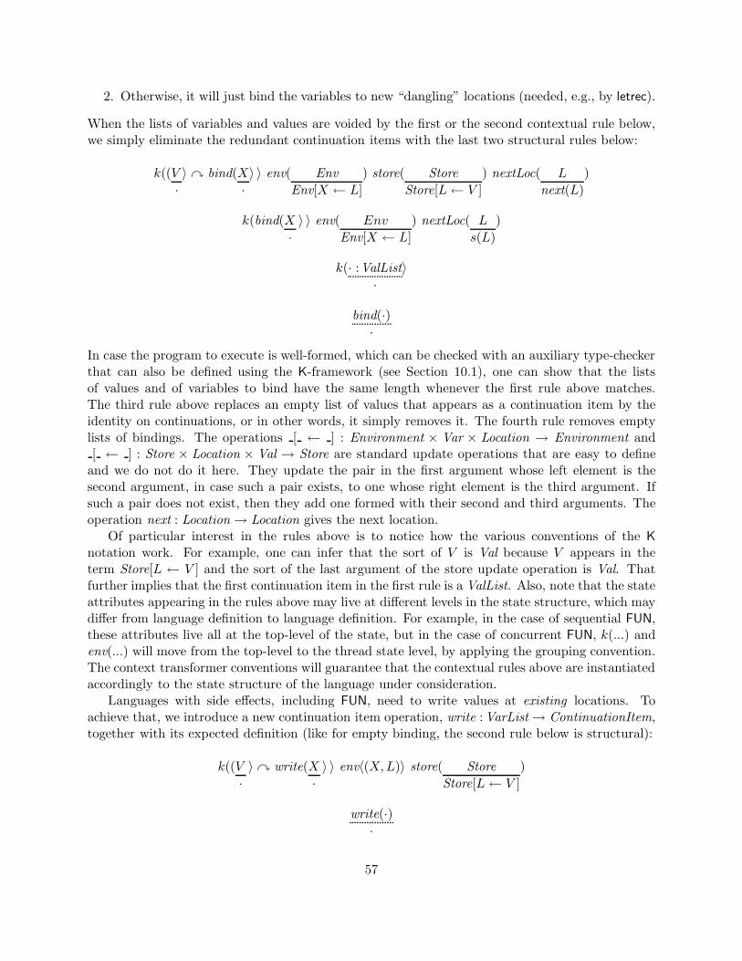
2. Otherwise, it will just bind the variables to new “dangling” locations (needed, e.g., by letrec).

When the lists of variables and values are voided by the first or the second contextual rule below,we simply eliminate the redundant continuation items with the last two structural rules below:

k((V·〉� bind(X

·〉 〉 env( Env

Env[X ← L]) store( Store

Store[L← V ]) nextLoc( L

next(L))

k(bind(X·〉 〉 env( Env

Env[X ← L]) nextLoc( L

s(L))

k(· :ValList·

〉

bind(·)·

In case the program to execute is well-formed, which can be checked with an auxiliary type-checkerthat can also be defined using the K-framework (see Section 10.1), one can show that the listsof values and of variables to bind have the same length whenever the first rule above matches.The third rule above replaces an empty list of values that appears as a continuation item by theidentity on continuations, or in other words, it simply removes it. The fourth rule removes emptylists of bindings. The operations [ ← ] : Environment × Var × Location → Environment and[ ← ] : Store × Location × Val → Store are standard update operations that are easy to define

and we do not do it here. They update the pair in the first argument whose left element is thesecond argument, in case such a pair exists, to one whose right element is the third argument. Ifsuch a pair does not exist, then they add one formed with their second and third arguments. Theoperation next : Location → Location gives the next location.

Of particular interest in the rules above is to notice how the various conventions of the Knotation work. For example, one can infer that the sort of V is Val because V appears in theterm Store[L ← V ] and the sort of the last argument of the store update operation is Val. Thatfurther implies that the first continuation item in the first rule is a ValList. Also, note that the stateattributes appearing in the rules above may live at different levels in the state structure, which maydiffer from language definition to language definition. For example, in the case of sequential FUN,these attributes live all at the top-level of the state, but in the case of concurrent FUN, k(...) andenv(...) will move from the top-level to the thread state level, by applying the grouping convention.The context transformer conventions will guarantee that the contextual rules above are instantiatedaccordingly to the state structure of the language under consideration.

Languages with side effects, including FUN, need to write values at existing locations. Toachieve that, we introduce a new continuation item operation, write :VarList→ ContinuationItem,together with its expected definition (like for empty binding, the second rule below is structural):

k((V·〉� write(X

·〉 〉 env〈(X,L)〉 store( Store

Store[L← V ])

write(·)·

57

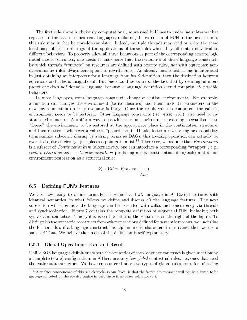
The first rule above is obviously computational, so we used full lines to underline subterms thatreplace. In the case of concurrent languages, including the extension of FUN in the next section,this rule may in fact be non-deterministic. Indeed, multiple threads may read or write the samelocations; different orderings of the applications of these rules when they all match may lead todifferent behaviors. To properly allow all these behaviors as part of the corresponding rewrite logicinitial model semantics, one needs to make sure that the semantics of those language constructsby which threads “compete” on resources are defined with rewrite rules, not with equations; non-deterministic rules always correspond to rewrite rules. As already mentioned, if one is interestedin just obtaining an interpreter for a language from its K definition, then the distinction betweenequations and rules is insignificant. But one should be aware of the fact that by defining an inter-preter one does not define a language, because a language definition should comprise all possiblebehaviors.

In most languages, some language constructs change execution environments. For example,a function call changes the environment (to its closure’s) and then binds its parameters in thenew environment in order to evaluate is body. Once the result value is computed, the caller’senvironment needs to be restored. Other language constructs (let, letrec, etc.) also need to re-store environments. A uniform way to provide such an environment restoring mechanism is to“freeze” the environment to be restored at the appropriate place in the continuation structure,and then restore it whenever a value is “passed” to it. Thanks to term rewrite engines’ capabilityto maximize sub-term sharing by storing terms as DAGs, this freezing operation can actually beexecuted quite efficiently: just places a pointer in a list.11 Therefore, we assume that Environmentis a subsort of ContinuationItem (alternatively, one can introduce a corresponding “wrapper”, e.g.,restore :Environment → ContinuationItem producing a new continuation item/task) and defineenvironment restoration as a structural rule:

k( :Val � Env·〉 env(

Env)

6.5 Defining FUN’s Features

We are now ready to define formally the sequential FUN language in K. Except features withidentical semantics, in what follows we define and discuss all the language features. The nextsubsection will show how the language can be extended with callcc and concurrency via threadsand synchronization. Figure 7 contains the complete definition of sequential FUN, including bothsyntax and semantics. The syntax is on the left and the semantics on the right of the figure. Todistinguish the syntactic constructs from other operations defined for semantic reasons, we underlinethe former; also, if a language construct has alphanumeric characters in its name, then we use asans serif font. We believe that most of the definition is self-explanatory.

6.5.1 Global Operations: Eval and Result

Unlike SOS languages definitions where the semantics of each language construct is given mentioninga complete (state) configuration, in K there are very few global contextual rules, i.e., ones that needthe entire state structure. We have encountered only two types of global rules, ones for initiating

11A trickier consequence of this, which works in our favor, is that the frozen environment will not be allowed to begarbage-collected by the rewrite engine in case there is no other reference to it.

58

the computation and the others for collecting and reporting the result of the computation. Webelieve that there is little or no chance to remove such rules entirely. Moreover, in our experience,such rules are rather meaningful and useful, because they give one a global understanding of howthe various fragments of state fit together in one’s language. We found that an early understandingof how to initiate the computation and how to retrieve the final results is so important, that weprefer to start every language definition with the semantic definitions of the global operations.

In sequential FUN we need to define an operation “eval :Exp × IntList→ IntList” which takesan expression E and an input list of integers Il and reduces to an output list of integers, theresult of evaluating E under the input Il. This operation creates an initial state containing theexpression in the continuation and the list of integers in the input buffer, all the other structuresbeing empty, nil or 0, depending on their type; this initial state is wrapped by an auxiliary operator“result :State→ IntList”, whose role is to collect the result of the computation when ready:

eval(E, Il)result(k(E) env(·) control(fstack(·) xstack(·) lstack(·)) in(Il) out(·) store(·) nextLoc(0))

The eval and result operations above divide-and-conquer the task of evaluating an expression.The contextual rules for the various language features in the sequel will all modify the state

structure wrapped by result. The result to be output is available when there is no computation tobe done in the continuation. Since the evaluation of an expression at the top of the continuationstructure wrapped by “k(...)” eventually generates a value on top of the same remaining contin-uation (empty in our case) if it terminates, we can define the semantics of result as the followingstructural rule:

result〈k( : Val) out(Il)〉Il

In words, the collected list of integers in the output buffer is returned as the result of the evalu-ation whenever there is nothing but a value in the continuation; that value left in the continuationis simply discarded, as well as all the state structures.

6.5.2 Syntactic Subcategories: Variables, Bool, Int, Real

Each syntactic subcategory of Exp needs to be given a semantics. We declared via subsorting thatvariables, booleans, integers and reals are all expressions. We split the syntactic subcategories intwo groups:

1. Syntactic subcategories that come with no meaning from their existing domain, or whoseexisting meaning is not intended to be inherited in the programming language. Variablesform such a syntactic subcategory. Variables are plain identifiers, which may come with theirsemantic definition as strings of characters, including concatenation, etc., but which is neitherinteresting nor meaningful for our purpose of using identifiers as variables. We want variablesto have the meaning of holders of values in our language, not of strings of characters. Avariable X evaluates to the value V contained in the store at the appropriate location, whichis found in the environment:

k(XV

〉 env〈(X,L)〉 store〈(L, V )〉

59

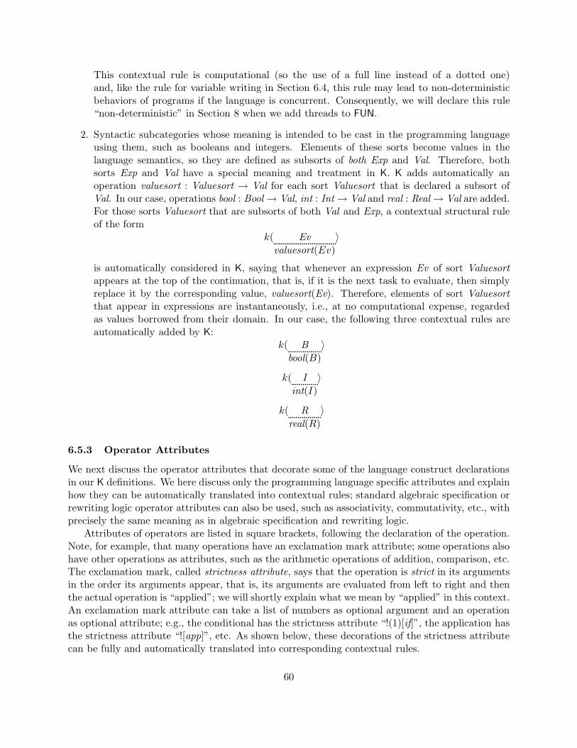
This contextual rule is computational (so the use of a full line instead of a dotted one)and, like the rule for variable writing in Section 6.4, this rule may lead to non-deterministicbehaviors of programs if the language is concurrent. Consequently, we will declare this rule“non-deterministic” in Section 8 when we add threads to FUN.

2. Syntactic subcategories whose meaning is intended to be cast in the programming languageusing them, such as booleans and integers. Elements of these sorts become values in thelanguage semantics, so they are defined as subsorts of both Exp and Val. Therefore, bothsorts Exp and Val have a special meaning and treatment in K. K adds automatically anoperation valuesort : Valuesort → Val for each sort Valuesort that is declared a subsort ofVal. In our case, operations bool : Bool→ Val, int : Int→ Val and real : Real→ Val are added.For those sorts Valuesort that are subsorts of both Val and Exp, a contextual structural ruleof the form

k( Evvaluesort(Ev)

〉

is automatically considered in K, saying that whenever an expression Ev of sort Valuesortappears at the top of the continuation, that is, if it is the next task to evaluate, then simplyreplace it by the corresponding value, valuesort(Ev). Therefore, elements of sort Valuesortthat appear in expressions are instantaneously, i.e., at no computational expense, regardedas values borrowed from their domain. In our case, the following three contextual rules areautomatically added by K:

k( Bbool(B)

〉

k( Iint(I)

〉

k( Rreal(R)

〉

6.5.3 Operator Attributes

We next discuss the operator attributes that decorate some of the language construct declarationsin our K definitions. We here discuss only the programming language specific attributes and explainhow they can be automatically translated into contextual rules; standard algebraic specification orrewriting logic operator attributes can also be used, such as associativity, commutativity, etc., withprecisely the same meaning as in algebraic specification and rewriting logic.

Attributes of operators are listed in square brackets, following the declaration of the operation.Note, for example, that many operations have an exclamation mark attribute; some operations alsohave other operations as attributes, such as the arithmetic operations of addition, comparison, etc.The exclamation mark, called strictness attribute, says that the operation is strict in its argumentsin the order its arguments appear, that is, its arguments are evaluated from left to right and thenthe actual operation is “applied”; we will shortly explain what we mean by “applied” in this context.An exclamation mark attribute can take a list of numbers as optional argument and an operationas optional attribute; e.g., the conditional has the strictness attribute “!(1)[if]”, the application hasthe strictness attribute “![app]”, etc. As shown below, these decorations of the strictness attributecan be fully and automatically translated into corresponding contextual rules.

60

If the exclamation mark attribute has a list of numbers as argument, then it means that theoperation is declared strict in those arguments in the given order. Therefore, a missing argumentof a strictness attribute is just a syntactic sugar convenience; indeed, an operator with n argumentswhich is declared just “strict” using a plain “!” attribute, is entirely equivalent to one whosestrictness attribute is “!(1 2 . . . n)”. When evaluating an operation declared using a strictnessattribute, the arguments in which the operation was declared strict (i.e., the explicit or implicitargument list of “!”) are first scheduled for evaluation; the remaining arguments need to be “frozen”until the other arguments are evaluated. If the exclamation mark attribute has an attribute, say att,then att will be used as a continuation item constructor to “wrap” the frozen arguments. Similarly,the lack of an attribute associated to a strictness attribute corresponds to a default attribute,which by convention has the same name as the corresponding operation; to avoid confusion withunderscore variables, we drop all the underscores from the original language construct name whencalculating the default name of the attribute of “!”. For example, an operation declared “ +

:Exp× Exp→ Exp [!]” is automatically desugared into “ + :Exp× Exp→ Exp [!(1 2)[+]]”.Let us next discuss how K generates corresponding rules from strictness attributes. Suppose

that we declare a strict operation, say op, whose strictness attribute’s attribute is att. Then Kautomatically adds

(a) an auxiliary operation att to the signature, whose arguments (number, order and sorts) areprecisely the arguments of op in which op is not strict; by default, the result sort of thisauxiliary operation is ContinuationItem;

(b) a rule initiating the evaluation of the strict arguments in the specified order, followed by theother arguments “frozen”, i.e., wrapped, by the corresponding auxiliary operation att.

For example, in the case of FUN’s conditional whose strictness attribute is “!(1)[if]”, an operation“if :Exp× Exp→ ContinuationItem is automatically added to the signature, together with a rule

if B then E1 else E2

B � if(E1, E2)

If the original operation is strict in all its arguments, like not, + and , then the auxiliaryoperation added has no arguments (it is a constant). For example, in the case of λK’s applicationwhose strictness attribute is “![app]”, an operation “app :→ ContinuationItem is added to thesignature, together with a rule

E El(E,El) � app

There is an additional category of attributes associated to operations that are already declaredstrict, consisting of other operations, such as +Int : Int×Int→ Int and +Real :Real×Real → Realdeclared as attributes of + :Exp × Exp → Exp. We call these attributes builtin (operation)attributes. Each of these builtin operation attributes corresponds to precisely one K-rule that“calls” the corresponding builtin operation on the right arguments. For example, the implicit rules

61

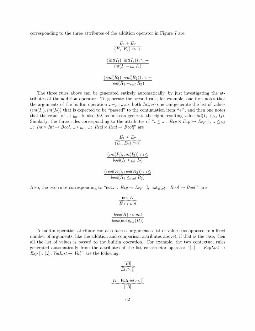
corresponding to the three attributes of the addition operator in Figure 7 are:

E1 + E2

(E1, E2) � +

(int(I1), int(I2)) � +int(I1 +Int I2)

(real(R1), real(R2)) � +real(R1 +real R2)

The three rules above can be generated entirely automatically, by just investigating the at-tributes of the addition operator. To generate the second rule, for example, one first notes thatthe arguments of the builtin operation +Int are both Int, so one can generate the list of values(int(I1), int(I2)) that is expected to be “passed” to the continuation item “+”, and then one notesthat the result of +Int is also Int, so one can generate the right resulting value int(I1 +Int I2).Similarly, the three rules corresponding to the attributes of “ ≤ : Exp × Exp → Exp [!, ≤Int

: Int× Int→ Bool, ≤Real : Real× Real→ Bool]” are

E1 ≤ E2

(E1, E2) �≤

(int(I1), int(I2)) �≤bool(I1 ≤Int I2)

(real(R1), real(R2)) �≤bool(R1 ≤real R2)

Also, the two rules corresponding to “not : Exp→ Exp [!, notBool : Bool → Bool ]” are

not E

E � not

bool(B) � notbool(notBool (B))

A builtin operation attribute can also take as argument a list of values (as opposed to a fixednumber of arguments, like the addition and comparison attributes above); if that is the case, thenall the list of values is passed to the builtin operation. For example, the two contextual rulesgenerated automatically from the attributes of the list constructor operator “[ ] : ExpList →Exp [!, [ ] :ValList→ Val]” are the following:

[El]El � []

Vl : ValList � [][Vl]

62

As the example above shows, “builtin” operation attributes need not necessarily refer only tooperations whose semantics have already been defined as part of some libraries. K simply desug-ars blindly all the operation attributes: it first adds to the signature all the operations declaredas builtin operation attributes (we here assume no errors in case of multiple declarations of thesame operator in the signature; the duplicate declarations are ignored), and then generates thecorresponding contextual rules.

There is one more case to discuss here, namely the one where the operation declared a builtinoperation attribute has no arguments, such as the operation “skip :→ Exp [unit :→ Val]”. Sinceconstant constructs are strict by default, we refrain from declaring them a strictness attribute andalso from adding the redundant continuation item. In other words, we add only one contextual rulecorresponding to the skip operation,

skip

unit

instead of the two below that one would add following blindly the general desugaring procedure (inaddition to defining the redundant operation “skip :→ ContinuationItem”):

skip

skip

skipunit

Notice that these rules associated to strictness attributes and builtin operations can applyanywhere they match, not only at the top of the continuation. In fact, the rules with exclamationmark attributes can be regarded as some sort of “precompilation rules” that transform the programinto a tree (because continuations can be embedded) that is more suitable for the other semanticrules. If, in a particular language definition, code is not generated dynamically, then these pre-compilation rules can be applied all “statically”, that is, before the semantic rules on the rightapply; one can formally prove that, in such a case, these “pre-compilation” rules need not beapplied anymore during the evaluation of the program. These rules associated to exclamationmark attributes should not be regarded as transition rules that “evolve” a program, but instead, asa means to put the program into a more convenient but computationally equivalent form; indeed,when translated into rewriting logic, the precompilation contextual rules become all equations, sothe original program and the precompiled one are in the same equivalence class, that is, they arethe same program within the initial model semantics that rewriting logic comes with.

6.5.4 The Conditional

We first translate any if then into an if then else , using the structural contextual rule

if B then E

if B then E else skip

Since the rule above is structural, it does not count as a computation step, exactly as desired.Thanks to the rule generated automatically from the strictness attribute of the conditional

constructor, we only need to define the following two (computational) rules:

63

bool(true) � if(E1, E2)E1

bool(false) � if(E1, E2)E2

Note that the expressions E1 and E2 can be pre-processed into their corresponding continuationstructures; this corresponds to “compilation-on-the-fly” and can be beneficial when executed onparallel rewrite engines12. It is interesting to note that E1 or E2 needs not be in normal form whenselected (by one of the two bottom rules above) to be placed on top of the continuation. In otherwords, some pre-processing of E1 and/or E2 may take place during the evaluation of the condition,while the remaining part of pre-processing would be performed after the expression is selected.

6.5.5 Functions

To define the semantics of functions and function applications, closure values need to be added; weintroduce a new value constructor closure :VarList × Exp × Environment → Val for this purpose.Then the semantics of function declaration is

k( fun Xl→ E

closure(Xl, E,Env)〉 env(Env)

As for the conditional, some pre-processing on-the-fly of the body of the function within the closurecan (safely) take place. Since we want to be able to exit a function abruptly using return, weneed to freeze the control state and the environment when a function is called. We do it viaa tuple operator ( , , ) that stacks useful information in fstack, as well as a continuation itempopFstack :→ ContinuationItem telling when the function call terminates; this covers the normaltermination of a function, that is, the one in which its body evaluates as a normal expression,without a return:

(k((closure(Xl, E,Env),Vl) � app � K

Vl � bind(Xl) � E � popFstack) fstack( ·

(K,Env′, C)〉 C :Ctrl) env(Env′

Env)

The control structures remain unchanged when a function returns normally, so there is no needto recover them in the rule below. However, the environment does need to change, because thefunction body is evaluated in an extended environment, namely one that provides bindings for thefunction parameters:

k( :Val � popFstackK

) fstack((K,Env, )·

〉 env(Env

)

As a general rule, if one is not sure whether certain structures in the state change or not duringthe evaluation of a particular expression or language construct, then it is safer to recover thosestructures anyway; then, if one realizes informally or proves formally that some structures do not

12There is no problem here with propagation of unexpected side effects or non-termination of rewriting, becausevalues can only be introduced at the top of the continuation attribute, k(...).

64

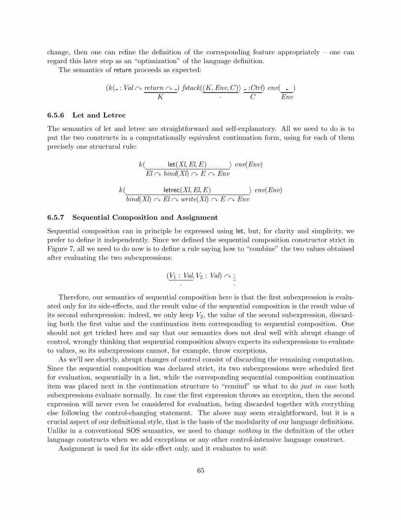
change, then one can refine the definition of the corresponding feature appropriately – one canregard this later step as an “optimization” of the language definition.

The semantics of return proceeds as expected:

(k( :Val � return �

K

) fstack((K,Env, C)·

〉 :CtrlC

) env(Env

)

6.5.6 Let and Letrec

The semantics of let and letrec are straightforward and self-explanatory. All we need to do is toput the two constructs in a computationally equivalent continuation form, using for each of themprecisely one structural rule:

k( let(Xl,El, E)El � bind(Xl) � E � Env

〉 env(Env)

k( letrec(Xl,El, E)bind(Xl) � El � write(Xl) � E � Env

〉 env(Env)

6.5.7 Sequential Composition and Assignment

Sequential composition can in principle be expressed using let, but, for clarity and simplicity, weprefer to define it independently. Since we defined the sequential composition constructor strict inFigure 7, all we need to do now is to define a rule saying how to “combine” the two values obtainedafter evaluating the two subexpressions:

(V1 : Val·

, V2 : Val) � ;·

Therefore, our semantics of sequential composition here is that the first subexpression is evalu-ated only for its side-effects, and the result value of the sequential composition is the result value ofits second subexpression: indeed, we only keep V2, the value of the second subexpression, discard-ing both the first value and the continuation item corresponding to sequential composition. Oneshould not get tricked here and say that our semantics does not deal well with abrupt change ofcontrol, wrongly thinking that sequential composition always expects its subexpressions to evaluateto values, so its subexpressions cannot, for example, throw exceptions.

As we’ll see shortly, abrupt changes of control consist of discarding the remaining computation.Since the sequential composition was declared strict, its two subexpressions were scheduled firstfor evaluation, sequentially in a list, while the corresponding sequential composition continuationitem was placed next in the continuation structure to “remind” us what to do just in case bothsubexpressions evaluate normally. In case the first expression throws an exception, then the secondexpression will never even be considered for evaluation, being discarded together with everythingelse following the control-changing statement. The above may seem straightforward, but it is acrucial aspect of our definitional style, that is the basis of the modularity of our language definitions.Unlike in a conventional SOS semantics, we need to change nothing in the definition of the otherlanguage constructs when we add exceptions or any other control-intensive language construct.

Assignment is used for its side effect only, and it evaluates to unit:

65

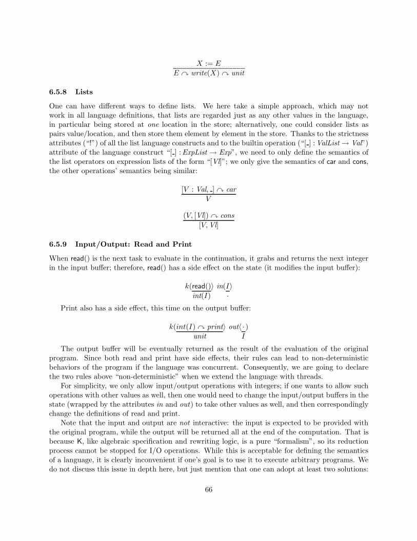
X := E

E � write(X) � unit

6.5.8 Lists

One can have different ways to define lists. We here take a simple approach, which may notwork in all language definitions, that lists are regarded just as any other values in the language,in particular being stored at one location in the store; alternatively, one could consider lists aspairs value/location, and then store them element by element in the store. Thanks to the strictnessattributes (“!”) of all the list language constructs and to the builtin operation (“[ ] :ValList→ Val”)attribute of the language construct “[ ] :ExpList → Exp”, we need to only define the semantics ofthe list operators on expression lists of the form “[Vl]”; we only give the semantics of car and cons,the other operations’ semantics being similar:

[V : Val, ] � carV

(V, [Vl]) � cons[V,Vl]

6.5.9 Input/Output: Read and Print

When read() is the next task to evaluate in the continuation, it grabs and returns the next integerin the input buffer; therefore, read() has a side effect on the state (it modifies the input buffer):

k(read()int(I)

〉 in(I·〉

Print also has a side effect, this time on the output buffer:

k(int(I) � printunit

〉 out〈 ·I

)

The output buffer will be eventually returned as the result of the evaluation of the originalprogram. Since both read and print have side effects, their rules can lead to non-deterministicbehaviors of the program if the language was concurrent. Consequently, we are going to declarethe two rules above “non-deterministic” when we extend the language with threads.

For simplicity, we only allow input/output operations with integers; if one wants to allow suchoperations with other values as well, then one would need to change the input/output buffers in thestate (wrapped by the attributes in and out) to take other values as well, and then correspondinglychange the definitions of read and print.

Note that the input and output are not interactive: the input is expected to be provided withthe original program, while the output will be returned all at the end of the computation. That isbecause K, like algebraic specification and rewriting logic, is a pure “formalism”, so its reductionprocess cannot be stopped for I/O operations. While this is acceptable for defining the semanticsof a language, it is clearly inconvenient if one’s goal is to use it to execute arbitrary programs. Wedo not discuss this issue in depth here, but just mention that one can adopt at least two solutions:

66

1. slightly modify the semantics to use a rewrite engine feature such as Maude’s loop mode [5]which was designed specifically for dealing with I/O and user interaction; or

2. provide functionality in the rewrite engine to link certain lists to I/O buffers.

6.5.10 Parametric Exceptions

Parametric exceptions can be defined with just three contextual rules (we do not count the trivialone generated automatically from the strictness attribute of throw):

1. One structural rule for initiating the evaluation of the try catch( ) statement. Operation“popXstack :→ ContinuationItem” is needed to mark the execution of the main body of theexception code; returning information is also stacked with a tupling operation:

(k(try E′ catch(X) E � K

E′ � popXstack) xstack( ·

(X,E,Env,K,C)〉 C :Ctrl) env(Env)

2. One structural contextual rule for normal, non-exceptional evaluation. If E′ evaluates nor-mally, i.e., if its evaluation does not encounter any exception throwing, then the execution isrecovered with the original continuation; note that one only needs to recover the continuation,the other control ingredients being the same:

k( :Val � popXstackK

) xstack(( , , ,K, )·

〉

3. One for performing the actual change of context in case of an exception throwing. Theexpression which is thrown is first evaluated (note that there is no problem if that expressionthrows itself an exception) and then its value is bound to the parameter and the executioncontext recovered:

(k( :Val � throw �

bind(X) � E � Env � K

) xstack((X,E,Env,K,C)·

〉 :CtrlC

) env(Env

)

6.5.11 Loops with Break and Continue

Because of break and continue, which have a similar behavior to (non-parametric) exceptions, anadditional stack for loops is necessary in the control soup of the state. Also, a helping specialcontinuation marker “ � :→ ContinuationItem” is defined. Since continue has a more generalsemantics for “for” loops than for “while” loops (the “step”, J below, is executed), we first translate“while” into “for” using a structural rule:

while(B) Efor(skip; B; skip) E

Whenever a loop is encountered, an appropriate execution context is created, by stacking informa-tion needed to recover in case of a “break” or “continue”:

67

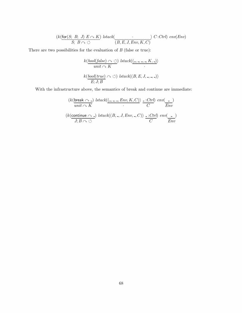
(k(for(S; B; J) E � K

S; B � �) lstack( ·

(B,E, J,Env,K,C)〉 C :Ctrl) env(Env)

There are two possibilities for the evaluation of B (false or true):

k(bool(false) � �unit � K

) lstack(( , , , ,K, )·

〉

k(bool(true)E; J;B

� �) lstack((B,E, J, , , )〉

With the infrastructure above, the semantics of break and continue are immediate:

(k(break �

unit � K

) lstack(( , , ,Env,K,C)·

〉 :CtrlC

) env(Env

)

(k(continue �

J;B � �) lstack((B, , J,Env, , C)〉 :Ctrl

C

) env(Env

)

68

7 Defining KOOL: An Object-Oriented Language

NEXT-VERSION:

69

8 On Modular Language Design

We here show how the K framework addresses the important aspect of modularity in programminglanguage definition and design. By “modular” in this context it is meant significantly more thanjust grouping together all the rules corresponding to a particular language feature in a module,which is ultimately what most existing language definitional frameworks do anyway, formally orinformally. What a framework supporting modular language design means here is one having

the capability to add or remove programming language features without a need to modifyany of the other, unrelated language features.

Most existing definitional frameworks either cannot support properly some important languagefeatures at all, or when they do, they do not do it in a modular manner. A notorious example isthe big-step SOS, also called “natural” semantics and discussed in Section 4.1, which cannot beused at all to define non-trivial concurrent programming languages, and which is hardly suitablefor defining features that change the control abruptly, such as exceptions, halt, break, continue, etc.For example, to define an innocent “halt(E)” statement, one would need to add for each existinglanguage construct as many new rules as subexpressions that can halt the program that languageconstruct has. From a modular language design perspective, it is hard to imagine anything worsethan that in a language definitional framework.

In this section we discuss the modularity of K both empirically and theoretically. Empirically,we first show how several variations of a simple language can be accomodated in K with minimalchanges, and then show how one can add to the sequential FUN language defined in the previoussection two important and nontrivial features, namely a callcc construct and concurrency via threadsand synchronization with locks. Figure 9 shows the new operations and rules that need to be addedand the changes that need to be applied to the definition of sequential FUN to accommodate thenew language features; note that no change needs to be done to support callcc, and that thechanges needed to support concurrency are global, not specific to other language features. Onthe theoretical side, we show how Modular SOS (MSOS) [21], designed specifically to address thelack of modularity of standard SOS, can be translated into K. This is not surprising, because Kis rewriting logic and MSOS has already been shown to map into rewriting logic [4], but it isinstructive because it shows the connections and relationships between two modular frameworks.

8.1 Variations of a Simple Language

The simplest and most effective way to show the modularity capabilities of a language definitionalframework is by means of a convincing example. Such an example was presented in [29], to show thestrengths of monads in defining interpreters in the context of a pure functional language, namelyHaskell. Monads [20, 15] increase the ease with which (functional) programs may be non-triviallymodified, and can mimic the effects of impure features, such as different types of exceptions andstates. The overall point of [29] is that one could use monads to capture modularly the differentdesired variations of an interpreter, including the addition of impure features. In order to definesuch a variation, all one needs to do is to redefine the corresponding monad and to locally modifythe existing definitions of some, typically very few, of the other language statements, namely ofthose that “interact” with the new feature.

In what follows we show how one can define, using K, the different variations of the simpleλ-calculus with integers language from [29]. We start with the K-definition of λ-calculus with

70

Variation Zero: Standard Interpreter (outputting string messages instead of values)import STRING

showval : Val→ String}

. . . . . . . . . . . . . . . . . . . . . . . . . . . . . . . . . . . . . . .{

showval(int(I)) = showint(I)showval(closure( , , )) = "function"

eval :Exp→ Stringresult :State→ String

}. . . . . . . . . . . . . . . . . . . . . . . . . . . . . . . . . . . . . . . . . . . . . . .

{result〈k(V :Val)〉 = showval(V )

Variation One: Error Messages

error : String→ ContinuationItem}

. . . .

⎧⎪⎪⎪⎪⎪⎪⎪⎪⎪⎪⎨⎪⎪⎪⎪⎪⎪⎪⎪⎪⎪⎩

result〈k(V :Val)〉 = "Success: " ++ showval(V )result〈k(error(str)〉〉 = "Error: " ++ strk( X :Var

error("unbound variable: " ++ X)〉

k( (V1, V2) � +error("should be numbers:"++showval(V1)++showval(V2))

〉

k( (V, ) � apperror("should be function: " ++ showval(V ))

〉

Variation Two: Error Messages with Positions

pos : Position → StateAttribute [struct]reset : Position→ ContinuationItemAt : Position × Exp→ Exp

⎫⎬⎭ . . . .

⎧⎪⎪⎪⎪⎪⎪⎨⎪⎪⎪⎪⎪⎪⎩

eval(E) = result(k(E) env(·) store(·) nextLoc(0) pos(0))k( At(P, E)

E � reset(P ′)〉 pos(P ′

P)

k(reset(P )·〉 pos(

P)

result〈k(error(str)〉 pos(P )〉 = showpos(P )++":Error:"++str

Variation Three: State

tick : Int→ StateAttribute [struct]Count : → Exp

}. . . . . .

⎧⎪⎪⎪⎪⎪⎪⎪⎪⎨⎪⎪⎪⎪⎪⎪⎪⎪⎩

eval(E) = result(k(E) env(·) store(·) nextLoc(0) tick(0))k((closure(X, E,Env), V ) � app

V � bind(X) � E � Env′� K) env(Env′

Env) tick( I

I + 1)

k((int(I1), int(I2)) � +int(I1 +Int I2)

〉 tick( II + 1

)

k(Count �

int(I)) tick(I)

Variation Four: Output

out :String→StateAttribute [struct]Out : Exp→ Exp [!]

}. . .

⎧⎪⎪⎨⎪⎪⎩

eval(E) = result(k(E) env(·) store(·) nextLoc(0) out(""))k(V � Out

·〉 out( O

O ++ showval(V ) ++ ";")

result〈k(V :Val) out(O)〉="Output:"++showval(V )++"Value:"++O

Variation Five: Nondeterministic Choice

Fail :→ ExpAmb : Exp× Exp→ Exp

}. . . . . . . . . . . . . . . . . . . . . . . . . . . . . . . . . . . . . . . . . . . . . . . . . . . . . . . . . . . .

⎧⎪⎪⎪⎪⎪⎪⎪⎪⎪⎪⎨⎪⎪⎪⎪⎪⎪⎪⎪⎪⎪⎩

result〈k(Fail〉〉""

k(Amb(E1, E2)E1

〉

k(Amb(E1, E2)E2

〉

Variation Five’: Nondeterministic Choice (simulated, a la [29])

eval :Exp→ StringListFail :→ ExpAmb : Exp× Exp→ Exp

⎫⎬⎭ . . . . . . . . . . . . . . . . . . . . . . . . . . . . . . . . .

⎧⎪⎪⎨⎪⎪⎩

result〈k(Fail〉〉·result(k(Amb(E1, E2) � K) R)

result(k(E1 � K) R), result(k(E2 � K) R)

Figure 8: Variations of the λ-calculus language in Figure 1.

71

integers language in Figure 1, which is essentially the same base language as the one in [29]; theonly difference is that we consider addition to be an infix operation (“ + ”) instead of a prefix one(“Add ”). Note also that our definition in Figure 1 is purely equational, while the one in [29] usessome of the strengths of the underlying Haskell language, such as bindings, higher-order functionsand their application, as well as the controled, lazy evaluation mechanism. Despite the fact thatour language definitions are all based on a generic notion of state, they are still pure, in the sensethat they are nothing but equational theories when the language is deterministic, or more generalrewrite logic theories when the language to define is non-deterministic or concurrent. Our notionof state is very generous, in the sense that it can contain anything, including the program itself; inparticular, it is not constrained to contain a store or an environment, even though many definitionsof (pure or impure) languages prefer these.

a deeper comparison here, or in the intro, between unrestricted equational logic and itsrestricted use in Haskell-like languages?

There are six variations of this language discussed in [29], each extending the standard inter-preter with a new feature, such as (1) error messages, (2) error messages with positions, (3) stateand statement counting , (4) output, (5) non-deterministic choice, and (6) propogating state back-wards. While (6) is an interesting programming technique in the context of lazy languages, we findno use for it in the context of defining programming languages, so we do not discuss it here. Atthe end of each section defining a variation of the interpreter in [29], a short discussion is given onhow difficult it would be for an “impure language” to modify the existing interpreter to accountfor the new feature. We agree with those comments, but want to reemphasize that our algebraicframework is also pure, even though it is inherently state-based: term rewriting is all about match-ing and iteratively transforming a term; if “term” is read “state”, as we frequently prefer to do inthis paper, then our framework may wrongly appear to be “impure” to a hasty reader.

The equational and rewriting logic based K language definitional framework that we use in thispaper is algebraic, logical and model-theoretically meaningful, so it is as pure as a language canbe. Indeed, we show that the language variations in [29] can be very elegantly accomodated in K,at some extent even more elegantly than using the monadic approach. More importantly, as shownshortly, we can combine the language features introduced by these variations without having tochange any of their local definitions! The only changes that are required are global: the structureof the state, the initial state, and the result reporting operations.

The modifications that are needed to the K definition in Figure 1 to accomodate all the otherfive variations are shown in Figure 8 and discussed next. We argue that the changes required inK to accommodate each variation are minimal and unavoidable; in particular, K requires fewerchanges than the monadic approach. Our claims apply, of course, to this simple experiment; we donot know how to formalize in general that a language definitional framework requires a “minimal”number of changes in a language definition when adding a new feature.

Variation Zero: Standard Interpreter

In a standard interpreter one would like to report the results of computations or error messages ina readable format to the user. Our equational theory definition in Figure 1 is purely mathematical,with no consideration for readability of results when used as the input of a rewrite engine, thusbecomming an interpreter. Like in [29], we next report results and messages as strings; we therefore

72

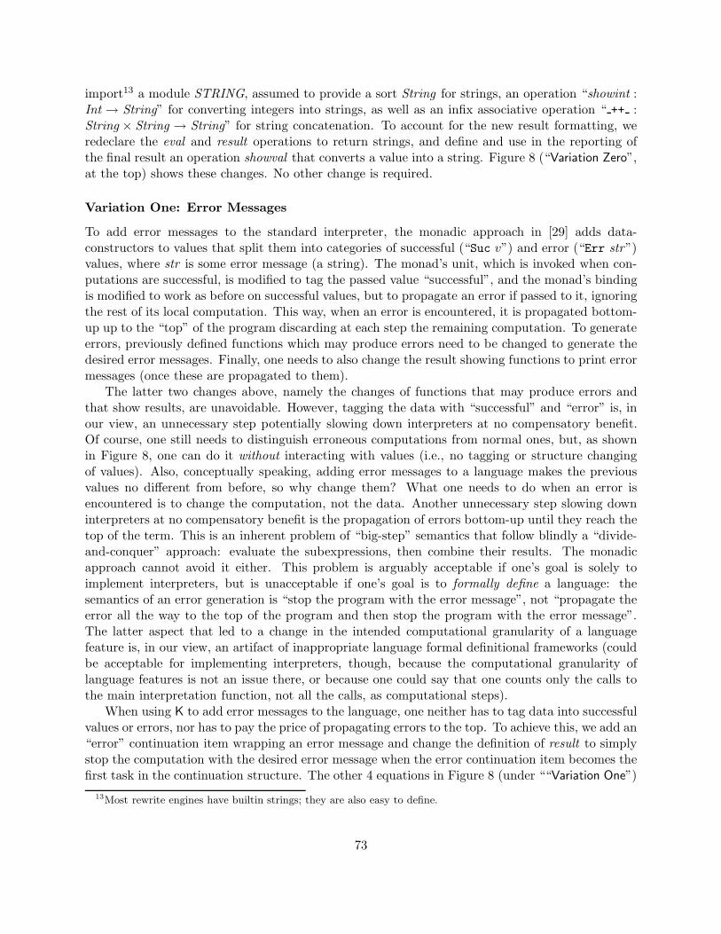
import13 a module STRING, assumed to provide a sort String for strings, an operation “showint :Int → String” for converting integers into strings, as well as an infix associative operation “ ++ :String × String → String” for string concatenation. To account for the new result formatting, weredeclare the eval and result operations to return strings, and define and use in the reporting ofthe final result an operation showval that converts a value into a string. Figure 8 (“Variation Zero”,at the top) shows these changes. No other change is required.

Variation One: Error Messages

To add error messages to the standard interpreter, the monadic approach in [29] adds data-constructors to values that split them into categories of successful (“Suc v”) and error (“Err str”)values, where str is some error message (a string). The monad’s unit, which is invoked when con-putations are successful, is modified to tag the passed value “successful”, and the monad’s bindingis modified to work as before on successful values, but to propagate an error if passed to it, ignoringthe rest of its local computation. This way, when an error is encountered, it is propagated bottom-up up to the “top” of the program discarding at each step the remaining computation. To generateerrors, previously defined functions which may produce errors need to be changed to generate thedesired error messages. Finally, one needs to also change the result showing functions to print errormessages (once these are propagated to them).

The latter two changes above, namely the changes of functions that may produce errors andthat show results, are unavoidable. However, tagging the data with “successful” and “error” is, inour view, an unnecessary step potentially slowing down interpreters at no compensatory benefit.Of course, one still needs to distinguish erroneous computations from normal ones, but, as shownin Figure 8, one can do it without interacting with values (i.e., no tagging or structure changingof values). Also, conceptually speaking, adding error messages to a language makes the previousvalues no different from before, so why change them? What one needs to do when an error isencountered is to change the computation, not the data. Another unnecessary step slowing downinterpreters at no compensatory benefit is the propagation of errors bottom-up until they reach thetop of the term. This is an inherent problem of “big-step” semantics that follow blindly a “divide-and-conquer” approach: evaluate the subexpressions, then combine their results. The monadicapproach cannot avoid it either. This problem is arguably acceptable if one’s goal is solely toimplement interpreters, but is unacceptable if one’s goal is to formally define a language: thesemantics of an error generation is “stop the program with the error message”, not “propagate theerror all the way to the top of the program and then stop the program with the error message”.The latter aspect that led to a change in the intended computational granularity of a languagefeature is, in our view, an artifact of inappropriate language formal definitional frameworks (couldbe acceptable for implementing interpreters, though, because the computational granularity oflanguage features is not an issue there, or because one could say that one counts only the calls tothe main interpretation function, not all the calls, as computational steps).

When using K to add error messages to the language, one neither has to tag data into successfulvalues or errors, nor has to pay the price of propagating errors to the top. To achieve this, we add an“error” continuation item wrapping an error message and change the definition of result to simplystop the computation with the desired error message when the error continuation item becomes thefirst task in the continuation structure. The other 4 equations in Figure 8 (under ““Variation One”)

13Most rewrite engines have builtin strings; they are also easy to define.

73

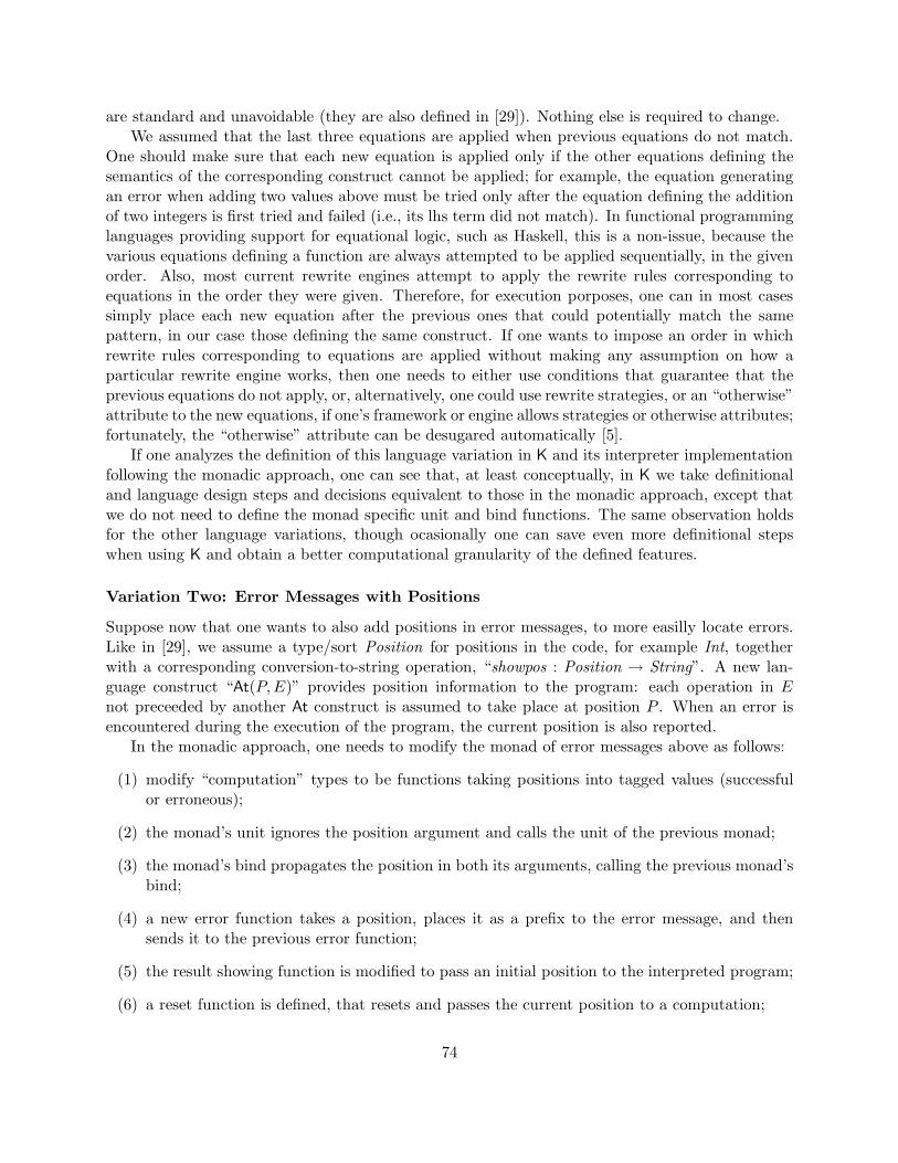
are standard and unavoidable (they are also defined in [29]). Nothing else is required to change.We assumed that the last three equations are applied when previous equations do not match.

One should make sure that each new equation is applied only if the other equations defining thesemantics of the corresponding construct cannot be applied; for example, the equation generatingan error when adding two values above must be tried only after the equation defining the additionof two integers is first tried and failed (i.e., its lhs term did not match). In functional programminglanguages providing support for equational logic, such as Haskell, this is a non-issue, because thevarious equations defining a function are always attempted to be applied sequentially, in the givenorder. Also, most current rewrite engines attempt to apply the rewrite rules corresponding toequations in the order they were given. Therefore, for execution porposes, one can in most casessimply place each new equation after the previous ones that could potentially match the samepattern, in our case those defining the same construct. If one wants to impose an order in whichrewrite rules corresponding to equations are applied without making any assumption on how aparticular rewrite engine works, then one needs to either use conditions that guarantee that theprevious equations do not apply, or, alternatively, one could use rewrite strategies, or an “otherwise”attribute to the new equations, if one’s framework or engine allows strategies or otherwise attributes;fortunately, the “otherwise” attribute can be desugared automatically [5].

If one analyzes the definition of this language variation in K and its interpreter implementationfollowing the monadic approach, one can see that, at least conceptually, in K we take definitionaland language design steps and decisions equivalent to those in the monadic approach, except thatwe do not need to define the monad specific unit and bind functions. The same observation holdsfor the other language variations, though ocasionally one can save even more definitional stepswhen using K and obtain a better computational granularity of the defined features.

Variation Two: Error Messages with Positions

Suppose now that one wants to also add positions in error messages, to more easilly locate errors.Like in [29], we assume a type/sort Position for positions in the code, for example Int, togetherwith a corresponding conversion-to-string operation, “showpos : Position → String”. A new lan-guage construct “At(P,E)” provides position information to the program: each operation in Enot preceeded by another At construct is assumed to take place at position P . When an error isencountered during the execution of the program, the current position is also reported.

In the monadic approach, one needs to modify the monad of error messages above as follows:

(1) modify “computation” types to be functions taking positions into tagged values (successfulor erroneous);

(2) the monad’s unit ignores the position argument and calls the unit of the previous monad;

(3) the monad’s bind propagates the position in both its arguments, calling the previous monad’sbind;

(4) a new error function takes a position, places it as a prefix to the error message, and thensends it to the previous error function;

(5) the result showing function is modified to pass an initial position to the interpreted program;

(6) a reset function is defined, that resets and passes the current position to a computation;

74

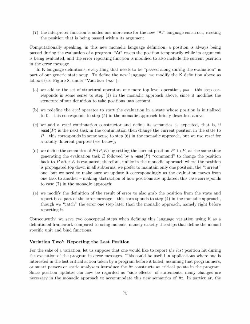
(7) the interpreter function is added one more case for the new “At” language construct, resetingthe position that is being passed within its argument.

Computationally speaking, in this new monadic language definition, a position is always beingpassed during the evaluation of a program, “At” resets the position temporarily while its argumentis being evaluated, and the error reporting function is modified to also include the current positionin the error message.

In K language definitions, everything that needs to be “passed along during the evaluation” ispart of our generic state soup. To define the new language, we modify the K definition above asfollows (see Figure 8, under “Variation Two”):

(a) we add to the set of structural operators one more top level operation, pos – this step cor-responds in some sense to step (1) in the monadic approach above, since it modifies thestructure of our definition to take positions into account;

(b) we redefine the eval operator to start the evaluation in a state whose position is initializedto 0 – this corresponds to step (5) in the monadic approach briefly described above;

(c) we add a reset continuation constructor and define its semantics as expected, that is, ifreset(P ) is the next task in the continuation then change the current position in the state toP – this corresponds in some sense to step (6) in the monadic approach, but we use reset fora totally different purpose (see below);

(d) we define the semantics of At(P,E) by setting the current position P ′ to P , at the same timegenerating the evaluation task E followed by a reset(P ) “command” to change the positionback to P after E is evaluated; therefore, unlike in the monadic approach where the positionis propagated top down in all subterms, we prefer to maintain only one position, the “current”one, but we need to make sure we update it correspondingly as the evaluation moves fromone task to another – making abstraction of how positions are updated, this case correspondsto case (7) in the monadic approach;

(e) we modify the definition of the result of error to also grab the position from the state andreport it as part of the error message – this corresponds to step (4) in the monadic approach,though we “catch” the error one step later than the monadic approach, namely right beforereporting it.

Consequently, we save two conceptual steps when defining this language variation using K as adefinitional framework compared to using monads, namely exactly the steps that define the monadspecific unit and bind functions.

Variation Two’: Reporting the Last Position

For the sake of a variation, let us suppose that one would like to report the last position hit duringthe execution of the program in error messages. This could be useful in applications where one isinterested in the last critical action taken by a program before it failed, assuming that programmers,or smart parsers or static analyzers introduce the At constructs at critical points in the program.Since position updates can now be regarded as “side effects” of statements, many changes arenecessary in the monadic approach to accommodate this new semantics of At. In particular, the

75

computation type of the monad needs to be a function from positions to pairs containing a taggedvalue and another position. Almost all the definitions in the previous monad need to change,because, from a monadic perspective, this change in the semantics of At is a radical one: theinterpreter needs to have a state now, like in the next variation.

It is straighforward to change our K definition to accomodate this simple variation of thelanguage. We only need to drop the reset continuation item constructor and its corresponding rule,and to change the semantics of At to the following simpler one:

k(At(P,E)E

〉 pos(P

)

Variation Three: State

Many programming languages are crucially based on some notion of state. To add state to an inter-preter implemented using the monadic approach, one needs to define a monad whose computationtypes are functions taking states into pairs consisting of a value and a state, to define the monad’sunit to keep the state unchanged, and to define the monad’s bind to collect the updated state fromits first argument and then pass it to its second argument. The idea of the state monad is thereforeto propagate the state changes sequentially. To exemplify the use of the state monad, [29] proposesa simple variation of the language which counts the number of addition or application operationsduring the execution of the program, and enriches the language with a Count construct which stopsthe program and returns the value of the counter as a result. Besides having to define the statemonad (instantiated for the simple state required by this language), in the monadic approach onealso needs to add a “tick” function for incrementing the counter, and then to change the definitionsof addition and application to invoke this function. Finally, to retrieve the value of the counterneeded for the semantics of Count, a “fetch” function needs to be defined that extracts the counterfrom the state.

Let us now discuss the K definition in Figure 8. We add one more state attribute, tick, whichkeeps the counter. The evaluation of the program (the definition of eval) starts with counter 0.The rules defining application and addition are modified to increment the counter (nothing elsechanges in those rules except the increment of the counter). Finally, the semantics of Count isdefined straightforwardly: fetch the counter (without a need to define a special “fetch” operator orfunction) and replace the entire computation by its corresponding value. Nothing else changes.

Variation Four: Output

To generate output, a language construct Out(E) can be added, which evaluates E normally tosome value V , then it outputs V , and then returns V as the result of its own evaluation. Toadd output using the monadic approach, [29] defines a new monad whose computation type is apair containing a string (the collected output) and a value, whose unit generates an empty stringkeeping the value, and whose bind collects the outputs of its two arguments and concatenates them,propagating the values as before. A result showing function is also needed to print both the finaloutput and the value of the program. A new clause in the interpreter is also required, interpretingOut(E) as expected: interpret E then output its value.

Figure 8 shows the changes needed in K to add output. We start by adding a state attributeout for collecting the output; if the underlying rewrite engine permits it (e.g., Maude [] does; note,

76

however, that this action unavoidably affects the purity of the definitional framework), one canlink this attribute to a standard output or socket to output the results incrementally, as they aregenerated. The initial state contains the empty string as an output. We then define the languageconstruct out to be strict (the “!” attribute); recall that a continuation item Out is also added.The semantics of Out is as expected: when passed a value at the top of the continuation, Outdisolves itself and the value is appended to the output. Finally, we modify the result to print thesame output as in [29].

Variations Five and Five’: Nondeterministic Choice

Nondeterminism and concurrency are delicate subjects in the functional programming commu-nity. Their blind integration destroys the functional behavior of programs. In particular, it isimpossible to extend an interpreter function with a clause for a non-deterministic choice languageconstruct, simply because the interpreter function would not be a function anymore. To determinizea non-deterministic language in a functional environment, one would need to either implement adeterministic scheduler or collect all possible results that a program can evaluate to into a listor a set. We find both these approaches unsatisfactory from a language design perspective: thefirst because a particular scheduling is imposed, so the language only appears to be but it is notdeterministic anymore, and the second because one does not get an interpreter for the language.Indeed, the monadic approach in [29] opts for the latter and calls the resulting interpreter one that“deals with” a non-deterministic language. Before we discuss the approach in [29] and show howwe can obtain the same result, we prefer to first show how easily a non-deterministic choice featurecan be defined in a framework that provides natural support for non-determinism and concurrency,and, consequently, how one can obtain an interpreter for a nondeterministic language.

We consider the same illustrory language constructs Fail and Amb(E1, E2) as [29], the first forfailing an execution with no output and the second for ambiguously choosing E1 or E2. Figure 8(under “Variation Five”) shows that no change is required to the existing code, but three new rulesneed to be added: one for Fail and two for Amb. Note that the rules for Amb are boxed, meaningthat they are nondeterministic, so they are assumed to be rewrite rules in the corresponding rewritelogic theory. We could have also defined Amb to be commutative and then added only one boxedrule, say the first. If one is interested in obtaining an interpreter then all what needs to do is torun this theory on a rewrite engine. On more advanced engines, such as Maude, one can evenenable different rewrite strategies, including ones based on fairness, potentialy obtaining any ofthe possible behaviors of the program. If the language designer wants to explicitly see whethera particular result can be obtained, or all the results that can be obtained, then one can use areachability analysis tool; for example, Maude has a command “search” exactly for this purpose.Morover, if the statespace is finite then one can also see and even model-check (e.g., using the LTLmodel-checking command “model-ckeck of Maude) the entire graph associated to the execution ofa non-deterministic program.

Even though a “search eval(p) =>* S:String” command in a language like Maude wouldlist all the values that program p can evaluate to and thus obtain the same effect as the monadicextension in [29] (based on defining a monad of lists, whose binding is list comprehension), we alsoshow in Figure 8 (under “Variation Five’”) how one can explicitly obtain an interpreter that “dealswith” a nondeterministic language, that is, one that deterministically collects all possible valuesthat the program can evaluate to. We first need to modify the eval operation to return a list ofresults. To be faithful to [29] we modify the result of Fail to return the empty list. The tricky part

77

The definition of sequential FUN inFigure 7 needs to change as follows:1) add callcc and its two rules below2) replace structural operators with

the ones in the picture to the right3) replace eval and result definitions as below4) declare non-deterministic the rulesfor write, variable lookup, read and print5) add six more rules for threads:

a) one rule for creation of threadsand one for termination of threads;

b) two rules for acquiring a lockc) two rules for releasing a lock

No other changes needed.

Structural operations

CtrlContinuation

FunctionStack ExceptionStack LoopStack

k

fstack xstack lstack

Environment= VarLocSet

IntListIntList Nat

env control

LocValSet

State

outin storenextLoc

ThreadState

IntIntSet

holds

IntSet

busythread *

newThread :Exp × Environment → StateAttribute¯

. . . .

8>>>>>>>>>><>>>>>>>>>>:

eval(E, Il)result(newThread(E, ·) busy(·) in(Il) out(·) store(·) nextLoc(0))

result(busy( ) in( ) out(Il) store( ) nextLoc( ))Il

newThread(E, Env)thread(k(E) env(Env) control(fstack(·) xstack(·) lstack(·)) holds(·))

callcc : Exp→ Exp [!]cc :Continuation ×Ctrl× Environment→ Val

ff. . . . . . . . . . . . . . . . . . . .

8>><>>:

(k( V :Val � callcc(V, cc(K, C,Env)) � app

� K) C :Ctrl) env(Env)

(k(((cc(K, C,Env), V ) � app �

V � K) :Ctrl

C) env(

Env)

spawn : Exp→ Expacquire : Exp→ Exp [!]release : Exp→ Exp [!]

9=; . . . . . . . . . . .

8>>>>>>>>>>><>>>>>>>>>>>:

thread〈k(spawn(E)

unit〉 env(Env)〉 ·

newThread(E, Env)thread〈k( :Val) holds(LCs)〉

·busy( Is

Is − LCs) k(int(I) � acquire

unit〉 holds〈(I, N

s(N))〉

k(int(I) � acquireunit

〉 holds〈 ·(I, 0)

〉 busy( IsIs, I

)⇐ not(I in Is)

k(int(I) � releaseunit

〉 holds〈(I, s(N)N

)〉 k(int(I) � releaseunit

〉 holds〈(I, 0)·〉 busy〈I

·〉

Figure 9: Adding call/cc and threads to FUN

is the definition of Amb(E1, E2): we match the entire result(...) term whose next computationaltask is an ambiguous construct followed by continuation K and whose rest of state ingredients (i.e.,store, environment, etc.) are R, and rewrite it in two similar terms separated by the list constructorfor StringList, one for E1 and the other for E2. This way, we obtain as final result a list of 2n

strings, where n is the number of Amb constructs appearing in the language. If one wants to obtaina set of results instead of a list, all one needs to do is to replace the sort StringList by StringSetand remove the one-character comma list constructor between the two generated result terms (theset constructor is the concatenation operator “ ”).

8.2 Adding Call/cc to FUN

Call with the current continuation, or call/cc, is a very powerful control-intensive language con-struct. Scheme is one of the most known languages providing an explicit call/cc construct, thoughother languages also provide it, or at least some limited version of it. Briefly, call/cc takes an

78

argument, expected to evaluate to a function, and passes it the current computation context. Ifthe function that was the argument of call/cc passes its argument any value, then the computationis reset back to the point the call/cc took place. This can be regarded as a jump back in time,recovering also the original computation context. Because of the variety of control-intensive FUNlanguage constructs, call/cc in FUN needs to freeze more than the current continuation. It mustactually freeze the entire control context. To understand why this is needed, imagine that thecall/cc appears in the body of some function, in some nested loops and try/catch blocks; once avalue is passed back to the context in which the call/cc took place, one would, obviously, wantto still be able to returning from the function using return, to breaking/continuing loops, as wellas to throwing exceptions, exactly like in the original context. Therefore, in our language, call/ccappears to better abbreviate “call with current context”.

Even though call/cc is conceptually more powerful than our other control-intensive languageconstructs (their translation would be technically involved, though), it is actually very easy todefine in our framework. A special “current context” value is needed, so we define an operationcc :Continuation × Ctrl × Environment → Val, as well as a corresponding continuation item,callcc :→ ContinuationItem. Note that callcc is declared strict in its argument. When a value(expected to be a function closure, namely the evaluated argument expression of callcc) is passedto it at the top of the continuation, a special “control context” value is created and passed to itsargument function:

(k( V :Val � callcc(V, cc(K,C,Env)) � app

� K) C :Ctrl) env(Env)

If the special control context value is ever passed a value, then the original execution context isrestored and the value is passed to it:

(k(((cc(K,C,Env), V ) � app �

V � K

) :CtrlC

) env(Env

)

8.3 Adding Concurrency to FUN

To add threads to a language, the structure of the state typically needs to change. That is becausethreads contain and repeat part of the state, including a continuation, an environment and a controlstructure. The picture in Figure 9 shows the new structure of the state of FUN. There are severalnew attributes and some old ones have been restructured:

• An attribute thread has been added, which is allowed to multiply as part of the state (becauseof the star “�” on its edge to State);

• The continuation, environment and control previously at the top level in the state, weremoved within the thread attribute; indeed, each thread needs enough functionality to carryover its own computation; the store will be shared among all threads, so it remains at thetop level in the state;

• A new attribute, busy, has been added at the top level in the state, which maintains the setof (integer values of) locks that are being held by the different threads; this is needed forthread synchronization: a thread is not allowed to acquire a lock which is busy;

79

• A new attribute, holds, has been added to the thread soup, which contains all the locks heldby the corresponding thread. A tricky aspect of thread synchronization is that a thread canacquire the same lock multiple times; however, it then needs to release it the same numberof times. For that reason, the holds attribute maintains a set of pairs (lock,counter).

Together with a change in the structure of the state, the semantics of all the operations thatcreate states need to change accordingly. In our case, the semantics of eval needs to change, toincorporate the new desired structure of state. To ease thread creation later, we prefer to add anauxiliary newThread operation14 which takes an expression and an environment and creates a newthread:

newThread(E,Env)thread(k(E) env(Env) control(fstack(·) xstack(·) lstack(·)) holds(·))

Then we use this operation to create the initial execution thread that contains the expression toevaluate and an empty environment:

eval(E, Il)result(newThread(E, ·) busy(·) in(Il) out(·) store(·) nextLoc(0))

Threads can not only be created dynamically, but can also be terminated dynamically. Insequential FUN, the execution of the program was terminated when the (unique) continuationcould not be advanced anymore, that is, when it had only one value in it; the semantics of resultwas defined to detect this terminating situation and then to return the output buffer. However, inthe context of multiple threads, since a terminating thread needs to release its resources anyway,it is easier to simply discard the entire thread structure of a thread which terminates. This way,the result operation can be defined as follows:

result(busy( ) in( ) out(Il) store( ) nextLoc( ))Il

All it needs to do is to ensure, via matching, that there is no thread structure in the state, andthen to return the output buffer.

In concurrent FUN, at any given moment during the execution of a program there can be severalthreads running concurrently. An immediate consequence of this non-trivial language design exten-sion is that an underlying execution engine may non-deterministically pick some rule instance andthus disable the other rule instances that happen to overlap it, thus leading to different behaviorsof the multi-threaded program when different rule instances are chosen. That means that several ofour previously defined contextual rules need to become non-deterministic, as explained in Section5.6. Among the rules that have been already defined for sequential FUN, the obvious ones that canchange the deterministic behavior of a program, thus having to be now declared non-deterministic,are those defining accesses (reads or writes) to variables. The rules for I/O accesses need to alsobe declared non-deterministic, because the input and the output buffers are also shared by all thethreads. Consequently, the following four rules, previously declared as just computational, need tobecome non-deterministic when we add threads to FUN, so we box them:

14If one does not want to add any other auxiliary global operations besides eval and result, then one can think ofnewThread(E,Env) as a “macro”.

80

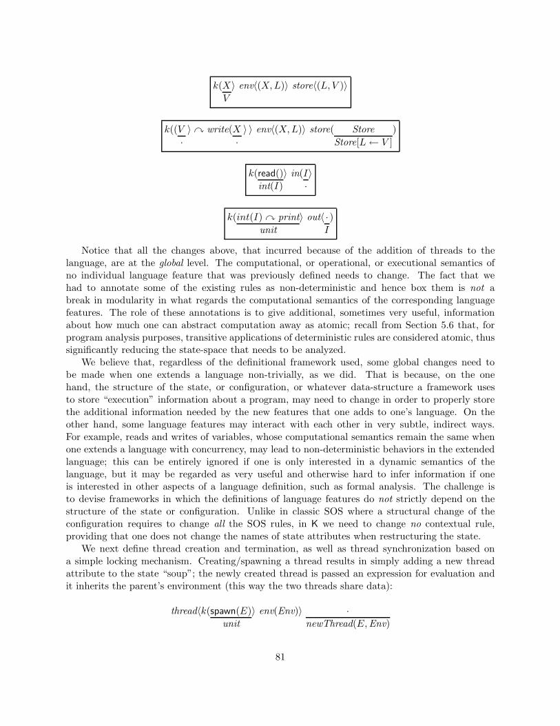
k(XV

〉 env〈(X,L)〉 store〈(L, V )〉

k((V·〉� write(X

·〉 〉 env〈(X,L)〉 store( Store

Store[L← V ])

k(read()int(I)

〉 in(I·〉

k(int(I) � printunit

〉 out〈 ·I

)

Notice that all the changes above, that incurred because of the addition of threads to thelanguage, are at the global level. The computational, or operational, or executional semantics ofno individual language feature that was previously defined needs to change. The fact that wehad to annotate some of the existing rules as non-deterministic and hence box them is not abreak in modularity in what regards the computational semantics of the corresponding languagefeatures. The role of these annotations is to give additional, sometimes very useful, informationabout how much one can abstract computation away as atomic; recall from Section 5.6 that, forprogram analysis purposes, transitive applications of deterministic rules are considered atomic, thussignificantly reducing the state-space that needs to be analyzed.

We believe that, regardless of the definitional framework used, some global changes need tobe made when one extends a language non-trivially, as we did. That is because, on the onehand, the structure of the state, or configuration, or whatever data-structure a framework usesto store “execution” information about a program, may need to change in order to properly storethe additional information needed by the new features that one adds to one’s language. On theother hand, some language features may interact with each other in very subtle, indirect ways.For example, reads and writes of variables, whose computational semantics remain the same whenone extends a language with concurrency, may lead to non-deterministic behaviors in the extendedlanguage; this can be entirely ignored if one is only interested in a dynamic semantics of thelanguage, but it may be regarded as very useful and otherwise hard to infer information if oneis interested in other aspects of a language definition, such as formal analysis. The challenge isto devise frameworks in which the definitions of language features do not strictly depend on thestructure of the state or configuration. Unlike in classic SOS where a structural change of theconfiguration requires to change all the SOS rules, in K we need to change no contextual rule,providing that one does not change the names of state attributes when restructuring the state.

We next define thread creation and termination, as well as thread synchronization based ona simple locking mechanism. Creating/spawning a thread results in simply adding a new threadattribute to the state “soup”; the newly created thread is passed an expression for evaluation andit inherits the parent’s environment (this way the two threads share data):

thread〈k(spawn(E)unit

〉 env(Env)〉 ·newThread(E,Env)

81

When a thread (including the original one) finishes evaluating its expression, it is eliminatedfrom the state releasing all its resources (only locks in our case):

thread〈k( :Val) holds(LCs)〉·

busy( IsIs− LCs

)

Above we assumed an easy to define operation “ − ” that takes a set of integers Is (all thebusy locks) and a set LCs of pairs (lock,counter) and returns the set of locks that are in Is but notin any pair in LCs.

We adopt a simple locking mechanism for thread synchronization, where locks are plain integers.Acquiring a lock requires two cases to analyze, depending upon whether the thread already has thelock or not:

• If the thread already has the lock then “it acquires it once more”, i.e., it increments thecounter associated to that lock:

k(int(I) � acquireunit

〉 holds〈(I, N

s(N))〉

• If the thread does not have the lock and if the lock is available (note that the rule below isconditional) then the thread grabs it and initiates its counter to 0:

k(int(I) � acquireunit

〉 holds〈 ·(I, 0)

〉 busy( IsIs, I

)⇐ not(I in Is)

The condition of the rule above uses an easy to define set membership operation. Also, note that theconditional (computational) rule above is marked as “non-deterministic”. Indeed, the acquisitionof a lock by a thread disables the acquisition of that same lock by other threads “blocking” them,so this action may lead to non-deterministic execution behaviors.

The semantics of release is dual to that of acquire:

k(int(I)) � releaseunit

〉 holds〈(I, s(N)N

)〉

k(int(I) � releaseunit

〉 holds〈(I, 0)·〉 busy〈I

·〉

It is interesting to note that none of the release rules above is non-deterministic. Indeed, therelease of a lock cannot lead to non-deterministic behaviors of multi-threaded programs; in otherwords, if at any moment there are two rules that can be applied, one of them being a release rule,the same behaviors are manifested regardless of which one is chosen.

8.4 Translating MSOS to K

NEXT-VERSION:

82

8.5 Discussion on Modularity

As discussed at the begining of this section, by modularity in the context of programming languagedefinitions it is meant significantly more than just grouping together all the rules corresponding toa particular language feature in a module: a modular framework should allow one to add or removeprogramming language features without a need to modify any of the other, unrelated languagefeatures. Unfortunately, “unrelated language features” is a subtle and hard to rigorously defineconcept; for that reason, it is easy to be interpretable and sometimes misunredstood. We herediscuss, by means of examples, some modularity aspects of language definitional frameworks, how(easily) modularity can be broken, and also how K addresses modularity in language design.

One trivial but fundamental observation about modularity in this context, which makes thedefinition of the concept hard to formalize, is that one would like one’s language design to bemodular without knowing in advance all the other features that will be included in one’s languageeventually. Indeed, when one designs a language, one typically starts small, with a few languageconstructs such as arithmetic expressions, conditional, loops, etc., but then one incrementally addsmore and more complex features, such as functions, recursion, exceptions, etc. If adding a newfeature forces one to revisit and change the definitions of unrelated features that made full sensepreviously, then we say, informally, that one’s design is not modular.

8.5.1 Changes in State Infrastructure

The modularity of many language definitional frameworks is directly affected even by small changesin the structure of the language state infrastructure. Here we assume a rather broad meaningfor “state”: it contains, like in K, everything needed to evaluate a program or a fragment ofprogram, including, besides the program or the fragment of program itself and usual mappings fromvariables to values, also various stacks, resource distribution and availability, messages, signals, etc.Therefore, our generic notion of state here is the same as that of a “configuration” in SOS-baseddefinitional frameworks (assuming that configurations also include all the decorations that someprefer to put as indexes to the reduction relation in SOS definitions, such as those for available“fresh” variables, busy locks, etc.).

Consider, e.g., that one uses a big-step operational semantic style and that one initially has inone’s language only side-effect-free expressions. Then all one needs to do is to define an “evaluationtuple” 〈e, σ〉 ⇓ v that relates expressions e in stores σ to values v, and then devise a standardbig-step derivation system for such tuples by adding “modularly” one or few derivation rules perlanguage construct. However, if one adds now expression constructs that may have side effects, suchas increment (x++) or functions, then one needs to relate (expression,store) configurations to pairscontaining both a value and a new store of the form 〈e, σ〉 ⇓ 〈v, σ′〉, and obviously to change allthe definitions of all the previously defined expression constructs. This simple example shows howeasy it can be for an apparently very natural language definitional framework to be non-modular.

One could say that the above break in modularity appeared because the language designerfailed to consider from the begining an important language design decision: that expressions canhave side effects. While this is arguably true in this simple situation, the same problem reoc-curs frequently during the process of a complex language design. For example, one may later onwant to add language features that will require even more fields in configurations, such as variousstack structures for functions (with return), exceptions, break/continue of loops, etc., as well asrefinements of the existing ones, such as splitting the state into an environment and memory, etc.

83

Each language feature that requires a redisign of the structure of the configuration will enforce thedesigner revisit all the previous language feature definitions and change them to account for thenew configuration structure. Small-step SOS has similar problems, because transitions take placebetween configurations that contain all the needed state infrastructure: changes of the structure ofthe configuration force the redefinition of all or most of the previously defined language features.

Rewriting logic semantics and K avoid the modularity-breaking problems above by allowing thelanguage designer to mention only what is needed from the state infrastructure when defining eachrule. Since equational replacement and term rewriting can take place at any position in a term, notonly at the top of the term as in SOS, the underlying matching mechanism will be responsible forputting each rewrite rule in the “big-context”. For example, to define the semantics of addition,all one needs to do is to state, via rewrite rules, that the evaluation task of an addition expressiondecomposes to the evaluation tasks of its two subexpressions which are placed at the top of thecontinuation structure, and then the results, when and if they are eventually produced on the topof the continuation replacing the original subexpressions, are combined into a result of the additionexpression. No other state infastructure except the addition expression itself is mentioned in therules, so future changes of the state structure to accomodate additional language features will notaffect the current definition of addition.

In addition to the increase in modularity obtained by adopting a rewriting logic semantics style,K provides, through its context transformers, additional increases in modularity by automaticallyupdating all the rules when the state infrastructure changes invalidate the well-formedness of rules.

8.5.2 Control-Intensive Language Constructs

Another important factor which adversarily affects the modularity of many existing language defini-tional approaches, is the control-intensive nature of several interesting and useful modern program-ming language constructs, such as the different types of exceptions. By control-intensive constructswe here mean ones which may change the control execution flow of the program abruptly, forcingthe execution of the program to discard its current environment and control information (such asfunction stack frames, exception stacks, etc.), replacing them by others, for example, ones whichwere previously encountered and “saved”.

Language definitional frameworks in which the derivation of an expression cannot continue un-less (some or all of) its subexpressions are first derived, such as, for example, the SOS definitionalstyles, suffer the most in what regards modularity when one adds control-intensive language con-structs to ones language. That is because the semantics of control-intensive constructs do not followthe discipline and modularity of traditional mathematical logic reasoning, in particular, derivationtasks (or proofs) that are started need not terminate. For example, the evaluation of E1 in anexpression E1 + E2 may throw an exception, in which case the “control” will be never given backto the addition to complete its semantic definition. Control-intensive statements are not impos-sible to define in SOS-like frameworks, but their definitions look awkward and lose the intendedcomputation granularity of the defined statements.

Consider, for example, the addition of a halt construct to a language, that takes an expression,evaluates it to a value, and then stops the execution of the entire program with that value as aresult. A halt can appear anywhere in the program, so one should be able to discard the “remaining”computation instantly from any evaluation context. In a big-step semantic framework, one wouldneed to add a special “value”, say halt(v), and then add for each language construct as many rulesas subexpressions or substatements that construct has that can generate a halt signal. This break

84

of modularity is not only a practical inconvenience for the language designer because it more thandoubles the number of derivation rules in ones language definition, but it does not scale either.Consider now also adding parametric exceptions, return to functions, break/continue to loops, etc.Each of these will more than double again the number of rules, not to mention that they mayinterfere in rather unexpected ways.

Moreover, from a computational granularity perspective, big-step and/or small-step SOS def-initions of control-intensive statements such as halt are not entirely correct: they fail to capturethe intended computational granularity of these statements, which, like their functional behavior,is an important component of their formal semantics. Indeed, the intended semantics of halt(E) is“evaluate E to a value V and then return V as the result of the entire program”; compare that with“evaluate E to a value V and then propagate a halting signal with V through all the remainingstatements until none left and then return V as the result of the entire program”, which is howhalt is defined in big-step or small-step SOS.

As already seen in previous sections, control-intensive statements present no difficulty in K. Likein context reduction or other continuation-based approaches, in K we maintain the control of theprogram explicit as part of the state infrastructure, so contextual rules defining the semantics ofcontrol-intensive constructs can easily store, remove or modify the control context of the program.This allows for an increased modularity of language definitions, because no “propagation” rulesof control-changing signals are needed; in particular, as shown at the botom of Figure 2 the K-semantics of halt consists of precisely one rule, which stops the program with the desired value inone computational step, exactly as expected.

8.5.3 On Orthogonality of Language Features

Let us now discuss in more depth the subtle issue of when two or more language features are “un-related” or orthogonal, which is the criterion that we use informally to characterize the modularityof language definitional frameworks: a framework is modular when the addition of a new languageconstruct does not require one to modify the definition of any of the existing, “unrelated” lan-guage features. At one extreme, one could say that programming languages are monolithic, in thesense that any feature is related to any other feature in the language, in which case the concept ofmodularity is superfluous because any definition of the language in any framework is modular.

At another extreme, one could say that all language features should be orthogonal to eachother, in which case modularity becomes again a non-issue because no open-ended language designcan be modular: one can always add features to a language that interact in previously unexpectedways with other features. For example, one can add dynamic aspects to an otherwise pure object-oriented programming language, in which case additional code may need to be executed whencertain events take place, such as, e.g., returns from method calls or updates of values storedat particular locations. Another common example would be the addition of concurrency to alanguage whose functions are allowed to terminate abruptly with return statemens; if one decidesthat all locks acquired during the execution of a function should be automatically released when thefunction is terminated with a return (which is actually a “must” if locks are acquired and releasedvia “synchronized (Lock) {Code}” blocks, like in Java), then the previous definition of the functioncall originally designed for a sequential language is not orthogonal to the addition of concurrencyand locks: indeed, it needs to be changed to account for the release of the locks accumulated sincethe function was called.

We believe that the related notions of orthogonality and modularity of language features are

85

closely coupled with several factors, including at least the following:

1. the particular programming language paradigm underlying one’s language;

2. the particular definitional framework that ones is employing;

3. the particular definitional methodology that one uses within one’s definitional framework;

4. the restrictions that one imposes on languages defined using one’s approach and methodology.

For example, regarding the first item, a pattern matching has different meanings and interactionswith the rest of the language features in functional languages, versus in logic programming lan-guages, versus in term-rewrite languages using rewrite strategies. Even simple language constructs,for example an addition “E1 + E2”, can have different meanings in languages obeying differentparadigms: functional and imperative languages evaluate E1 and E2 to values in the current ex-ecution environment and then calculate the sum of the two values, logic programming languagesmay use the variables in E1 and E2 for unification purposes, (pure) object oriented languages in-terpret addition as a unary method call “E1. + (E2)” or message send “send E1 message + (E2)”,etc. In other words, regardless of the particular definitional framework that one uses to defineprogramming languages, in general one cannot simply take a definition of a language constructfor a particular language paradigm, and expect to use it “as is” for a language following a dif-ferent language paradigm. Moreover, even within one language paradigm, the addition of futurefeatures may non-trivially colide with the meaning of existing language features. For example, in aside-effect-free imperative programming language one may give addition a “parallel” semantics: toevaluate “E1 + E2”, evaluate E1 and E2 in parallel and then sum their values. However, the addi-tion of side effects to the language make the existing definition of addition have a non-deterministicbehavior, which may be undesirable; if this is the case, then one needs to revisit the definition ofaddition and “sequentialize” it, thus resulting in a break of modularity.

Regarding the second item, if one employs for example SOS as a definitional framework, thenone may argue that the halt statement in particular and exceptions in general are not orthogonalto the other statements of the language, simply because halt or throwing an exception can abruptlychange the behavior of the other statements, “as faithfully captured by their SOS definitions”. Aswe have seen in the various K definitions in this paper, halt and exceptions are orthogonal withother language features when one employs a different language definitional approach. Therefore,the orthogonality or the lack of orthogonality of a particular language feature is relative to thedefinitional framework that is being used. Informally, and certainly not conclusively, we say that adefinitional framework is more modular than another framework for a given programming language,when the former has fewer rules (directly or indirectly) refering to more than one language constructthan the latter.

With respect to the third item, it is important to realize that it does not suffice to use a particulardefinitional framework in order to guarantee modularity. For example, one can use rewriting logicas a framework to develope big-step or small-step SOS definitions of languages as shown in Section4, and then one’s definitions will be as modular as SOS.

Regarding the fourth item, one can indeed easily claim the modularity of a (perhaps any) frame-work or methodology when one disallows “inconvenient” language features, such as, for example,parametric exceptions, concurrency, call/cc, etc.

We next discuss several instances in which modularity of definitions of language features hasbeen broken in our definitions of programming languages using K, in other words, situations in

86

which we realized that our previously defined language features need to be reviseted and changedwhen we wanted to add other language features.

Functions with Return. We initially had no plans for adding a return construct to FUNfor abrupt return from function calls. Therefore, our previous semantics of function invocationconsisted of just binding the closure parameters to the actual arguments in the closure environment,then evaluate the body of the function just like any other expression, and then recover only thecallee environment when a value was produced; no function stack was needed. The addition ofreturn forced us to change the previous definition of function invocation, by adding a function stackin which environment and control information needed to recover the callee evaluation context incase of abrupt return needs to be stored. Besides abrupt function termination using return, forwhich we obviously had to provide a contextual rule, we decided to also allow normal functiontermination, without return, so we had to modify the previous rule for function call terminationto account for the new function stack structure. An alternative language design decision couldhave been to assume that all functions have an ending return, even to enforce that by a simplecode transformation, in which case the previous rule for function call termination could have beenentirely eliminated.

Break/Continue of Loops. Loops without break and continue are straightforward to give asemantics in any operational framework. Originally, like with the return of functions, we had noplan for adding break and continue to FUN, so we defined the semantics of while loops following theusual (small-step) approach, namely by translating them into a conditional checking the conditionof the loop and, if true, executing the body of the loop followed by the loop. Moreover, since weknew no language that has for loops but does not have while loops, we translated all for loops intocorresponding while loops. We believe that these are common reasonable design decisions for thesemantics of loops. However, the addition of break and continue made us change completeley ourdefinitions for loops, as follows:

1. Since break and continue act as exceptions, in the sense that they switch the execution contextto one that has been encountered “back in time”, and since loops can be nested, we had toadd a new stack in the control component of the state infrastructure, dedicated to loops,which would keep all the information needed to recover the computation context in case of abreak or continue;

2. Loops cannot be given a semantics via a simple unrolling anymore, because one needs topop the loop stack when the loop is terminated; therefore, we had to change the previousdefinition based on unrollings of the loop;

3. Interestingly, in the presence of continue, one cannot even translate a for loop into a while loop,because that would not be semantically correct: unlike in a while loop where one needs toonly jump to the next iteration recovering the computation context appropriately, a continueof a for loop additionally executes the step update of the loop, typically an increment or adecrement of a counter variable. It turns out that it is actually more convenient to translatewhile loops into particular for loops, namely ones without step statements, and then only givethe semantics of the latter. This twist was entirely unexpected to us originally.

87

Another interesting and originally unexpected side effect of adding break and continue to loops,was that they are not entirely orthogonal to function calls, either! Imagine a program wherea function is called from inside a loop and that the evaluation of that function encounters noloops but does encounter a break or a continue. In the current definition of FUN in Section 6, wedeliberately decided to do nothing about stopping such executions dynamically: such a break orcontinue would act quite like an exception that crosses the bounderies of function calls, that is,it would break or continue the loop from which the function was invoked. Such an unrestrictedprogramming language behavior may admitedly be considered strange, even unacceptable, by mostlanguage designers (including the author), but there may also be some designers who like it. It isnot the task of designers of language design frameworks to decide what a language designer shouldlike or not in her language, but to develop frameworks that allow one to define any programminglanguage with any desired features, be they strange or not.

There are at least two ways to address such violations of orthogonality of language features. Oneis to admit that the involved features are not orthogonal, and thus to change the semantics of oneof them or of both to account for their possibly desired interaction. In our definition of FUN, in thiscase we would need to change the semantics of function invocations as follows: together with theother ingredients pushed in the function stack when an invocation takes place, also push the currentloop stack and then empty it before the control is passed to the function body; then recover theloop stack at return from the function call. This way, a break or continue “thrown” by the functionthat is not properly “caught” by a loop defined in the function body will stuck the execution ofthe program (or one can throw some appropriate exception, if one likes it that way). Anotherpossibility, commonly adopted in existing programming languages and also assumed by the currentdefinition of FUN, is to dissalow programs potentially violating the orthogonality of features. Inour case, for example, this can be done by using a simple static checker that would reject functionscontaining break or continue that are not enclosed by loops defined inside the function.

To summarize the discussion above, we believe that modularity and orthogonality of program-ming language features are subtle notions that depend on many factors, which appear to be hardto formally define and investigate in a generic, rather than programming language specific, way.

88

9 On Language Semantics

NEXT-VERSION:

9.1 Initial Algebra Semantics Revisited

NEXT-VERSION:

9.2 Initial Model Semantics in Rewriting Logic

NEXT-VERSION:

89

10 On Formal Analysis

In this section we show how one can use the rewrite logic definition of a language to formallyanalyze programs. This is achieved by using generic executability or analysis tools for rewritinglogic. The formal analyses discussed in this section fall into the following categories: static typechecking and type inference, type preservation and progress, concurrency analysis (e.g., dataracesand deadlocks), and model checking.

To illustrate our rewrite-based techniques for type checking, type inference, as well as for provingproperties about or in connection to types, in this section and in Section 10.3 we assume thesimplified version of the FUN language in Figure 10, without any control intensive features. Wewill define a type system for this language encoding a common typing policy. Note that here we donot consider types to be part of the language; they are nothing but an abstraction of the program,useful for static analysis purposes, to reject or warn about programs that are considered to bebadly written. There are also languages in which types form an important part of the languagesemantics, playing a “dynamic” role in the execution of programs, that is, programs may manifestdifferent behaviors depending upon the runtime types of some of its expressions; such a languageis for example KOOL, defined in Section 7. If that is the case, then one should define types as partof the language semantics, as we did in Section 7.

10.1 Type Checking

There was little in the definition of our functional programming language so far which would forbidone from writing erroneous programs. While the domain or application specific errors are hard orimpossible to catch automatically, there is a large class of errors, known as type errors, which oftencan be caught automatically with appropriate program analysis tools.

Static type checkers are special program analysis tools that take programs as inputs and reporttype errors, which may turn into runtime errors or misbehaviors. Type checkers are so popularnowadays and the kind of errors they catch so frequently lead to wrong behaviors, that mostcompilers today provide a static type checking analysis tool as a front end. The major drawback ofstatic type checkers is that they may reject correct programs, so they somehow limit the possibilitiesof writing programs.

Typed Languages

A typed language defines a set of types, as well as a typing policy by which types can be associatedto values calculated by programs.

By applying the typing policy recursively, one can mechanically associate a type to each ex-pression in a given program. In order to do it, one needs to inspect the invocations of languageconstructs and check that each language construct is used properly by analyzing the relationshipbetween its operands, their expected types and the context in which the language construct appears.

If a language construct use is found to violate the expected typing policies, then we say that atype error has been found. E.g., think of the expression 3 + (fun x -> x). While under certainspecial circumstances one may wish to accept such programs as correct, in general a typing policywould classify this is as a type error.

When designing a type checking tool for a typed language, one needs to take a decision on whatto do when a type error is found.

90

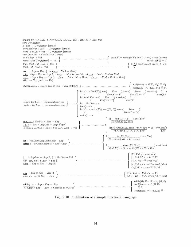
import VARIABLE, LOCATION, BOOL, INT, REAL, K[Exp,Val]sort ConfigItemk :Exp→ ConfigItem [struct]env : Set[Var � Loc]→ ConfigItem [struct]store :Set[Loc � Val]→ ConfigItem [struct]nextLoc : Int→ ConfigItem [struct]eval :Exp→ Valresult : Set[ConfigItem]→ Val

ff. . . . . . . . . . . . . . . . . . . . . . . . . . . . . . . . . . . . . . .

jeval(E) = result(k(E) env(·) store(·) nextLoc(0))

result〈k(V )〉 = V

Var, Bool, Int, Real < ExpBool, Int, Real < Val

ff. . . . . . . . . . . . . . . . . . . . . . . . . . . . . . . . . . . . . . . . . . . . . . . . . . . . . . . . . . .

jk(X

V〉 env〈(X, L)〉 store〈(L, V )〉

not : Exp→ Exp [!, notBool : Bool → Bool ]+ :Exp× Exp→ Exp [!, +Int : Int× Int→ Int, +Real :Real ×Real→ Real]≤ : Exp × Exp→ Exp [!, ≤Int : Int× Int→ Bool, ≤Real : Real× Real→ Bool]

skip :→ Exp [unit :→ Val]

if then else : Exp× Exp× Exp→ Exp [!(1)[if]]¯

. . . . . . . . . . . . . . . . . . . . . . . . . . . . . . . . . . . . . . . .

(bool(true) � if(E1, E2)

→= E1

bool(false) � if(E1, E2)→= E2

bind : VarList→ ComputationItemwrite : VarList→ ComputationItem

ff. . . . .

8>>>>>>>>>>>><>>>>>>>>>>>>:

k((V·〉� bind(X

·〉〉 env( Env

Env[X ← L]) store( Store

Store[L← V ]) nextLoc( L

next(L))

k((bind(X·〉〉 env( Env

Env[X ← L]) nextLoc( L

next(L))

k(· : ValList〉 = ·bind(·) = ·k((V·〉� write(X

·〉〉 env〈(X, L)〉 store( Store

Store[L← V ])

write(·) = ·

fun → :VarList× Exp→ Exp( ) : Exp× ExpList→ Exp [![app]]

closure :VarList× Exp × Set[Var � Loc]→ Val

9=; . . . . . . . . . . . . . . . . . . .

8>>>><>>>>:

k( fun Xl→ Eclosure(Xl, E,Env)

〉 env(Env)

k((closure(Xl, E,Env), Vl) � appVl � bind(Xl) � E � Env′

� K) env(Env′Env

)

let : VarList×ExpList×Exp→Expletrec : VarList×ExpList×Exp→Exp

ff. . . . . . . . . . . . . . . . . . . . . . . . . .

8>>>><>>>>:

k( let(Xl, El, E)El � bind(Xl) � E � Env

〉 env(Env)

k( letrec(Xl,El, E)bind(Xl) � El � write(Xl) � E � Env

〉 env(Env)

[ ] : ExpList→ Exp [!, [ ] : ValList→ Val]

car, cdr, null? : Exp→ Exp [!]cons : Exp× Exp→ Exp [!]

9=; . . . . . . . . . . . . . . . . . . . . . . . . . . . . . . . . . . . . . . . . . .

8>>>>><>>>>>:

[V :Val, ] � car→= V

[ :Val, Vl] � cdr→= Vl

[·] � null?→= bool(true)

[ :Val, ] � null?→= bool(false)

(V, [Vl]) � cons→= [V,Vl]

; : Exp× Exp→ Exp [!]:= : Var× Exp→ Exp

ff. . . . . . . . . . . . . . . . . . . . . . . . . . . . . . . . . . . . . . . . . . . . . . . . . . . . . . .

j(V1 :Val, V2 :Val) � ; = V2

(X := E) = E � write(X) � unit

while( ) : Exp× Exp→ Exp

� :Exp × Exp→ Exp→ ContinuationItem

ff. . . . . . . . . . . . . . . . . . . . . . . . . . . . . . . . . . . . . . . . . . . . . .

8>><>>:

while(B) E = B � � (B,E)bool (true)

E; B� � (B,E)

bool (false) � � (B,E)→= ·

Figure 10: K definition of a simple functional language

91

The simplest decision is to reject the program. Better decisions are to also report where theerror has been found, as well as possible causes, to users. Even better, the type checker can continueand report subsequent type errors within only one session.

One can even think of taking automatically some correcting measures, such as to convert integersto reals, or kilometers to miles, or to modify the code by introducing runtime checks, etc.

Dynamic Type Checking

At the expense of increasing their runtime overhead, some languages maintain a type togetherwith each computed value in their store. This way, variables are associated not only values butalso the types of those values. Before an operation is applied, a dynamic type checker validatesthe application of the operation. In the case of 3 + (fun x -> x), before the operation + isevaluated the dynamic type checker checks whether the two operands are integers; this way aruntime error will be reported.

While dynamic type checking is useful and precise, and many successful programming languagesare dynamically typed, such as Scheme, PERL, Python, etc., many programming language designersbelieve that runtime checks are too expensive in practice.

Untyped Memory Models

If one simply removes the runtime checks for type consistency then one can obviously run intoserious difficulties. For example, when adding an integer and a function, since they are both storedas binary numbers at some locations, without a consistency check one would just add the integerwith the binary representation of (part of) a particular representation of the function, which iswrong.

Languages without runtime or dynamic type checking are said to have untyped memory models.Such languages essentially assume that the operations are applied on the right data, so they canincrease their performance by removing the runtime type consistency checks.

Static Type Checking

To take full advantage of the increased execution speed of untyped memory models while still notsacrificing the correct runtime behavior of programs, an additional layer of certification is needed.More precisely, one needs to ensure before execution that all the operations will be applied on theexpected type of data. This process is known under the terminology static type checking.

Languages admitting static type checkers, that ensure that once a program passes the typechecker it will never exhibit any type error at runtime, are called strongly statically typed. It isquite hard or even impossible (due to undecidability arguments) in practice to devise strongly typedlanguages where the types are intended to state that a program is free of general purpose errors.For example, it is known to be undecidable to say whether a program will ever perform a divisionby zero, or if a program terminates.

To keep static type checkers decidable and tractable, one typically has to restrict the class oferrors that types can exhibit. In the context of our simple functional programming language, likein many other languages, by a type error we mean one of the following:

• An application of a non-functional expression to an argument;

92

• An application of a function expression to arguments whose types are different from those offunction’s parameters;

• An assignment of an expression to an existing name, such that the type of the expression isdifferent from the declared type of the name;

• A use of an arithmetic or boolean operation on non-integers or non-booleans, respectively;

• A use of a conditional statement where the first argument is not a boolean or where the twobranches are of different type.

Besides the simplistic typing policy above, we also need to state how the types of expressionsare calculated and propagated via typing rules. For example, “the type of x + y is int if the typesof x and y are int”. Similarly, “the type of a conditional is the type of its first branch if the typeof its argument is bool and the types of its branches coincide”.

In order to allow type checking in a language, one first needs to extend the language with typedeclarations, so that one can add typing information to the program. We will see later, when wediscuss type inference, that in some situations types can be deduced automatically by examininghow names and expressions are used.

Since declarations can occur either in a let/letrec statement or in a function (its parameter),we will slightly extend the syntax of our language to allow type declarations in addition to and atthe same time with name declarations. For example, we will allow expressions like

let int x = 17 in xlet int x = 17 and int y = 10 in x + y

Besides the basic types int and bool, we will also introduce several other types and typeconstructors. Since our language is functional we will need to introduce function types, using thecommon type constructor -> . Thus, we will be able to write and type-check expressions like

let int a = 3in let (int -> int) p = fun(int x) -> x + a

and int a = 5in a * p(2)

Note that, by design, we decided to first place the type of a parameter and then its name. Asbefore, we also assume that the default calling mode is call-by-value. So expressions like the onebelow will also type check (note also the tricky typing of letrec):

letrec int x = 2and ((int,int) -> int) f = fun (int y, int z) -> y + x * zin f(1,x)

As seen in Figure 10, to simplify the semantic definition of the language we assumed that all thetypes in a type declaration are grouped together in a list that is given as an additional argumentto the corresponding language construct. It is straightforward to automatically transform theprograms in this spirit (see the provided Maude code).

93

Defining Program Analysis Tools

The modular design of our programming language was intended not only to easily deal with changesin the design of the language, but also to facilitate the definition of program analysis tools.

In fact, the definition of a program analysis tool can be seen as very similar in spirit to defininga semantics to a programming language. The meaning a program analysis tool has for a programmay, of course, be quite different from that of the semantics of the programming language, becausethe two may look at two quite different aspects of a program.

However, we will again take advantage of the efficient executable environment provided byMaude through its fast implementation of rewriting, and this way obtain not only executable butalso quite efficient program analysis tools for free, from just their mathematical rigorous definition.

A Big-Step Definition of a Type Checker

As we saw at the begining of the class, big-step semantics are simpler and more efficiently exe-cutable than other semantics when they work. There were two problems making big-step semanticsinappropriate: concurrency and control-intensive statements. Since we have none of these problemswhen we define a type-checker for our language, a big-step semantics is appropriate in this case.

Adding Types to the Syntax

There are very few changes that need to be done to the syntax of our functional programminglanguage in order to allow type declarations. First, of course, one has to introduce the types:

fmod TYPE issorts Type TypeList .subsort Type < TypeList .op nil : -> TypeList .op _,_ : TypeList TypeList -> TypeList [assoc id: nil] .ops int bool none : -> Type .op _->_ : TypeList Type -> Type [gather(e E)] .op list_ : Type -> Type [prec 0] .

endfm

Besides bool and int, note that there is one more basic type, none, which will be the type ofexpressions that are supposed to evaluate to unit (assignments, loops, etc.). We also define lists oftypes, for two reasons: (1) the type of the argument of a function is a list of types (an alternativewould have been to introduce product types for the same purpose; in fact, one can think of lists oftypes as product types), and (2) as usual, we prefer to process expressions in bulk, so typing a listof expressions results in a list of types.

The type of a function without parameters returning an integer will be therefore nil -> int.To avoid writing parentheses, note that the function type constructor, -> has been defined asright-associative. Note that this is opposite to the definition of function application, which wasdefined left-associative, and that these two conventions are consistent.

The language constructs that declare variables, i.e., functions, let and letrec, need to be changedto assign a type to each declared variable. To simplify our semantics later, we prefer to declare thetypes of all the corresponding variables in a list:

94

op fun__->_ : TypeList NameList Exp -> Exp ....op let : TypeList NameList ExpList Exp -> Exp .

...op letrec : TypeList NameList ExpList Exp -> Exp .

No other changes are needed to the syntax of the language. As already mentioned, one caneasily transform the code to offer the user a nicer language interface, where each variable is prefixedwith its type (see the provided file fun-type-checking-semantics.maude, which is also explainedbelow).

Defining a Static Type Checker

The general idea underlying a static type checker is to recursively analyze each language constructoccurring in a given program, to chack that its operands satisfy the type constraints, and then toassign a type to the expression created by that new construct.

The type of a name cannot be changed by variable assignment constructs, so a name has itsdeclared type in all its occurrences within its scope; but clearly one can differentiate between staticand dynamic scoping. We will only consider static scoping.

Exercise 1 (Very hard!). Define a static type checker for the dynamically scoped version of FUN.Can the task be accomplished precisely? If not, choose some acceptable trade-offs so that the typechecker stays reasonably efficient.

Defining the State Infrastructure

Any software analysis tool has a configuration or state that it maintains as it traverses the programto be analyzed. This is also what happened in the definition of the semantics of the language.In fact, there is a striking similarity in giving various executable semantics to a given syntax:a programming language semantics is just one possibility; a type checker is another one; othersoftware analysis tools can be defined similarly, including complex type systems or abstractions.

A type checker ignores the concrete values bound to names, but it needs instead to bind namesto their types. We can realize that by defining a special state attribute, called TypeEnv, whichcontains a mapping from names to their current types. In order to do define this module, weneed to first define lists of names and of types. The former were already defined in the seman-tics of FUN, and the latter are similar, so we do not discuss them here. See the provided filefun-type-checking-semantics.maude for the complete Maude specification of the static typechecker discussed here.

The following module can simply “cut-and-paste” the module ENVIRONMENT defined by theexecutable semantics of FUN; however, one needs to replace locations by types. One can also useMaude’s parameterized modules, but we do not do it here.

fmod TYPE-ENVIRONMENT isprotecting NAME-LIST .protecting TYPE .sort TypeEnv .op empty : -> TypeEnv .op [_,_] : Name Type -> TypeEnv .

95

op __ : TypeEnv TypeEnv -> TypeEnv [assoc comm id: empty] .op _[_] : TypeEnv Name -> [Type] .op _[_<-_] : TypeEnv NameList TypeList -> TypeEnv .var X : Name . vars TEnv : TypeEnv . vars T T’ : Type .var Xl : NameList . var Tl : TypeList .eq ([X,T] TEnv)[X] = T .eq TEnv[nil <- nil] = TEnv .eq ([X,T] TEnv)[X,Xl <- T’,Tl] = ([X,T’] TEnv)[Xl <- Tl] .eq TEnv[X,Xl <- T,Tl] = (TEnv [X,T])[Xl <- Tl] [owise] .

endfm

In this case, no other information but the type environment is needed by the static type checker.However, to preserve our general semantic definition methodology, we prefer to define a state ofthe type checker which contains only one state attribute for the time being, the type environment.Extensions of the language may require new state attributes in the future:

fmod TYPE-STATE isextending TYPE-ENVIRONMENT .sorts TypeStateAttribute TypeState .subsort TypeStateAttribute < TypeState .op empty : -> TypeState .op __ : TypeState TypeState -> TypeState [assoc comm id: empty] .op tenv : TypeEnv -> TypeStateAttribute .

endfm

We can now finalize the state infrastructure by defining the following module, which, like forthe semantics of the language, provides an abstract state interface for the subsequent modules:

fmod HELPING-OPERATIONS isprotecting GENERIC-EXP-LIST-SYNTAX .protecting TYPE-STATE .op initialTypeState : -> TypeState .op _[_] : TypeState Name -> [Type] .op _[_<-_] : TypeState NameList TypeList -> TypeState .var S : TypeState . var TEnv : TypeEnv .var X : Name . var Xl : NameList . var Tl : TypeList .eq initialTypeState = tenv(empty) .eq (tenv(TEnv) S)[X] = TEnv[X] .eq (tenv(TEnv) S)[Xl <- Tl] = tenv(TEnv[Xl <- Tl]) S .

endfm

S[X] gives the type associated to a name X in a state S, while S[Xl <- Tl] updates the typesof the names in the list Xl to Tl.

Typing Generic Expressions

Like in the case of the semantic definition of FUN, we need to “evaluate” an expression to a “value”.However, this time, the values that expressions evaluated to are types. Unlike in the definition ofthe semantics of the language where side effects could modify the values bound to names, the typebound to a name cannot be modified.

96

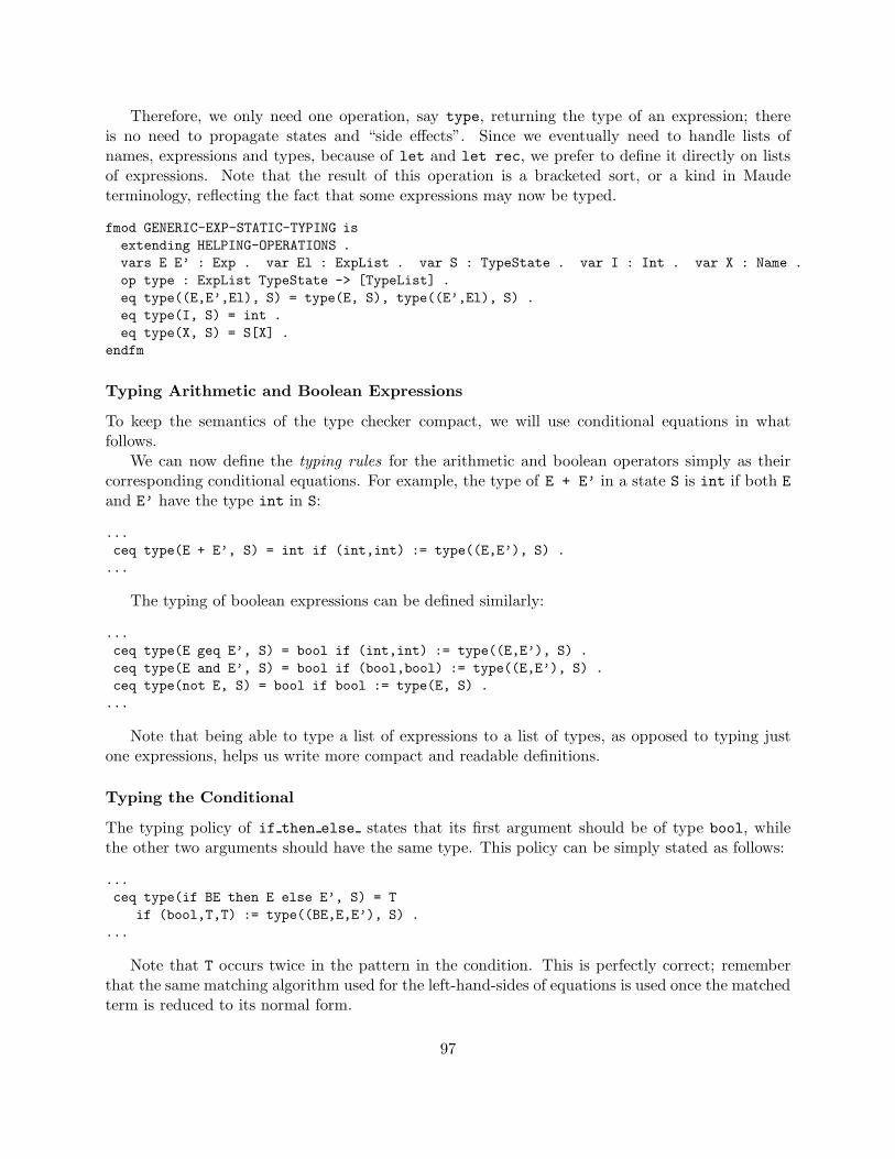
Therefore, we only need one operation, say type, returning the type of an expression; thereis no need to propagate states and “side effects”. Since we eventually need to handle lists ofnames, expressions and types, because of let and let rec, we prefer to define it directly on listsof expressions. Note that the result of this operation is a bracketed sort, or a kind in Maudeterminology, reflecting the fact that some expressions may now be typed.

fmod GENERIC-EXP-STATIC-TYPING isextending HELPING-OPERATIONS .vars E E’ : Exp . var El : ExpList . var S : TypeState . var I : Int . var X : Name .op type : ExpList TypeState -> [TypeList] .eq type((E,E’,El), S) = type(E, S), type((E’,El), S) .eq type(I, S) = int .eq type(X, S) = S[X] .

endfm

Typing Arithmetic and Boolean Expressions

To keep the semantics of the type checker compact, we will use conditional equations in whatfollows.

We can now define the typing rules for the arithmetic and boolean operators simply as theircorresponding conditional equations. For example, the type of E + E’ in a state S is int if both Eand E’ have the type int in S:

...ceq type(E + E’, S) = int if (int,int) := type((E,E’), S) .

...

The typing of boolean expressions can be defined similarly:

...ceq type(E geq E’, S) = bool if (int,int) := type((E,E’), S) .ceq type(E and E’, S) = bool if (bool,bool) := type((E,E’), S) .ceq type(not E, S) = bool if bool := type(E, S) .

...

Note that being able to type a list of expressions to a list of types, as opposed to typing justone expressions, helps us write more compact and readable definitions.

Typing the Conditional

The typing policy of if then else states that its first argument should be of type bool, whilethe other two arguments should have the same type. This policy can be simply stated as follows:

...ceq type(if BE then E else E’, S) = T

if (bool,T,T) := type((BE,E,E’), S) ....

Note that T occurs twice in the pattern in the condition. This is perfectly correct; rememberthat the same matching algorithm used for the left-hand-sides of equations is used once the matchedterm is reduced to its normal form.

97

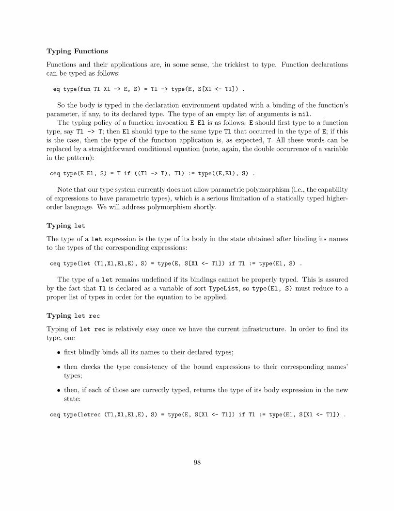
Typing Functions

Functions and their applications are, in some sense, the trickiest to type. Function declarationscan be typed as follows:

eq type(fun Tl Xl -> E, S) = Tl -> type(E, S[Xl <- Tl]) .

So the body is typed in the declaration environment updated with a binding of the function’sparameter, if any, to its declared type. The type of an empty list of arguments is nil.

The typing policy of a function invocation E El is as follows: E should first type to a functiontype, say Tl -> T; then El should type to the same type Tl that occurred in the type of E; if thisis the case, then the type of the function application is, as expected, T. All these words can bereplaced by a straightforward conditional equation (note, again, the double occurrence of a variablein the pattern):

ceq type(E El, S) = T if ((Tl -> T), Tl) := type((E,El), S) .

Note that our type system currently does not allow parametric polymorphism (i.e., the capabilityof expressions to have parametric types), which is a serious limitation of a statically typed higher-order language. We will address polymorphism shortly.

Typing let

The type of a let expression is the type of its body in the state obtained after binding its namesto the types of the corresponding expressions:

ceq type(let (Tl,Xl,El,E), S) = type(E, S[Xl <- Tl]) if Tl := type(El, S) .

The type of a let remains undefined if its bindings cannot be properly typed. This is assuredby the fact that Tl is declared as a variable of sort TypeList, so type(El, S) must reduce to aproper list of types in order for the equation to be applied.

Typing let rec

Typing of let rec is relatively easy once we have the current infrastructure. In order to find itstype, one

• first blindly binds all its names to their declared types;

• then checks the type consistency of the bound expressions to their corresponding names’types;

• then, if each of those are correctly typed, returns the type of its body expression in the newstate:

ceq type(letrec (Tl,Xl,El,E), S) = type(E, S[Xl <- Tl]) if Tl := type(El, S[Xl <- Tl]) .

98

Typing Lists

The typing policy of lists is that each element in the list should have the same type, say T; if thisis the case, then the type of the list expression is list T. For example, [1 :: 2 :: 3] is typed tolist int, while [1 :: true :: 3] generates a type error.

How about the type of the empty list, [nil]? It must be a list of some type, but what type?This is a subtle problem, related, again, to polymorphism. We will discuss polymorphism shortly.For now, to keep our language type-checkable, we make the strong and admittedly unsatisfactoryassumption that all empty lists have type list int. Hence, we need an operator that takes anExpList and returns the type of its elements. With that, the type of a list can be simply definedas follows:

op collapseType : TypeList -> Type .eq collapseType(nil) = int .eq collapseType(T,T,Tl) = collapseType(T,Tl) .ceq type([El], S) = list T if T := collapseType(type(El, S)) .

The typing rules of the list operations are self-explanatory:

ceq type(car(E), S) = T if list T := type(E, S) .ceq type(cdr(E), S) = list T if list T := type(E, S) .ceq type(cons(E,E’), S) = list T if (T, list T) := type((E,E’), S) .ceq type(null?(E), S) = bool if list T := type(E, S) .

Typing Assignment and Sequential Composition

A variable assignment statement should not modify the type of the name on which it applies itsside effect. Also, since we decided to evaluate assignment statements to the value nothing, wealso type them to the special type none, so the type system will signal if one uses them in wrongcontexts, for example as integers:

ceq type(X := E, S) = none if type(X, S) = type(E, S) .

The type of E ; E’ is the type of E’, but only if E also can be correctly typed, say to sometype T:

ceq type(E ; E’, S) = T’ if (T, T’) := type((E,E’), S) .

Typing Loops

Loops type check as follows:

ceq type(while Cond Body, S) = noneif (bool,T) := type((Cond, Body), S) .

Note that the type of a loop is none only if its condition types to bool and its body to someproper type. We could have just as well required that the type of its body be none, or that thetype of the loop is the type of its body, etc.

99

Putting the Type Checker Together

Like in the semantics of FUN, we can now put everything together by defining one unifying moduleimporting all the various features. This module also defines an operation that can check andcalculate the type of an expression in the initial state:

op type : Exp -> [Type] .eq type(E) = type(E, initialTypeState) .

For writing programs in a more human readable way, we can also define now some sytacticsugar notations:

--- some syntactic sugar--- for bindingssorts Binding Bindings .subsort Binding < Bindings .op __=_ : Type Name Exp -> Binding .op (_,_,_) : TypeList NameList ExpList -> Binding .op nil : -> Bindings .op _and_ : Bindings Bindings -> Bindings [assoc id: nil prec 100] .ops (let_in_) (letrec_in_) : Bindings Exp -> Exp .var T : Type . var X : Name . vars Tl Tl’ : TypeList .vars Xl Xl’ : NameList . vars El El’ : ExpList .eq (T X = E) = (T,X,E) .eq (Tl,Xl,El) and (Tl’,Xl’,El’) = ((Tl,Tl’), (Xl,Xl’), (El,El’)) .eq let (Tl,Xl,El) in E = let(Tl,Xl,El,E) .eq letrec (Tl,Xl,El) in E = letrec(Tl,Xl,El,E) .

--- for functionssorts Parameter ParameterList .subsort Parameter < ParameterList .op __ : Type Name -> Parameter [prec 0] .op ‘(‘) : -> ParameterList .op _,_ : ParameterList ParameterList -> ParameterList [assoc id: ()] .op (_,_) : TypeList NameList -> ParameterList .op fun_->_ : ParameterList Exp -> Exp .eq () = (nil,nil) .eq T X = (T,X) .eq (Tl,Xl),(Tl’,Xl’) = ((Tl,Tl’),(Xl,Xl’)) .eq fun (Tl,Xl) -> E = fun__->_(Tl,Xl,E) .

Polymorphism

Let us consider a “projection” function fun (x,y) -> x which takes two arguments and alwaysreturns its first argument. In the context of our typed language above where the user is expected toassign a type to each declared variable, one is therefore expected to write it as fun (Tx x,Ty y) ->x, for some concrete types Tx and Ty. Unfortunately, that would imply that this function can onlybe used in contexts where arguments of types Tx and Ty are passed to it; this is very inconvenient,because one would like to have a generic projection function, that works on arguments of any type.In other words, we would like a polymorphic projection function. Polymorphism is the capabilityof a fragment of code to be used in different contexts, where codes of different types are expected.

100

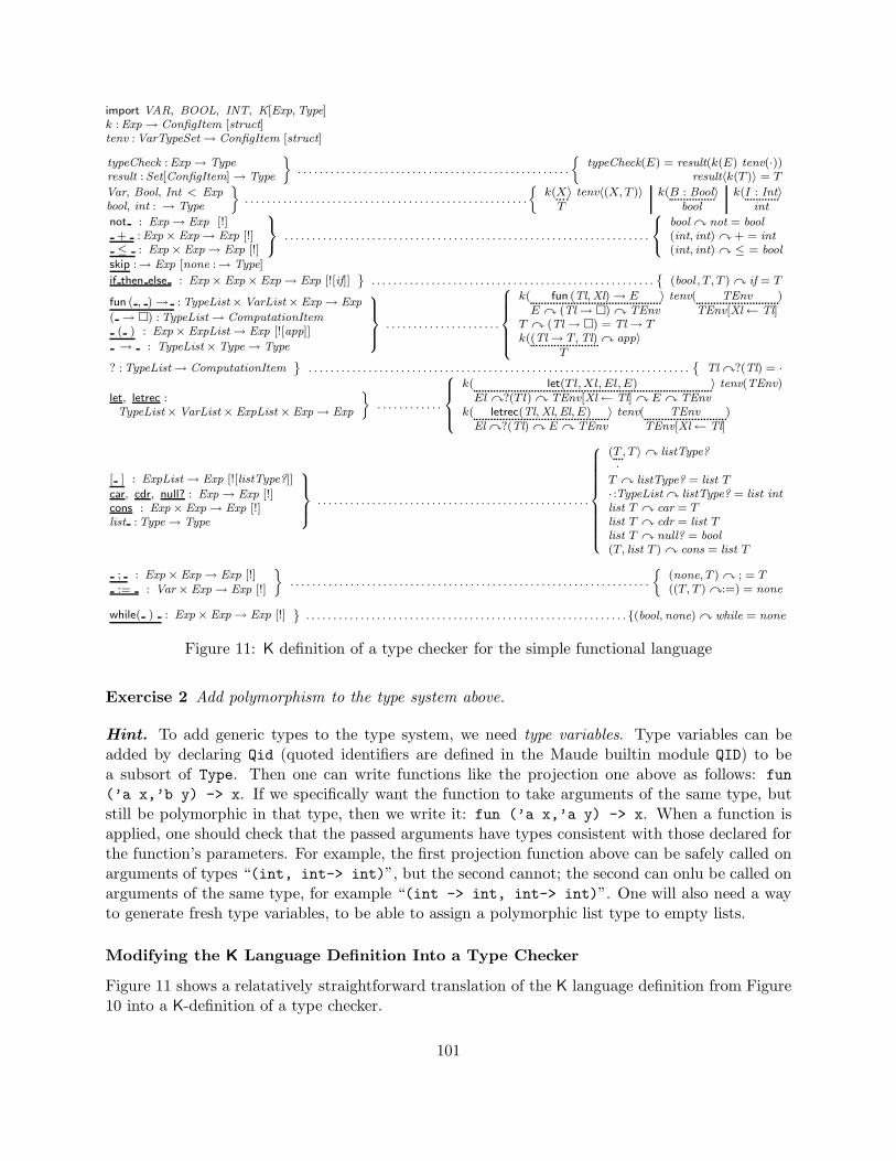
import VAR, BOOL, INT, K[Exp, Type]k :Exp→ ConfigItem [struct]tenv :VarTypeSet→ ConfigItem [struct]

typeCheck :Exp→ Typeresult : Set[ConfigItem]→ Type

ff. . . . . . . . . . . . . . . . . . . . . . . . . . . . . . . . . . . . . . . . . . . . . . . . . .

jtypeCheck(E) = result(k(E) tenv(·))

result〈k(T )〉 = T

Var, Bool, Int < Expbool, int : → Type

ff. . . . . . . . . . . . . . . . . . . . . . . . . . . . . . . . . . . . . . . . . . . . . . . . . . . .

jk(X

T〉 tenv〈(X, T )〉 k(B : Bool

bool〉 k(I : Int

int〉

not : Exp→ Exp [!]+ :Exp× Exp→ Exp [!]≤ : Exp × Exp→ Exp [!]

9=; . . . . . . . . . . . . . . . . . . . . . . . . . . . . . . . . . . . . . . . . . . . . . . . . . . . . . . . . . . . . . . . . . . .

8<:

bool � not = bool(int, int) � + = int(int, int) � ≤ = bool

skip :→ Exp [none :→ Type]

if then else : Exp× Exp× Exp→ Exp [![if]]¯

. . . . . . . . . . . . . . . . . . . . . . . . . . . . . . . . . . . . . . . . . . . . . . . . . . . .˘

(bool , T, T ) � if = T

fun ( , )→ : TypeList× VarList× Exp→ Exp

( → �) : TypeList→ ComputationItem( ) : Exp× ExpList→ Exp [![app]]

→ : TypeList× Type→ Type

9>>=>>; . . . . . . . . . . . . . . . . . . . . .

8>>>><>>>>:

k( fun (Tl,Xl)→ EE � (Tl→ �) � TEnv

〉 tenv( TEnvTEnv[Xl← Tl]

)

T � (Tl→ �) = Tl→ Tk((Tl→ T, Tl)

T� app〉

? :TypeList→ ComputationItem¯

. . . . . . . . . . . . . . . . . . . . . . . . . . . . . . . . . . . . . . . . . . . . . . . . . . . . . . . . . . . . . . . . . . . . . .˘

Tl �?(Tl) = ·

let, letrec :TypeList×VarList× ExpList× Exp→ Exp

ff. . . . . . . . . . . .

8>><>>:

k( let(T l, Xl, El,E)El �?(T l) � TEnv[Xl← Tl] � E � TEnv

〉 tenv(TEnv)

k( letrec(Tl, Xl,El, E)El �?(Tl) � E � TEnv

〉 tenv( TEnvTEnv[Xl← Tl]

)

[ ] : ExpList→ Exp [![listType?]]

car, cdr, null? : Exp→ Exp [!]cons : Exp× Exp→ Exp [!]list :Type→ Type

9>>=>>; . . . . . . . . . . . . . . . . . . . . . . . . . . . . . . . . . . . . . . . . . . . . . . . . . .

8>>>>>>>>><>>>>>>>>>:

(T·, T 〉� listType?

T � listType? = list T· :TypeList � listType? = list intlist T � car = Tlist T � cdr = list Tlist T � null? = bool(T, list T ) � cons = list T

; : Exp× Exp→ Exp [!]:= : Var× Exp→ Exp [!]

ff. . . . . . . . . . . . . . . . . . . . . . . . . . . . . . . . . . . . . . . . . . . . . . . . . . . . . . . . . . . . . . . . . .

j(none, T ) � ; = T((T, T ) �:=) = none

while( ) : Exp× Exp→ Exp [!]¯

. . . . . . . . . . . . . . . . . . . . . . . . . . . . . . . . . . . . . . . . . . . . . . . . . . . . . . . . . . .{(bool, none) � while = none

Figure 11: K definition of a type checker for the simple functional language

Exercise 2 Add polymorphism to the type system above.

Hint. To add generic types to the type system, we need type variables. Type variables can beadded by declaring Qid (quoted identifiers are defined in the Maude builtin module QID) to bea subsort of Type. Then one can write functions like the projection one above as follows: fun(’a x,’b y) -> x. If we specifically want the function to take arguments of the same type, butstill be polymorphic in that type, then we write it: fun (’a x,’a y) -> x. When a function isapplied, one should check that the passed arguments have types consistent with those declared forthe function’s parameters. For example, the first projection function above can be safely called onarguments of types “(int, int-> int)”, but the second cannot; the second can onlu be called onarguments of the same type, for example “(int -> int, int-> int)”. One will also need a wayto generate fresh type variables, to be able to assign a polymorphic list type to empty lists.

Modifying the K Language Definition Into a Type Checker

Figure 11 shows a relatatively straightforward translation of the K language definition from Figure10 into a K-definition of a type checker.

101

Exercise 3 Translate the K-definition of the type checker in Figure 11 into Maude.

102

10.2 Type Inference

Checking that operations are applied on arguments of correct types statically has, as we havealready discussed, two major benefits:

• Allows efficient implementations of programming languages by assuming untyped memorymodels and therefore removing the need for runtime consistency checks, and

• Gives rapid feedback to users, so they can correct errors at early stages.

These advantages are typically considered so major in the programming language community,that the potential drawbacks of static typing, namely

• Limiting the way programs are written by rejecting programs which do not type-check, and

• Adding typing information may be space and time consuming,

are often ignored.The first drawback is usually addressed by rewriting the code in a way that passes the type

checking procedure. For example, programs passing a function as an argument to itself, which donot type check because of the recursive nature of the type of that function, can be replaced byequivalent programs using letrec.

It is, of course, desirable to require the user to provide as little type information as possible aspart of a program. In general, depending on the application and domain of interest, there are quitesubtle trade-offs between the amount of user-provided annotations and the degree of automationof the static analyzer.

In the previous section we discussed a simple static type checker which requires the user toprovide a type for each declared name. Since some names can be functions taking functions asarguments, the amount and shape of these type annotations can be quite heavy. In some cases theymay even exceed the size of the program itself. In this section we address the problem of reducingthe amount of required type information by devising automatic procedures that infer the intendedtypes from how the names are used.

How much type information can be automatically and efficiently inferred depends again upon theparticular domain of interest and its associated type system. In this section we will see an extremefortunate situation, in which all the needed type information can be inferred automatically.

More precisely, we will discuss a classical procedure that infers all the types of all the declarednames in our functional programming language. A similar technique is implemented as part of theML and OCaml languages. By “type”, we here mean the language specific types, that is, those thatwere explicitly provided by users to the static type checker that we discussed.

Type Inference

Programs written in the functional language discussed so far contain all the information that oneneeds in order to infer the intended type of each name. By carefully collecting and using all thisinformation, one can type check programs without the need for the user to provide any auxiliarytype information.

Suppose that one writes the expression x + y as part of a larger expression. Then one can inferfrom here that x and y are both intended to be integers, because the arithmetic operation + isdefined only on integers! Similarly, if

103

if x then y else z

occurs in an expression, then one can deduce, thanks to the typing policy associated to conditionals,that x has type bool and that y and z have the same type. Moreover, from

if x then y else z + t

one can deduce that z and t are both of type integer, implying that y is also integer. Typeinference and type checking work smoothly together, in the sense that one implicitly checks thetypes while inferring information. For example, if

if x then y else z + x

is seen then one knows that there is a typing error because the type of x cannot be both integerand bool.

The type of functions can also be deduced from the way the functions are used. For example,if one uses f(x,y) in some program then one can infer that f takes two arguments. Moreover, iff(x,x) is seen then one can additionally infer that f’s arguments have the same type.

There can be possible that the result type of a function as well as the types of its argumentscan all be inferred from the context, without even analyzing the definition of the function. Forexample, if one writes

f(x,y) + x + let x = y in x

then one first infers that f must return an int because it is used as an argument of + , then thatx is an integer for the same reason, so the type of f’s first argument is int, and finally, because ofthe let which is used in a context of an int, that the type of y is also int. Therefore, the typeof f must be (int,int) -> int. In fact, the types of all the names occurring in the expressionabove were deduced by just analyzing carefully how they are used.

Let us now consider an entire expression which evaluates properly, for example one defining andusing a factorial function:

letrec f(n) = if n eq 0then 1else n * f(n - 1)

in f(5)

How can one automatically infer that this expression is type safe? Since eq takes two ints andreturns a bool, one can deduce that the parameter of the function is int. Further, since the foccurs in the context of an integer and takes an expression which is supposed to be an integer asargument, n - 1, one can deduce that the type of that f is int -> int. Because of the semanticsof letrec, the bound f will have the same type, so the type of the entire expression will be int.

One can infer/check the types differently, obtaining the same result.

Polymorphic Functions

Let us consider again the polymorphic “projection” function which takes two arguments and returnsits first one: fun(x,y) -> x. Without any additional type information, the best one can say aboutthe type of this expression is that it is (t1, t2) -> t1, for some types t1 and t2. This function can benow used in any context in which its result type equals that of its first argument, such as, ((int

104

-> int), int) -> (int -> int). The type of such polymorphic functions should be thought ofas the most general, in the sense of the least constrained, type that one can associate them.

Let us consider several other polymorphic functions. For example, the type of the function fun(x,y) -> x y, which applies its first argument, expected therefore to be a function, to its secondargument, is (t1 -> t2, t1) -> t2.

How can one infer the most general type of an expression then, by just analyzing it syntactically?The process of doing this is called type inference and consists of two steps:

1. Collect information under the form of type parametric constraints by recursively analyzingthe expression;

2. Solve those constraints.

Collecting Type Information

In order to collect type information from an expression, we traverse the expression recursively,assign generic types to certain names and expressions, and then constrain those types. Let usconsider, for example., the expression

fun (x,y) -> if x eq x + 1 then x else y

and let us manually simulate the type information collecting algorithm.We have a function expression. Without additional information, the best we can do is to assume

some generic types for its parameters and then calculate the type of its body. Let tx and ty be thegeneric types of x and y, respectively. If te is the type of function’s body expression, then the typeof the function will be

(tx, ty) -> te.

Let us now calculate the type te while gathering type information as we traverse the body of thefunction.

The body of the function is a conditional, so we can now state a first series of constraints byanalyzing the typing policy of the conditional: its condition is of type bool and its two branchingexpressions must have the same type, which will replace te. Assuming that tb, t1 and t2 are thetypes of its condition and branching expressions, respectively, then we can state the type constrains

tb = bool, andt1 = t2.

We next calculate the types tb, t1 and t2, collecting also the corresponding type information.The types t1 and t2 are easy to calculate because they can be simply extracted from the typeenvironment: tx and ty, respectively (thus, the type equation t1 = t2 above is in fact tx = ty).

To type the condition x eq x + 1, one needs to use the typing policy of eq : takes twoarguments of type int and returns type bool. Thus tb is the type bool, but two new type constraintsare generated, namely

t3 = int, andt4 = int,

105

where t3 and t4 are the types of the two subexpressions of eq . t3 evaluates to tx; in order toevaluate t4 one needs to apply the typing policy of + : takes two int arguments and returns anint. These generate the constraint

tx = int.

Therefore, after “walking” through all the expression and analyzing how names were used, wecollected the following useful typing information:

tx = ty,tx = int, andthe type of the original expression is (tx, ty) -> tx.

After we learn how to solve such type constraint equational systems we will be able to infer fromhere that the expression is correctly typed and its type is (int, int) -> int.

Let us now consider the polymorphic function

fun (x,y) -> (x y) + 1.

After assigning generic types tx and ty to its parameters, while applying the typing policy on+ one can infer that the type of the expression(x y), say t(xy), must be int. Also, the result typeof the function must be int. When calculating t(xy), by applying the typing policy for functionapplication, which says that the type of (E El) for expression E and expression list El is T wheneverthe type of E is Tl -> T and that of El is Tl, one infers the type equational constraint tx = ty ->t(xy). We have accumulated the following type information:

t(xy) = int,tx = ty -> t(xy), andthe type of the function is (tx, ty) -> int.

We will be able to infer from here that the type of the function is (t -> int, t) -> int, so thefunction is polymorphic in t.

The Constraint Collecting Technique

One can collect type constraints in different ways. We will do it by recursively traversing theexpression to type only once, storing a type environment as well as type constrains. If the expressionis

• a name then we return its type from the type environment and collect no auxiliary typeconstraint;

• an integer or a bool constant, then we return its type and collect no constraint;

• an arithmetic operator then we recursively calculate the types of its operand expressionsaccumulating the corresponding constraints, then add the type constraints that their type isint, and then return int;

• a boolean operator then we act like before, but return bool;

106

• a conditional then calculate the types of its three subexpressions accumulating all the typeconstraints, then add two more constraints: one stating that the type of its first subexpressionis bool, and another stating that the types of its other two subexpressions are equal.

• a function then generate a fresh generic type for its parameter, if any, bind it in the typeenvironment accordingly, calculate the type of the body expression in the new environmentaccumulating all the constraints, and then return the corresponding function type;

• a function application then generate a fresh type t, calculate the type of the function ex-pression, say tf , and that of the argument expression list, say tl accumulating all the typeconstraints, and then add the type constraint tf = tl -> t.

• a declaration of names in a let, then calculate the types of the bound expressions, bind themto the corresponding names in the type environment, and then calculate and return the typeof let’s body; there are no additional type constrains to accumulate (besides those in thebound expressions and body);

• a declaration of names in a letrec, then assign some generic types to these names in the typeenvironment, calculate the types of bound expressions and accumulate the constraint(s) thatthese must be equal to the generic types assigned to letrec’s names, and finally calculateand return the type of letrec’s body;

• a list expression, then calculate the types of all the elements in the list accumulating all thecorresponding constraints, and then add the additional constraints that all these types mustbe equal (let T be that type) and finally return the type of the list expression as list T; ifthe list is empty, then T must be a fresh type variable;

• a list operation, such as car, cdr, cons or null?, then calculate the types of the correspond-ing subexpressions accumulating the constraints and then adding new, straightforward typeconstraints; for example, in the case of cons(E,E’), add the constraint that the type of E’must be list T, where T is the type of E;

• an assignment X := E, then calculate the types of X and E, and then add the constraint thatthese two types must be equal.

• a sequential composition E ; E’, then calculate the types of E and E’ accumulating all thetype constraints, then return the type of E’ as the type of the composition;

• a loop while Cond Body, then calculate the types of Cond and Body, add the constraint thatthe type of Cond must be bool, and then return the type none.

Exercise 4 The type inference technique discussed below is based on a divide-and-conquer of themain task: we first collect all the type constraints as equations, and then solve the type constraints.Define a type inferencer that solves the equational type constraints on-the-fly, as they are generated;this would correspoond to doing “online unification”.

107

Defining a Type Constraint Collector

We will use the same programming language and analysis tool equational definitional techniquethat we used to give big-step semantics to FUN and to define its static type checker. Since we willnot need type declarations (all types will be automatically inferred, we can just import the syntaxof the language unchanged from the executable semantics definition.

The TYPE-STATE (module) of our type constraint collector will need to contain three attributes:a type environment, a set of type equations, and a counter needed to generate fresh types.

The constraint collector is defined in the same style as the other tools defined so far, namelyinductively over the structure of the syntax. More precisely, we will define an operation

preType : Exp TypeState -> [Pair]

which calculates the generic type of an expression in a given state, as well as a new state containingall the accumulated constraints. Since experience showed us that it is more convenient to handle listsof expressions in block, we will actually define the preType operator directly on lists of expressions.

We could have defined two distinct operations instead, one returning the type and the other theconstraints (which can be regarded as “side effects”). However, preType will combine both thoseoperators into only one, thus allowing us to design a more compact and more easily understandablespecification.

We call the type returned by preType a pre-type, because in order to calculate the final typewe need to solve the equational constraints. We will first focus on defining preType and then onsolving the type constraints.

In what follows, we only discuss the interesting aspects of the type constraint collector. Moredetails can be found in the file fun-type-inference-semantics.maude on the website, which youare supposed to complete as part of your homework.

Defining Types

Like for the type checker, we introduce a specification defining types. Because of the more complexnature of type inference, and especially because of its ability to infer types in the context ofpolymorphism, we will need more structure on types than before. We declare a subsort TypeVarof the Type and a type variable constructor “op t : Nat -> TypeVar”, which will be used togenerate fresh types as well as to represent polymorphic types:

fmod TYPE is protecting NAT .sorts Type TypeVar TypeList .subsort TypeVar < Type < TypeList .op nil : -> TypeList .op _,_ : TypeList TypeList -> TypeList [assoc id: nil] .ops int bool none : -> Type .op _->_ : TypeList Type -> Type [gather(e E)] .op list_ : Type -> Type [prec 0] .op t : Nat -> TypeVar .

endfm

Defining Type Equations

A type equation is a commutative pair of types. To handle blocks of constraints, we allow equationsof lists of types (defined the usual way in a module TYPE-LIST) and translate them into sets of

108

corresponding equations. The set of equations is kept small by removing the useless ones:

fmod EQUATIONS isprotecting TYPE .sorts Equation Equations .subsorts Equation < Equations .op empty : -> Equations .op _=_ : TypeList TypeList -> Equation [comm] .op _,_ : Equations Equations -> Equations [assoc comm id: empty] .var Eqn : Equation . vars T T’ T1 T1’ : Type . vars Tl Tl’ : TypeList .eq Eqn, Eqn = Eqn .eq (T = T) = empty .eq (T,T1,Tl = T’,T1’,Tl’) = (T = T’), (T1,Tl = T1’,Tl’) .

endfm

Defining the State Infrastructure

The state of the type inferencer will need to contain three attributes: a type environment bindingnames to generic types, a set of equational type constraints, and a counter giving the next “free”type variable. The state can be easily defined by extending the state of the type checker discussedin the previous section with the two additional attributes.

fmod TYPE-STATE isextending TYPE-ENVIRONMENT .extending EQUATIONS .sorts TypeStateAttribute TypeState .subsort TypeStateAttribute < TypeState .op empty : -> TypeState .op __ : TypeState TypeState -> TypeState [assoc comm id: empty] .op tenv : TypeEnv -> TypeStateAttribute .op eqns : Equations -> TypeStateAttribute .op nextType : Nat -> TypeStateAttribute .

endfm

Several standard helping operations are also needed and defined in a module HELPING-OPERATIONS.Only two helping operations are worthwhile discussing, namely:

op freshTypeVar : Nat TypeState -> Pair .eq freshTypeVar(0, S) = {nil,S} .ceq freshTypeVar(s(#), nextType(N) S) = {(t(N),Tl), Sl}if {Tl,Sl} := freshTypeVar(#, nextType(N + 1) S) .

...op _&_ : TypeState Equations -> TypeState .eq (eqns(Eqns) S) & Eqns’ = eqns(Eqns, Eqns’) S .

freshTypeVar takes a natural number # and a state and generates # “fresh” types together withthe new state (containing an updated counter for fresh types). This operation will be intensivelyused in the sequel. S & Eqns collects the the equations in Eqns into the state S.

109

Pre-Typing Generic Expressions

We next define the operation preType taking an expression and a state and returning a pair type-state, where the returned type is a temporary type calculated for the expression; that type will be“evaluated” into a concrete type only after solving the type constraints that are collected in thereturned state.

The preType of integers and names is straightforward, because there is no constraint that needsto be collected:

eq preType(I, S) = {int, S} .eq preType(X, S) = {S[X], S} .

As usual, we prefer to work with lists of expressions. Constraints must be properly accumulatedwhen pre-typing lists of expressions:

ceq preType((E,E’,El), S) = {(T,Tl), Sl}if {T,S’} := preType(E,S)/\ {Tl,Sl} := preType((E’,El),S’) .

Pre-Typing Arithmetic and Boolean Expressions

When we pre-type an arithmetic or boolean operator, there are two things that we should consider,both derived from the typing policy of the language:

1. What are the expected types of its arguments and of its result;

2. How to propagate the type constraints.

...ceq preType(E + E’, S) = {int, S’ & (T,T’ = int,int)}if {(T,T’), S’} := preType((E,E’), S) .

...ceq preType(E leq E’, S) = {bool, S’ & (T,T’ = int,int)}if {(T,T’), S’} := preType((E,E’), S) .

...

Pre-Typing the Conditional

The following definition is self-explanatory: pre-type the condition to Tb and the two branches toT and T’, respectively, and then add the appropriate type constraints:

ceq preType(if BE then E else E’, S) = {T, S’ & (Tb,T = bool,T’)}if {(Tb,T,T’), S’} := preType((BE,E,E’), S) .

Pre-Typing Functions

As usual, we have to consider the two language constructs related to functions, namely functiondeclaration and function invocation. For function declarations, the returned pre-type is the functiontype calculated as follows:

110

ceq preType(fun Xl -> E, S) = {Tl -> Tr, Sr[tenv <- tenv(S)]}if {Tl,Sp} := freshTypeVar(#(Xl),S)/\ {Tr, Sr} := preType(E, Sp[Xl <- Tl]) .

Therefore, a “fresh” type is generated for the function’s parameters, then the body of thefunction is pre-typed in the properly modified state, and then the resulting function type is returned.To be consistent with the semantics of FUN, the returned state forgets the parameter bindings.However, note that the type constraints are not forgotten! They will be needed at the end ofpre-typing.

Function invocations are a bit tricky, because fresh types need to be generated. More precisely,a fresh type is generated for each function invocation, and it is assumed to be the type of the result.Knowing that type, we can generate the appropriate constraints:

ceq preType(F El, S) = {Tr, Sr & (Tf = Tl -> Tr)}if {(Tf,Tl), Sf} := preType((F,El), S)/\ {Tr,Sr} := freshTypeVar(1,Sf) .

It is important to understand the need for the fresh type generated for the result of the function.One may argue that it is not needed, because one can simply pre-type F, which should pre-typeto a function type Tp -> Tr, then E to some Tp’, and then return the type Tr and generate theobvious constraint Tp = Tp’. However, the problem is that E may not pre-type to a function type!

Consider, for example, the expression fun (x,y) -> (x y). When pre-typing (x y), the onlything known about x is that it has some generic type, say t(0). y has also a generic type, sayt(1). Then how about the type of (x y)? By generating a fresh type, say t(2), for the result ofthe function application (x y), we can conclude that the type of x should be t(1) -> t(2), so wecan generate the appropriate type constraint.

Pre-Typing Let

In order to pre-type let, we first pre-type each bound expression and collect all the generated typeconstraints, then we assign fresh generic types to the names to be bound and add new correspondingtype constraints, and then finally pre-type the body of the let.

ceq preType(let(Xl,El,E), S) = {Te, Se[tenv <- tenv(S)]}if {Tel,Sel} := preType(El,S)/\ {Te,Se} := preType(E, Sel[Xl <- Tel]) .

Notice that there are no additional type constraints to be propagated, and that, like for func-tions, the state which is returned after pre-typing let forgets the bindings added to pre-type itsbody, but retains all the generated type constraints as well as the new value of the fresh typecounter!

Pre-Typing Lists

As mentioned earlier, the typing policy of a list is that all its elements have the same type. Toensure this, we need to pre-type all the expressions in a list and to impose the constraints thatall their types are equal. This can be done with one additional operator and a correspondingconditional equation:

111

op preTypeL : ExpList TypeState -> [Pair] .ceq preTypeL(E,El, S) = {T, S’’ & (T = T’)}if {T,S’} := preType(E, S)/\ {T’,S’’} := preTypeL(El, S’) .eq preTypeL(nil,S) = freshTypeVar(1,S) .

The returned type can be any of the types that occurred in the list; we chose the first one.We have seen that the empty list should have a polymorphic type. We can ensure that easily bygenerating a “fresh” type for the pretype of an empty list.

Now a list can be pre-typed as follows:

ceq preType([El], S) = {list T, S’}if {T,S’} := preTypeL(El, S) .

The list operators can be pre-typed in a similar way. For example:

ceq preType(car(E), S) = {T?, S’ & (list T? = T)}if {T?,S?} := freshTypeVar(1,S)/\ {T,S’} := preType(E, S?) .

Solving the Type Constraints

We can pre-type all the other language constructs in a very similar way (this will be part of yourhomework). Thus, the operator preType will take an expression and return a pair {T,S}, where Tis a term of sort Type and eqns(S) contains all the type constraints accumulated by traversing theprogram and applying the typing policy. We refer to terms t(0), t(1), ..., as type variables.

We should understand the result {T,S} of preType(E) as follows:

The (final) type of E will be T in which all the type variables will be substituted by thetypes obtained after solving the system of equations in S. E is not guaranteed a type apriori ! If any conflict is detected while solving the system then we say that the processof typing E failed, and we conclude that the expression is not correctly typed.

If Eqns is a set of type equations, that is, a term of sort Equations, and T is a type potentiallyinvolving type variables, then we let Eqns[T] denote the type obtained after solving Eqns and thensubstituting the type variables accordingly in T.

Once such a magic operation [ ] : Equations Type -> [Type] is defined, we can easily findthe desired type of an expression:

ceq type(E) = eqns(S)[T] if {T,S} := preType(E) .

We next describe a simple equational technique to define the operation [ ] : Equations Type-> [Type].

Exercise 5 Complete the definition of the type inferencer in fun-type-inference-semantics.maude.You need to pre-type the remaining language constructs and then to formalize the technique thatwill be next presented.

112

The Type Inference Procedure by Examples

Example 1Let us consider the following expression:

(fun (x,y) -> x y) (fun z -> 2 * z * z * 3, 3)

After pre-typing (do it, using preType on it), we get the pre-type t(4) and a state containingthe three equations:

int = t(3),t(0) = t(1) -> t(2),(t(0),t(1)) -> t(2) = ((t(3) -> int),int) -> t(4)

How can we solve the system of equations above? We can immediately notice that t(3) = int,so we can just substitute t(3) accordingly in the other equations, obtaining:

t(0) = t(1) -> t(2),(t(0),t(1)) -> t(2) = ((int -> int),int) -> t(4)

Moreover, since t(0) = t(1) -> t(2), by substitution we obtain

((t(1) -> t(2)),t(1)) -> t(2) = ((int -> int),int) -> t(4)

Both types in the equation above are function types, so their source and target domains mustbe equal. This observation allows us to generate two other type equations, namely:

(t(1) -> t(2)),t(1) = (int -> int),intt(2) = t(4).

Now, expanding the first equation into two equations and substituting t(2) by t(4), we get:

t(1) -> t(4) = int -> intt(1) = int

Substituting the second equation we get,

int -> t(4) = int -> int

that is, an equality of function types, which yields the following:

int = intt(4) = int.

The first equation is useless and will be promptly removed by the simplifying rule (T = T) =none in EQUATIONS. The second equation gives the desired type of our expression, int.

Example 2Let us now see an example expression which cannot be typed, e.g.:

let x = fun x -> x in (x x)

After pre-typing, we get the type t(1) constrained by:

113

t(0) -> t(0) = (t(0) -> t(0)) -> t(1)

We can already see that this equation is problematic, but let us just follow the procedure blindlyto see what happens. Since both types in the equation are function types, their source and targettypes must be equal, so we can generate the following two equations:

t(0) = t(0) -> t(0),t(0) = t(1)

The first equation is obviously problematic because of its “recursive” nature, but let us ignoreit and substitute the second into the first, obtaining:

t(1) = t(1) -> t(1).

There is no way to continue. The variable t(1) cannot be assigned a type, so the originalexpression cannot be typed.

Unification

The technique that we used to solve the type equations is called unification. In general the equa-tional unification problem can be stated as follows, where we only consider the mono-sorted case.Our particular unification problem fits this framework, because we can consider that we have onlyone sort, Type.

Let Σ be a signature over only one sort, i.e., a set of operations like in Maude, let X be a finiteset of variables, and let

E = {t1 = t′1, ..., tn = t′n | t1, t′1, ..., tn, t′n ∈ TΣ(X)}

be a finite set of pairs of Σ-terms over variables in X, which from now on we call equations.Notice, however, that these are different from the standard equations in equational logic, which arequantified universally.

A map, or a substitution, θ : X → TΣ(X) is called a unifier of E if and only if θ�(ti) = θ�(t′i)for all 1 ≤ i ≤ n, where θ� : TΣ(X)→ TΣ(X) is the natural extension of θ : X → TΣ(X) to entireterms, by substituting each variable x by its corresponding term, θ(x).

A unifier θ : X → TΣ(X) is more general than ϕ : X → TΣ(X) when ϕ can be obtained fromθ by further substitutions; formally, when there is some other map, say ρ : X → TΣ(X), such thatϕ = θ; ρ�, where the composition of function was written sequentially. Let us consider again ourspecial case signature, that of types, and the equations E :t(0) = t(1) -> t(2),t(0) -> t(1) -> t(2) = (t(3) -> t(3)) -> (t(4) -> t(4)) -> t(5).

Here t(0), ..., t(5) are seen as variables in X.One unifier for these equations, say ϕ, takes t(0) to

(int -> int) -> (int -> int),

t(1), t(2) and t(3) to int -> int, and t(4) to int. Another unifier, say θ, takes t(0) to

(t(4) -> t(4)) -> (t(4) -> t(4)),

114

and t(1), t(2) and t(3) to t(4) -> t(4). Then it is clear that θ is more general than ϕ, becauseϕ = θ; ρ�, where ρ simply takes t(4) to int.

If a set of equations E admits a unifier, they are called unifiable. Note that there can besituations, like the ones we have already seen for our special case of signature of types, when a setof equations is not unifiable.

Finding the Most General Unifier

When a set of equations E is unifiable, its most general unifier, written mgu(E) is one which ismore general than any other unifier of E . Note that typically there are more than one mgu.

We will next discuss a general procedure for finding an mgu for a set of equations E overan arbitrary mono-sorted signature Σ. Since we actually need to apply that mgu to the typecalculated by the preType operation for the expression to type, we will provide a technique thatdirectly calculates E [t] for any term t, which calculates the term after applying the substitutionmgu(E) to t, that is, (mgu(E))�(t).

The technique is in fact quite simple. It can be defined entirely equationally, but in order tomake the desired direction clear we write them as rewriting rules (going from left to right). Itconsists of iteratively applying the following two steps to E [t]:

1. (x = u, E)[t] → subst(x, u, E)[subst(x, u, t)], if x is some variable in X, u is a term in TΣ(X)which does not contain any occurrence of x, and subst(x, u, E) and subst(x, u, t) substituteeach occurrence of x in E and t, respectively, by u;

2. (σ(t1, ..., tk) = σ(t′1, ..., t′k), E)[t] → (t1 = t′1, ..., tk = t′k, E)[t], if σ ∈ Σ is some operation of karguments.

Theorem. When none of the steps above can be applied anymore, we obtain a potentiallymodified final set of equations and a final term, say Ef [tf ]. If Ef is empty then tf is (mgu(E))�(t),so it can be returned as the type of the original expression. If Ef is not empty then E is not unifiable,so the original expression cannot be typed.

Let Polymorphism

Unfortunately, our current polymorphic type inference technique is not as general as it could be.Suppose, for example, that one wants to define a function with the purpose of using it on expressionsof various types, such as an identity function. Since the identity function types to a polymorphictype, t(0) -> t(0) or some similar type, one would naturally want to use it in different contexts.After all, that’s the purpose of polymorphism. Unfortunately, our current type inferencer cannottype the following expression, even though it correctly evaluates to int(1):

let f = fun x -> xin if f true then f 1 else f 2

The reason is that f true will already enforce, via the type constraints, the type of f to betrue -> true; then f 1 and f 2 will enforce the type of f to be int -> int, thus leading to acontradiction. Indeed, our type inferencer will reduce E [t], where E is the set of constraints and tis the pre-type of this expression, to Ef [tf ], where Ef is the equation bool=int and tf is int; sinceEf is not empty, the original expression cannot be typed.

115

The example above may look artificial, because one does not have a need to define an identityfunction. Consider a length function instead, which is, naturally, intended to work on lists of anytype:

fun x -> let c = 0in {

while(not null?(x)){

x := cdr(x) ;c := c + 1

} ;c

}

As expected, our type inferencer will type this expression to a polymorphic type, list t(0)-> int. However, if one uses it on a list of concrete type, then t(0) will be unified with that type,thus preventing one from using the length function on other lists of different types. For example,

let l = fun x -> let c = 0in {

while(not null?(x)){x := cdr(x) ;c := c + 1

} ;c

}in l [5 :: 3 :: 1] + l [true :: false :: true]

will not type, even though it correctly evaluates to int(6).This leads to the following natural question, that a programming language designer wishing a

type system on top of his/her language must address: what should one do when valid programs arerejected by the type system? One unsatisfactory possibility is, of course, to require the programmerswrite their programs differently, so that they will be accepted by the type system. Another, betterpossibility is to improve the type system to accept a larger class of programs.

Since reusing is the main motivation for polymorphism, it would practically make no sense todisallow the use of polymorphic expressions in different contexts. Therefore, programming languagescientists fixed the problem above by introducing the important notion of let-polymorphism.

The idea is to type the let language constructs differently. Currently, we first type all thebinding expressions to some (pre-)types, then we bind those types to the corresponding names intothe type environment, and finally we type the body expression in the new environment. This tech-nique is inherently problematic with respect to reuse, because a (polymorphic) binding expressionis enforced to have two different types if used in two different contexts, which is not possible.

The idea of let-polymorphism is to first substitute all the free occurrences of the bound namesinto the body of the let expression by the corresponding binding expressions, and then to typedirectly the body expression. This way, each use of a bound name will be typed locally, thus solvingour problem.

Exercise 6 Modify our current type inferencer to include let-polymorphism. How about letrec?

116

However, a complexity problem is introduced this way: the size of the code can grow exponen-tially and the binding expressions will be (pre-)typed over and over again, even though each timethey will be typed to “almost” the same type (their types will differ by only the names of the typevariables). There is a partial solution to this problem, too, but that is a more advanced topic thatwill be covered in CS522 next semester.

Type Systems May Reject Correct Programs

While static type checkers/inferencers offer a great help to programmers to catch (trivial) errorsat early stages in their programs and to programming language implementers to generate moreefficient code (by assuming the untyped memory model), they have an inherent drawback: theydisallow correct programs which do not type check. In the previous section we saw a fortunate casewhere a type system could be relatively easily extended (let-polymorphism), to allow polymorphicdefinitions to be used as desired. Unfortunately, due to undecidability reasons, for any given(strong) type system, there will always be programs which can evaluate correctly but which willnot type check.

In our context, for example, consider the following expression/program for calculating the lengthof a list without using letrec or loops:

let t f x = if null?(x) then 0 else 1 + f f cdr(x)in let l x = t t x

in l [4 :: 7 :: 2 :: 1 :: 9]

The idea in the program/expression above is to pass the function as an argument to itself; thisway, it will be available, or “seen”, in its own body, thus simulating the behavior of letrec withoutusing it explicitly. That is how (functional) programmers wrote recursive programs in the earlydays of functional programming, when the importance of static scoping was relatively accepted butno clean support for recursion was available. It, indeed, evaluates to int(5) but does not type.Try it!

One may wrongly thing that the above does not type because our type system does not in-clude let-polymorphism. To see that let-polymorphism is not the problem here, one can apply thesubstitutions by hand and thus eliminate the let constructs entirely:

(fun f x -> if null?(x) then 0 else 1 + f f cdr(x))(fun f x -> if null?(x) then 0 else 1 + f f cdr(x))

[4 :: 7 :: 2 :: 1 :: 9]

The above will again evaluate to int(5), but will not type. The set of constraints is reduced tot(6) = t(6) -> list int -> int, reflecting the fact that there is some expression whose typehas a recursive behavior. Indeed, the type of f (any of them) cannot be inferred due to its recursivebehavior.

In fact, the problematic expression is

fun f x -> if null?(x) then 0 else 1 + f f cdr(x)

which cannot be typed because of the circularity in the type of f. No typed functional languagescan actually type this expression. In ML, for example, the same expression, which in ML syntax is

117

fn (f,x) => if null(x) then 0 else 1 + f f tl(x)

generates an error message of the form:

t.sml:16.36-16.49 Error: operator is not a function [circularity]operator: ’Zin expression:f f

Modifying the K Language Definition Into a Type Inferencer

Figure 12 shows a translation of the K language definition from Figure 10 and/or of the K definitionof the type checker in Figure 11 into a K-definition of a type inferencer.

Exercise 7 Translate the K-definition of the type inferencer in Figure 12 into Maude.

118

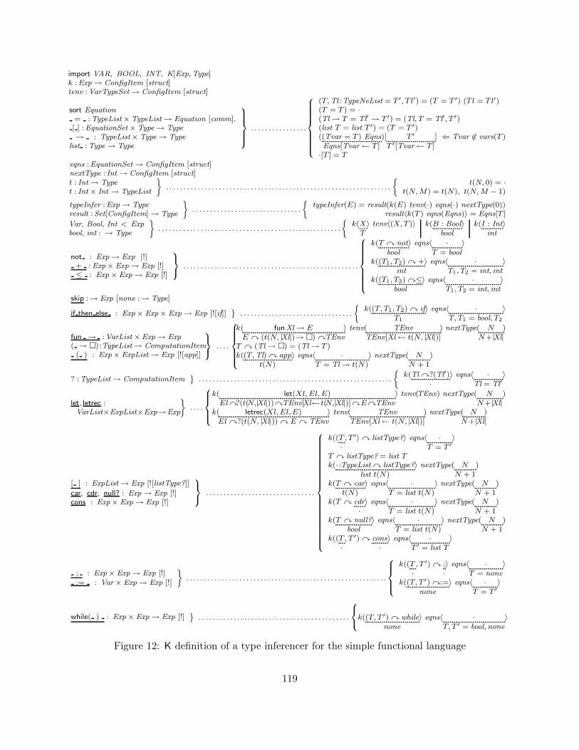
import VAR, BOOL, INT, K[Exp, Type]k :Exp→ ConfigItem [struct]tenv :VarTypeSet→ ConfigItem [struct]

sort Equation= :TypeList×TypeList→ Equation [comm].[ ] :EquationSet × Type→ Type→ : TypeList× Type→ Type

list : Type→ Type

9>>>=>>>;

. . . . . . . . . . . . . . . .

8>>>>>>><>>>>>>>:

(T, Tl :TypeNeList = T ′, T l′) = (T = T ′) (T l = T l′)(T = T ) = ·(Tl→ T = Tl′ → T ′) = (Tl, T = Tl′, T ′)(list T = list T ′) = (T = T ′)((Tvar = T ) EqnsEqns[Tvar← T ]

)[ T ′T ′[Tvar← T ]

] ⇐ Tvar �∈ vars(T )

·[T ] = Teqns :EquationSet→ ConfigItem [struct]nextType : Int→ ConfigItem [struct]t : Int→ Typet : Int× Int→ TypeList

ff. . . . . . . . . . . . . . . . . . . . . . . . . . . . . . . . . . . . . . . . . . . . . . . . . . . . . . . . . . . . . . . .

jt(N, 0) = ·

t(N, M) = t(N), t(N, M − 1)

typeInfer :Exp→ Typeresult : Set[ConfigItem]→ Type

ff. . . . . . . . . . . . . . . . . . . . . . . . . . . . . . .

jtypeInfer(E) = result(k(E) tenv(·) eqns(·) nextType(0))

result〈k(T ) eqns(Eqns)〉 = Eqns[T ]

Var, Bool, Int < Expbool, int : → Type

ff. . . . . . . . . . . . . . . . . . . . . . . . . . . . . . . . . . . . . . . . . . . . . . . . . . . .

jk(X

T〉 tenv〈(X, T )〉 k(B : Bool

bool〉 k(I : Int

int〉

not : Exp→ Exp [!]+ :Exp× Exp→ Exp [!]≤ : Exp × Exp→ Exp [!]

9=; . . . . . . . . . . . . . . . . . . . . . . . . . . . . . . . . . . . . . . . . . . . . . . . . . .

8>>>>>><>>>>>>:

k(T � notbool

〉 eqns〈 ·T = bool

〉

k((T1, T2) � +int

〉 eqns〈 ·T1, T2 = int, int

〉

k((T1, T2) �≤bool

〉 eqns〈 ·T1, T2 = int, int

〉

skip :→ Exp [none :→ Type]

if then else : Exp× Exp× Exp→ Exp [![if]]¯

. . . . . . . . . . . . . . . . . . . . . . . . . . . . . . . .

jk((T, T1, T2) � if

T1

〉 eqns〈 ·T, T1 = bool, T2

〉

fun → :VarList× Exp→ Exp( → �) :TypeList→ ComputationItem( ) : Exp× ExpList→ Exp [![app]]

9=; . . . .

8>>>><>>>>:

k( funXl→ EE � (t(N, |Xl|)→ �) �TEnv

〉 tenv( TEnvTEnv[Xl← t(N, |Xl|)]

) nextType( NN+|Xl|

)

T � (Tl→ �) = (Tl→ T )k((T, Tl) � app

t(N)〉 eqns〈 ·

T = Tl→ t(N)〉 nextType( N

N + 1)

? :TypeList→ ComputationItem¯

. . . . . . . . . . . . . . . . . . . . . . . . . . . . . . . . . . . . . . . . . . . . . . . . . . . . . . .

jk(Tl �?(Tl′)

·〉 eqns〈 ·

Tl = Tl′〉

let, letrec :VarList×ExpList×Exp→Exp

ff. . . .

8>><>>:

k( let(Xl, El, E)El�?(t(N,|Xl|))�TEnv[Xl← t(N,|Xl|)]�E�TEnv

〉 tenv(TEnv) nextType( NN+|Xl|

)

k( letrec(Xl, El,E)El �?(t(N, |Xl|)) � E � TEnv

〉 tenv( TEnvTEnv[Xl← t(N, |Xl|)]

) nextType( NN+|Xl|

)

[ ] : ExpList→ Exp [![listType?]]

car, cdr, null? : Exp→ Exp [!]cons : Exp× Exp→ Exp [!]

9=; . . . . . . . . . . . . . . . . . . . . . . . . . . . . . . .

8>>>>>>>>>>>>>>>>>>>><>>>>>>>>>>>>>>>>>>>>:

k((T·, T ′〉� listType?〉 eqns〈 ·

T = T ′〉

T � listType? = list Tk(· :TypeList � listType?

list t(N)〉 nextType( N

N + 1)

k(T � cart(N)

〉 eqns〈 ·T = list t(N)

〉 nextType( NN + 1

)

k(T � cdr·〉 eqns〈 ·

T = list t(N)〉 nextType( N

N + 1)

k(T � null?bool

〉 eqns〈 ·T = list t(N)

〉 nextType( NN + 1

)

k((T·, T ′) � cons

·〉 eqns〈 ·

T ′ = list T〉

; : Exp× Exp→ Exp [!]:= : Var× Exp→ Exp [!]

ff. . . . . . . . . . . . . . . . . . . . . . . . . . . . . . . . . . . . . . . . . . . . . . . . . . . . . . . . .

8>><>>:

k((T·, T ′) � ;

·〉 eqns〈 ·

T = none〉

k((T, T ′) �:=none

〉 eqns〈 ·T = T ′

〉

while( ) : Exp× Exp→ Exp [!]¯

. . . . . . . . . . . . . . . . . . . . . . . . . . . . . . . . . . . . . . . . . . .

8<:k((T, T ′) � while

none〉 eqns〈 ·

T, T ′ = bool, none〉

Figure 12: K definition of a type inferencer for the simple functional language

119

10.3 Type Preservation and Progress

NEXT-VERSION:

10.4 Concurrency Analysis

NEXT-VERSION:

10.5 Model Checking

NEXT-VERSION:

120

11 On Implementation

NEXT-VERSION:

121

12 Other Applications

...The complete program in K is (the order of rules matters):

import INT, K-BASICk : Comp→ ConfigItem [struct]i, c, d : Int→ ConfigItem [struct]Int < CompItemq : Int→ Intr : Config→ Int

}. . . . . . . . . . . . . . . . . . . . . . . . . . . . . . . . . . . . . . . . . . . . . . . . . . . . .

{q(N) = r(k(0) i(N) c(0) d(1))

r〈k(·) c(I)〉 = I

{ , , } : Int× Comp × Int→ CompItem} . . .

⎧⎪⎪⎪⎪⎪⎪⎪⎪⎪⎪⎪⎪⎨⎪⎪⎪⎪⎪⎪⎪⎪⎪⎪⎪⎪⎩

k(N·〉 i(N) d( D

D − 1)

k( I{I, K, 1}

� K)

k({ , ·, }·〉 i(N) c( J

J + 1) d( N

N − 1)

k({I, ·, }0 � I

〉 d( DD + 1

)

{I, J � K, M} = if |I − J | ∈M 0 then I else {I, K, M + 1}

The Maude-ified version of the K program above is:

fmod M is

protecting INT .

sort Configuration .

op empty : -> Configuration .

op __ : Configuration Configuration -> Configuration [assoc comm id: empty] .

sorts Computation ComputationItem .

subsorts Int ComputationItem < Computation .

op nil : -> Computation .

op _->_ : Computation Computation -> Computation [assoc id: nil] .

op q : Nat -> Nat .

op r : Configuration -> Nat .

vars I J N M D : Int . var K : Computation .

op k : Computation -> Configuration .

ops i c d : Int -> Configuration .

eq q(N) = r(k(0) i(N) c(0) d(1)) .

eq r(k(nil) i(N) c(I) d(D)) = I .

eq k(N -> K) i(N) d(D) = k(K) i(N) d(D - 1) .

eq k(I -> K) i(N) d(M) = k([I + 1, K, 1] -> K) i(N) d(M) [owise] .

eq k([I,nil,M] -> K) i(N) c(J) d(N) = k(K) i(N) c(J + 1) d(N - 1) .

eq k([I,nil,M] -> K) i(N) c(J) d(D) = k(0 -> I -> K) i(N) c(J) d(D + 1) [owise] .

op [_,_,_] : Int Computation Int -> ComputationItem .

eq [I, J -> K, M] = if I == J or I - J == M or J - I == M then I else [I, K, M + 1] fi .

endfm

122

13 Conclusion

An algebraic framework to define programming languages was presented, based on a first-orderrepresentation of continuations and on ACI-matching. The technique was introduced by definingthe language FUN. The language definitions following the discussed methodology are executableby term rewriting, so one can get interpreters for free for the defined languages. Moreover, thesedefinitions can be used to generate, also for free, certain formal analysis tools, such as modelcheckers, for the defined programming languages. As future work, we would like to: (1) implementthe domain-specific language used in this paper; and (2) compile these definitions into efficient coderunning on parallel architectures.

References

[1] G. Agha. Actors. MIT Press, 1986.

[2] J. Bergstra and J. V. Tucker. Equational specs complete term rewriting systems, and com-putable and semicomputable algebras. J. of ACM, 42(6):1194–1230, 1995.

[3] P. Borovansky, H. Cırstea, H. Dubois, C. Kirchner, H. Kirchner, P.-E. Moreau, C. Ringeissen,and M. Vittek. ELAN. User manual – http://www.loria.fr.

[4] C. Braga, E. H. Haeusler, J. Meseguer, and P. D. Mosses. Mapping Modular SOS to RewritingLogic. In M. Leuschel, editor, 12th International Workshop, LOPSTR 2002, Madrid, Spain,volume 2664 of Lecture Notes in Computer Science, pages 262–277, 2002.

[5] M. Clavel, F. J. Duran, S. Eker, P. Lincoln, N. Martı-Oliet, J. Meseguer, and J. F. Que-sada. Maude: Specification and Programming in Rewriting Logic, Mar. 1999. Maude Systemdocumentation at http://maude.csl.sri.com/papers.

[6] R. Diaconescu and K. Futatsugi. CafeOBJ Report. World Scientific, 1998. AMAST Series inComputing, volume 6.

[7] A. Farzan, F. Cheng, J. Meseguer, and G. Rosu. Formal analysis of Java programs in JavaFAN.in Proc. CAV’04, Springer LNCS, 2004.

[8] M. Felleisen and R. Hieb. A Revised Report on the Syntactic Theories of Sequential Controland State. Theoretical Computer Science, 103(2):235–271, 1992.

[9] J. Goguen and G. Malcolm. Alg. Semantics of Imperative Programs. MIT, 1996.

[10] J. Goguen and J. Meseguer. Completeness of many-sorted equational logic. SIGPLAN Notices,16(7):24–37, July 1981.

[11] J. Goguen and J. Meseguer. Order-sorted algebra I: Eq. ded. for multiple inheritance, over-loading, exceptions and partial ops. J. of TCS, 105(2):217–273, 1992.

[12] J. Goguen, J. Thatcher, E. Wagner, and J. Wright. Initial algebra semantics and continuousalgebras. J. of ACM, 24(1):68–95, January 1977.

123

[13] J. Goguen, T. Winkler, J. Meseguer, K. Futatsugi, and J.-P. Jouannaud. Introducing OBJ. InSoft. Eng. with OBJ: alg. spec. in action. Kluwer, 2000.

[14] D. Kapur and P. Narendran. NP-completeness of the set unification and matching problems.In CADE’86, pages 489–495, 1986.

[15] S. Liang, P. Hudak, and M. Jones. Monad transformers and modular interpreters. In POPL’95,pages 333–343. ACM Press, 1995.

[16] N. Martı-Oliet and J. Meseguer. Rewriting logic: roadmap and bibliography. TheoreticalComputer Science, 285:121–154, 2002.

[17] J. Meseguer. Conditional Rewriting Logic as a Unified Model of Concurrency. J. of TCS,96(1):73–155, 1992.

[18] J. Meseguer and G. Rosu. Rewriting logic semantics: From language specifications to formalanalysis tools. In IJCAR’04, pages 1–44. Springer LNAI 3097, 2004.

[19] J. Meseguer and G. Rosu. The rewriting logic semantics project. Technical Report UIUCDCS-R-2005-2639, Deptartment of Computer Science, University of Illinois at Urbana-Champaign,2005.

[20] E. Moggi. An abstract view of programming languages. Technical Report ECS-LFCS-90-113,Edinburgh University, Department of Computer Science, June 1989.

[21] P. D. Mosses. Modular structural operational semantics. J. Log. Algebr. Program., 60–61:195–228, 2004.

[22] G. D. Plotkin. A structural approach to operational semantics. Journal of Logic and AlgebraicProgramming, 60-61:17–139, July-December 2004 2004.

[23] J. C. Reynolds. The Discoveries of Continuations. LISP and Symbolic Computation, 6(3–4):233–247, 1993.

[24] G. Rosu. Programming language classes. Department of Computer Science, University ofIllinois at Urbana-Champaign, http://fsl.cs.uiuc.edu/~grosu/classes/.

[25] T. F. Serbanuta and G. Rosu. Computationally equivalent elimination of conditions - extendedabstract. In Proceedings of Rewriting Techniques and Applications (RTA’06), volume 4098 ofLecture Notes in Computer Science, pages 19–34. Springer, 2006. also appeared as TechnicalReport UIUCDCS-R-2006-2693, February 2006.

[26] C. Strachey and C. P. Wadsworth. Continuations: A Mathematical Semantics for HandlingFull Jumps. Higher-Order and Symb. Computation, 13(1/2):135–152, 2000.

[27] M. G. J. van den Brand, J. Heering, P. Klint, and P. A. Olivier. Compiling lang. defs.:ASF+SDF compiler. ACM Trans. Program. Lang. Syst., 24(4):334–368, 2002.

[28] E. Visser. Program transf. with Stratego/XT: Rules, strategies, tools, and systems. In Domain-Specific Program Generation, pages 216–238, 2003.

124

[29] P. Wadler. The essence of functional programming. pages 1–14, 1992.

[30] M. Walicki and S. Meldal. Algebraic approaches to nondeterminism: An overview. ACMComputing Surveys, 29:30–81, 1997.

125

A A Simple Rewrite Logic Theory in Maude

We here show how the simple rewrite logic theory discussed in Section 3.3 can be formalized inthe Maude system. As one can see, there is an almost zero representational distance in howrewrite theories are specified. Note the use of the operation attributes assoc and comm instead ofthe equations of associativity and commutativity. These attributes are used both by the Maude’sparser (to release the user from providing parentheses for associative operators) and by its rewritingengine: rewrites will be performed modulo operation attributes, enabling specialized algorithms:

mod 01 is

sort S .

op empty : -> S .

op _ _ : S S -> S [assoc comm id: empty] .

op 0 : -> S .

op 1 : -> S .

rl [r1] : 0 => 1 .

rl [r2] : 1 => 0 .

endm

Once a rewrite theory is defined, one can perform different types of analyses. The most obviousone would be to execute it on different terms using the command rewrite, for example:

rewrite 0 1 0 1 0 =>* 1 1 1 1 1 .

The theory above, however, specifies a non-terminating concurrent system. Indeed, the commandabove will never terminate. Therefore, executing the specification above is not interesting. Maudealso provides a search command, which enables a breadth-first search (BFS) state explorationalgorithm on the transition system associated to the term to search from:

search 0 1 0 1 0 =>* 1 1 1 1 1 .

This search command enables the BFS engine to search a path of length zero or more (the “=>*”)from the term 0 1 0 1 0 to the term 1 1 1 1 1. In general, the target term can contain variablesand the search command can take an argument saying how many solutions to search for. In ourcase there is only one solution, found after exploring five additional states. This is Maude’s output:

Solution 1 (state 5)

states: 6 rewrites: 7 in 0ms cpu (0ms real) (~ rewrites/second)

empty substitution

If one wants to see the sequence of states from 0 1 0 1 0 to 1 1 1 1 1, that is, the path to state5 as the above output says, then one can type the command:

show path 5 .

ad get the result:

states: 6 rewrites: 10 in 0ms cpu (0ms real) (~ rewrites/second)

state 0, S: 0 0 0 1 1

===[ rl 0 => 1 [label r1] . ]===>

state 1, S: 0 0 1 1 1

===[ rl 0 => 1 [label r1] . ]===>

state 3, S: 0 1 1 1 1

===[ rl 0 => 1 [label r1] . ]===>

state 5, S: 1 1 1 1 1

126

Finally, if one wants to see all the 6 states explored together with all the transitions in-between,then one can type the command:

show search graph .

and get the result:

state 0, S: 0 0 0 1 1

arc 0 ===> state 1 (rl 0 => 1 [label r1] .)

arc 1 ===> state 2 (rl 1 => 0 [label r2] .)

state 1, S: 0 0 1 1 1

arc 0 ===> state 0 (rl 1 => 0 [label r2] .)

arc 1 ===> state 3 (rl 0 => 1 [label r1] .)

state 2, S: 0 0 0 0 1

arc 0 ===> state 0 (rl 0 => 1 [label r1] .)

arc 1 ===> state 4 (rl 1 => 0 [label r2] .)

state 3, S: 0 1 1 1 1

arc 0 ===> state 1 (rl 1 => 0 [label r2] .)

arc 1 ===> state 5 (rl 0 => 1 [label r1] .)

state 4, S: 0 0 0 0 0

arc 0 ===> state 2 (rl 0 => 1 [label r1] .)

state 5, S: 1 1 1 1 1

arc 0 ===> state 3 (rl 1 => 0 [label r2] .)

As mentioned, the search command allows target terms that may contain variables; this way,the target terms are regarded as patterns. The BFS algorithm will explore the state space of thecorresponding transition system and match each state term against the pattern, reporting all thesuccessful matches by returning the corresponding substitution. For example, one can type thecommand:

search 01 : 0 1 0 0 1 =>* 1 1 1 X:S .

where X:S declares a variable X of sort S on-the-fly (it could have also been declared in the rewritetheory using the syntax “var X : S”). All three solutions will be reported by Maude:

Solution 1 (state 1)

states: 2 rewrites: 1 in 0ms cpu (0ms real) (~ rewrites/second)

X:S --> 0 0

Solution 2 (state 3)

states: 4 rewrites: 3 in 0ms cpu (0ms real) (~ rewrites/second)

X:S --> 0 1

Solution 3 (state 5)

states: 6 rewrites: 7 in 0ms cpu (0ms real) (~ rewrites/second)

X:S --> 1 1

No more solutions.

states: 6 rewrites: 10 in 0ms cpu (0ms real) (~ rewrites/second)

127

The above command investigates the entire state space. Sometimes the state space can beinfinite or very large, and one is not interested in all the solutions of the search anyway. If that isthe case, then one can specify a fixed number of solutions one wants the search command to find;once it succeeds in finding those, the state exploration is terminated. For example, the followingsearch command explores the state space only until it finds two solutions:

search[2] 01 : 0 1 0 0 1 =>* 1 1 1 X:S .

The result shows that only 4 of the total 6 states have been discovered:

Solution 1 (state 1)

states: 2 rewrites: 1 in 0ms cpu (0ms real) (~ rewrites/second)

X:S --> 0 0

Solution 2 (state 3)

states: 4 rewrites: 3 in 0ms cpu (0ms real) (~ rewrites/second)

X:S --> 0 1

Note that, even though the rewrite theory above admits models in which the two rewrite rulescan apply concurrently, for efficiency reasons the search algorithm (as well as the model-checkingone below) explores the state space following an interleaving semantics, i.e., it tries the rules one ata time. This does not imply any unsoundness in reachability (search) analysis because the samestate space is explored anyway.

Let us next formalize in Maude the model-checking example on multi-sets of 0 and 1 discussedin Section 3.3, namely to show that the rewrite theory above does not satisfy the property “it isalways the case that from a state of zeros one can eventually reach a state of ones”. This propertycan be expressed as a linear temporal logic (LTL) formula, namely [](zeros -> <> ones). Touse the model checking capability of Maude, one needs to first import the model checking package(which is only partly builtin; it allows users to add/remove LTL simplification rules) and to definethe atomic predicates. The model checking module comes with a sort State for the states of thetransition system to analyze, with a sort Prop for the atomic propositions on those states, and witha satisfaction operation _|=_ : State Prop -> Bool (defined in the module SATISFACTION). Oneis free to define as many atomic propositions as one wants, but one should make sure that one alsostates when these are true in a given state. For our example, one can do all these as follows:

in MODEL_CHECKER

mod 01-PREDS is

protecting 01 .

including MODEL-CHECKER .

subsort S < State .

var S : S .

op zeros : -> Prop .

eq (1 S) |= zeros = false .

eq (0 S) |= zeros = S |= zeros .

eq empty |= zeros = true .

op ones : -> Prop .

eq (0 S) |= ones = false .

eq (1 S) |= ones = S |= ones .

eq empty |= ones = true .

endm

128

One can now launch the model checking by invoking the operation modelCheck (defined in theMODEL_CHECKER package) on an initial term (whose state space is requested to be model checked)and an LTL formula to be checked against. Below are three invocations of the model checker:

reduce modelCheck(0,[](zeros -> <> ones)) .

reduce modelCheck(0 1,[](zeros -> <> ones)) .

reduce modelCheck(0 1 0 1 0,[](zeros -> <> ones)) .

Interestingly, the first does not violate the property: from the state containing just one 0 there isno way to avoid the state containing just one 1. However, the property is violated, and one possiblecounterexample (not necessarily the smallest one) given, when checked against any multi-set of sizelarger than:

reduce in 01-PREDS : modelCheck(0, [](zeros -> <> ones)) .

rewrites: 18 in 0ms cpu (0ms real) (~ rewrites/second)

result Bool: true

==========================================

reduce in 01-PREDS : modelCheck(0 1, [](zeros -> <> ones)) .

rewrites: 24 in 0ms cpu (0ms real) (~ rewrites/second)

result ModelCheckResult: counterexample({0 1,’r2}, {0 0,’r1} {0 1,’r2})

==========================================

reduce in 01-PREDS : modelCheck(0 1 0 0 1, [](zeros -> <> ones)) .

rewrites: 42 in 0ms cpu (0ms real) (~ rewrites/second)

result ModelCheckResult: counterexample({0 0 0 1 1,’r2} {0 0 0 0 1,’r2} {0 0 0

0 0,’r1} {0 0 0 0 1,’r1} {0 0 0 1 1,’r1}, {0 0 1 1 1,’r1} {0 1 1 1 1,’r2})

This reminds us that, in general, model-checking can find errors in non-deterministic systemsbut it does not prove the correctness of those systems: the fact that a system is model-checkedand shown correct on some inputs does not necessarily imply that the system is correct on all itsinputs.

B Dining Philosophers in Maude

In this appendix we show how the dining philosophers problem discussed in Section 3.3 can bespecified and analyzed in Maude. The following module does nothing but formalizes in Maudethe rewrite logic theory in Section 3.3, replacing the equations of associativity, commutativity andidentity with the corresponding attributes assoc, comm, and id:

mod DINING-PHILOSOPHERS is protecting INT .

--- state infrastructure

sort State .

op empty : -> State .

op __ : State State -> State [assoc comm id: empty] .

op ph : Nat State -> State .

op $ : Nat -> State .

--- number of philosophers + 1

op n : -> Nat .

eq n = 9 .

--- creating the initial state

129

op init : -> State .

eq init = init(n) .

op init : Int -> State .

eq init(-1) = empty .

eq init(N) = ph(N, empty) $(N) init(N - 1) .

vars N X Y : Nat . var Fs : State .

--- acquiring locks: philosophers need to compete on forks

rl ph(N, Fs) $(N) => ph(N, Fs $(N)) .

rl ph(s(N), Fs) $(N) => ph(s(N), Fs $(N)) .

crl ph(0, Fs) $(N) => ph(0, Fs $(n)) if N = n .

--- no competition involved in releasing locks

eq ph(N, $(X) $(Y)) = ph(N, empty) $(X) $(Y) .

endm

To find all the states in which no rules can be applied anymore, or in other words to find all thestates which are normal forms, one needs to use the special symbol “=>!” in the search command:

search init =>! S:State .

The above will return the two deadlock solutions for 10 philosophers in about 2.7 seconds on a2.5GHz/3.5GB Linux machine, while for 14 philosophers (change “n = 9” to “n = 13” in the mod-ule above) in about 400 seconds. In our experiments, Maude crashed when tried on 15 philosopherson the machine above.

C Defining Lists and Sets in Maude

fmod SORT is

sort Sort .

ops a b c : -> Sort .

endfm

fmod SORT-LIST is protecting SORT .

sorts SortList SortNeList .

subsorts Sort < SortNeList < SortList .

op nil : -> SortList .

op _,_ : SortList SortList -> SortList [assoc id: nil] .

op _,_ : SortNeList SortNeList -> SortNeList [ditto] .

endfm

parse a,b,b,c,a,b,c .

parse a .

parse nil .

parse nil,a,nil .

reduce nil,a,nil .

fmod SORT-SET is protecting SORT .

sorts SortSet SortNeSet .

subsorts Sort < SortNeSet < SortSet .

op empty : -> SortSet .

op _ _ : SortSet SortSet -> SortSet [assoc id: empty] .

130

op _ _ : SortNeSet SortNeSet -> SortNeSet [ditto] .

endfm

parse a b b c a b c .

parse a .

parse empty .

parse empty a empty .

reduce empty a empty .

D Definition of Sequential λK in Maude

In this appendix we show an instance of the K-technique presented in the paper, in the contextof the Maude language. The Maude code below is a translation of the K-definition of sequentialλK in Figure 2. Appendix E shows a similar instance, but for the concurrent extension of λK inFigure 4. Appendixes F and G show the more complex Maude instances of the FUN language. Allthe Maude language definitions in Appendixes D, E, F and G, have been hand-crafted by TraianFlorin Serbanuta (to whom I warmly thank for his continuous help and interest in this project) ina few hours, by following a mechanical K-to-Maude translation procedure that he is also currentlyimplementing.

At this moment, in our Maude-ified K language definitions we collapse the sorts Exp andContinuation; we assume that programs are syntactically well-formed, in particular that one doesnot explicitly use K continuations in programs (some external parser or static checker can be usedfor this purpose as well). One should not find it surprising that expressions and continuationsare collapsed in our semantics; in our framework, continuations are nothing but computationallyequivalent variants of expressions that are structurally more suitable for defining the semantics ofother operators.

fmod SYNTAX is

including INT .

including QID .

--- Var

sort Var .

subsort Qid < Var .

ops a b c d e f g h i j k l m n o p q r t u v x y z : -> Var [format (g o)] .

sort Exp .

subsort Var < Exp .

op #_ : Int -> Exp [prec 30 format (b r o)] .

ops _+_ _-_ : Exp Exp -> Exp [prec 33 gather (E e) format (d b o d)] .

ops _*_ _/_ : Exp Exp -> Exp [prec 32 gather (E e) format (d b o d)] .

ops true false : -> Exp [format (r o)] .

ops _<=_ _>=_ _==_ : Exp Exp -> Exp [prec 37 format (d b o d)] .

op _and_ : Exp Exp -> Exp [prec 55 format (d b o d)] .

op _or_ : Exp Exp -> Exp [prec 57 format (d b o d)] .

op not_ : Exp -> Exp [prec 53 format (b o d)] .

sort VarList ExpList .

op _,_ : VarList VarList -> VarList [assoc id: .] .

op . : -> VarList .

131

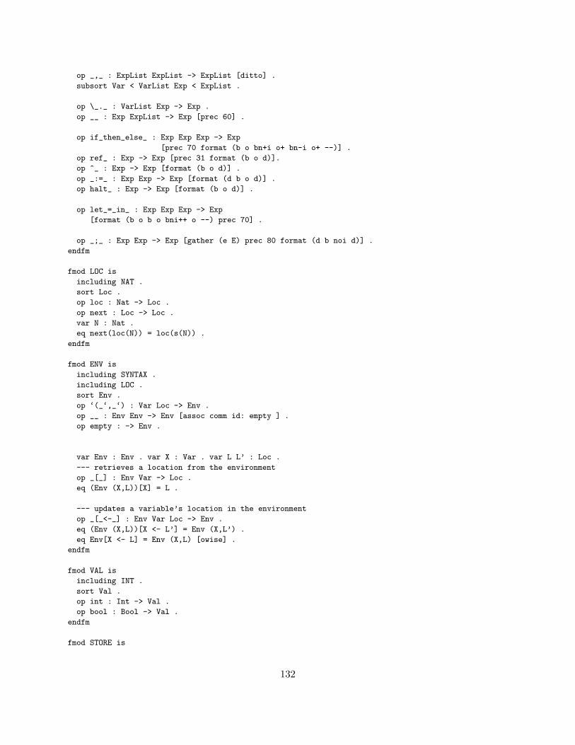
op _,_ : ExpList ExpList -> ExpList [ditto] .

subsort Var < VarList Exp < ExpList .

op \_._ : VarList Exp -> Exp .

op __ : Exp ExpList -> Exp [prec 60] .

op if_then_else_ : Exp Exp Exp -> Exp

[prec 70 format (b o bn+i o+ bn-i o+ --)] .

op ref_ : Exp -> Exp [prec 31 format (b o d)].

op ^_ : Exp -> Exp [format (b o d)] .

op _:=_ : Exp Exp -> Exp [format (d b o d)] .

op halt_ : Exp -> Exp [format (b o d)] .

op let_=_in_ : Exp Exp Exp -> Exp

[format (b o b o bni++ o --) prec 70] .

op _;_ : Exp Exp -> Exp [gather (e E) prec 80 format (d b noi d)] .

endfm

fmod LOC is

including NAT .

sort Loc .

op loc : Nat -> Loc .

op next : Loc -> Loc .

var N : Nat .

eq next(loc(N)) = loc(s(N)) .

endfm

fmod ENV is

including SYNTAX .

including LOC .

sort Env .

op ‘(_‘,_‘) : Var Loc -> Env .

op __ : Env Env -> Env [assoc comm id: empty ] .

op empty : -> Env .

var Env : Env . var X : Var . var L L’ : Loc .

--- retrieves a location from the environment

op _[_] : Env Var -> Loc .

eq (Env (X,L))[X] = L .

--- updates a variable’s location in the environment

op _[_<-_] : Env Var Loc -> Env .

eq (Env (X,L))[X <- L’] = Env (X,L’) .

eq Env[X <- L] = Env (X,L) [owise] .

endfm

fmod VAL is

including INT .

sort Val .

op int : Int -> Val .

op bool : Bool -> Val .

endfm

fmod STORE is

132

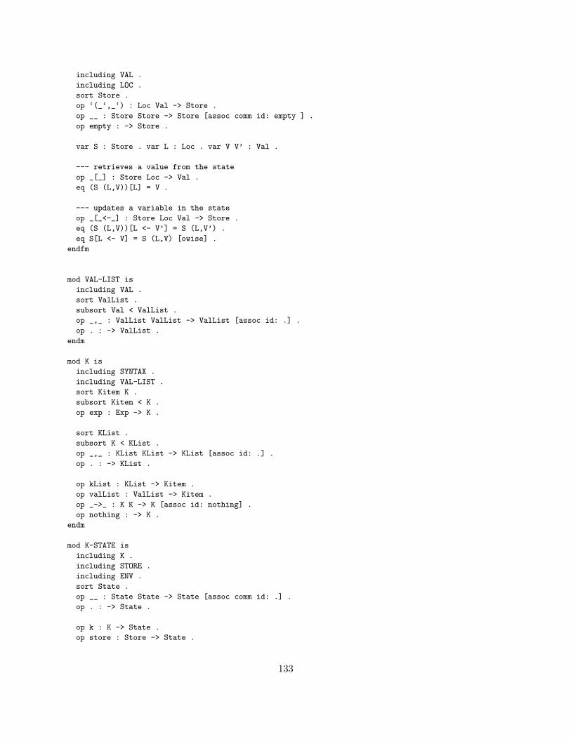
including VAL .

including LOC .

sort Store .

op ‘(_‘,_‘) : Loc Val -> Store .

op __ : Store Store -> Store [assoc comm id: empty ] .

op empty : -> Store .

var S : Store . var L : Loc . var V V’ : Val .

--- retrieves a value from the state

op _[_] : Store Loc -> Val .

eq (S (L,V))[L] = V .

--- updates a variable in the state

op _[_<-_] : Store Loc Val -> Store .

eq (S (L,V))[L <- V’] = S (L,V’) .

eq S[L <- V] = S (L,V) [owise] .

endfm

mod VAL-LIST is

including VAL .

sort ValList .

subsort Val < ValList .

op _,_ : ValList ValList -> ValList [assoc id: .] .

op . : -> ValList .

endm

mod K is

including SYNTAX .

including VAL-LIST .

sort Kitem K .

subsort Kitem < K .

op exp : Exp -> K .

sort KList .

subsort K < KList .

op _,_ : KList KList -> KList [assoc id: .] .

op . : -> KList .

op kList : KList -> Kitem .

op valList : ValList -> Kitem .

op _->_ : K K -> K [assoc id: nothing] .

op nothing : -> K .

endm

mod K-STATE is

including K .

including STORE .

including ENV .

sort State .

op __ : State State -> State [assoc comm id: .] .

op . : -> State .

op k : K -> State .

op store : Store -> State .

133

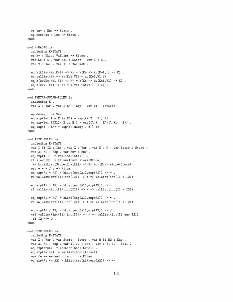
op env : Env -> State .

op nextLoc : Loc -> State .

endm

mod K-BASIC is

including K-STATE .

op kv : KList ValList -> Kitem .

var Ke : K . var Kel : KList . var K : K .

var V : Val . var Vl : ValList .

eq k(kList(Ke,Kel) -> K) = k(Ke -> kv(Kel,.) -> K) .

eq valList(V) -> kv(Kel,Vl) = kv(Kel,Vl,V) .

eq k(kv(Ke,Kel,Vl) -> K) = k(Ke -> kv(Kel,Vl) -> K) .

eq k(kv(.,Vl) -> K) = k(valList(Vl) -> K) .

endm

mod SYNTAX-SUGAR-RULES is

including K .

var X : Var . var E E’ : Exp . var Xl : VarList .

op dummy : -> Var .

eq exp(let X = E in E’) = exp((\ X . E’) E) .

eq exp(let X(Xl)= E in E’) = exp((\ X . E’)(\ Xl . E)) .

eq exp(E ; E’) = exp((\ dummy . E’) E) .

endm

mod AEXP-RULES is

including K-STATE .

var I I1 I2 : Int . var X : Var . var K : K . var Store : Store .

var A1 A2 : Exp . var Env : Env .

eq exp(# I) = valList(int(I)) .

rl k(exp(X) -> K) env(Env) store(Store)

=> k(valList(Store[Env[X]]) -> K) env(Env) store(Store) .

ops + - * / : -> Kitem .

eq exp(A1 + A2) = kList(exp(A1),exp(A2)) -> + .

rl valList(int(I1),int(I2)) -> + => valList(int(I1 + I2)) .

eq exp(A1 - A2) = kList(exp(A1),exp(A2)) -> - .

rl valList(int(I1),int(I2)) -> - => valList(int(I1 - I2)) .

eq exp(A1 * A2) = kList(exp(A1),exp(A2)) -> * .

rl valList(int(I1),int(I2)) -> * => valList(int(I1 * I2)) .

eq exp(A1 / A2) = kList(exp(A1),exp(A2)) -> / .

crl valList(int(I1),int(I2)) -> / => valList(int(I1 quo I2))

if I2 =/= 0 .

endm

mod BEXP-RULES is

including K-STATE .

var X : Var . var Store : Store . var B B1 B2 : Exp .

var A1 A2 : Exp . var I1 I2 : Int . var T T1 T2 : Bool .

eq exp(true) = valList(bool(true)) .

eq exp(false) = valList(bool(false)) .

ops <= >= == and or not : -> Kitem .

eq exp(A1 <= A2) = kList(exp(A1),exp(A2)) -> <= .

134

rl valList(int(I1),int(I2)) -> <= => valList(bool(I1 <= I2)) .

eq exp(A1 >= A2) = kList(exp(A1),exp(A2)) -> >= .

rl valList(int(I1),int(I2)) -> >= => valList(bool(I1 >= I2)) .

eq exp(A1 == A2) = kList(exp(A1),exp(A2)) -> == .

rl valList(int(I1),int(I2)) -> == => valList(bool(I1 == I2)) .

eq exp(B1 and B2) = kList(exp(B1),exp(B2)) -> and .

rl valList(bool(T1),bool(T2)) -> and => valList(bool(T1 and T2)) .

eq exp(B1 or B2) = kList(exp(B1),exp(B2)) -> or .

rl valList(bool(T1),bool(T2)) -> or => valList(bool(T1 or T2)) .

eq exp(not B) = exp(B) -> not .

rl valList(bool(T)) -> not => valList(bool(not T)) .

endm

mod FUNCTION-RULES is

including K-STATE .

op closure : VarList K Env -> Val .

var Xl : VarList . var E : Exp . var El : ExpList . var X : Var .

var Env Env’ : Env . var V : Val . var Vl : ValList . var K K’ : K .

var Store : Store . var L : Loc .

eq k(exp(\ Xl . E) -> K) env(Env)

= k(valList(closure(Xl,exp(E),Env)) -> K) env(Env) .

op bind : VarList -> Kitem .

eq k(valList(Vl,V) -> bind(Xl,X) -> K)

env(Env) store(Store) nextLoc(L)

= k(valList(Vl) -> bind(Xl) -> K)

env(Env[X <- L]) store(Store (L,V)) nextLoc(next(L)) .

eq k(valList(.) -> bind(.) -> K) = k(K) .

op app : -> Kitem .

eq exp(E El) = kList(exp(E),expList(El)) -> app .

op expList : ExpList -> KList .

eq expList(E,El) = exp(E),expList(El) .

eq expList(.) = . .

rl k(valList(closure(Xl,K,Env),Vl) -> app -> K’) env(Env’)

=> k(valList(Vl) -> bind(Xl) -> K -> restore(Env’) -> K’) env(Env) .

op restore : Env -> Kitem .

eq k(restore(Env) -> K) env(Env’) = k(K) env(Env) .

endm

mod IMPERATIVE-RULES is

including K-STATE .

op loc : Loc -> Val .

ops ref ^ := halt : -> Kitem .

op if : K K -> Kitem .

var E E1 E2 E’ : Exp . var K K’ K1 K2 : K . var L : Loc .

var V V’ : Val . var Store : Store .

eq exp(if E then E1 else E2) = exp(E) -> if(exp(E1),exp(E2)) .

rl k(valList(bool(true)) -> if(K1,K2) -> K) => k(K1 -> K) .

rl k(valList(bool(false)) -> if(K1,K2) -> K) => k(K2 -> K) .

eq exp(ref E) = exp(E) -> ref .

rl k(valList(V) -> ref -> K) nextLoc(L) store(Store)

=> k(valList(loc(L)) -> K) nextLoc(next(L)) store(Store (L,V)) .

135

eq exp(^ E) = exp(E) -> ^ .

rl k(valList(loc(L)) -> ^ -> K) store(Store (L,V))

=> k(valList(V) -> K) store(Store (L,V)) .

eq exp(E := E’) = kList(exp(E),exp(E’)) -> := .

rl k(valList(loc(L),V) -> := -> K) store(Store (L,V’))

=> k(valList(V) -> K) store(Store (L,V)) .

eq exp(halt E) = exp(E) -> halt .

rl k(valList(V) -> halt -> K) => k(valList(V)) .

endm

mod K-SEMANTICS is

including K-BASIC .

including SYNTAX-SUGAR-RULES .

including AEXP-RULES .

including BEXP-RULES .

including FUNCTION-RULES .

including IMPERATIVE-RULES .

op <_> : Exp -> [Val] .

op result : State -> [Val] .

var P : Exp . var V : Val . var Store : Store . var Env : Env .

var L : Loc .

eq < P >

= result(k(exp(P)) env(empty) store(empty) nextLoc(loc(0))) .

eq result(k(valList(V)) env(Env) store(Store) nextLoc(L))

= V .

endm

rew < let r = ref # 100 in

let g m,h = if m >= # 2

then r := ^ r * m ;

h m - # 1,h

else halt ^ r

in g # 100 - # 1,g > .

***> should compute 100!

quit

E Definition of Concurrent λK in Maude

In this appendix we show the Maude-ified version of the concurrent λK language, whose K-definitionis shown in Figure 4. Note that there is much repetition between the subsequent definition and theone of sequential λK in Appendix D, but yet, we cannot just import sequential λK and define theadditional features on top of it, as we did in K. That is because rewriting logic semantics is not asmodular as K is in what regards changes of the state structure. Once we have an implementationof K together with translations into Maude and/or other rewrite engines, definitions like those inAppendix D and in this appendix, as well as those in Appendixes F and G, can all be generatedautomatically from the corresponding modular K definitions.

fmod SYNTAX is

including INT .

136

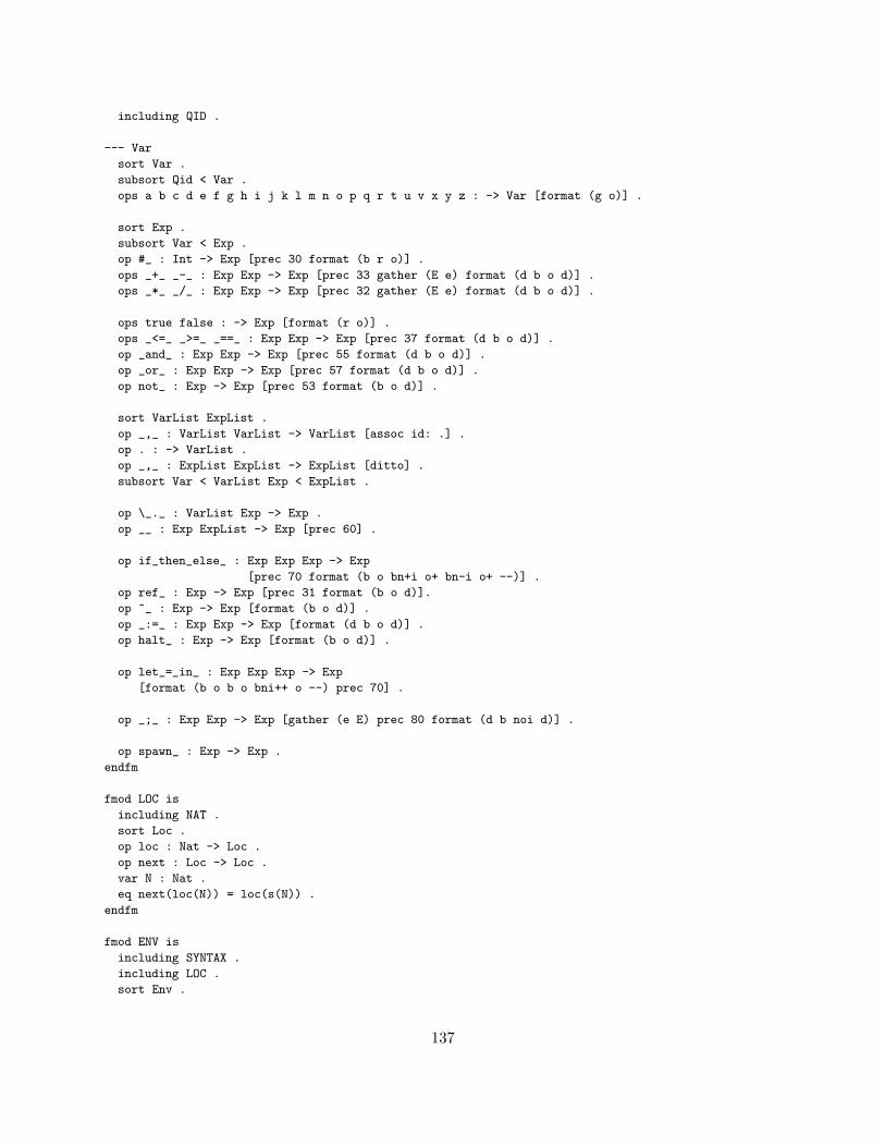
including QID .

--- Var

sort Var .

subsort Qid < Var .

ops a b c d e f g h i j k l m n o p q r t u v x y z : -> Var [format (g o)] .

sort Exp .

subsort Var < Exp .

op #_ : Int -> Exp [prec 30 format (b r o)] .

ops _+_ _-_ : Exp Exp -> Exp [prec 33 gather (E e) format (d b o d)] .

ops _*_ _/_ : Exp Exp -> Exp [prec 32 gather (E e) format (d b o d)] .

ops true false : -> Exp [format (r o)] .

ops _<=_ _>=_ _==_ : Exp Exp -> Exp [prec 37 format (d b o d)] .

op _and_ : Exp Exp -> Exp [prec 55 format (d b o d)] .

op _or_ : Exp Exp -> Exp [prec 57 format (d b o d)] .

op not_ : Exp -> Exp [prec 53 format (b o d)] .

sort VarList ExpList .

op _,_ : VarList VarList -> VarList [assoc id: .] .

op . : -> VarList .

op _,_ : ExpList ExpList -> ExpList [ditto] .

subsort Var < VarList Exp < ExpList .

op \_._ : VarList Exp -> Exp .

op __ : Exp ExpList -> Exp [prec 60] .

op if_then_else_ : Exp Exp Exp -> Exp

[prec 70 format (b o bn+i o+ bn-i o+ --)] .

op ref_ : Exp -> Exp [prec 31 format (b o d)].

op ^_ : Exp -> Exp [format (b o d)] .

op _:=_ : Exp Exp -> Exp [format (d b o d)] .

op halt_ : Exp -> Exp [format (b o d)] .

op let_=_in_ : Exp Exp Exp -> Exp

[format (b o b o bni++ o --) prec 70] .

op _;_ : Exp Exp -> Exp [gather (e E) prec 80 format (d b noi d)] .

op spawn_ : Exp -> Exp .

endfm

fmod LOC is

including NAT .

sort Loc .

op loc : Nat -> Loc .

op next : Loc -> Loc .

var N : Nat .

eq next(loc(N)) = loc(s(N)) .

endfm

fmod ENV is

including SYNTAX .

including LOC .

sort Env .

137

op ‘(_‘,_‘) : Var Loc -> Env .

op __ : Env Env -> Env [assoc comm id: empty ] .

op empty : -> Env .

var Env : Env . var X : Var . var L L’ : Loc .

--- retrieves a location from the environment

op _[_] : Env Var -> Loc .

eq (Env (X,L))[X] = L .

--- updates a variable’s location in the environment

op _[_<-_] : Env Var Loc -> Env .

eq (Env (X,L))[X <- L’] = Env (X,L’) .

eq Env[X <- L] = Env (X,L) [owise] .

endfm

fmod VAL is

including INT .

sort Val .

op int : Int -> Val .

op bool : Bool -> Val .

endfm

fmod STORE is

including VAL .

including LOC .

sort Store .

op ‘(_‘,_‘) : Loc Val -> Store .

op __ : Store Store -> Store [assoc comm id: empty ] .

op empty : -> Store .

var S : Store . var L : Loc . var V V’ : Val .

--- retrieves a value from the state

op _[_] : Store Loc -> Val .

eq (S (L,V))[L] = V .

--- updates a variable in the state

op _[_<-_] : Store Loc Val -> Store .

eq (S (L,V))[L <- V’] = S (L,V’) .

eq S[L <- V] = S (L,V) [owise] .

endfm

mod VAL-LIST is

including VAL .

sort ValList .

subsort Val < ValList .

op _,_ : ValList ValList -> ValList [assoc id: .] .

op . : -> ValList .

endm

mod K is

including SYNTAX .

including VAL-LIST .

sort Kitem K .

138

subsort Kitem < K .

op exp : Exp -> K .

sort KList .

subsort K < KList .

op _,_ : KList KList -> KList [assoc id: .] .

op . : -> KList .

op kList : KList -> Kitem .

op valList : ValList -> Kitem .

op _->_ : K K -> K [assoc id: nothing] .

op nothing : -> K .

endm

mod K-THREAD-STATE is

including K .

including ENV .

sort ThreadState .

op __ : ThreadState ThreadState -> ThreadState [assoc comm id: .] .

op . : -> ThreadState .

op k : K -> ThreadState .

op env : Env -> ThreadState .

endm

mod K-STATE is

including STORE .

including K-THREAD-STATE .

sort State .

op __ : State State -> State [assoc comm id: .] .

op . : -> State .

op thread : ThreadState -> State .

op store : Store -> State .

op nextLoc : Loc -> State .

endm

mod K-BASIC is

including K-STATE .

op kv : KList ValList -> Kitem .

var Ke : K . var Kel : KList . var K : K .

var V : Val . var Vl : ValList .

eq k(kList(Ke,Kel) -> K) = k(Ke -> kv(Kel,.) -> K) .

eq valList(V) -> kv(Kel,Vl) = kv(Kel,Vl,V) .

eq k(kv(Ke,Kel,Vl) -> K) = k(Ke -> kv(Kel,Vl) -> K) .

eq k(kv(.,Vl) -> K) = k(valList(Vl) -> K) .

endm

mod SYNTAX-SUGAR-RULES is

including K .

var X : Var . var E E’ : Exp . var Xl : VarList .

op dummy : -> Var .

eq exp(let X = E in E’) = exp((\ X . E’) E) .

eq exp(let X(Xl)= E in E’) = exp((\ X . E’)(\ Xl . E)) .

eq exp(E ; E’) = exp((\ dummy . E’) E) .

139

endm

mod AEXP-RULES is

including K-STATE .

var I I1 I2 : Int . var X : Var . var K : K . var Store : Store .

var A1 A2 : Exp . var Env : Env .

eq exp(# I) = valList(int(I)) .

rl thread(k(exp(X) -> K) env(Env)) store(Store)

=> thread(k(valList(Store[Env[X]]) -> K) env(Env)) store(Store) .

ops + - * / : -> Kitem .

eq exp(A1 + A2) = kList(exp(A1),exp(A2)) -> + .

rl valList(int(I1),int(I2)) -> + => valList(int(I1 + I2)) .

eq exp(A1 - A2) = kList(exp(A1),exp(A2)) -> - .

rl valList(int(I1),int(I2)) -> - => valList(int(I1 - I2)) .

eq exp(A1 * A2) = kList(exp(A1),exp(A2)) -> * .

rl valList(int(I1),int(I2)) -> * => valList(int(I1 * I2)) .

eq exp(A1 / A2) = kList(exp(A1),exp(A2)) -> / .

crl valList(int(I1),int(I2)) -> / => valList(int(I1 quo I2))

if I2 =/= 0 .

endm

mod BEXP-RULES is

including K-STATE .

var B B1 B2 : Exp .

var A1 A2 : Exp . var I1 I2 : Int . var T T1 T2 : Bool .

eq exp(true) = valList(bool(true)) .

eq exp(false) = valList(bool(false)) .

ops <= >= == and or not : -> Kitem .

eq exp(A1 <= A2) = kList(exp(A1),exp(A2)) -> <= .

rl valList(int(I1),int(I2)) -> <= => valList(bool(I1 <= I2)) .

eq exp(A1 >= A2) = kList(exp(A1),exp(A2)) -> >= .

rl valList(int(I1),int(I2)) -> >= => valList(bool(I1 >= I2)) .

eq exp(A1 == A2) = kList(exp(A1),exp(A2)) -> == .

rl valList(int(I1),int(I2)) -> == => valList(bool(I1 == I2)) .

eq exp(B1 and B2) = kList(exp(B1),exp(B2)) -> and .

rl valList(bool(T1),bool(T2)) -> and => valList(bool(T1 and T2)) .

eq exp(B1 or B2) = kList(exp(B1),exp(B2)) -> or .

rl valList(bool(T1),bool(T2)) -> or => valList(bool(T1 or T2)) .

eq exp(not B) = exp(B) -> not .

rl valList(bool(T)) -> not => valList(bool(not T)) .

endm

mod FUNCTION-RULES is

including K-STATE .

op closure : VarList K Env -> Val .

var Xl : VarList . var E : Exp . var El : ExpList . var X : Var .

var Env Env’ : Env . var V : Val . var Vl : ValList . var K K’ : K .

var Store : Store . var L : Loc .

140

eq k(exp(\ Xl . E) -> K) env(Env)

= k(valList(closure(Xl,exp(E),Env)) -> K) env(Env) .

op bind : VarList -> Kitem .

eq thread(k(valList(Vl,V) -> bind(Xl,X) -> K) env(Env))

store(Store) nextLoc(L)

= thread(k(valList(Vl) -> bind(Xl) -> K) env(Env[X <- L]))

store(Store (L,V)) nextLoc(next(L)) .

eq k(valList(.) -> bind(.) -> K) = k(K) .

op app : -> Kitem .

eq exp(E El) = kList(exp(E),expList(El)) -> app .

op expList : ExpList -> KList .

eq expList(E,El) = exp(E),expList(El) .

eq expList(.) = . .

rl k(valList(closure(Xl,K,Env),Vl) -> app -> K’) env(Env’)

=> k(valList(Vl) -> bind(Xl) -> K -> restore(Env’) -> K’) env(Env) .

op restore : Env -> Kitem .

eq k(restore(Env) -> K) env(Env’) = k(K) env(Env) .

endm

mod IMPERATIVE-RULES is

including K-STATE .

op loc : Loc -> Val .

ops ref ^ := halt : -> Kitem .

op if : K K -> Kitem .

var E E1 E2 E’ : Exp . var K K’ K1 K2 : K . var L : Loc .

var V V’ : Val . var Store : Store . var TS : ThreadState .

eq exp(if E then E1 else E2) = exp(E) -> if(exp(E1),exp(E2)) .

rl k(valList(bool(true)) -> if(K1,K2) -> K) => k(K1 -> K) .

rl k(valList(bool(false)) -> if(K1,K2) -> K) => k(K2 -> K) .

eq exp(ref E) = exp(E) -> ref .

rl thread(k(valList(V) -> ref -> K) TS)

nextLoc(L) store(Store)

=> thread(k(valList(loc(L)) -> K) TS)

nextLoc(next(L)) store(Store (L,V)) .

eq exp(^ E) = exp(E) -> ^ .

rl thread(k(valList(loc(L)) -> ^ -> K) TS) store(Store (L,V))

=> thread(k(valList(V) -> K) TS) store(Store (L,V)) .

eq exp(E := E’) = kList(exp(E),exp(E’)) -> := .

rl thread(k(valList(loc(L),V) -> := -> K) TS) store(Store (L,V’))

=> thread(k(valList(V) -> K) TS) store(Store (L,V)) .

eq exp(halt E) = exp(E) -> halt .

rl k(valList(V) -> halt -> K) => k(valList(V)) .

endm

mod SPAWN-RULES is

including K-STATE .

op die : -> Kitem .

var E : Exp . var K : K . var Env : Env . var V : Val .

var TS : ThreadState .

rl thread(k(exp(spawn E) -> K) env(Env))

=> thread(k(valList(int(0)) -> K) env(Env))

thread(k(exp(E) -> die) env(Env)) .

rl thread(k(valList(V) -> die) TS) => . .

141

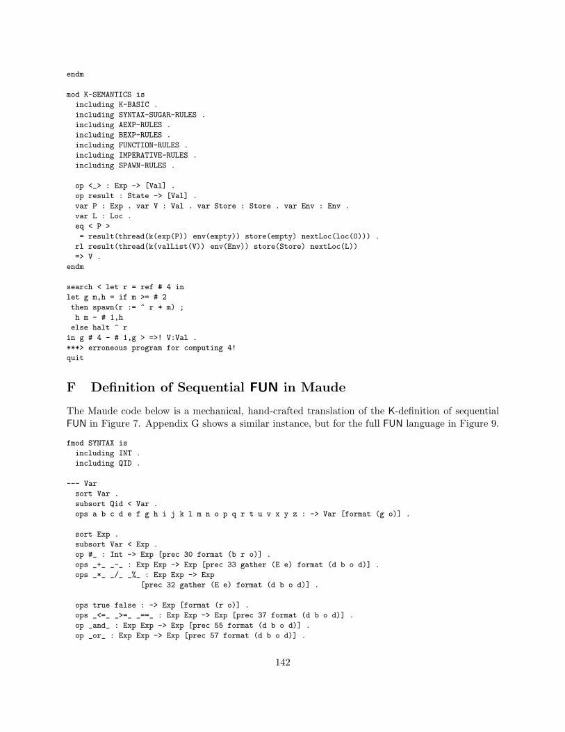
endm

mod K-SEMANTICS is

including K-BASIC .

including SYNTAX-SUGAR-RULES .

including AEXP-RULES .

including BEXP-RULES .

including FUNCTION-RULES .

including IMPERATIVE-RULES .

including SPAWN-RULES .

op <_> : Exp -> [Val] .

op result : State -> [Val] .

var P : Exp . var V : Val . var Store : Store . var Env : Env .

var L : Loc .

eq < P >

= result(thread(k(exp(P)) env(empty)) store(empty) nextLoc(loc(0))) .

rl result(thread(k(valList(V)) env(Env)) store(Store) nextLoc(L))

=> V .

endm

search < let r = ref # 4 in

let g m,h = if m >= # 2

then spawn(r := ^ r * m) ;

h m - # 1,h

else halt ^ r

in g # 4 - # 1,g > =>! V:Val .

***> erroneous program for computing 4!

quit

F Definition of Sequential FUN in Maude

The Maude code below is a mechanical, hand-crafted translation of the K-definition of sequentialFUN in Figure 7. Appendix G shows a similar instance, but for the full FUN language in Figure 9.

fmod SYNTAX is

including INT .

including QID .

--- Var

sort Var .

subsort Qid < Var .

ops a b c d e f g h i j k l m n o p q r t u v x y z : -> Var [format (g o)] .

sort Exp .

subsort Var < Exp .

op #_ : Int -> Exp [prec 30 format (b r o)] .

ops _+_ _-_ : Exp Exp -> Exp [prec 33 gather (E e) format (d b o d)] .

ops _*_ _/_ _%_ : Exp Exp -> Exp

[prec 32 gather (E e) format (d b o d)] .

ops true false : -> Exp [format (r o)] .

ops _<=_ _>=_ _==_ : Exp Exp -> Exp [prec 37 format (d b o d)] .

op _and_ : Exp Exp -> Exp [prec 55 format (d b o d)] .

op _or_ : Exp Exp -> Exp [prec 57 format (d b o d)] .

142

op not_ : Exp -> Exp [prec 53 format (b o d)] .

op skip : -> Exp [format (b o)] .

op if_then_ : Exp Exp -> Exp

[prec 70 format (b o bn+i o+ --)] .

op if_then_else_ : Exp Exp Exp -> Exp

[prec 70 format (b o bn+i o+ bn-i o+ --)] .

sort VarList ExpList .

op _,_ : VarList VarList -> VarList [assoc id: .] .

op . : -> VarList .

op _,_ : ExpList ExpList -> ExpList [ditto] .

subsort Var < VarList Exp < ExpList .

op fun_->_ : VarList Exp -> Exp [format (b o b no++i n--)] .

op _‘(_‘) : Exp ExpList -> Exp [prec 60 format(d b o b o)] .

op return : Exp -> Exp [format (b o)] .

ops let letrec : VarList ExpList Exp -> Exp [format (b o)] .

op _;_ : Exp Exp -> Exp [gather (e E) prec 80 format (d b noi d)] .

op _:=_ : Var Exp -> Exp [format (d b o d)] .

op ‘[_‘] : ExpList -> Exp [format (b o b o)] .

ops car cdr null? : Exp -> Exp [format (b o)] .

op cons : Exp Exp -> Exp [format (b o)] .

op read‘(‘) : -> Exp [format (b d d o)] .

op print : Exp -> Exp [format (b o)] .

op try_catch‘(_‘)_ : Exp Var Exp -> Exp [format (b o b d o b o d)] .

op throw : Exp -> Exp [format (b o)] .

op while‘(_‘)_ : Exp Exp -> Exp [format (b d o b no++i --)] .

op for‘(_;_;_‘)_ : Exp Exp Exp Exp -> Exp

[format (b d o b o b o b no++i --)] .

op break : -> Exp [format (b o)] .

op continue : -> Exp [format (b o)] .

endfm

fmod LOC is

including NAT .

sort Loc .

op loc : Nat -> Loc .

op next : Loc -> Loc .

var N : Nat .

eq next(loc(N)) = loc(s(N)) .

endfm

fmod ENV is

including SYNTAX .

including LOC .

sort Env .

op ‘(_‘,_‘) : Var Loc -> Env .

op __ : Env Env -> Env [assoc comm id: empty ] .

143

op empty : -> Env .

var Env : Env . var X : Var . var L L’ : Loc .

--- retrieves a location from the environment

op _[_] : Env Var -> Loc .

eq (Env (X,L))[X] = L .

--- updates a variable’s location in the environment

op _[_<-_] : Env Var Loc -> Env .

eq (Env (X,L))[X <- L’] = Env (X,L’) .

eq Env[X <- L] = Env (X,L) [owise] .

endfm

fmod VAL is

including INT .

sort Val .

op int : Int -> Val .

op bool : Bool -> Val .

op unit : -> Val .

endfm

fmod STORE is

including VAL .

including LOC .

sort Store .

op ‘(_‘,_‘) : Loc Val -> Store .

op __ : Store Store -> Store [assoc comm id: empty ] .

op empty : -> Store .

var S : Store . var L : Loc . var V V’ : Val .

--- retrieves a value from the state

op _[_] : Store Loc -> Val .

eq (S (L,V))[L] = V .

--- updates a variable in the state

op _[_<-_] : Store Loc Val -> Store .

eq (S (L,V))[L <- V’] = S (L,V’) .

eq S[L <- V] = S (L,V) [owise] .

endfm

mod VAL-LIST is

including VAL .

sort ValList .

subsort Val < ValList .

op _,_ : ValList ValList -> ValList [assoc id: .] .

op . : -> ValList .

endm

mod INT-LIST is

including INT .

sort IntList .

subsort Int < IntList .

op _,_ : IntList IntList -> IntList [assoc id: .] .

op . : -> IntList .

144

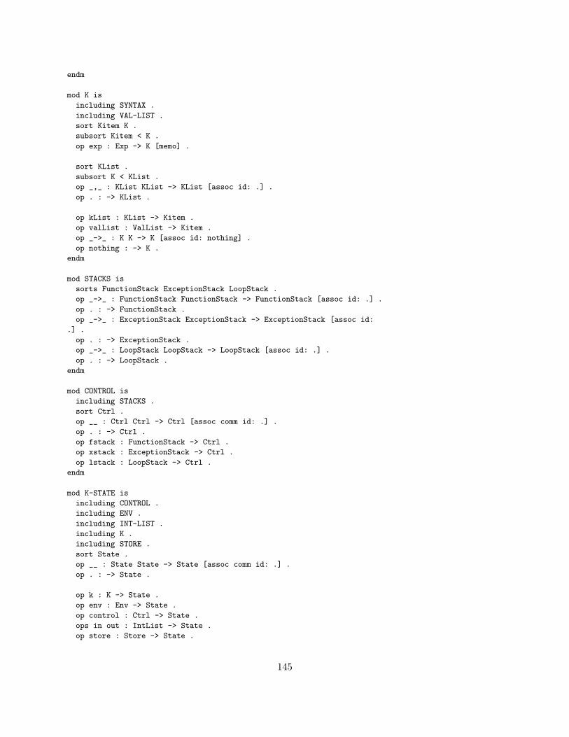
endm

mod K is

including SYNTAX .

including VAL-LIST .

sort Kitem K .

subsort Kitem < K .

op exp : Exp -> K [memo] .

sort KList .

subsort K < KList .

op _,_ : KList KList -> KList [assoc id: .] .

op . : -> KList .

op kList : KList -> Kitem .

op valList : ValList -> Kitem .

op _->_ : K K -> K [assoc id: nothing] .

op nothing : -> K .

endm

mod STACKS is

sorts FunctionStack ExceptionStack LoopStack .

op _->_ : FunctionStack FunctionStack -> FunctionStack [assoc id: .] .

op . : -> FunctionStack .

op _->_ : ExceptionStack ExceptionStack -> ExceptionStack [assoc id:

.] .

op . : -> ExceptionStack .

op _->_ : LoopStack LoopStack -> LoopStack [assoc id: .] .

op . : -> LoopStack .

endm

mod CONTROL is

including STACKS .

sort Ctrl .

op __ : Ctrl Ctrl -> Ctrl [assoc comm id: .] .

op . : -> Ctrl .

op fstack : FunctionStack -> Ctrl .

op xstack : ExceptionStack -> Ctrl .

op lstack : LoopStack -> Ctrl .

endm

mod K-STATE is

including CONTROL .

including ENV .

including INT-LIST .

including K .

including STORE .

sort State .

op __ : State State -> State [assoc comm id: .] .

op . : -> State .

op k : K -> State .

op env : Env -> State .

op control : Ctrl -> State .

ops in out : IntList -> State .

op store : Store -> State .

145

op nextLoc : Loc -> State .

endm

mod K-BASIC is

including K-STATE .

op kv : KList ValList -> Kitem .

var Ke : K . var Kel : KList . var K : K .

var V V’ : Val . var Vl : ValList .

var X : Var . var Xl : VarList . var Env Env’ : Env . var L : Loc .

var E : Exp . var El : ExpList . var Store : Store .

eq k(kList(Ke,Kel) -> K) = k(Ke -> kv(Kel,.) -> K) .

eq valList(V) -> kv(Kel,Vl) = kv(Kel,Vl,V) .

eq k(kv(Ke,Kel,Vl) -> K) = k(Ke -> kv(Kel,Vl) -> K) .

eq k(kv(.,Vl) -> K) = k(valList(Vl) -> K) .

op bind : VarList -> Kitem .

eq k(valList(Vl,V) -> bind(Xl,X) -> K)

env(Env) store(Store) nextLoc(L)

= k(valList(Vl) -> bind(Xl) -> K)

env(Env[X <- L]) store(Store (L,V)) nextLoc(next(L)) .

eq k(valList(.) -> bind(.) -> K) = k(K) .

eq k(bind(Xl,X) -> K)

env(Env) nextLoc(L)

= k(bind(Xl) -> K)

env(Env[X <- L]) nextLoc(next(L)) .

eq k(bind(.) -> K) = k(K) .

op write : VarList -> Kitem .

eq k(valList(Vl,V) -> write(Xl,X) -> K)

env(Env (X,L)) store(Store)

= k(valList(Vl) -> write(Xl) -> K)

env(Env (X,L)) store(Store[L <- V]) .

eq k(valList(.) -> write(.) -> K) = k(K) .

op expList : ExpList -> KList .

eq expList(E,El) = exp(E),expList(El) .

eq expList(.) = . .

op restore : Env -> Kitem .

eq k(valList(V) -> restore(Env) -> K) env(Env’)

= k(valList(V) -> K) env(Env) .

endm

mod AEXP-RULES is

including K-STATE .

var I I1 I2 : Int . var X : Var . var K : K . var Store : Store .

var A1 A2 : Exp . var Env : Env .

eq exp(# I) = valList(int(I)) .

rl k(exp(X) -> K) env(Env) store(Store)

=> k(valList(Store[Env[X]]) -> K) env(Env) store(Store) .

ops + - * / % : -> Kitem .

eq exp(A1 + A2) = kList(exp(A1),exp(A2)) -> + .

rl valList(int(I1),int(I2)) -> + => valList(int(I1 + I2)) .

eq exp(A1 - A2) = kList(exp(A1),exp(A2)) -> - .

146

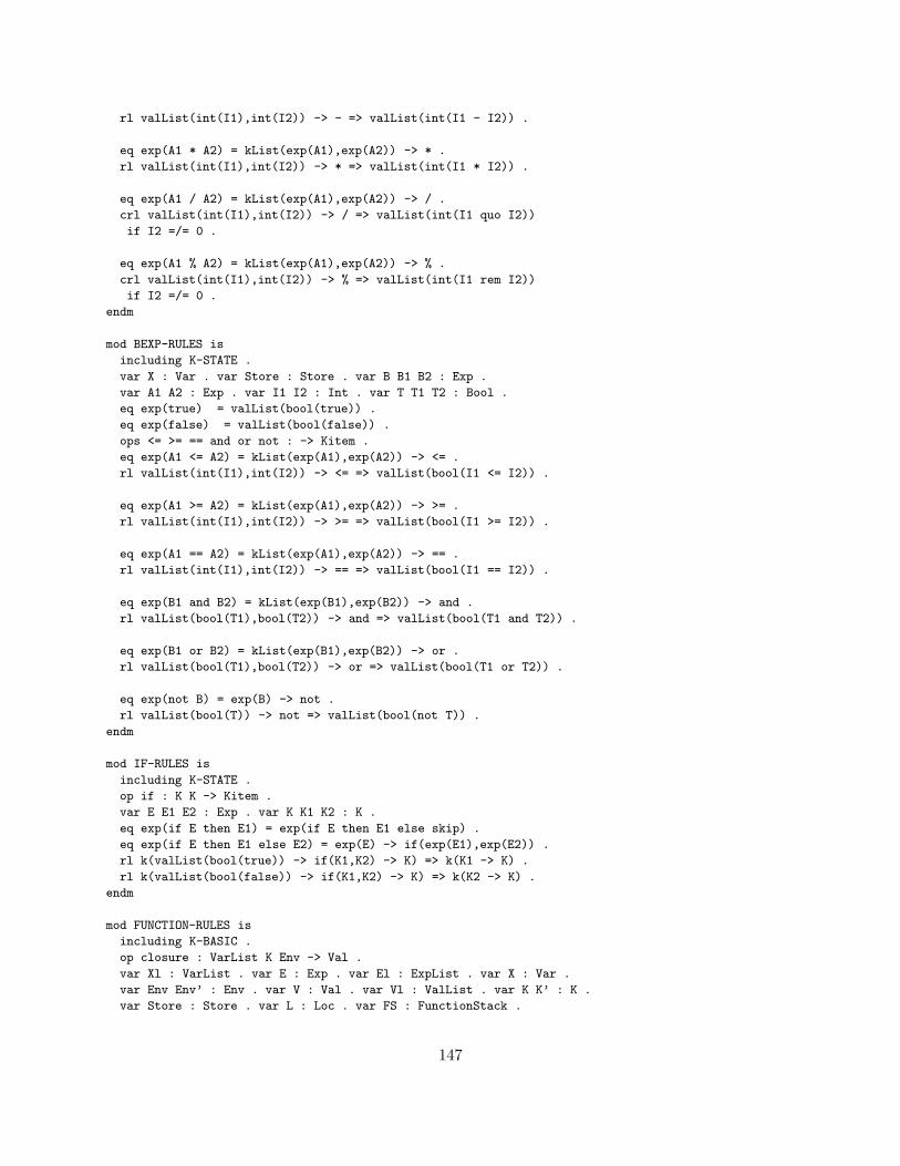
rl valList(int(I1),int(I2)) -> - => valList(int(I1 - I2)) .

eq exp(A1 * A2) = kList(exp(A1),exp(A2)) -> * .

rl valList(int(I1),int(I2)) -> * => valList(int(I1 * I2)) .

eq exp(A1 / A2) = kList(exp(A1),exp(A2)) -> / .

crl valList(int(I1),int(I2)) -> / => valList(int(I1 quo I2))

if I2 =/= 0 .

eq exp(A1 % A2) = kList(exp(A1),exp(A2)) -> % .

crl valList(int(I1),int(I2)) -> % => valList(int(I1 rem I2))

if I2 =/= 0 .

endm

mod BEXP-RULES is

including K-STATE .

var X : Var . var Store : Store . var B B1 B2 : Exp .

var A1 A2 : Exp . var I1 I2 : Int . var T T1 T2 : Bool .

eq exp(true) = valList(bool(true)) .

eq exp(false) = valList(bool(false)) .

ops <= >= == and or not : -> Kitem .

eq exp(A1 <= A2) = kList(exp(A1),exp(A2)) -> <= .

rl valList(int(I1),int(I2)) -> <= => valList(bool(I1 <= I2)) .

eq exp(A1 >= A2) = kList(exp(A1),exp(A2)) -> >= .

rl valList(int(I1),int(I2)) -> >= => valList(bool(I1 >= I2)) .

eq exp(A1 == A2) = kList(exp(A1),exp(A2)) -> == .

rl valList(int(I1),int(I2)) -> == => valList(bool(I1 == I2)) .

eq exp(B1 and B2) = kList(exp(B1),exp(B2)) -> and .

rl valList(bool(T1),bool(T2)) -> and => valList(bool(T1 and T2)) .

eq exp(B1 or B2) = kList(exp(B1),exp(B2)) -> or .

rl valList(bool(T1),bool(T2)) -> or => valList(bool(T1 or T2)) .

eq exp(not B) = exp(B) -> not .

rl valList(bool(T)) -> not => valList(bool(not T)) .

endm

mod IF-RULES is

including K-STATE .

op if : K K -> Kitem .

var E E1 E2 : Exp . var K K1 K2 : K .

eq exp(if E then E1) = exp(if E then E1 else skip) .

eq exp(if E then E1 else E2) = exp(E) -> if(exp(E1),exp(E2)) .

rl k(valList(bool(true)) -> if(K1,K2) -> K) => k(K1 -> K) .

rl k(valList(bool(false)) -> if(K1,K2) -> K) => k(K2 -> K) .

endm

mod FUNCTION-RULES is

including K-BASIC .

op closure : VarList K Env -> Val .

var Xl : VarList . var E : Exp . var El : ExpList . var X : Var .

var Env Env’ : Env . var V : Val . var Vl : ValList . var K K’ : K .

var Store : Store . var L : Loc . var FS : FunctionStack .

147

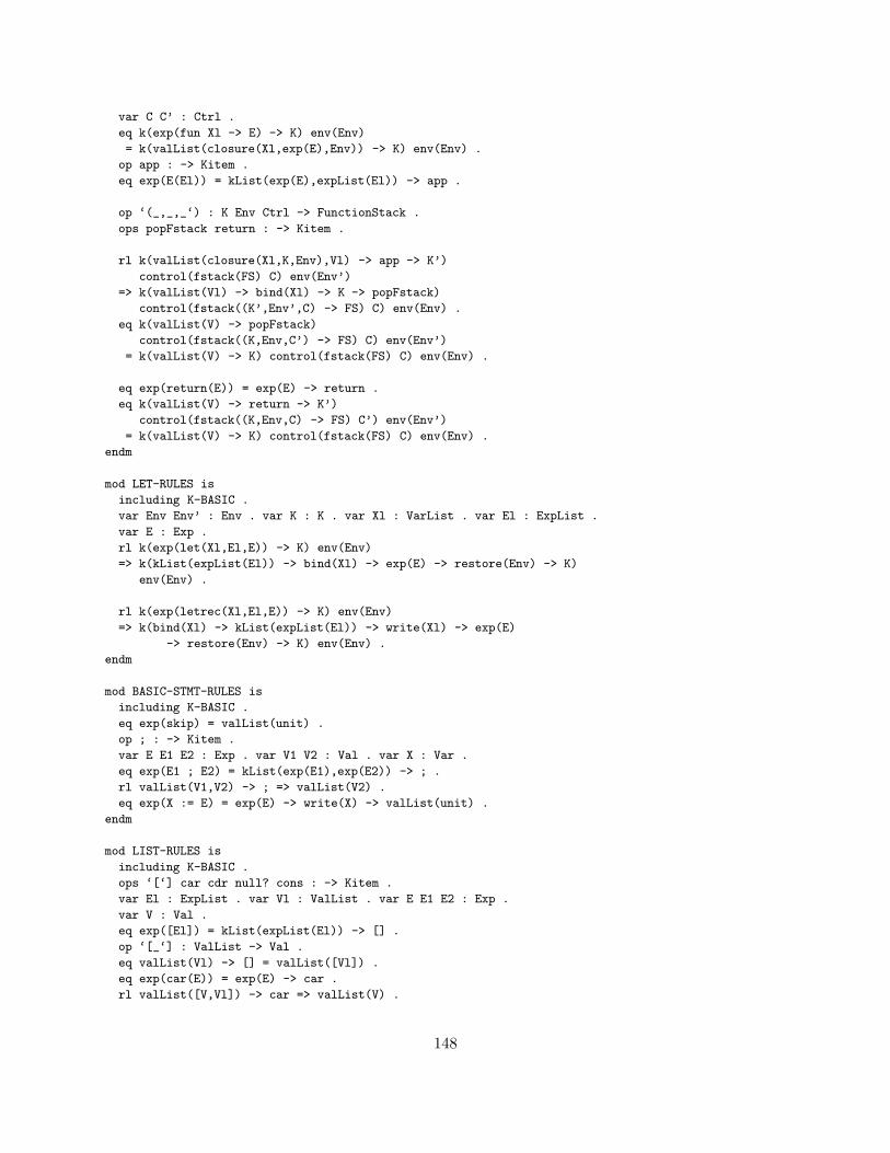
var C C’ : Ctrl .

eq k(exp(fun Xl -> E) -> K) env(Env)

= k(valList(closure(Xl,exp(E),Env)) -> K) env(Env) .

op app : -> Kitem .

eq exp(E(El)) = kList(exp(E),expList(El)) -> app .

op ‘(_,_,_‘) : K Env Ctrl -> FunctionStack .

ops popFstack return : -> Kitem .

rl k(valList(closure(Xl,K,Env),Vl) -> app -> K’)

control(fstack(FS) C) env(Env’)

=> k(valList(Vl) -> bind(Xl) -> K -> popFstack)

control(fstack((K’,Env’,C) -> FS) C) env(Env) .

eq k(valList(V) -> popFstack)

control(fstack((K,Env,C’) -> FS) C) env(Env’)

= k(valList(V) -> K) control(fstack(FS) C) env(Env) .

eq exp(return(E)) = exp(E) -> return .

eq k(valList(V) -> return -> K’)

control(fstack((K,Env,C) -> FS) C’) env(Env’)

= k(valList(V) -> K) control(fstack(FS) C) env(Env) .

endm

mod LET-RULES is

including K-BASIC .

var Env Env’ : Env . var K : K . var Xl : VarList . var El : ExpList .

var E : Exp .

rl k(exp(let(Xl,El,E)) -> K) env(Env)

=> k(kList(expList(El)) -> bind(Xl) -> exp(E) -> restore(Env) -> K)

env(Env) .

rl k(exp(letrec(Xl,El,E)) -> K) env(Env)

=> k(bind(Xl) -> kList(expList(El)) -> write(Xl) -> exp(E)

-> restore(Env) -> K) env(Env) .

endm

mod BASIC-STMT-RULES is

including K-BASIC .

eq exp(skip) = valList(unit) .

op ; : -> Kitem .

var E E1 E2 : Exp . var V1 V2 : Val . var X : Var .

eq exp(E1 ; E2) = kList(exp(E1),exp(E2)) -> ; .

rl valList(V1,V2) -> ; => valList(V2) .

eq exp(X := E) = exp(E) -> write(X) -> valList(unit) .

endm

mod LIST-RULES is

including K-BASIC .

ops ‘[‘] car cdr null? cons : -> Kitem .

var El : ExpList . var Vl : ValList . var E E1 E2 : Exp .

var V : Val .

eq exp([El]) = kList(expList(El)) -> [] .

op ‘[_‘] : ValList -> Val .

eq valList(Vl) -> [] = valList([Vl]) .

eq exp(car(E)) = exp(E) -> car .

rl valList([V,Vl]) -> car => valList(V) .

148

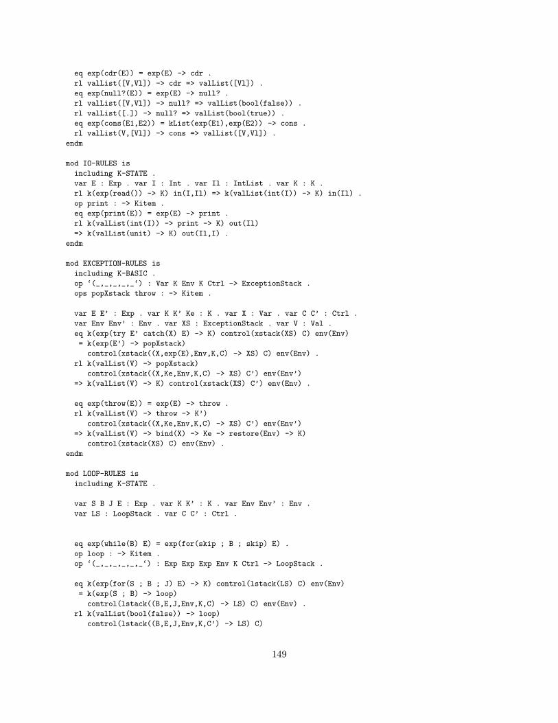
eq exp(cdr(E)) = exp(E) -> cdr .

rl valList([V,Vl]) -> cdr => valList([Vl]) .

eq exp(null?(E)) = exp(E) -> null? .

rl valList([V,Vl]) -> null? => valList(bool(false)) .

rl valList([.]) -> null? => valList(bool(true)) .

eq exp(cons(E1,E2)) = kList(exp(E1),exp(E2)) -> cons .

rl valList(V,[Vl]) -> cons => valList([V,Vl]) .

endm

mod IO-RULES is

including K-STATE .

var E : Exp . var I : Int . var Il : IntList . var K : K .

rl k(exp(read()) -> K) in(I,Il) => k(valList(int(I)) -> K) in(Il) .

op print : -> Kitem .

eq exp(print(E)) = exp(E) -> print .

rl k(valList(int(I)) -> print -> K) out(Il)

=> k(valList(unit) -> K) out(Il,I) .

endm

mod EXCEPTION-RULES is

including K-BASIC .

op ‘(_,_,_,_,_‘) : Var K Env K Ctrl -> ExceptionStack .

ops popXstack throw : -> Kitem .

var E E’ : Exp . var K K’ Ke : K . var X : Var . var C C’ : Ctrl .

var Env Env’ : Env . var XS : ExceptionStack . var V : Val .

eq k(exp(try E’ catch(X) E) -> K) control(xstack(XS) C) env(Env)

= k(exp(E’) -> popXstack)

control(xstack((X,exp(E),Env,K,C) -> XS) C) env(Env) .

rl k(valList(V) -> popXstack)

control(xstack((X,Ke,Env,K,C) -> XS) C’) env(Env’)

=> k(valList(V) -> K) control(xstack(XS) C’) env(Env) .

eq exp(throw(E)) = exp(E) -> throw .

rl k(valList(V) -> throw -> K’)

control(xstack((X,Ke,Env,K,C) -> XS) C’) env(Env’)

=> k(valList(V) -> bind(X) -> Ke -> restore(Env) -> K)

control(xstack(XS) C) env(Env) .

endm

mod LOOP-RULES is

including K-STATE .

var S B J E : Exp . var K K’ : K . var Env Env’ : Env .

var LS : LoopStack . var C C’ : Ctrl .

eq exp(while(B) E) = exp(for(skip ; B ; skip) E) .

op loop : -> Kitem .

op ‘(_,_,_,_,_,_‘) : Exp Exp Exp Env K Ctrl -> LoopStack .

eq k(exp(for(S ; B ; J) E) -> K) control(lstack(LS) C) env(Env)

= k(exp(S ; B) -> loop)

control(lstack((B,E,J,Env,K,C) -> LS) C) env(Env) .

rl k(valList(bool(false)) -> loop)

control(lstack((B,E,J,Env,K,C’) -> LS) C)

149

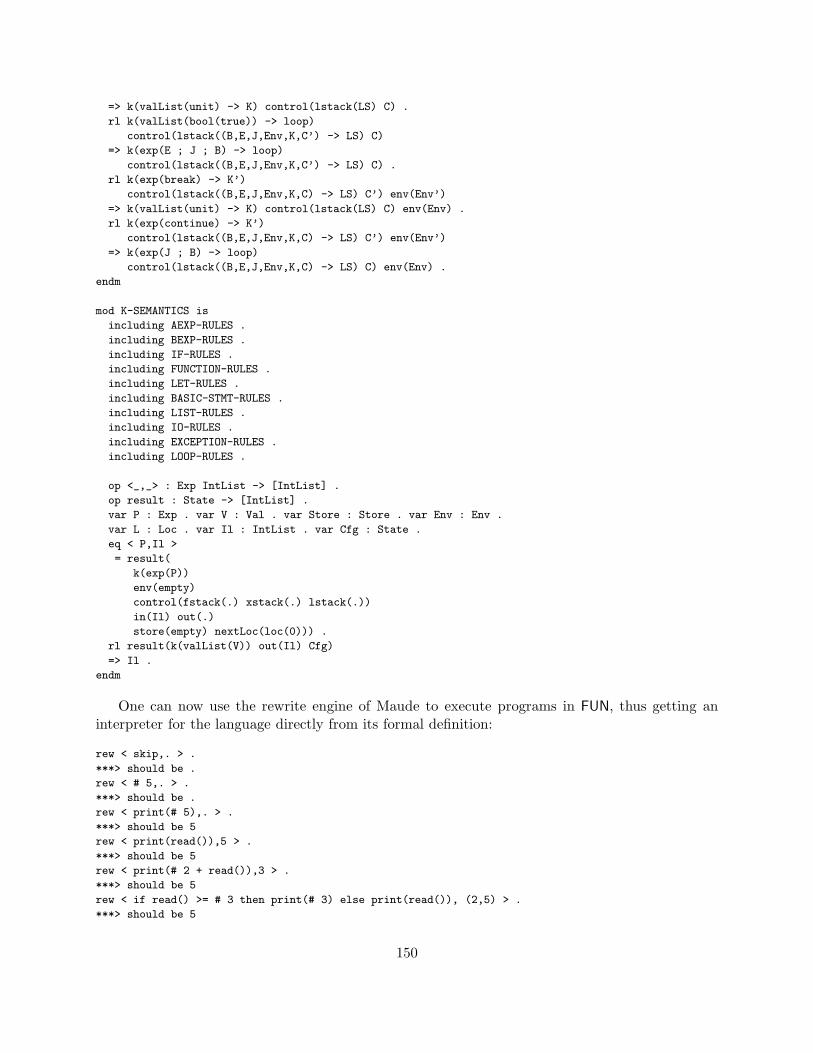
=> k(valList(unit) -> K) control(lstack(LS) C) .

rl k(valList(bool(true)) -> loop)

control(lstack((B,E,J,Env,K,C’) -> LS) C)

=> k(exp(E ; J ; B) -> loop)

control(lstack((B,E,J,Env,K,C’) -> LS) C) .

rl k(exp(break) -> K’)

control(lstack((B,E,J,Env,K,C) -> LS) C’) env(Env’)

=> k(valList(unit) -> K) control(lstack(LS) C) env(Env) .

rl k(exp(continue) -> K’)

control(lstack((B,E,J,Env,K,C) -> LS) C’) env(Env’)

=> k(exp(J ; B) -> loop)

control(lstack((B,E,J,Env,K,C) -> LS) C) env(Env) .

endm

mod K-SEMANTICS is

including AEXP-RULES .

including BEXP-RULES .

including IF-RULES .

including FUNCTION-RULES .

including LET-RULES .

including BASIC-STMT-RULES .

including LIST-RULES .

including IO-RULES .

including EXCEPTION-RULES .

including LOOP-RULES .

op <_,_> : Exp IntList -> [IntList] .

op result : State -> [IntList] .

var P : Exp . var V : Val . var Store : Store . var Env : Env .

var L : Loc . var Il : IntList . var Cfg : State .

eq < P,Il >

= result(

k(exp(P))

env(empty)

control(fstack(.) xstack(.) lstack(.))

in(Il) out(.)

store(empty) nextLoc(loc(0))) .

rl result(k(valList(V)) out(Il) Cfg)

=> Il .

endm

One can now use the rewrite engine of Maude to execute programs in FUN, thus getting aninterpreter for the language directly from its formal definition:

rew < skip,. > .

***> should be .

rew < # 5,. > .

***> should be .

rew < print(# 5),. > .

***> should be 5

rew < print(read()),5 > .

***> should be 5

rew < print(# 2 + read()),3 > .

***> should be 5

rew < if read() >= # 3 then print(# 3) else print(read()), (2,5) > .

***> should be 5

150

rew < if read() >= # 3 then print(# 5) else print(read()), (4,2) > .

***> should be 5

rew < let(x,# 5,print(x)),. > .

***> should be 5

rew < (fun x -> print(x))(# 5),. > .

***> should be 5

rew < letrec(f,fun x -> (if x == # 0 then # 0 else (# 1 + (f(x /

# 2)))),

print(f(# 31))),. > .

***> should be 5

rew < letrec(’max,fun l ->

((if null?(cdr(l)) then return(car(l))) ;

let(x,(’max(cdr(l))),

((if (x <= car(l)) then return(car(l))) ;

return(x)))),

print(’max([# 1,# 3,# 5,# 2,# 4,# 0,# -1,# -9]))),. > .

***> should be 5

rew < letrec(’len,fun l -> (if null?(l) then # 0 else (# 1 +

(’len(cdr(l))))),

print(’len(cons(# 3,[# 4,# 7,# 9,# 2])))),. > .

***> should be 5

rew < (try throw(read()) catch(x) print(x)),5 > .

***> should be 5

rew < (try let((x,y),(read(),read()),if y == # 0 then throw(x) else

print(x / y)) catch(x) print(x)),(15,3) > .

***> should be 5

rew < (try let((x,y),(read(),read()),if y == # 0 then throw(x) else

print(x / y)) catch(x) print(x)),(5,0) > .

***> should be 5

rew < let ((x,y),(read(),read()),

((while(not(y == # 0))

((x := (x % y)) ;

(x := (x + y)) ;

(y := (x - y)) ;

(x := (x - y)) )) ;

print(x))),(25,15) > .

***> should be 5

rew < let ((x,y),(read(),read()),

((for(skip ; not(y == # 0) ; ((x := (x % y)) ;

(x := (x + y)) ;

(y := (x - y)) ;

(x := (x - y)) )) skip) ; print(x))),(35,25) > .

***> should be 5

rew < let (x,read(),for( skip ; true ; x := read()) ((if x <= # 0 then

continue) ; print(x) ; break)),(-2,0,-3,-7,5,-4,30,2) > .

***> should be 5

G Definition of Full FUN in Maude

In this appendix we show the Maude-ified version of the full FUN language, whose K-definition isshown in Figure 9.

fmod SYNTAX is

151

including INT .

including QID .

--- Var

sort Var .

subsort Qid < Var .

ops a b c d e f g h i j k l m n o p q r t u v x y z : -> Var [format (g o)] .

sort Exp .

subsort Var < Exp .

op #_ : Int -> Exp [prec 30 format (b r o)] .

ops _+_ _-_ : Exp Exp -> Exp [prec 33 gather (E e) format (d b o d)] .

ops _*_ _/_ _%_ : Exp Exp -> Exp

[prec 32 gather (E e) format (d b o d)] .

ops true false : -> Exp [format (r o)] .

ops _<=_ _>=_ _==_ : Exp Exp -> Exp [prec 37 format (d b o d)] .

op _and_ : Exp Exp -> Exp [prec 55 format (d b o d)] .

op _or_ : Exp Exp -> Exp [prec 57 format (d b o d)] .

op not_ : Exp -> Exp [prec 53 format (b o d)] .

op skip : -> Exp [format (b o)] .

op if_then_ : Exp Exp -> Exp

[prec 70 format (b o bn+i o+ --)] .

op if_then_else_ : Exp Exp Exp -> Exp

[prec 70 format (b o bn+i o+ bn-i o+ --)] .

sort VarList ExpList .

op _,_ : VarList VarList -> VarList [assoc id: .] .

op . : -> VarList .

op _,_ : ExpList ExpList -> ExpList [ditto] .

subsort Var < VarList Exp < ExpList .

op fun_->_ : VarList Exp -> Exp [format (b o b no++i n--)] .

op _‘(_‘) : Exp ExpList -> Exp [prec 60 format(d b o b o)] .

op return : Exp -> Exp [format (b o)] .

ops let letrec : VarList ExpList Exp -> Exp [format (b o)] .

op _;_ : Exp Exp -> Exp [gather (e E) prec 80 format (d b noi d)] .

op _:=_ : Var Exp -> Exp [format (d b o d)] .

op ‘[_‘] : ExpList -> Exp [format (b o b o)] .

ops car cdr null? : Exp -> Exp [format (b o)] .

op cons : Exp Exp -> Exp [format (b o)] .

op read‘(‘) : -> Exp [format (b d d o)] .

op print : Exp -> Exp [format (b o)] .

op try_catch‘(_‘)_ : Exp Var Exp -> Exp [format (b o b d o b o d)] .

op throw : Exp -> Exp [format (b o)] .

op while‘(_‘)_ : Exp Exp -> Exp [format (b d o b no++i --)] .

op for‘(_;_;_‘)_ : Exp Exp Exp Exp -> Exp

[format (b d o b o b o b no++i --)] .

152

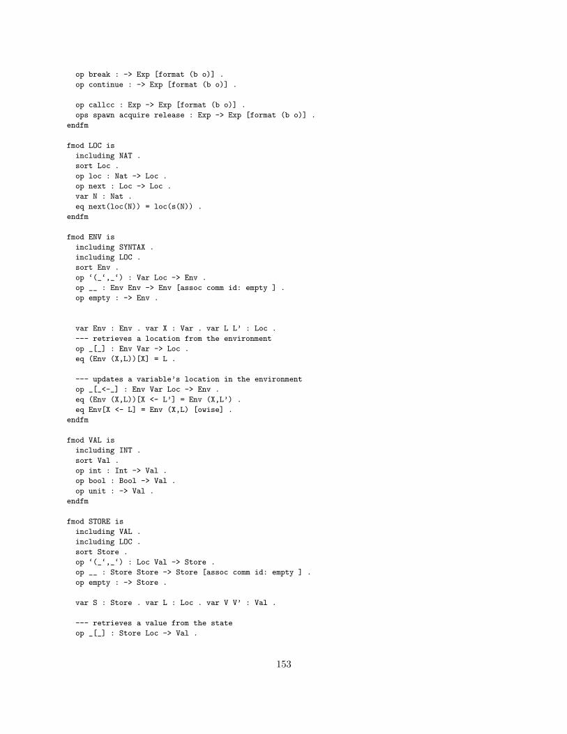
op break : -> Exp [format (b o)] .

op continue : -> Exp [format (b o)] .

op callcc : Exp -> Exp [format (b o)] .

ops spawn acquire release : Exp -> Exp [format (b o)] .

endfm

fmod LOC is

including NAT .

sort Loc .

op loc : Nat -> Loc .

op next : Loc -> Loc .

var N : Nat .

eq next(loc(N)) = loc(s(N)) .

endfm

fmod ENV is

including SYNTAX .

including LOC .

sort Env .

op ‘(_‘,_‘) : Var Loc -> Env .

op __ : Env Env -> Env [assoc comm id: empty ] .

op empty : -> Env .

var Env : Env . var X : Var . var L L’ : Loc .

--- retrieves a location from the environment

op _[_] : Env Var -> Loc .

eq (Env (X,L))[X] = L .

--- updates a variable’s location in the environment

op _[_<-_] : Env Var Loc -> Env .

eq (Env (X,L))[X <- L’] = Env (X,L’) .

eq Env[X <- L] = Env (X,L) [owise] .

endfm

fmod VAL is

including INT .

sort Val .

op int : Int -> Val .

op bool : Bool -> Val .

op unit : -> Val .

endfm

fmod STORE is

including VAL .

including LOC .

sort Store .

op ‘(_‘,_‘) : Loc Val -> Store .

op __ : Store Store -> Store [assoc comm id: empty ] .

op empty : -> Store .

var S : Store . var L : Loc . var V V’ : Val .

--- retrieves a value from the state

op _[_] : Store Loc -> Val .

153

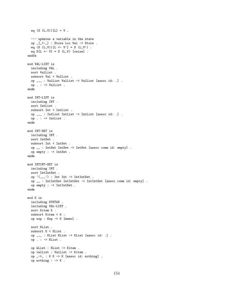
eq (S (L,V))[L] = V .

--- updates a variable in the state

op _[_<-_] : Store Loc Val -> Store .

eq (S (L,V))[L <- V’] = S (L,V’) .

eq S[L <- V] = S (L,V) [owise] .

endfm

mod VAL-LIST is

including VAL .

sort ValList .

subsort Val < ValList .

op _,_ : ValList ValList -> ValList [assoc id: .] .

op . : -> ValList .

endm

mod INT-LIST is

including INT .

sort IntList .

subsort Int < IntList .

op _,_ : IntList IntList -> IntList [assoc id: .] .

op . : -> IntList .

endm

mod INT-SET is

including INT .

sort IntSet .

subsort Int < IntSet .

op __ : IntSet IntSet -> IntSet [assoc comm id: empty] .

op empty : -> IntSet .

endm

mod INTINT-SET is

including INT .

sort IntIntSet .

op ‘(_,_‘) : Int Int -> IntIntSet .

op __ : IntIntSet IntIntSet -> IntIntSet [assoc comm id: empty] .

op empty : -> IntIntSet .

endm

mod K is

including SYNTAX .

including VAL-LIST .

sort Kitem K .

subsort Kitem < K .

op exp : Exp -> K [memo] .

sort KList .

subsort K < KList .

op _,_ : KList KList -> KList [assoc id: .] .

op . : -> KList .

op kList : KList -> Kitem .

op valList : ValList -> Kitem .

op _->_ : K K -> K [assoc id: nothing] .

op nothing : -> K .

154

endm

mod STACKS is

sorts FunctionStack ExceptionStack LoopStack .

op _->_ : FunctionStack FunctionStack -> FunctionStack [assoc id: .] .

op . : -> FunctionStack .

op _->_ : ExceptionStack ExceptionStack -> ExceptionStack [assoc id:

.] .

op . : -> ExceptionStack .

op _->_ : LoopStack LoopStack -> LoopStack [assoc id: .] .

op . : -> LoopStack .

endm

mod CONTROL is

including STACKS .

sort Ctrl .

op __ : Ctrl Ctrl -> Ctrl [assoc comm id: .] .

op . : -> Ctrl .

op fstack : FunctionStack -> Ctrl .

op xstack : ExceptionStack -> Ctrl .

op lstack : LoopStack -> Ctrl .

endm

mod K-THREAD-STATE is

including CONTROL .

including ENV .

including K .

including INTINT-SET .

sort ThreadState .

op __ : ThreadState ThreadState -> ThreadState [assoc comm id: .] .

op . : -> ThreadState .

op k : K -> ThreadState .

op env : Env -> ThreadState .

op control : Ctrl -> ThreadState .

op holds : IntIntSet -> ThreadState .

endm

mod K-STATE is

including INT-LIST .

including INT-SET .

including STORE .

including K-THREAD-STATE .

sort State .

op __ : State State -> State [assoc comm id: .] .

op . : -> State .

ops in out : IntList -> State .

op store : Store -> State .

op nextLoc : Loc -> State .

op thread : ThreadState -> State .

op busy : IntSet -> State .

var E : Exp . var Env : Env .

op newThread : Exp Env -> State .

eq newThread(E,Env) = thread(k(exp(E)) env(Env)

155

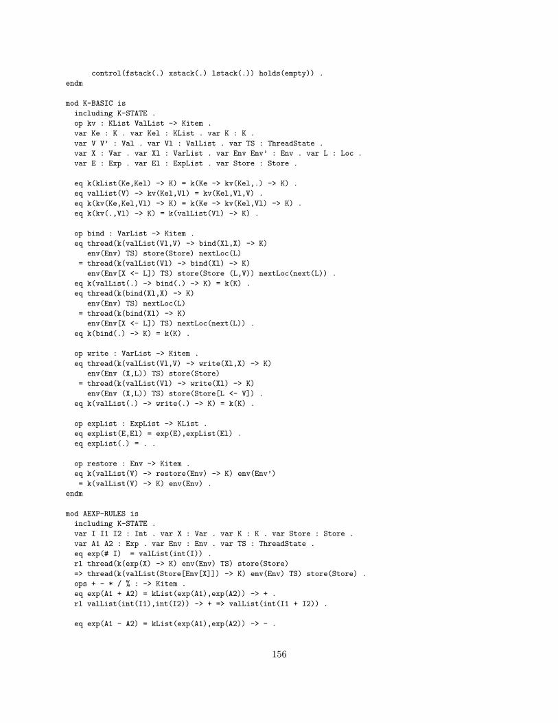
control(fstack(.) xstack(.) lstack(.)) holds(empty)) .

endm

mod K-BASIC is

including K-STATE .

op kv : KList ValList -> Kitem .

var Ke : K . var Kel : KList . var K : K .

var V V’ : Val . var Vl : ValList . var TS : ThreadState .

var X : Var . var Xl : VarList . var Env Env’ : Env . var L : Loc .

var E : Exp . var El : ExpList . var Store : Store .

eq k(kList(Ke,Kel) -> K) = k(Ke -> kv(Kel,.) -> K) .

eq valList(V) -> kv(Kel,Vl) = kv(Kel,Vl,V) .

eq k(kv(Ke,Kel,Vl) -> K) = k(Ke -> kv(Kel,Vl) -> K) .

eq k(kv(.,Vl) -> K) = k(valList(Vl) -> K) .

op bind : VarList -> Kitem .

eq thread(k(valList(Vl,V) -> bind(Xl,X) -> K)

env(Env) TS) store(Store) nextLoc(L)

= thread(k(valList(Vl) -> bind(Xl) -> K)

env(Env[X <- L]) TS) store(Store (L,V)) nextLoc(next(L)) .

eq k(valList(.) -> bind(.) -> K) = k(K) .

eq thread(k(bind(Xl,X) -> K)

env(Env) TS) nextLoc(L)

= thread(k(bind(Xl) -> K)

env(Env[X <- L]) TS) nextLoc(next(L)) .

eq k(bind(.) -> K) = k(K) .

op write : VarList -> Kitem .

eq thread(k(valList(Vl,V) -> write(Xl,X) -> K)

env(Env (X,L)) TS) store(Store)

= thread(k(valList(Vl) -> write(Xl) -> K)

env(Env (X,L)) TS) store(Store[L <- V]) .

eq k(valList(.) -> write(.) -> K) = k(K) .

op expList : ExpList -> KList .

eq expList(E,El) = exp(E),expList(El) .

eq expList(.) = . .

op restore : Env -> Kitem .

eq k(valList(V) -> restore(Env) -> K) env(Env’)

= k(valList(V) -> K) env(Env) .

endm

mod AEXP-RULES is

including K-STATE .

var I I1 I2 : Int . var X : Var . var K : K . var Store : Store .

var A1 A2 : Exp . var Env : Env . var TS : ThreadState .

eq exp(# I) = valList(int(I)) .

rl thread(k(exp(X) -> K) env(Env) TS) store(Store)

=> thread(k(valList(Store[Env[X]]) -> K) env(Env) TS) store(Store) .

ops + - * / % : -> Kitem .

eq exp(A1 + A2) = kList(exp(A1),exp(A2)) -> + .

rl valList(int(I1),int(I2)) -> + => valList(int(I1 + I2)) .

eq exp(A1 - A2) = kList(exp(A1),exp(A2)) -> - .

156

rl valList(int(I1),int(I2)) -> - => valList(int(_-_(I1,I2))) .

eq exp(A1 * A2) = kList(exp(A1),exp(A2)) -> * .

rl valList(int(I1),int(I2)) -> * => valList(int(I1 * I2)) .

eq exp(A1 / A2) = kList(exp(A1),exp(A2)) -> / .

crl valList(int(I1),int(I2)) -> / => valList(int(I1 quo I2))

if I2 =/= 0 .

eq exp(A1 % A2) = kList(exp(A1),exp(A2)) -> % .

crl valList(int(I1),int(I2)) -> % => valList(int(I1 rem I2))

if I2 =/= 0 .

endm

mod BEXP-RULES is

including K-STATE .

var X : Var . var Store : Store . var B B1 B2 : Exp .

var A1 A2 : Exp . var I1 I2 : Int . var T T1 T2 : Bool .

eq exp(true) = valList(bool(true)) .

eq exp(false) = valList(bool(false)) .

ops <= >= == and or not : -> Kitem .

eq exp(A1 <= A2) = kList(exp(A1),exp(A2)) -> <= .

rl valList(int(I1),int(I2)) -> <= => valList(bool(I1 <= I2)) .

eq exp(A1 >= A2) = kList(exp(A1),exp(A2)) -> >= .

rl valList(int(I1),int(I2)) -> >= => valList(bool(I1 >= I2)) .

eq exp(A1 == A2) = kList(exp(A1),exp(A2)) -> == .

rl valList(int(I1),int(I2)) -> == => valList(bool(I1 == I2)) .

eq exp(B1 and B2) = kList(exp(B1),exp(B2)) -> and .

rl valList(bool(T1),bool(T2)) -> and => valList(bool(T1 and T2)) .

eq exp(B1 or B2) = kList(exp(B1),exp(B2)) -> or .

rl valList(bool(T1),bool(T2)) -> or => valList(bool(T1 or T2)) .

eq exp(not B) = exp(B) -> not .

rl valList(bool(T)) -> not => valList(bool(not T)) .

endm

mod IF-RULES is

including K-STATE .

op if : K K -> Kitem .

var E E1 E2 : Exp . var K K1 K2 : K .

eq exp(if E then E1) = exp(if E then E1 else skip) .

eq exp(if E then E1 else E2) = exp(E) -> if(exp(E1),exp(E2)) .

rl k(valList(bool(true)) -> if(K1,K2) -> K) => k(K1 -> K) .

rl k(valList(bool(false)) -> if(K1,K2) -> K) => k(K2 -> K) .

endm

mod FUNCTION-RULES is

including K-BASIC .

op closure : VarList K Env -> Val .

var Xl : VarList . var E : Exp . var El : ExpList . var X : Var .

var Env Env’ : Env . var V : Val . var Vl : ValList . var K K’ : K .

var Store : Store . var L : Loc . var FS : FunctionStack .

157

var C C’ : Ctrl .

eq k(exp(fun Xl -> E) -> K) env(Env)

= k(valList(closure(Xl,exp(E),Env)) -> K) env(Env) .

op app : -> Kitem .

eq exp(E(El)) = kList(exp(E),expList(El)) -> app .

op ‘(_,_,_‘) : K Env Ctrl -> FunctionStack .

ops popFstack return : -> Kitem .

rl k(valList(closure(Xl,K,Env),Vl) -> app -> K’)

control(fstack(FS) C) env(Env’)

=> k(valList(Vl) -> bind(Xl) -> K -> popFstack)

control(fstack((K’,Env’,C) -> FS) C) env(Env) .

eq k(valList(V) -> popFstack)

control(fstack((K,Env,C’) -> FS) C) env(Env’)

= k(valList(V) -> K) control(fstack(FS) C) env(Env) .

eq exp(return(E)) = exp(E) -> return .

eq k(valList(V) -> return -> K’)

control(fstack((K,Env,C) -> FS) C’) env(Env’)

= k(valList(V) -> K) control(fstack(FS) C) env(Env) .

endm

mod LET-RULES is

including K-BASIC .

var Env Env’ : Env . var K : K . var Xl : VarList . var El : ExpList .

var E : Exp .

rl k(exp(let(Xl,El,E)) -> K) env(Env)

=> k(kList(expList(El)) -> bind(Xl) -> exp(E) -> restore(Env) -> K)

env(Env) .

rl k(exp(letrec(Xl,El,E)) -> K) env(Env)

=> k(bind(Xl) -> kList(expList(El)) -> write(Xl) -> exp(E)

-> restore(Env) -> K) env(Env) .

endm

mod BASIC-STMT-RULES is

including K-BASIC .

eq exp(skip) = valList(unit) .

op ; : -> Kitem .

var E E1 E2 : Exp . var V1 V2 : Val . var X : Var .

eq exp(E1 ; E2) = kList(exp(E1),exp(E2)) -> ; .

rl valList(V1,V2) -> ; => valList(V2) .

eq exp(X := E) = exp(E) -> write(X) -> valList(unit) .

endm

mod LIST-RULES is

including K-BASIC .

ops ‘[‘] car cdr null? cons : -> Kitem .

var El : ExpList . var Vl : ValList . var E E1 E2 : Exp .

var V : Val .

eq exp([El]) = kList(expList(El)) -> [] .

op ‘[_‘] : ValList -> Val .

eq valList(Vl) -> [] = valList([Vl]) .

eq exp(car(E)) = exp(E) -> car .

rl valList([V,Vl]) -> car => valList(V) .

158

eq exp(cdr(E)) = exp(E) -> cdr .

rl valList([V,Vl]) -> cdr => valList([Vl]) .

eq exp(null?(E)) = exp(E) -> null? .

rl valList([V,Vl]) -> null? => valList(bool(false)) .

rl valList([.]) -> null? => valList(bool(true)) .

eq exp(cons(E1,E2)) = kList(exp(E1),exp(E2)) -> cons .

rl valList(V,[Vl]) -> cons => valList([V,Vl]) .

endm

mod IO-RULES is

including K-STATE .

var E : Exp . var I : Int . var Il : IntList . var K : K .

var TS : ThreadState .

rl thread(k(exp(read()) -> K) TS) in(I,Il)

=> thread(k(valList(int(I)) -> K) TS) in(Il) .

op print : -> Kitem .

eq exp(print(E)) = exp(E) -> print .

rl thread(k(valList(int(I)) -> print -> K) TS) out(Il)

=> thread(k(valList(unit) -> K) TS) out(Il,I) .

endm

mod EXCEPTION-RULES is

including K-BASIC .

op ‘(_,_,_,_,_‘) : Var K Env K Ctrl -> ExceptionStack .

ops popXstack throw : -> Kitem .

var E E’ : Exp . var K K’ Ke : K . var X : Var . var C C’ : Ctrl .

var Env Env’ : Env . var XS : ExceptionStack . var V : Val .

eq k(exp(try E’ catch(X) E) -> K) control(xstack(XS) C) env(Env)

= k(exp(E’) -> popXstack)

control(xstack((X,exp(E),Env,K,C) -> XS) C) env(Env) .

rl k(valList(V) -> popXstack)

control(xstack((X,Ke,Env,K,C) -> XS) C’) env(Env’)

=> k(valList(V) -> K) control(xstack(XS) C’) env(Env) .

eq exp(throw(E)) = exp(E) -> throw .

rl k(valList(V) -> throw -> K’)

control(xstack((X,Ke,Env,K,C) -> XS) C’) env(Env’)

=> k(valList(V) -> bind(X) -> Ke -> restore(Env) -> K)

control(xstack(XS) C) env(Env) .

endm

mod LOOP-RULES is

including K-STATE .

var S B J E : Exp . var K K’ : K . var Env Env’ : Env .

var LS : LoopStack . var C C’ : Ctrl .

eq exp(while(B) E) = exp(for(skip ; B ; skip) E) .

op loop : -> Kitem .

op ‘(_,_,_,_,_,_‘) : Exp Exp Exp Env K Ctrl -> LoopStack .

eq k(exp(for(S ; B ; J) E) -> K) control(lstack(LS) C) env(Env)

= k(exp(S ; B) -> loop)

control(lstack((B,E,J,Env,K,C) -> LS) C) env(Env) .

159

rl k(valList(bool(false)) -> loop)

control(lstack((B,E,J,Env,K,C’) -> LS) C)

=> k(valList(unit) -> K) control(lstack(LS) C) .

rl k(valList(bool(true)) -> loop)

control(lstack((B,E,J,Env,K,C’) -> LS) C)

=> k(exp(E ; J ; B) -> loop)

control(lstack((B,E,J,Env,K,C’) -> LS) C) .

rl k(exp(break) -> K’)

control(lstack((B,E,J,Env,K,C) -> LS) C’) env(Env’)

=> k(valList(unit) -> K) control(lstack(LS) C) env(Env) .

rl k(exp(continue) -> K’)

control(lstack((B,E,J,Env,K,C) -> LS) C’) env(Env’)

=> k(exp(J ; B) -> loop)

control(lstack((B,E,J,Env,K,C) -> LS) C) env(Env) .

endm

mod CALLCC-RULES is

including FUNCTION-RULES .

op callcc : -> Kitem .

op cc : K Ctrl Env -> Val .

var E : Exp . var V : Val . var K K’ : K . var Env Env’ : Env .

var C C’ : Ctrl .

eq exp(callcc(E)) = exp(E) -> callcc .

rl k(valList(V) -> callcc -> K) control(C) env(Env)

=> k(valList(V,cc(K,C,Env)) -> app -> K) control(C) env(Env) .

rl k(valList(cc(K,C,Env),V) -> app -> K’) control(C’) env(Env’)

=> k(valList(V) -> K) control(C) env(Env) .

endm

mod THREAD-RULES is

including K-STATE .

var V : Val . var TS : ThreadState . var E : Exp . var Env : Env .

var I : Int . var N : Nat . var Is : IntSet . var LCs : IntIntSet .

var K : K .

rl thread(k(exp(spawn(E)) -> K) env(Env) TS)

=> thread(k(valList(unit) -> K) env(Env) TS) newThread(E,Env) .

rl thread(k(valList(V)) holds(LCs) TS) busy(Is)

=> busy(Is - LCs) .

ops acquire release : -> Kitem .

eq exp(acquire(E)) = exp(E) -> acquire .

rl k(valList(int(I)) -> acquire -> K) holds((I,N) LCs)

=> k(valList(unit) -> K) holds((I,s(N)) LCs) .

crl thread(k(valList(int(I)) -> acquire -> K) holds(LCs) TS) busy(Is)

=> thread(k(valList(unit) -> K) holds((I,0) LCs) TS) busy(Is I)

if not(I in Is) .

op _in_ : Int IntSet -> Bool .

eq I in I Is = true .

eq I in Is = false [owise] .

eq exp(release(E)) = exp(E) -> release .

rl k(valList(int(I)) -> release -> K) holds((I,s(N)) LCs)

=> k(valList(unit) -> K) holds((I,N) LCs) .

rl thread(k(valList(int(I)) -> release -> K) holds((I,0) LCs) TS)

160

busy(Is I)

=> thread(k(valList(unit) -> K) holds(LCs) TS) busy(Is) .

op _-_ : IntSet IntIntSet -> IntSet .

eq (I Is) - ((I,N) LCs) = Is - LCs .

eq Is - LCs = Is [owise] .

endm

mod K-SEMANTICS is

including AEXP-RULES .

including BEXP-RULES .

including IF-RULES .

including FUNCTION-RULES .

including LET-RULES .

including BASIC-STMT-RULES .

including LIST-RULES .

including IO-RULES .

including EXCEPTION-RULES .

including LOOP-RULES .

including CALLCC-RULES .

including THREAD-RULES .

op <_,_> : Exp IntList -> [IntList] .

op result : State -> [IntList] .

var P : Exp . var Store : Store . var Is : IntSet .

var L : Loc . var Il Il’ : IntList . var Cfg : State .

var TS : ThreadState .

eq < P,Il >

= result(

newThread(P,empty)

in(Il) out(.)

store(empty) nextLoc(loc(0)) busy(empty)) .

rl result(busy(Is) in(Il’) out(Il) store(Store) nextLoc(L))

=> Il .

endm

Like for the Maude definition of sequential FUN in Appendix F, one can now use the rewriteengine to execute programs in FUN, thus getting an interpreter for the language directly from itsformal definition. All the examples in Appendix F can be executed, plus many others involvingcallcc and threads. Also, one can use Maude’s generic formal analysis tools to obtain correspondingformal analysis tools for FUN. For example, the two search commands below invoke the reachabilityanalysis capability of Maude:

rew <

let(’+,(fun (x,y) -> print(x + y)),

(callcc((fun k -> (k(’+))))(read(),read()))),

(2, 3) > .

***> sum using callcc - should print 5

search < let(x,# 0,(spawn(x := (x + # 2)) ; spawn(x := (x + # 3)) ;

print(x))),. >

=>! I:Int .

***> should give 4 solutions, one of them 5 : dataraces & print may not wait

search < let((x,’t1,’t2),(# 0,# 0,# 0),

(spawn((x := (x + # 2)); (’t1 := # 1)) ;

161

spawn((x := (x + # 3)) ; (’t2 := # 1)) ;

(while(not((’t1 + ’t2) == # 2)) skip) ;

print(x)

)),. >

=>! I:Int .

***> should give 3 solutions, one of them 5 : dataraces, print should wait

search < let((x,t),(# 0,# 0),

(spawn(acquire(# 0) ; (x := (x + # 2)); (t := (t + # 1)) ;

release(# 0)) ;

spawn(acquire(# 0) ; (x := (x + # 3)) ; (t := (t + # 1)) ;

release(# 0)) ;

(while(not(t == # 2)) skip) ;

print(x)

)),. >

=>! I:Int .

***> should give 1 solution: 5

Many more examples of formal analysis of concurrent programs are shown in Section 10.

162