JT 305 Advanced Computational Methods · PDF fileJawaharlal Nehru Centre for Advanced Scienti...
70
CONTENTS 1 JT 305 Advanced Computational Methods Srikanth Sastry Jawaharlal Nehru Centre for Advanced Scientific Research Bengaluru,560064 [email protected] Course URL: http://www.jncasr.ac.in/sastry/jt305 Tutor: Anshul D S Parmar [email protected] Contents 1 Course Outline 3 2 Introdution 5 3 Statistical Mechanics - Basic Concepts 6 4 Monte Carlo Methods - Basic Principles 9 4.1 Monte Carlo Sampling ................................ 9 4.2 The Metropolis Algorithm .............................. 11 4.3 Detailed Balance ................................... 14 4.4 Random Numbers ................................... 16 5 Monte Carlo simulation of lattice and off-lattice systems 19 5.1 Monte Carlo simulations: Examples ......................... 19 5.2 Monte Carlo simulations in various ensembles ................... 26 6 Molecular dynamics simulations - basic principles 30 6.1 Special Cases: Long range forces, Event driven MD, Molecular systems ..... 34 6.2 Long range interactions: Ewald sum ......................... 37 7 Molecular dynamics in various ensembles 45 7.1 Molecular Dynamics in the (N,V,T ) ensemble: ................... 45 7.2 Molecular Dynamics in the (N,P,T ) ensemble: ................... 47 8 Analysis of data: Statistics and Error Estimation 48 9 Histogram Methods 49 9.1 Umbrella Sampling .................................. 50 9.2 Histogram Reweighting or Multi-Histogram Method ................ 52
Transcript of JT 305 Advanced Computational Methods · PDF fileJawaharlal Nehru Centre for Advanced Scienti...
CONTENTS 1
JT 305 Advanced Computational MethodsSrikanth Sastry
Jawaharlal Nehru Centre for Advanced Scientific ResearchBengaluru,[email protected]
Course URL: http://www.jncasr.ac.in/sastry/jt305
Tutor: Anshul D S [email protected]
Contents
1 Course Outline 3
2 Introdution 5
3 Statistical Mechanics - Basic Concepts 6
4 Monte Carlo Methods - Basic Principles 9
4.1 Monte Carlo Sampling . . . . . . . . . . . . . . . . . . . . . . . . . . . . . . . . 9
4.2 The Metropolis Algorithm . . . . . . . . . . . . . . . . . . . . . . . . . . . . . . 11
4.3 Detailed Balance . . . . . . . . . . . . . . . . . . . . . . . . . . . . . . . . . . . 14
4.4 Random Numbers . . . . . . . . . . . . . . . . . . . . . . . . . . . . . . . . . . . 16
5 Monte Carlo simulation of lattice and off-lattice systems 19
5.1 Monte Carlo simulations: Examples . . . . . . . . . . . . . . . . . . . . . . . . . 19
5.2 Monte Carlo simulations in various ensembles . . . . . . . . . . . . . . . . . . . 26
6 Molecular dynamics simulations - basic principles 30
6.1 Special Cases: Long range forces, Event driven MD, Molecular systems . . . . . 34
6.2 Long range interactions: Ewald sum . . . . . . . . . . . . . . . . . . . . . . . . . 37
7 Molecular dynamics in various ensembles 45
7.1 Molecular Dynamics in the (N, V, T ) ensemble: . . . . . . . . . . . . . . . . . . . 45
7.2 Molecular Dynamics in the (N,P, T ) ensemble: . . . . . . . . . . . . . . . . . . . 47
8 Analysis of data: Statistics and Error Estimation 48
9 Histogram Methods 49
9.1 Umbrella Sampling . . . . . . . . . . . . . . . . . . . . . . . . . . . . . . . . . . 50
9.2 Histogram Reweighting or Multi-Histogram Method . . . . . . . . . . . . . . . . 52

CONTENTS 2
9.3 Wang-Landau Algorithm . . . . . . . . . . . . . . . . . . . . . . . . . . . . . . . 53
10 Free Energy calculation and phase equilibria 54
10.1 Thermodynamic Integration: . . . . . . . . . . . . . . . . . . . . . . . . . . . . . 54
10.2 Widom Insertion Method for Chemical Potential: . . . . . . . . . . . . . . . . . 55
10.3 Phase Equilibria: The Gibbs Ensemble Method: . . . . . . . . . . . . . . . . . . 56
10.4 Gibbs-Duhem Integration . . . . . . . . . . . . . . . . . . . . . . . . . . . . . . 57
11 Optimization, biased and accelerated sampling 59
11.1 Simulated Annealing . . . . . . . . . . . . . . . . . . . . . . . . . . . . . . . . . 59
11.2 Parallel Tempering: . . . . . . . . . . . . . . . . . . . . . . . . . . . . . . . . . . 60
11.3 Configurational Bias Monte Carlo: . . . . . . . . . . . . . . . . . . . . . . . . . . 61
11.4 Hybrid Monte Carlo . . . . . . . . . . . . . . . . . . . . . . . . . . . . . . . . . 63
11.5 Cluster algorithms . . . . . . . . . . . . . . . . . . . . . . . . . . . . . . . . . . 63
12 Rare Events 67
13 Critical Behavior 68
14 Non-Equilibrium Processes 70

1 COURSE OUTLINE 3
1 Course Outline
Class Times: Thurs 2:00 PM - 3:30 PM, 5:00 - 6:30 PM, January - April 2016 Semester.
Venue: TUE-CMS Instructional Class Room
Course Structure
The lectures will cover the following topics.
1 Statistical Mechanics - Basic Concepts
2 The Monte Carlo method for sampling and importance sampling.
3 Monte Carlo simulation of lattice and off-lattice systems.
4 Molecular dynamics simulations - basic principles
5 Molecular dynamics simulations in various ensembles, boundary conditions [(N,V,E),
(N,V,T), (N,P,T), Parrinello-Rahman]
6 Analysis of data: Statistics, Error Estimation
7 Histogram Methods (umbrella sampling, histogram reweighting, Wang-Landau sampling).
8 Free energies and phase equilibria (thermodynamic integration, Gibbs ensemble, Gibbs-
Duhem integration).
9 Optimization, biased and accelerated sampling (Simulated annealing, parallel tempering,
hybrid Monte Carlo, cluster algorithms, Configurational bias Monte Carlo).
10 Rare events (estimation of free energy barriers and rates).
11 Monte Carlo methods for critical behavior (Finite Size Scaling, Monte Carlo renormal-
ization group).
12 Non-equilibrium processes (growth models, etc).
13 Tool for computation: (Introduction and tutorials for some of..) Scripts (python, awk, tcl)
, visualization, parallelization, GROMACS, LAMMPS, NAMD, mathematica, matlab.
Lectures will cover concepts and algorithms, and tutorial sessions will provide hands-on in-
struction. Exercise problems will be gone over in detail in the tutorials, and broad guidance
will be given for assignment problems.
Prerequisites: Prior knowledge of statistical mechanics and familiarity with a programming
language. Anybody willing to pick up the relevant background (the discussion in the course is
in principle self contained), and programming skills along the way can also attend.

1 COURSE OUTLINE 4
Evaluation: Grading will be based on solutions to homework assignments, and oral presentation
of solutions assigned to each student, or of a course project chosen by the student.
Reference Books:
1. “Understanding Molecular Simulation” by D. Frenkel and B. Smit (Academic Press)
2. “A Guide to Monte Carlo Simulations in Statistical Physics” by D. P. Landau and K.
Binder (Cambridge University Press)
3. “Monte Carlo Methods in Statistical Physics” by M. E. J. Newman, G. T. Barkema
(Oxford University Press)
4. “The Art of Molecular Dynamics Simulation” D. C. Rapaport (Cambridge University
Press, 2004).
5. “Numerical Recipes: The Art of Scientific Computing” by W. H. Press et al (Cambridge
University Press).
6. “Monte Carlo Methods in Statistical Physics” by K. P. N. Murthy (Universities Press).
2 INTRODUTION 5
2 Introdution
The modeling and study of materials computationally spans a wide range of approaches, but
a significant fraction are based on a description of materials at the atomic and molecular
levels, and evaluating their properties by the methods of quantum mechanics and statistical
mechanics. Quantum mechanics is necessary in order to describe the properties of matter on
atomic scales, in particular electronic properties. Most of the materials of interest can be
described as condensed matter materials, where the phrase “condensed matter” attempts to
capture the feature that these are materials that are made up of a large number of constituent
particles (atoms, molecules .. ) that interact with each other strongly. Familiar examples
of condensed matter systems are either solids or liquids. In the case of the study of solids,
which are typically the stable state of materials at low temperatures, many of the important
properties may be understood in terms of a description of their ground state (e. g. the crystal
structure) and perturbations around the ground state (it e. g., vibrational modes). Thus,
a large class of computational methods are focussed on determining ground state properties,
in particular, electronic structure. However, the properties of soft matter systems, typical
examples of which exist in the fluid state, are fundamentally influenced by the fact that these
systems are at finite temperatures, and correspondingly, the exploration by the system of a
phase space corresponding to a finite entropy, the presence of thermal fluctuations, etc, play
a significant role. The behavior of such systems is described in terms of notions developed in
statistical mechanics, in addition to quantum mechanics. Correspondingly, the computational
methods and notions that are relevant to the study of such systems also differ from those
applicable to the study of ground state properties. Given the additional complexity introduced
by temperature and thermal fluctuations, and the fact that one is often interested in structural
as opposed to electronic properties of these materials, many of the computational methods
have typically been developed for classical systems, i. e. with empirical models of atoms and
molecules that treat them as classical objects. In what follows, we will restrict ourselves largely
to classical systems, and how they can be computationally studied, which involves typically
computer simulations. The type of systems that are studied extensively can be broadly classified
as atomistic systems, where the system is described as a collection of atoms or molecules, or
particles with continuous translational and rotational coordinates and the interaction potential
for these particles specifies the system. A standard example that is well studied is a model for
noble gas liquids, e. g. Argon, with atoms intercting via. the Lennard-Jones potential. As
opposed to such off lattice systems, many lattice systems or models are studied in statistical
mechanics, with a wide range of applications. An widely studied example is the Ising model,
with provides a minimal description of ferromagnetism. A characteristic feature is that the
“coordinates” of the interacting entities in this model, the Ising “spins”, can take a discrete set
of values. The Ising model (in the version of the lattice gas) also describes the essential physics
of the liquid-gas transition, and has been studied in depth in that context. Other lattice models
of interest are lattice polymer models, percolation models etc.
3 STATISTICAL MECHANICS - BASIC CONCEPTS 6
The principal methods for computer simulations are Monte Carlo and Molecular Dynamics.
The molecular dynamics technique is largely relevant for the study of off lattice systems, whereas
the Monte Carlo technique finds wide application for both lattice and off lattice models. These
are described after a summary of basic concepts from statistical mechanics which will be needed
for these discussions.
3 Statistical Mechanics - Basic Concepts
In mechanics (classical or quantum), the knowledge that is sought of a system under study is its
time evolution, for given initial conditions. In classical mechanics, this will generate the time
dependent coordinates and momenta of all the particles in the systems, i. e.. the trajectory
of the system in its phase space. For systems with many interacting particles (atoms and
molecules), it is not possible except in some rare cases to solve for the trajectory of particles.
Indeed, for interesting systems, the only general method available to obtain the trajectory is
the computational procedure of molecular dynamics. However, it turns out that we are not
interested in all the information that is contained in the trajectory of a many particle system.
For example, if we consider 18.02 grams of water in a container, it contains (18.02 grams
being the molecular weight of water), one mole, or 6.022×10²³ (Avogadro’s number) molecules
of water. But we are interested in properties of water which can be represented in a much
smaller number of variables, such as its density, its heat capacity, its viscosity etc. These
thermodynamic and transport properties are quantities that we measure as averages over finite
times of measurement, and are thus averages over some finite segment of the trajectory of the
material. Thus, in order to study such properties of materials, we need to understand how to
perform averages (and of what microscopic quantities), in order to calculate the thermodynamic
and transport properties of interest.
If we consider a closed system, of N particles, in some volume V , with an arbitrary value
of the total energy E (where N is a large number), the system will possess a large number of
microscopic states that are compatible with the total energy E. Based on the earlier discussion,
we are interested in how all these microscopic states are visited by the system, so that we
can define a suitable averaging procedure to calculate macroscopic properties. Generically,
it happens that the interactions between the particles have the effect that the energy in the
system is efficiently distributed among all the degrees of freedom of the system. This has the
consequence that, subject to any conservation laws that may apply, including specifically that
of energy, such a system will explore all the microscopic states possible with equal probability.
The assertion that this will happen is the statement of ergodicity, and the central assumption
of statistical mechanics, the ergodic hypothesis has the statement: A closed system specified by
the total number of particles N , volume V and total energy E is equally likely to be found in
any of its microscopic states with total energy E.
The assumption of ergodicity provides us the recipe for how properties must be averaged
over microscopic states. Note that this assumption also introduces a different language, that is

3 STATISTICAL MECHANICS - BASIC CONCEPTS 7
distributions and statistics, in how we calculate the properties of a physical system - hence the
name statistical mechanics. In order to employ statistical mechanics, we will therefore use the
language of probability and statistics extensively.
We can derive other statements that we need from this assumption for closed systems. To
proceed further, let us denote the total number of states for a given energy E by Ω(E). Now
consider dividing the system in to two subsystems, denoted 1 and 2, such that they are able
to exchange energy between them, but interact sufficiently weakly with each other that we can
represent the total energy of the system by the sum of their energies, i. e. E = E1 + E2.
Denoting by Ω1(E1) and Ω2(E2) the total number of states for each subsystem for a given value
of E1, we have Ω(E1, E2) = Ω1(E1)× Ω2(E2), or,
log Ω(E1, E − E1) = log Ω1(E1) + log Ω2(E − E1). (1)
The total number of states Ω(E) is the sum over all possible values of E1. We can ask what
is the most probable value of E1 is, and we expect that the system will evolve to this value
regardless of what value we start with. The most probable value is given by(∂ log Ω(E1, E − E1)
∂E1
)N,V,E
= 0, (2)
or (∂ log Ω1(E1)
∂E1
)N1,V1
=
(∂ log Ω2(E2)
∂E2
)N2,V2
. (3)
We define,
S(N, V,E) ≡ kB log Ω(N, V,E) (4)
and
1
kBT≡(∂ log Ω(E)
∂E
)N,V
, (5)
where we identify S(N, V,E) with the thermodynamic entropy of the system, T with the
temperature, and kB, known as the Boltzmann constant, is determined by the unit system we
use. With this identification, and equating the maximization condition to reaching equilibrium,
we can see Eq. (3) as the statement of the zeroth law of thermodynamics, and the maximization
of S in reaching equilibrium as the statement of the second law.
Next, we consider two subsystems B and C, connected as earlier, but with one of the
subsystems, C, much smaller than the other. If we now consider the (smaller) subsystem C
being in a specific microscopic state of energy Ei, the probability of that state being occupied
is now given by the number of states that are possible for the larger subsystem B with energy
3 STATISTICAL MECHANICS - BASIC CONCEPTS 8
E −Ei. We can expand the log of this number, ΩB(E −Ei) around the value E, keeping only
the leading term, as
log ΩB(E − Ei) = log ΩB(E)− Ei∂ log ΩB(E)
∂E+ . . . (6)
From before ∂ log ΩB(E)∂E
= (kBT )−1 and hence, with negligible correction terms,
log ΩB(E − Ei) = log ΩB(E)− EikBT
(7)
The probability of finding the subsystem C in a microscopic state with energy Ei is therefore
Pi =exp(−Ei/kBT )∑j exp(−Ej/kBT )
. (8)
This distribution is called the Boltzmann distribution. We will define the denominator by
the symbol Q, Q =∑
j exp(−Ej/kBT ), called the partition function. We can also write the
sum over energy values rather than states, which can be accomplished with the use of the
number of states of energy E, Ω(E):
P (E, T ) =Ω(E) exp(−E/kBT )∑E Ω(E) exp(−E/kBT )
(9)
We make contact with thermodynamics by identifying the partition function with the
Helmholtz free energy F , with the relation, F = −kBT logQ. This can be verified by con-
sidering the average energy of the system C, which, in terms of the Boltzmann distribution,
can be written as U ≡< E >=∑
j EjPj. Using the notation β ≡ 1/kBT , and the thermody-
namic definition U = ∂βF∂β
U = −∂ log
∑j exp(−βEj)∂β
(10)
=
∑j Ej exp(−βEj)∑j exp(−βEj)
=∑j
EjPj.
Here, we see an example of a general feature, that a thermodynamic quantity of interest
is expressed as an average over the Boltzmann distribution. Hence, we can anticipate that
a computational evaluation of the internal energy U will be achieved if we had a method to
generate configurations that are distributed according to Boltzmann weights. The Monte Carlo
method is one such method.

4 MONTE CARLO METHODS - BASIC PRINCIPLES 9
Using the expression for the internal energy U above, and the definition of the heat capacity
CV = ∂U∂T
, we can easily see that we have the relation,
kBT2CV =< E2 > − < E >2, (11)
where < .. > indicates, as above, the average over the Boltzmann distribution. Thus, the heat
capacity, which measures the change in the internal energy when the temperature is changed,
and is thus a “response function”, is given by the fluctuations in the energy of the system,
or the variance over the Boltzmann distribution. The dependence of response functions on
fluctuations of some quantities is a generic feature.
So far, we have written the partition function as a sum over states, without reference to
specific details of the system we are interested in. As a concrete expression that we will use
often, we now write the partition function for a system of atoms, whose energies are assumed
to be a known function of the coordinates and momenta. In such as case, the sum over all the
states takes the form∑
j →1
hdNN !
∫drNdpN exp(−βE(rN ,pN), where d is the dimensionality
of space, h is Planck’s constant, q and p are respectively the coordinates and momenta. The
presence of the pre-factors ensures that the phase space volume is counted properly: The
uncertainty principle dictates the minimum unit of phase space that we should count for each
degree of freedom to be h, and the N ! removes the over-counting involved in treating the same
configurations with permutations of particles as distinct. If we have the energy of the system
expressed as a sum of kinetic and potential energies, as E =∑
ip2i2m
+V (rN), then the partition
function is written as:
Q(N, V, T ) =1
hdNN !
∫drNdpN exp[−β(
∑i
p2i
2m+ V (rN))], (12)
and the average value of some quantity, A(rN ,pN), which depends on the coordinates and
momenta of particles, is given by
< A >=1
Q
1
hdNN !
∫drNdpN exp[−β(
∑i
p2i
2m+ V (rN))]A(rN ,pN). (13)
4 Monte Carlo Methods - Basic Principles
4.1 Monte Carlo Sampling
The Monte Carlo method is a method wherein random sampling is employed as a technique for
calculating quantities of interest.
We start the discussion of the Monte Carlo method by considering how sampling can be
employed to evaluate quantities of interest to us, which in the general case for equilibrium
statistical mechanics, averages over a given distribution. Formally such averages are integrals,
4 MONTE CARLO METHODS - BASIC PRINCIPLES 10
so let us start by considering how an integral may be evaluated. Let f(x) be a function whose
integral we wish to evaluate in some interval [a, b].
I =
∫ b
a
f(x)dx. (14)
A simple sampling scheme is to consider a maximum value c such that f(x) < c in the
interval of interest, and to generate two numbers xi, yi randomly from uniform distributions
a ≤ x ≤ b, 0 ≤ y ≤ c. We will discuss later how to do this. Then, for N such generated points,
we count how many of them satisfy the condition
yi ≤ f(xi). (15)
Let that number be N0. We then have an approximation for the integral,
I ≈ IN = (N0/N)× c(b− a). (16)
How good is such an estimate? We can expect that the estimate will become arbitrarily
better as N increases, but in order for a sampling procedure like this to be good, it has to
converge quickly to the correct answer. Also, for our purposes, it must work well for multidi-
mensional integrals. We will deal with the error estimation for this naive sampling method in
one of the exercises.
We can also rewrite the above integral as
I = (b− a) < f > (17)
where < f > is the average value of f(x) over the interval [a, b]. Hence, the problem of
calculating the integral is equivalent to calculating the average value. We can calculate the
average by generating a sample of N values of xi and calculating < f > by
< f >≈ 1
N
N∑i
f(xi). (18)
This method is similar in its sophistication as the previous method, and will converge to the
correct answer for large enough N . However, we might suspect that for functions with sharp
peaks etc, this method may not do a good job, as we might miss ranges of x where f(x) is
large. Hence let us consider a slightly different scheme. Let us consider a weight function w(x),
and write
I =
∫ b
a
[f(x)/w(x)]w(x)dx. (19)
4 MONTE CARLO METHODS - BASIC PRINCIPLES 11
By considering a function u such that w(x) = du(x)dx
, and assuming w(x) is normalized, we
can write
I =
∫ 1
0
[f(x(u))/w(x(u))]du. ≈ 1
N
N∑i
[f(xi)/w(xi)] (20)
If now f(x)/w(x) is a roughly constant function, we can see that the above average may
converge more quickly. We can see this by calculating the variance of IN for independent trials:
σ2N =< (IN − I)2 > (21)
Expanding,
σ2N =< (
1
N
N∑i
f(xi)/w(xi)− < f/w >)(1
N
N∑j
f(xj)/w(xj)− < f/w >) > (22)
Since xi, xj are independent variables, the calculation of averages is simple and we obtain,
σ2N =<
1
N2
N∑i
(f(xi)/w(xi))2− < f/w >2> (23)
σ2N =
1
N[< (f/w)2 > − < f/w >2]. (24)
4.2 The Metropolis Algorithm
In the previous section, we had, for the average of a variable A given by
< A >=1
Q
1
hdNN !
∫drNdpN exp[−β(
∑i
p2i
2m+ V (rN))]A(rN ,pN). (25)
We would like to define a computational procedure for calculating such averages. Since the
expression above is in the form of an integral, one may be inclined to address the problem as
a numerical integration problem. However, this will not be a very sensible approach, given
the large number of variables involved. Let us consider that we will attempt do perform the
integration with m grid points for each coordinate, where m has to be sufficiently large so as
to represent the variation of A as the coordinate changes. If we consider even modest numbers
of particles N , say, 100, the total number of grid points at which A has to be evaluated is m300
which is a prohibitively large number (we do not worry about momenta, as the integration
over momenta can be done without recourse to numerical computation). Additionally, the
probability of most of these points will be extremely low, and calculating A for those points
constitutes wasted effort. Thus, we would like to develop a method, which generates a series of
coordinates such that an average over these points will give us a good estimate of < A >, and

4 MONTE CARLO METHODS - BASIC PRINCIPLES 12
specifically these points generated will be in regions of phase space which are important, i. e.,
the points will be in regions of phase space with significant probability. Such sampling goes by
the name of “Importance sampling”, and the “Monte Carlo” procedures that we will discuss
are methods for importance sampling for the type of problem we wish to tackle.
Since we will need to worry only about the coordinate part of the partition function, we
will treat the case where A is only a function of particle coordinates, and write
< A >=
∫drN exp[−βV (rN)]A(rN)∫
drN exp[−βV (rN)]. (26)
We also represent by Z the denominator, which is the configurational part of the partition
function:
Z =
∫drN exp[−βV (rN)]. (27)
The probability density of a configuration rN is
N (rN) =exp[−βV (rN)]
Z. (28)
We wish to produce a sequence of points riN such that the number of points in the neigh-
borhood of a given point i will be proportional to N (riN). This way, the average of A can be
written as
< A >≈ 1
L
L∑i=1
A(riN). (29)
The procedure that is described below that permits this is called the Metropolis method.
To develop the Metropolis method, consider that we define a transition probability π(o → n)
that starting with a configuration o, we end up in n as a result of our procedure. Instead
of considering one sequence of configurations, let us imagine that we consider a very large
set of configurations, each member of which we subject to the Metropolis update. Let us
further consider that each configuration o will be represented in this set by a number of copies
m(o) which will be proportional to N (o). Clearly, our procedure has to be such that such
an equilibrium distribution of configurations will remain invariant. This means that for each
configuration o, the number of copies in m(o) that change to some other configuration as a
result of our update have to be replaced by the same number of other configurations that
change to o under the same transition rule. There are many ways of achieving this “balance”
condition, but we impose a much stronger condition that the average number of moves from o
to any state n is equal to the moves from n to o. This condition is called the detailed balance
condition, and corresponds to the condition of equilibrium. It can be written as:
4 MONTE CARLO METHODS - BASIC PRINCIPLES 13
N (o)π(o→ n) = N (n)π(n→ o) (30)
The transition probability in practice is separated into two parts. The first part, which we
represent by α(o → n), is the probability with which a state n is generated, given that the
current state is o. For the present, we assume that α is symmetric, i. e., α(o→ n) = α(n→ o).
It can be seen that if we are generating new configurations, e. g., by making small random
displacements for particle coordinates, the above condition can be easily met by choosing the
random displacements, which are allowed to be both positive and negative, from a distribution
that is symmetric around zero. Once n is generated as a trial configuration, it is accepted or
rejected with probability acc(o→ n). Thus,
π(o→ n) = α(o→ n)× acc(o→ n). (31)
Using the symmetry of α, we have
N (o) acc(o→ n) = N (n) acc(n→ o), (32)
which we rewrite, using the expression for N written earlier, as,
acc(o→ n)
acc(n→ o)=N (n)
N (o)= exp(−β[V (n)− V (o)]). (33)
There are many choices of acc which will satisfy this condition. The choice for the Metropolis
algorithm is
acc(o→ n) = exp(−β[V (n)− V (o)]) if V (n) > V (o) (34)
= 1 if V (n) < V (o).
Note that there is a finite probability for any move n not to be accepted, i. e. that
the probability to stay in the same state, π(o → o) is finite. When a trial move is rejected,
therefore, the correct accounting of the sampling requires that the configuration o be considered
the outcome of a trial move, and counted once more in calculating any average properties.
In the case where the acceptance probability is less than one, the procedure for accepting or
rejecting the move is through the generation of a random number. The probability of a random
number ran, which is uniformly distributed between 0 and 1, being less than a given number
a equals a. Therefore, after calculating acc < 1, if the random number generated, ran < acc,
then the move is accepted. Otherwise, it is rejected.
In order to generate new configuration, one uses the following procedure: (a) Select a
particle at random, and calculate its current energy V (o). (b) Make a random displacement to
the particles coordinate, to generate the trial configuration r′= r + ∆, where ∆ is drawn from
4 MONTE CARLO METHODS - BASIC PRINCIPLES 14
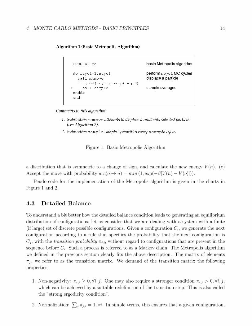
Figure 1: Basic Metropolis Algorithm
a distribution that is symmetric to a change of sign, and calculate the new energy V (n). (c)
Accept the move with probability acc(o→ n) = min (1, exp(−β[V (n)− V (o)])).
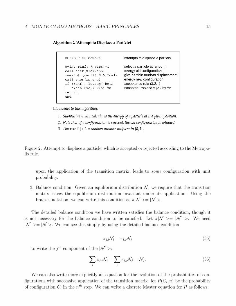
Peudo-code for the implementation of the Metropolis algorithm is given in the charts in
Figure 1 and 2.
4.3 Detailed Balance
To understand a bit better how the detailed balance condition leads to generating an equilibrium
distribution of configurations, let us consider that we are dealing with a system with a finite
(if large) set of discrete possible configurations. Given a configuration Ci, we generate the next
configuration according to a rule that specifies the probability that the next configuration is
Cj, with the transition probability πj,i, without regard to configurations that are present in the
sequence before Ci. Such a process is referred to as a Markov chain. The Metropolis algorithm
we defined in the previous section clearly fits the above description. The matrix of elements
πj,i we refer to as the transition matrix. We demand of the transition matrix the following
properties:
1. Non-negativity: πi,j ≥ 0,∀i, j. One may also require a stronger condition πi,j > 0,∀i, j,which can be achieved by a suitable redefinition of the transition step. This is also called
the ”strong ergodicity condition”.
2. Normalization:∑
j πj,i = 1,∀i. In simple terms, this ensures that a given configuration,
4 MONTE CARLO METHODS - BASIC PRINCIPLES 15
Figure 2: Attempt to displace a particle, which is accepted or rejected according to the Metropo-lis rule.
upon the application of the transition matrix, leads to some configuration with unit
probability.
3. Balance condition: Given an equilibrium distribution N , we require that the transition
matrix leaves the equilibrium distribution invariant under its application. Using the
bracket notation, we can write this condition as π|N >= |N >.
The detailed balance condition we have written satisfies the balance condition, though it
is not necessary for the balance condition to be satisfied. Let π|N >= |N ′>. We need
|N ′>= |N >. We can see this simply by using the detailed balance condition
πj,iNi = πi,jNj (35)
to write the jth component of the |N ′>:∑
i
πj,iNi =∑i
πi,jNj = Nj. (36)
We can also write more explicitly an equation for the evolution of the probabilities of con-
figurations with successive application of the transition matrix. let P (Ci, n) be the probability
of configuration Ci in the nth step. We can write a discrete Master equation for P as follows:
4 MONTE CARLO METHODS - BASIC PRINCIPLES 16
P (Ci, n+ 1) =∑j 6=i
πi,jP (Cj, n) + (1−∑j 6=i
πi,j)P (Ci, n) (37)
where the second term has been written using the normalization condition above. Rearranging,
we have
P (Ci, n+ 1) =∑j 6=i
[πi,jP (Cj, n)− πi,jP (Ci, n)] + P (Ci, n) (38)
If we demand that n→∞, P (Ci, n+1) = P (Ci, n) = Ni, then we see that the detailed balance
condition follows if we require that this be achieved by setting each term in the sum on the
right hand side to zero. This is therefore a sufficient but not necessary condition.
So far we have only shown that Ni is invariant under the application of π if π obeys detailed
balance. But we would like to be assured that an algorithm obeying detailed balance results
in a sequence of configurations that converges to the equilibrium distribution. This can be
demonstrated using the Perron’s theorem that states that every matrix with positive elements
has an eigen value that is real, positive and non-degenerate, which exceeds the modulus of
all other eigenvalues, with an eigen vector which has all positive elements. We can choose
this eigen value to be unity. The transition matrix satisfies the condition of the theorem, and
based on the discussion above, the corresponding eigen vector is the equilibrium distribution
|N >. Then, if we start with an arbitrary initial vector |P0 >, we can ask what happens upon
successive applications of the transition matrix. We have
πn|P0 >= |λ = 1 >< λ = 1|P0 > +∑λ 6=1
λn|λ >< λ|P0 > (39)
where λ are the eigen values of the matrix, and we have λ < 1. Hence, as n→∞,
πn|P0 >→ |λ = 1 >= |N > (40)
thus guaranteeing convergence to the equilibrium distribution.
4.4 Random Numbers
In implementing a procedure such as the one above, you will note that you need to generate
“random numbers”. There are many methods for generating and testing the goodness of random
number sequences, discussed in various books, e. g., “Numerical Recipes: The Art of Scientific
Computing” by W. H. Press et al (Cambridge University Press). We will assume that such
generators are available for use.
A common generator is the linear congruential pseudo random number generator,
Ri+1 = [a×Ri + b](mod m)
which, for a good choice of a, b and m, generates numbers that appear to satisfy conditions
that we expect for random numbers, in that they are uniformly distributed over the interval
4 MONTE CARLO METHODS - BASIC PRINCIPLES 17
[0,m] and have no obvious sequence. Dividing by m generates numbers between 0 and 1.
The ”pseudo-random” numbers generated however clearly have a repeat cycle which is at most
m long. Further, it has been shown (”Random numbers fall mainly in the planes” by G
Marsaglia, PNAS 61, 25 (1968)) that if one uses n-tuples (R1, R2 . . . Rn), (R2, R3 . . . Rn+1) as
coordinates for points in an n dimensional space, they lie on planes, and are therefore strongly
correlated. A once widely used IBM subroutine called RANDU, with a = 65539, c = 0,m = 231
apparently produced very bad sets of random numbers. Hence, random number generators must
be carefully tested before they are used. Possible good choices have been explored, and one
recommended set is a = 16805, b = 0,m = 232 − 1. Additional details are found in “Numerical
Recipes” and references therein.
Suppose we want to generate a random number sequence distributed not uniformly between
0 and 1 but, say, according to an exponential distribution. The method used is to convert
the uniform random numbers x to the desired distribution. Consider function y(x). Given the
probability distribution of x, p(x), we have the relation
p(x)dx = p(y)dy
or
p(y) = p(x)|dxdy|
If we choose
y(x) = − log(x)
Then by the application of the above result, since we have p(x) = 1,
p(y) = exp(−y).
As an introduction to the Monte Carlo approach to computations, and to explore issues
relevant to such computations, we consider the following exercise:
4 MONTE CARLO METHODS - BASIC PRINCIPLES 18
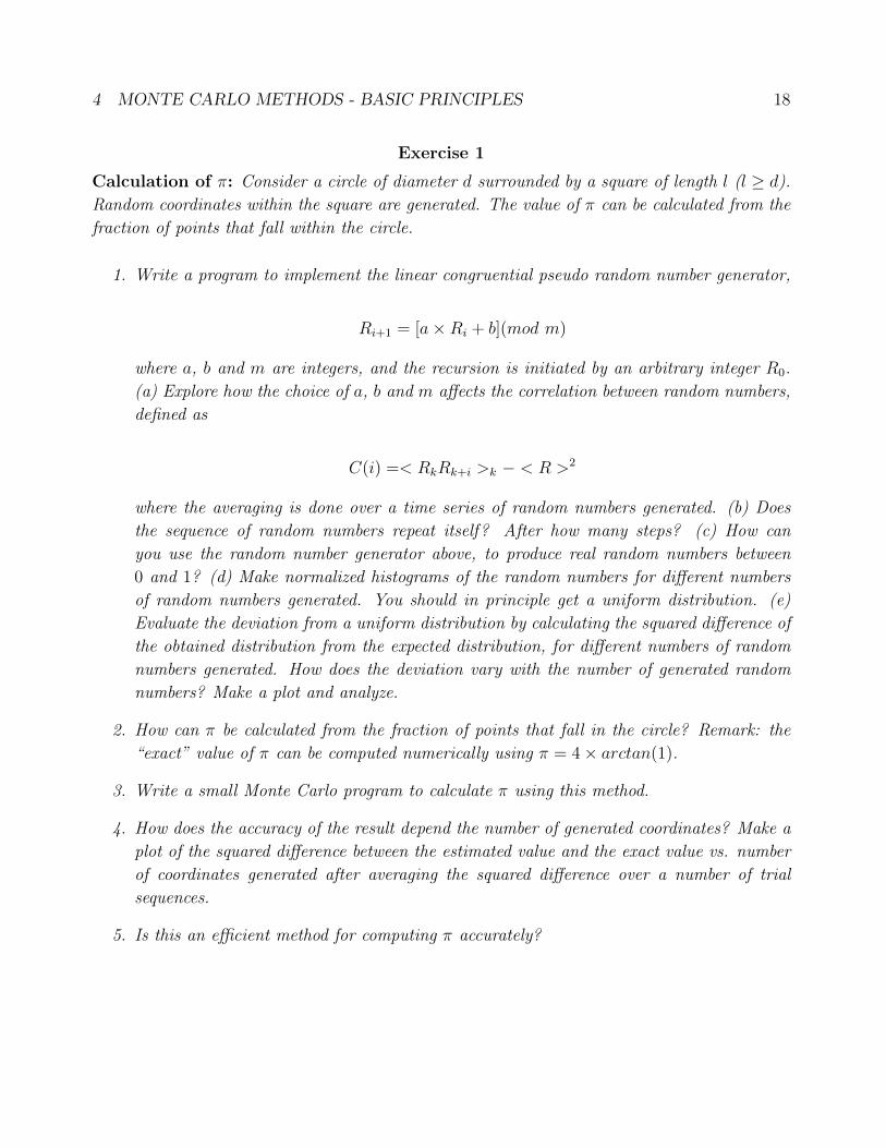
Exercise 1
Calculation of π: Consider a circle of diameter d surrounded by a square of length l (l ≥ d).
Random coordinates within the square are generated. The value of π can be calculated from the
fraction of points that fall within the circle.
1. Write a program to implement the linear congruential pseudo random number generator,
Ri+1 = [a×Ri + b](mod m)
where a, b and m are integers, and the recursion is initiated by an arbitrary integer R0.
(a) Explore how the choice of a, b and m affects the correlation between random numbers,
defined as
C(i) =< RkRk+i >k − < R >2
where the averaging is done over a time series of random numbers generated. (b) Does
the sequence of random numbers repeat itself? After how many steps? (c) How can
you use the random number generator above, to produce real random numbers between
0 and 1? (d) Make normalized histograms of the random numbers for different numbers
of random numbers generated. You should in principle get a uniform distribution. (e)
Evaluate the deviation from a uniform distribution by calculating the squared difference of
the obtained distribution from the expected distribution, for different numbers of random
numbers generated. How does the deviation vary with the number of generated random
numbers? Make a plot and analyze.
2. How can π be calculated from the fraction of points that fall in the circle? Remark: the
“exact” value of π can be computed numerically using π = 4× arctan(1).
3. Write a small Monte Carlo program to calculate π using this method.
4. How does the accuracy of the result depend the number of generated coordinates? Make a
plot of the squared difference between the estimated value and the exact value vs. number
of coordinates generated after averaging the squared difference over a number of trial
sequences.
5. Is this an efficient method for computing π accurately?

5 MONTE CARLO SIMULATION OF LATTICE AND OFF-LATTICE SYSTEMS 19
5 Monte Carlo simulation of lattice and off-lattice sys-
tems
5.1 Monte Carlo simulations: Examples
In this section we will discuss the technical details that must be addressed in order to implement
a Monte Carlo simulation. We consider two examples. The first is a system of particles which
interact with each other with the Lennard-Jones interaction potential. The second is an example
of a lattice system, the Ising model.
The Lennard-Jones system
The Lennard-Jones interaction potential given by
U(r) = 4ε
[(σr
)12
−(σr
)6].
The Lennard-Jones interaction represents the interactions that would exist between neutral
atoms, with a short range repulsive interaction arising from the overlapping of electron orbitals,
and a longer range attractive interaction, arising from dispersion or van der Waals forces. This
potential can be a reasonable for the interaction between noble gas atoms, such as Argon.
The potential is described by two parameters, the size of the atoms, σ, and the strength of
interaction, ε. In addition, the specification of a given atom would also require the mass
m. The values of these parameters for Argon are σ = 3.405 × 10⁻¹⁰m, ε/kB = 119.8K,
m = 0.03994kg/mol. Note that the scale of energy, ε has been specified in terms of temperature.
This, apart from being legitimate, is also useful. When one is interested in the dependence
of the properties of a material on temperature, the main role played by the energy scale of
interaction is to set the temperature scale that is relevant. In other words, if one were to scale
the temperatures for different substances by their interaction energy scales, one might expect
the same physical phenomena to occur at the same scaled temperatures, which is related to the
law of corresponding states. Thus, it is natural that instead of working with the size, energy
scale and mass of specific materials, it may be more instructive to use reduced units, where
energies are expressed, instead of in, e. g., S. I. units, in units of the energy scale ε. Thus, the
energy in reduced units will be related to the energy in S. I. units by U∗ = Uε−1. Similarly, the
time in reduced units will be expressed in units of σ√
(m/ε) (though we won’t worry about time
in Monte Carlo simulations), temperature in units of ε/kB, pressure in units of εσ−3, density
in units of σ−3. Thus, T ∗ = kBT/ε, P∗ = Pσ3ε−1, ρ∗ = ρσ3 express the relation between
reduced temperature, pressure and density to their usual counterparts. Most simulation codes
for potentials such as the Lennard-Jones potential are written in reduced units, and conversion
to S. I. units for specific materials is made only at the stage of expressing the final results. Such
a procedure also has the advantage of eliminating a certain amount of unnecessary floating point
arithmetic in our computations.
Boundary Conditions: In computer simulations, we are able to do a few hundred, up to

5 MONTE CARLO SIMULATION OF LATTICE AND OFF-LATTICE SYSTEMS 20
a few million particle simulations, which are still very far from the thermodynamically large
numbers we have discussed earlier. Nevertheless, we wish to extract useful information from our
simulations about the behavior of bulk systems with large (of the order of Avogadro’s number)
numbers of interacting particles. One crucial feature that affects how closely our simulated
system may or may not resemble bulk systems is the boundary conditions we employ. Suppose
we use open boundary conditions in simulating a crystal in the form of a cube. As one can
easily verify, nearly 50 % of all the atoms will reside on the boundary, and thus have a local
environment that is very different than what an atom in a bulk system would experience. A
solution to this problem is the use of periodic boundary conditions, as illustrated in Figures
3. The simulation volume or cell in which we have particles is treated as the unit cell of an
infinite lattice of cells that repeat periodically in space. Thus a given particle in the primary
cell interacts not only with other particles in that cell, but also with all the periodic images. On
the face of it, this appears to be a foolish thing to do, as we now have to worry about doing a
large number of computations, which we presumably were trying to avoid by doing a simulation
with a small number of particles. However, in practice, the need for such large computations is
avoided. In the simpler case, one has a system of particles with short ranged interactions. In
this case, we only have to consider images within some short range. In the more complicated
case when the interactions are long ranged, as in the important case of Coulombic interactions,
as we will see later, other methods are employed to avoid the need to consider interactions with
all the image particles.
Figure 3: Schematic representation of periodic boundary conditions.
Truncation of the potential: Somewhat associated with the issue of periodic boundary
conditions is the procedure of truncation of the interaction potential. Consider the Lennard-
Jones potential. Even though it is short ranged in the sense that it becomes rapidly negligible
at large r, it is finite at all r. One normally calculates interactions only up to a cutoff distance
rc, either accounting for the interactions at larger distances in the quantities calculated, or
5 MONTE CARLO SIMULATION OF LATTICE AND OFF-LATTICE SYSTEMS 21
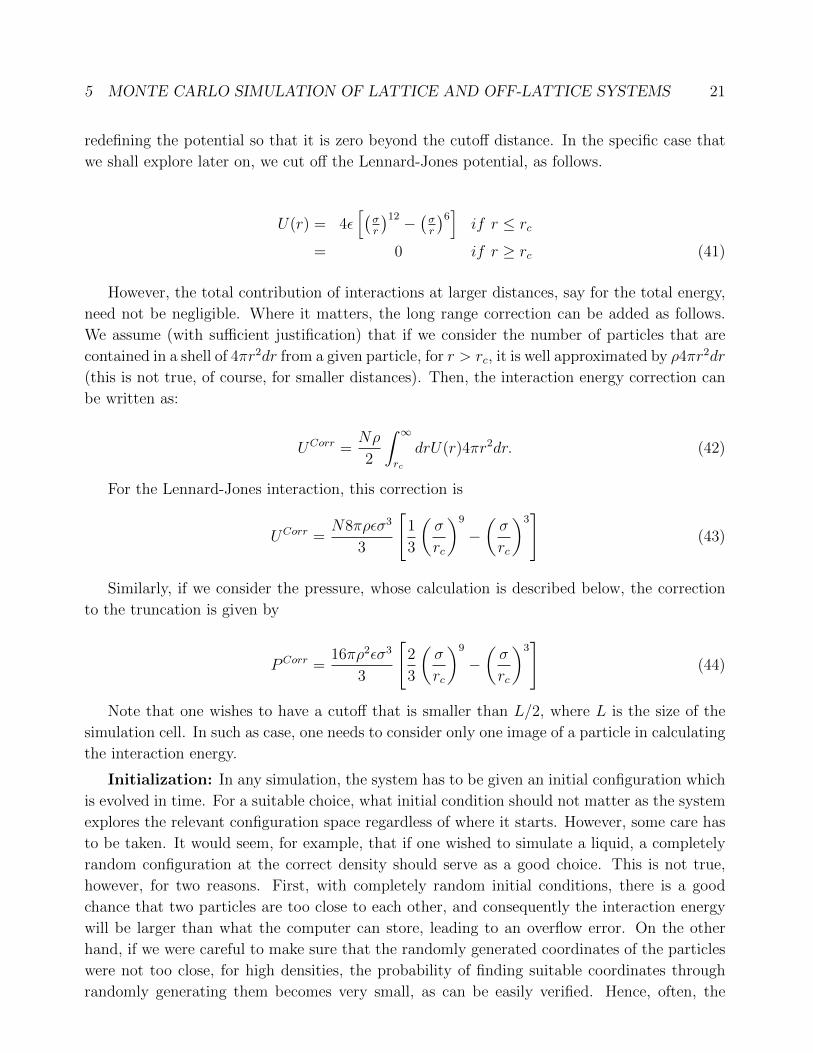
redefining the potential so that it is zero beyond the cutoff distance. In the specific case that
we shall explore later on, we cut off the Lennard-Jones potential, as follows.
U(r) = 4ε[(
σr
)12 −(σr
)6]
if r ≤ rc
= 0 if r ≥ rc (41)
However, the total contribution of interactions at larger distances, say for the total energy,
need not be negligible. Where it matters, the long range correction can be added as follows.
We assume (with sufficient justification) that if we consider the number of particles that are
contained in a shell of 4πr2dr from a given particle, for r > rc, it is well approximated by ρ4πr2dr
(this is not true, of course, for smaller distances). Then, the interaction energy correction can
be written as:
UCorr =Nρ
2
∫ ∞rc
drU(r)4πr2dr. (42)
For the Lennard-Jones interaction, this correction is
UCorr =N8πρεσ3
3
[1
3
(σ
rc
)9
−(σ
rc
)3]
(43)
Similarly, if we consider the pressure, whose calculation is described below, the correction
to the truncation is given by
PCorr =16πρ2εσ3
3
[2
3
(σ
rc
)9
−(σ
rc
)3]
(44)
Note that one wishes to have a cutoff that is smaller than L/2, where L is the size of the
simulation cell. In such as case, one needs to consider only one image of a particle in calculating
the interaction energy.
Initialization: In any simulation, the system has to be given an initial configuration which
is evolved in time. For a suitable choice, what initial condition should not matter as the system
explores the relevant configuration space regardless of where it starts. However, some care has
to be taken. It would seem, for example, that if one wished to simulate a liquid, a completely
random configuration at the correct density should serve as a good choice. This is not true,
however, for two reasons. First, with completely random initial conditions, there is a good
chance that two particles are too close to each other, and consequently the interaction energy
will be larger than what the computer can store, leading to an overflow error. On the other
hand, if we were careful to make sure that the randomly generated coordinates of the particles
were not too close, for high densities, the probability of finding suitable coordinates through
randomly generating them becomes very small, as can be easily verified. Hence, often, the
5 MONTE CARLO SIMULATION OF LATTICE AND OFF-LATTICE SYSTEMS 22
initial condition of choice is a crystalline lattice, but one must ensure, if one wishes to simulate
a liquid, that the crystal lattice melts before one begins to calculate averages of quantities of
interest. This is normally done by a short simulation at the outset at a very high temperature.
Trial Moves: In order to generate new configurations, we create trail coordinates for
particles, and calculate the energy for the new coordinates in order to execute a Metropolis step.
The first question that may arise is whether it is better to attempt changing the coordinates
of one particle at a time or all particles at the same time. Considering the probability of
acceptance, we see that for a successful move, the net change in energy should be comparable
to kBT , so that when the energy increases, exp(−β∆E) is not too small. If one imagines that
all the particles experience a roughly harmonic potential at a given instant, then the ratio of
kBT to the average curvature gives an estimate of the squared distance (by a single particle or
all particles added together) should move. At this level, we can make either choice. However,
for the same squared displacement, in the case we move all the particles, the computational
effort of calculating the new energy is N times larger. If the squared displacement is a good
measure of how well the simulation performs (which is the case, as it is a measure of how well
the configuration space is explored), then it is clearly better to update single particles at a
time. Hence, we consider updates of single particle coordinates, of the form:
x′= x+ ∆ (rand− 1
2) (45)
where rand is a random number, and the subtraction of 1/2 ensures statistically the symmetry
of the trial moves. The next question is how big the step size, ∆, should be. If ∆ is too
small, all moves are accepted as the energy change will be very small, but the sum of squared
displacements will be small. At the other extreme, if the step sizes are very large, very few
moves are accepted, and here also, the sum of squared displacements will be very small. There
will be a range in between where the acceptance probability is considerable, and the step size
is also not small, where one expects to get the most efficient exploration of configuration space.
As we do not know a priori what the optimum step size is, the procedure that is followed
is to adjust it to achieve a given percentage of accepted moves, usually 50 %, though careful
studies suggest that a smaller acceptance probability, such as 20 %, might lead to more efficient
simulations.
Calculation of the potential and other quantities: Since the calculation of energies
and forces is at the heart of a Monte Carlo (and Molecular Dynamics) simulation, it is important
that it is done efficiently, minimizing the number of operations needed. A scheme of how this
may be done (for a slightly different potential than what we propose to use, and calculating
both energy and forces) is shown in Figure 4.
In addition to the energy, a thermodynamic quantity that one typically wishes to calculate
is the pressure. The pressure is calculated in simulations using
P = kBTρ+1
V< W >, (46)

5 MONTE CARLO SIMULATION OF LATTICE AND OFF-LATTICE SYSTEMS 23
Figure 4: Calculation of energy and forces.
where W , the virial, is given by
W =1
3
∑i
∑j>i
rij.fij =1
3
∑i
∑j>i
w(rij) (47)
where for pair-wise interactions, we have w(r) = −r dv(r)dr
. For the Lennard-Jones potential,
w(r) = 48ε
[(σr
)12
− 1
2
(σr
)6]. (48)
The calculation of the virial therefore can be easily incorporated into the routine that
calculates the forces.
Neighbor Lists: Neighbor lists are used to keep track of particles within a cutoff distance
rv of each particle (where rv is greater by a small amount than the interaction cutoff rc) so
that the calculation of particle distances at each integration step will be of order N rather
than N2. In order to ensure that all the neighbors within the interaction distance cutoff are
accounted for, one must decide when to update the neighbor list. For this one keeps track of how
much each particle has moved from the last time the neighbor list was calculated, ∆ri. When
the maximum displacement |∆maxi | ≥ |rv − rc|/2 (which is the worst case when two particles,
5 MONTE CARLO SIMULATION OF LATTICE AND OFF-LATTICE SYSTEMS 24
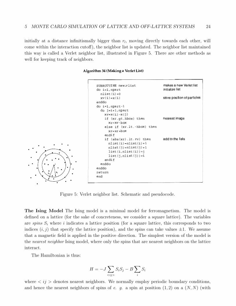
initially at a distance infinitismally bigger than rl, moving directly towards each other, will
come within the interaction cutoff), the neighbor list is updated. The neighbor list maintained
this way is called a Verlet neighbor list, illustrated in Figure 5. There are other methods as
well for keeping track of neighbors.
Figure 5: Verlet neighbor list. Schematic and pseudocode.
The Ising Model The Ising model is a minimal model for ferromagnetism. The model is
defined on a lattice (for the sake of concreteness, we consider a square lattice). The variables
are spins Si where i indicates a lattice position (for a square lattice, this corresponds to two
indices (i, j) that specify the lattice position), and the spins can take values ±1. We assume
that a magnetic field is applied in the positive direction. The simplest version of the model is
the nearest neighbor Ising model, where only the spins that are nearest neighbors on the lattice
interact.
The Hamiltonian is thus:
H = −J∑<ij>
SiSj −B∑i
Si
where < ij > denotes nearest neighbors. We normally employ periodic boundary conditions,
and hence the nearest neighbors of spins of e. g. a spin at position (1, 2) on a (N,N) (with
5 MONTE CARLO SIMULATION OF LATTICE AND OFF-LATTICE SYSTEMS 25
indices running from 1 to N) lattice are at (N, 2), (2, 2), (1, 1), (1, 3).
For applying the Metropolis algorithm, we must specify the trial moves. In the case of the
Ising model, the trial moves are flips of the spin. Thus, is we consider a configuration where
Si = 1 in the initial configuration, the trial state is Striali = −1.
Exercise 2
i: Generate in a volume L × L × L, L = 4, a random configuration of N = 100 spheres of
radium r, which may overlap. Vary r between values r = 0.01 to r = 2. Calculate the
probability that a randomly picked point in space lies outside all of the spheres by perform-
ing a Monte Carlo sampling of the volume (determine how many trials are sufficient to
generate good results. Can you determine the form of the probability? Can you derive it?
Make random displacements of the spheres by a step size L/10 along each axis. Some of
the resulting coordinates may lie outside the volume. Apply periodic boundary conditions
to determine the coordinate of an image that lies within the ”primary cell” (coordinates
between 0 and L). Iterate the process for each configuration 100 times. Repeat the exercise
of finding the probability that a randomly picked point lies outside the spheres. Does it
change?
ii: Consider the Ising model with J = 0, in a magnetic field B = 1. This corresponds to
a paramagnet. Varying the temperature from T = 4 to T = 0.1, plot the magnetization
M = 1N
∑i Si. Compare with the exact result.
Exercise 3
Using the Monte Carlo code you have developed for Assignment 1 for the shifted force
Lennard-Jones potential, do a series of short simulations (1000 MCS) with 6 - 8 different
system sizes starting with N = 108, going up to as large a system as you can in less than an
hour of single CPU time, with and without the use of neighbor lists, and plot the average time
per MCS as a function of system size.

5 MONTE CARLO SIMULATION OF LATTICE AND OFF-LATTICE SYSTEMS 26
5.2 Monte Carlo simulations in various ensembles
So far, we have discussed Monte Carlo simulations in the canonical (N,V,T) ensemble. In
principle, for the calculation of average properties such as, say the pressure of a liquid, it is
adequate to work with any given ensemble, as the calculation of average quantities in different
ensembles is equivalent. However, there are many situations (such as simulations in the presence
of a liquid-gas phase transition, in the vicinity of the transition line) where it is desirable to
have flexibility in the ensemble one does the simulation in. In the example mentioned, it
would, e. g. be preferable to do (N,P, T ) simulations so that one always simulates a single
phase system (as opposed to (N,V,T) where one may simulate a heterogeneous system if one
chooses density and temperatures in the coexistence region). Further, it will be possible to to
define simulation ensembles that do not correspond to the conventional ensembles, which allow
efficient calculation of phase boundaries, etc. Here we describe the methods for performing
Monte Carlo simulations in a few different ensembles.
Monte Carlo in the (N,P, T ) ensemble:
We derive the update equations for the NPT ensemble by considering the system we are
interested in simulating as a subsystem of a larger system, as shown in the schematic in Figure
8. Here and in the next section, we treat the particles as identical particles, but assume that
while they are in the sub-volume of interest (called the system), they interact with each other
with the desired interaction potential, while in the “bath” they behave like an ideal gas (i. e.
they do not interact with each other. For the NPT ensemble, this is perfectly simple, but in
the grand canonical case we deal with in the next section, even though we exchange particles
between the bath and the system, we maintain this assumption). For an N particle system, we
will write the partition function in terms of scaled coordinates, as
Figure 6: Schematic representation of the extended system treated in developing the NPTMonte Carlo algorithm.

5 MONTE CARLO SIMULATION OF LATTICE AND OFF-LATTICE SYSTEMS 27
Q(N, V, T ) =1
Λ3NN !
∫ L
0
drN exp[−βU(rN)] (49)
=V 3N
Λ3NN !
∫ 1
0
dsN exp[−βU(sN ;L)].
Now consider that we have a piston that separates the system and the bath, with total
volume V0, total number of particles M , and the system has volume V and number of particles
N . V can change, but first we consider writing the partition with the system volume fixed.
The total partition function is a product of the system and bath partition functions, and is
given by
Q(N,M, V, V0, T ) =V N(V0 − V )(M−N)
Λ3MN !(M −N)!
∫dsM−N
∫dsN exp[−βU(sN ;L)]. (50)
The integral over sM−N will be unity. Now if we assume that the system volume can vary,
the probability that it takes a particular value V is given by
N (V ) =V N(V0 − V )(M−N)
∫dsN exp[−βU(sN ;L)]∫
dV ′V ′N(V0 − V ′)(M−N)∫dsN exp[−βU(sN ;L′)]
. (51)
We consider now the limit when the size of the bath tends to infinity while keeping the density
fixed: i. e. V0 → ∞,M → ∞, (M − N)/V0 → ρ. In this limit, (V0 − V )(M−N) = V(M−N)
0 (1 −(V/V0))(M−N) → V
(M−N)0 exp(−ρV ). However, we can use the ideal gas equation of state to
write ρ = βP . We can therefore write
NN,P,T (V ) =V N exp(−βPV )
∫dsN exp[−βU(sN ;L)]∫
dV ′V ′N exp(−βPV ′)∫dsN exp[−βU(sN ;L′)]
. (52)
The corresponding partition function is written (with βP included for dimensional reasons)
as:
Q(N,P, T ) =βP
Λ3NN !
∫dV V N exp(−βPV )
∫dsN exp[−βU(sN ;L)]. (53)
If we now consider volume change attempts of the form V′= V +∆V where ∆V is uniformly
distributed in an interval [−∆Vmax,∆Vmax], the acceptance probability that will result in the
detailed balance condition is:
acc(o→ n) = min(
1, exp(−β[U(sN , V′)− U(sN , V ) + P (V
′ − V )−Nβ−1 ln(V′/V )]
). (54)
Instead of making trial changes in V , one can consider making changes in lnV . For this case,
we can write the partition function as
Q(N,P, T ) =βP
Λ3NN !
∫d lnV V N+1 exp(−βPV )
∫dsN exp[−βU(sN ;L)]. (55)
5 MONTE CARLO SIMULATION OF LATTICE AND OFF-LATTICE SYSTEMS 28
The corresponding acceptance probability will be
acc(o→ n) = min(
1, exp(−β[U(sN , V′)− U(sN , V ) + P (V
′ − V )− (N + 1)β−1 ln(V′/V )]
).
(56)
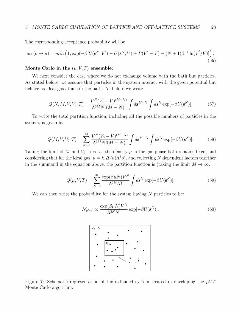
Monte Carlo in the (µ, V, T ) ensemble:
We next consider the case where we do not exchange volume with the bath but particles.
As stated before, we assume that particles in the system interact with the given potential but
behave as ideal gas atoms in the bath. As before we write
Q(N,M, V, V0, T ) =V N(V0 − V )(M−N)
Λ3MN !(M −N)!
∫dsM−N
∫dsN exp[−βU(sN)]. (57)
To write the total partition function, including all the possible numbers of particles in the
system, is given by:
Q(M,V, V0, T ) =M∑N=0
V N(V0 − V )(M−N)
Λ3MN !(M −N)!
∫dsM−N
∫dsN exp[−βU(sN)]. (58)
Taking the limit of M and V0 →∞ as the density ρ in the gas phase bath remains fixed, and
considering that for the ideal gas, µ = kBT ln(Λ3ρ), and collecting N dependent factors together
in the summand in the equation above, the partition function is (taking the limit M →∞:
Q(µ, V, T ) =∞∑N=0
exp(βµN)V N
Λ3NN !
∫dsN exp[−βU(sN)]. (59)
We can then write the probability for the system having N particles to be:
NµV T ∝exp(βµN)V N
Λ3NN !exp[−βU(sN)]. (60)
Figure 7: Schematic representation of the extended system treated in developing the µV TMonte Carlo algorithm.
5 MONTE CARLO SIMULATION OF LATTICE AND OFF-LATTICE SYSTEMS 29
Based on this probability, we can write the acceptance probabilities for a particle to be
randomly inserted in the system, or for a randomly selected particle to be removed, as:
acc(N → N + 1) = min
(1,
V
Λ3(N + 1)exp(β[µ− U(N + 1) + U(N)])
). (61)
and
acc(N + 1→ N) = min
(1,
Λ3N
Vexp(−β[µ+ U(N − 1)− U(N)])
). (62)
Note that the Λ3NV
can be written in terms of the ideal gas chemical potential so that this
term (and the corresponding term in the previous expression) can be combined with µ, and
result in expressions that require only the excess (total minus the ideal gas) chemical potential
needs to be specified.
6 MOLECULAR DYNAMICS SIMULATIONS - BASIC PRINCIPLES 30
6 Molecular dynamics simulations - basic principles
The other major technique used in simulating equilibrium properties of many body systems is
the molecular dynamics method. Unlike the Monte Carlo method, for which we needed to argue
that the procedure will generate an equilibrium ensemble of states, the molecular dynamics
method does not need much justification as far as validity is concerned. In developing the ideas
of statistical mechanics, we started out with the microscopic dynamics as determining the time
evolution of a many body system, and tried to find an alternate, more tractable formulation
for calculating desirable macroscopic properties. In using molecular dynamics, we go back, in
some sense, to plain mechanics. We will simply integrate the equations of motion of a many
body system numerically in order to obtain its trajectory in phase space. However, we employ
the language of statistical mechanics in analyzing the trajectory to extract useful information.
In addition to equilibrium thermodynamic properties, the use of molecular dynamics gives us
access to studying dynamical properties as well. We will discuss a few of such properties in due
course.
The structure of a molecular dynamics, like a Monte Carlo simulation, involves initialization,
generating a series of configurations, and sampling these configurations to evaluate averages of
interest. The initialization of positions is done in the same way as in Monte Carlo, in MD,
one has to initialize velocities as well. Typically, the velocities are initialized by specifying
a temperature, although at present we discuss only the case of constant energy simulations.
With a target temperature, in principle one can generate a Maxwell distribution of velocities,
but this is not really necessary. The Maxwell distribution is generated by the dynamics of the
system regardless of the initial distribution. It is sufficient to generate individual components
of the velocity symmetrically around zero. After the velocities are generated, the center of mass
velocity is calculated and set to zero. This is done because the uniform motion of our system
is of no interest to us, but more importantly, the calculation of the average temperature using
the velocities will be in error if a center of mass velocity is present. We use the equipartition
theorem,m
2
∑i
v2i =
3
2NkBT (63)
to obtain the temperature from the velocities. During initialization, this relation is used to
determine the magnitude of the initial velocities.
While in Monte Carlo, the series of configurations is generated by a stochastic process em-
ploying the Metropolis algorithm, and does not contain any explicit notion of time, in molecular
dynamics we generate a time series along a trajectory of the system. Thus the procedure for
generating the new configurations is to evaluate forces acting on the particles and integrating
the equations of motion. The calculation of the forces (for the example of the truncated and
shifted Lennard-Jones potential) is illustrated in Figure 4. This is the most time consuming
part of a molecular dynamics simulation, and methods to reduce the computational load, such
as the Verlet neighbor list already discussed (shown in Figure 5) are routinely employed.

6 MOLECULAR DYNAMICS SIMULATIONS - BASIC PRINCIPLES 31
The integration of the equations of motion are done by a variety of algorithms, and we start
by one of the most commonly used, the Verlet algorithm. We can write the Taylor series of the
coordinate of a particle, around time t, as
r(t+ ∆t) = r(t) + v(t)∆t+f(t)
2m∆t2 +
∆t3
3!
...r +O(∆t4). (64)
Considering the expansion for a negative time increment and taking the difference, such
that the odd terms drop out, gives
r(t+ ∆t) + r(t−∆t) = 2r(t) +f(t)
m∆t2 +O(∆t4), (65)
or
r(t+ ∆t) = 2r(t)− r(t−∆t) +f(t)
m∆t2. (66)
This is the Verlet algorithm, which is accurate to ∆t4, and it does not use the velocities in
the update but instead the position at two times. One can of course obtain the velocities by a
difference of positions,
v(t) =r(t+ ∆t)− r(t−∆t)
2∆t+O(∆t2). (67)
The accuracy of the velocities is up to second order only, which will affect, e. g., the values
of total energy. However, this is not an indication of the order of accuracy of the integrator
itself. Finally, the Verlet algorithm is time reversible as can be seen explicitly in the update
equation.
Some other robust algorithms can be shown to be equivalent to the Verlet algorithm, such
as the Leap Frog algorithm:
r(t+ ∆t) = r(t) + ∆t v(t+ ∆t/2)
v(t+ ∆t/2) = v(t−∆t/2) + ∆tf(t)
m. (68)
The velocities, in the Leap Frog algorithm are defined for the mid-step. The velocity Verlet
algorithm, which also generates the same trajectories as Verlet and Leap Frog, uses equal time
velocities and positions, and is given by
r(t+ ∆t) = r(t) + ∆t v(t) + ∆t2f(t)
2m.
6 MOLECULAR DYNAMICS SIMULATIONS - BASIC PRINCIPLES 32
v(t+ ∆t) = v(t) + ∆tf(t) + f(t+ ∆t)
2m. (69)
The velocities therefore have to be updated twice if the forces are stored for only one time,
with the forces before and after the position update.
How do we compare algorithms to decide which may be better than another? An obvious
criterion might seem to be to compare the numerically integrated trajectory with known exact
results in some cases, or to compare with more and more precise trajectories that we can
always obtain by choosing smaller time steps. This, however, turns out not to be a good
criterion for a fundamental reason. Trajectories of many body interacting particles display
Lyapunov instability, which causes nearby trajectories in phase space to diverge from each other
exponentially. That means that even if there was a very minute discrepancy in our estimate of
coordinates compared to the “true” trajectory, this will grow exponentially in time and become
significant very quickly. Thus it seems hopeless to think of faithfully generating trajectories of
such systems. However, for our purposes, we don’t need the exact trajectories really, as our
purpose is to calculate statistical properties along the trajectory. What we need is that the
trajectories belong to the intended phase space and sample it correctly. As a concrete criterion,
as we perform constant energy simulations, even if the trajectories are unstable, if they remain
in the sub-space that corresponds to the chosen energy, this will be good enough for us. Thus,
the criteria to evaluate the integrators will be time reversibility, energy conservation, lack of
energy drift and related notions. From these points of view, the Verlet algorithm proves to
be robust, as can be seen from a theoretical analysis sketched below, which provides a general
scheme for developing integration schemes.
For a general function of positions and moment, we can write the time evolution as
f(r,p) = r∂f
∂r+ p
∂f
∂p≡ iLf (70)
where r and p stand for the coordinates and momenta of all the particles in the system, and
the Liouville operator is defined by
iL = r∂
∂r+ p
∂
∂p. (71)
We can formally integrate the equation for f to write
f(r(t),p(t)) = exp(iLt)f(r,p) (72)
This, however is not very useful. To develop concrete algorithms, we consider first the
position and momentum parts of the Liouville operator separately, as
iLr = r∂
∂r; iLpp
∂
∂p, (73)

6 MOLECULAR DYNAMICS SIMULATIONS - BASIC PRINCIPLES 33
and note that each of them generates a shift in coordinates and momenta respectively. Thus,
considering only iLr, we can write
f(t) = f(0) + iLrtf(0) +(iLrt)
2
2f(0) + . . . (74)
=∞∑n=0
(r(0)t)n
n!
∂n
∂rnf(0)
= f(p(0), (r(0) + r(0)t).
In applying the two components of the operator together, however, we are faced with the fact
that the two operators do not commute and therefore we cannot write exp(iLt) = exp(iLrt)×exp(iLpt). However, we have the Trotter identity,
exp(A+B) = limp→∞
[exp(
A
2p) exp(
B
p) exp(
A
2p)
]p. (75)
For finite p, we have
exp(A+B) =
[exp(
A
2p) exp(
B
p) exp(
A
2p)
]pexp(O(1/p2)). (76)
We consider the case A/p = iLpt/p and B/p = iLrt/p and ∆t = t/p. Thus, with p = 1, one
step in this corresponds to
exp(iLp∆t/2) exp(iLr∆t) exp(iLp∆t/2). (77)
Let us consider this step by step.
exp(iLp∆t/2)f(p, r) = f(p +∆t
2p, r). (78)
Next,
exp(iLr∆t)f(p +∆t
2p, r) = f(p +
∆t
2p, r + ∆tr(∆t/2)) (79)
Finally,
exp(iLp∆t/2)f(p +∆t
2p, r + ∆tr(∆t/2)) = f(p +
∆t
2p +
∆t
2p(∆t), r + ∆tr(∆t/2)). (80)
Considering now how the momenta and positions have been transformed, we have, using
p = F,
p(0) → p +∆t
2F(0) +
∆t
2F(∆t) (81)
r(0) → r + ∆tr(∆t
2) (82)
= r + ∆tr(0) +∆t2
2mF(0). (83)

6 MOLECULAR DYNAMICS SIMULATIONS - BASIC PRINCIPLES 34
These we identify as the update rules for the velocity Verlet algorithm. Higher order algo-
rithms can be derived using the above procedure, but we see that the Verlet algorithm arises
naturally out of this systematic analysis.
To get a feeling for the reliability and stability of integration schemes we apply two of them
to a simple harmonic oscillator, as outlined below.
Exercise 4: (simple harmonic oscillator)
Consider a simple harmonic oscillator,
d2x
dt2= − k
mx
Use units for which ω2 ≡ k/m = 1. Express the above equation as two first order equations
for x and v = dxdt
. Use x(0) = 0 and v(0) = 1. Integrate using the Euler and velocity verlet
algorithms, with different step sizes, for ∆t = 0.00001, 0.0001, 0.001, 0.01, 0.1, 0.2, 0.5. The
Euler scheme for an equation of form dydt
= f(t, y(t)) is yn+1 = yn + ∆tf(tn, yn). For each case,
monitor the deviation from the known exact solution vs. time. Identify the time beyond which
the solution deviates from the exact solution by amount ∆x = 0.05 (at which time we declare
the integration unreliable) and plot it against the time step. Identify the time step beyond which
the algorithm becomes unreliable before one period is completed.
6.1 Special Cases: Long range forces, Event driven MD, Molecularsystems
So far, we have discussed the evaluation of forces and integration of the equation of motion
keeping in mind a short range pair-wise atomic potential like the Lennard-Jones potential.
There are three classes of special cases we discuss here which need different treatment. The first
is the frequent use of model potentials with piece-wise constant. The simplest of these potentials
is the hard core potential. The second class is molecular systems, which are often modeled as
rigid bodies rather than treat e. g. bond vibrations which are fast and hence expensive, and
also not needed in most applications. Here, the problem is to work with constraints. The
last special case is the treatment of long range interactions. The methods of truncation and
correction we have discussed so far will not be effect when we have, e. g. Coulomb interactions.
Hence we need special methods to treat such cases.
Event driven molecular dynamics: hard spheres, square well potentials etc
Unlike continuous potentials discussed so far, systems where particles are treated as “hard”
particles (the interaction potential is zero beyond the diameter of the particles, but infinite for
separations less than the diameter of the particles) the forces acting on the particles are either
zero or act instantaneously at the moment of collision to impart an instantaneous change in the
velocities (impulse). For these, the updating of the dynamics is better handled by keeping track
of when collisions occur, and updating the positions of particles at constant velocity between
6 MOLECULAR DYNAMICS SIMULATIONS - BASIC PRINCIPLES 35
collisions. This is the idea of event driven dynamics which also finds application in simulating
potentials such as the square well potential which has a similar feature of instantaneous change
in velocities.
The dynamics is implemented in the following steps (illustrated for hard spheres of uniform
size):
1. Locate the next collision for each pair of particles: Given positions and velocities at some
time, the time to the collision between particles i and j, tit is given by the condition:
|rij + vijtij| = σ (84)
where rij and vij are relative positions and velocities and σ is the size of the hard spheres.
Defining bij = rij.vij
v2ijt
2ij + 2bijtij + r2
ij − σ2 = 0 (85)
We have the following cases:
i. If bij > 0 the particles are moving away.
ii. If b2ij − v2
ij(r2ij − σ2) < 0 the roots of the above equation are complex and a collision
will not take place.
iii. Else, the smaller of the solutions to the above equation gives the collision time to be
tij =−bij − (b2
ij − v2ij(r
2ij − σ2))1/2
v2ij
(86)
2. Find the pair of particles that will collide first by finding i, j for which tij is smallest
(≡ tminij ).
3. Propagate all particles by a time interval equal to tminij with constant velocity.
4. For the colliding particles, invert the velocities along the line of collision:
vi = voi + δv (87)
vj = voj − δv (88)
where
δv = −bijσ2
rij (89)

6 MOLECULAR DYNAMICS SIMULATIONS - BASIC PRINCIPLES 36
5. Return to step 1. Repeat. Keep track of time elapsed.
Molecular Systems:
When one considers molecular systems (the example we shall keep in mind is water, which
has two hydrogens and one oxygen per each molecule), one must in principle perform dynamics
for all degrees of freedom. However, intra molecular vibrations are typically much faster than
the inter-molecular motions (intramolecular forces vary much faster than intermolecular forces).
However, except for special cases, the intra-molecular motion is not of interest to study. Hence,
typically, one uses rigid bond models for molecules to speed up accurate integration of the
equations of motion.
An example is the extended simple point charge model, which is defined by the parameters,
OH distance : 1 A
HOH angle : 109.470
qH = 0.4238 e
qO = −2qHO-O interaction via LJ σ = 3.166A ε = 0.6502KJ
mol
As can be seen, the OH distance and the HOH are model parameters and do not change
during the simulation. In such a case, we must figure out how to maintain the rigid structure
of the molecules. The possibilities are:
i. Work with COM + rotational degress of freedom - This is possible, but will get too
complicated for large enough molecules (even for small molecules the equations of motion
will be messy).
ii. Apply constraint forces and keep shape of molecule i.e.:
Fiα = F freeiα + F constraint
iα (90)
where i is the molecule index and α is the atom index.
We discuss the second of these options in detail here. We define a constraint parameter χ12
relating to the distance constraint between atom 1 and 2 (for water we can label H-O-H as 1,
2, 3) and we need
χ12 = r212 − d2
12 = 0 (91)
In terms of χ, the total force on particle 1 will be
F1 = F free1 +
1
2λ12 ∇r1χ12 (92)
6 MOLECULAR DYNAMICS SIMULATIONS - BASIC PRINCIPLES 37
Implementing all the constraints (we also translate the H-O-H angle constraint into a dis-
tance constraint), we have:
F c1 = λ12~r12 − λ31~r31 (93)
F c2 = λ23~r23 − λ12~r12 (94)
F c3 = λ31~r31 − λ23~r23 (95)
Thus, (for a Verlet update),
rα(t+ δt) = r′α(t+ δt) +δt2F c
α
mα
(96)
and
r12(t+ δt) = r′
12(t+ δt) + δt2(m−11 +m−1
2 )λ12r12(t)− δt2m−12 λ23(t)− δt2m−1
1 λ31r31(t) (97)
where the primed coordinates are obtained by unconstrained updates.
We can write |r12(t + δt)|2 = |r12(t)|2 = d212 etc., which yield quadratic equations for λ12
etc. In practice (in the algorithm that goes by the name SHAKE) however, the constraint
expressions to linear order are implemented in turn and iterated till the distance constraints
are met within a predefined tolerance.
riα(t+ δt) = riα(t+ δt) +1
2(
mβ
mα +mβ
)
[r2αβ(t+ δt)− d2
αβ
rαβ(t+ δt).rαβ(t)
](98)
riβ(t+ δt) = riβ(t+ δt)− 1
2(
mα
mα +mβ
)
[r2αβ(t+ δt)− d2
αβ
rαβ(t+ δt).rαβ(t)
](99)
6.2 Long range interactions: Ewald sum
For interactions such as Lennard-Jones, corrections to energy and pressure etc can be calcu-
lated by treating the particle density beyond the cutoff as uniform. However, for long range
interactions such as the Coulomb interaction between charges, we need to do better.
The method we describe here is called the Ewald sum, which is a scheme by which the sum
of Coulomb interactions of a given charge with all other charges, with all their periodic images,
and with all of its own periodic images, is carried out efficiently. The Ewald summation scales
as ∼ N3/2. Although better scaling algorithms exists for larger sizes, the Ewald summation is
competitive for intermediate system sizes (N ∼ 103).
6 MOLECULAR DYNAMICS SIMULATIONS - BASIC PRINCIPLES 38
Let us consider a system with N charged particles qi, such that the sum of the charges is
zero. These are treated as point charges. The total interaction energy due to charge - charge
interactions can be written as
UCoul =1
2
N∑i=1
qiφ(ri) (100)
where φ(ri) is the electrostatic potential at the position of the ion i due to all other charges
and their image except the charge i in the itself primary cell itself:
φ(ri) =
′∑j,n
qj|rij + nL|
. (101)
The exlusion of j = i,n = 0 in the summation over all periodic images n and over all particles
j is indicated by the′.
We express the sum above into a more tractable form by the following procedure, divided
into three steps:
(i) First, we surround each of the point charges with a localized, smooth, charge distribution
centered at its position, with the integrated charge equal and opposite to the charge
present. The charge distribution we added has the effect of screening the charge (hence
we call it the screening charge distribution), and if we take the point charge + screening
charge distribution as a unit, the interaction between such screened charges is short
ranged, and we can calculate it easily.
(ii) This is convenient, but since we only have the point charges in our system, the screening
charge distribution must be cancelled by adding a “compensating” charge distribution of
opposite sign. Therefore, we must calculate the potential due to the compensating charge
distributions at the location of each point charge i and subtract the corresponding electro-
static energy. The sum of compensating charge distributions includes all periodic images,
of course, except the n = 0 image for a particle’s own compensating charge distribution.
However, not excluding this image has the advantage of the charge distribution being a
fully periodic one, which can be summed in Fourier space efficiently and the result is a
rapidly converging Fourier series.
(iii) Since we included the “self” compensating charge distribution in the previous step for
convenience, we must subtract the contribution the interaction energy of a charge with
the compensating charge distribution at the same location.
The procedure outlined is schematically represented in Figure 6. We consider normalized
Gaussian charge distributions with width√
2/α
ρ(r) = −qi(α
π)3/2exp
[−αr2
]. (102)
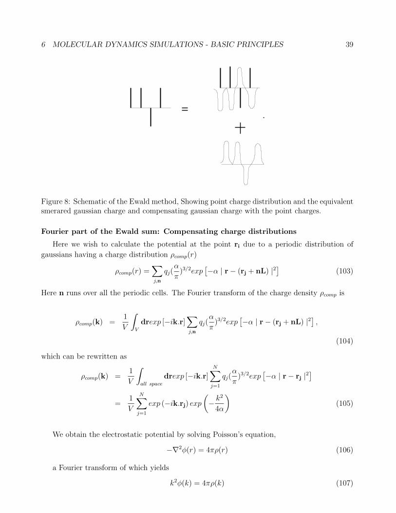
6 MOLECULAR DYNAMICS SIMULATIONS - BASIC PRINCIPLES 39
Figure 8: Schematic of the Ewald method, Showing point charge distribution and the equivalentsmerared gaussian charge and compensating gaussian charge with the point charges.
Fourier part of the Ewald sum: Compensating charge distributions
Here we wish to calculate the potential at the point ri due to a periodic distribution of
gaussians having a charge distribution ρcomp(r)
ρcomp(r) =∑j,n
qj(α
π)3/2exp
[−α | r− (rj + nL) |2
](103)
Here n runs over all the periodic cells. The Fourier transform of the charge density ρcomp is
ρcomp(k) =1
V
∫V
drexp [−ik.r]∑j,n
qj(α
π)3/2exp
[−α | r− (rj + nL) |2
],
(104)
which can be rewritten as
ρcomp(k) =1
V
∫all space
drexp [−ik.r]N∑j=1
qj(α
π)3/2exp
[−α | r− rj |2
]=
1
V
N∑j=1
exp (−ik.rj) exp(− k
2
4α
)(105)
We obtain the electrostatic potential by solving Poisson’s equation,
−∇2φ(r) = 4πρ(r) (106)
a Fourier transform of which yields
k2φ(k) = 4πρ(k) (107)
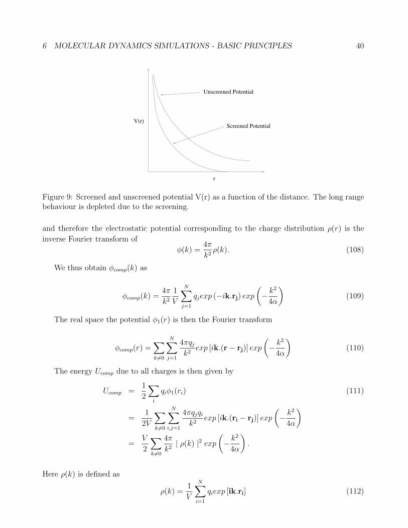
6 MOLECULAR DYNAMICS SIMULATIONS - BASIC PRINCIPLES 40
V(r)
r
Screened Potential
Unscreened Potential
Figure 9: Screened and unscreened potential V(r) as a function of the distance. The long rangebehaviour is depleted due to the screening.
and therefore the electrostatic potential corresponding to the charge distribution ρ(r) is the
inverse Fourier transform of
φ(k) =4π
k2ρ(k). (108)
We thus obtain φcomp(k) as
φcomp(k) =4π
k2
1
V
N∑j=1
qjexp (−ik.rj) exp(− k
2
4α
)(109)
The real space the potential φ1(r) is then the Fourier transform
φcomp(r) =∑k 6=0
N∑j=1
4πqjk2
exp [ik.(r− rj)] exp
(− k
2
4α
)(110)
The energy Ucomp due to all charges is then given by
Ucomp =1
2
∑i
qiφ1(ri) (111)
=1
2V
∑k 6=0
N∑i,j=1
4πqjqik2
exp [ik.(ri − rj)] exp
(− k
2
4α
)=
V
2
∑k 6=0
4π
k2| ρ(k) |2 exp
(− k
2
4α
).
Here ρ(k) is defined as
ρ(k) =1
V
N∑i=1
qiexp [ik.ri] (112)

6 MOLECULAR DYNAMICS SIMULATIONS - BASIC PRINCIPLES 41
Correction for Self Interaction
The previous calculation yields an extra term due to the interaction between the Gaussian
distribution centered at the location the point charge. The charge distribution that is over
counted is
ρGauss(r) = qi(α/π)3/2exp[−αr2
](113)
The Poisson equation is given by
−1
r
∂2φGauss(r)
∂r2= 4πρGauss(r) (114)
Substituting for ρGauss and integerating twice we have
φGauss(r) = qierf(√αr) (115)
Here erf(x) is the error function. The spurious contribution is at r = 0. Thus the total self
energy is
Uself =1
2
N∑i=1
qiφself (ri)
= (α
π)1/2
N∑i=1
q2i
(116)
Interaction of screened charges
This term is straighforward based on the previously obtained expressions. If the charge is
qi with the oppositely charged screening gaussian would yield a net potential of
φscreened(r) =qir− qirerf(√αr)
=qirerfc(
√αr) (117)
The net potential due to this term is thus
Uscreened =1
2
∑i,j
qiqjerfc(√αr)/rij (118)
The Ewald Sum Energy
Combining all the previous terms we have
6 MOLECULAR DYNAMICS SIMULATIONS - BASIC PRINCIPLES 42
UCoul =V
2
∑k 6=0
4π
k2| ρ(k) |2 exp
(− k
2
4α
)(119)
− (α
π)1/2
N∑i=1
q2i
+1
2
∑i 6=j
qiqjerfc(√αr)/rij
(120)
Note that the choice of α allows us to tune the range in real space of the screened interactions
(which increases if α decreases), which is balanced by the number of k points we need to keep
to to achieve a given accuracy, which increases if α increases.
The following exercise (Exercise 10, Chapter 4, Frenkel and Smit) takes us through a basic
(NVE) molecular dynamics program, and the quantities that one typically studies through a
molecular dynamics program.
Exercise 5: (Molecular Dynamics of a Lennard-Jones System)
A program has been made available that performs Molecular Dynamics (MD) for a Lennard-
Jones fluid in the NV E ensemble. Unfortunately,the program does not conserve the total energy
because it contains three errors.
1. Find the three errors in the code. Hint: there are two errors in integrate.f (integrate.c)
and one in force.f (force.c). See the file system.inc (system.h) for documentation about
some of the variables used in this code.
2. How is one able to control the temperature in this program? After all, the total energy of
the system should be constant (not the temperature).
3. To test the energy drift ∆U of the numerical integration algorithm for a given time step
∆t after N integration steps, one usually computes
∆U(∆t) =1
N
i=n∑i=1
∣∣∣∣U(0)− U(i∆t)
U(0)
∣∣∣∣In this equation, U (x) is the total energy (kinetic+potential) of the system at time x.
Change the program, only in mdloop.f (mdloop.c), in such a way that U is computed and
make a plot of U as a function of the time step. How does the time step for a given energy
drift change with the temperature and density?
6 MOLECULAR DYNAMICS SIMULATIONS - BASIC PRINCIPLES 43
4. One of the most time consuming parts of the program is the calculation of the nearest
image of two particles. In the present program, this calculation is performed using an
if-then-else-endif construction. This works only when the distance between two particles
is smaller than 1.5 and larger than -1.5 times the size of the periodic box. A way to
overcome this problem is to use a function that calculates the nearest integer nint
x = x− box nint(x/box)
Which expression is faster? (Hint: You only have to make some modifications in force.f
or force.c) Which expression will be faster on a vector computer like a Cray C90? Because
the nint function is usually slow, you can write your own nint function. For example,
whenx > −998, we can use
nint(x) = int(x+ 999.5)− 999
What happens with the speed of the program when you replace the standard nint function?
Do you have an explanation for this?
5. The equation x = x− box nint(x/box) can be written as x = x− box nint(x ibox) where
ibox is used instead of 1/box. Why would one do this?
6. An important quantity of a liquid or gas is the so called self diffusivity D. There are two
methods to calculate D:
(a) by integrating the velocity autocorrelation function:
D =1
3
∫ ∞0
< v(t).v(t+ t′) > dt
′
=1
3N
∫ ∞0
i=N∑i=1
< v(i, t).v(i, t+ t′) > dt
′(121)
(122)
in which N is the number of particles and v(i, t) is the velocity of particle i a time t. One
should choose t in such a way that independent time origins are taken, i.e. t = ia∆t,
i = 1, 2, . . . , and < v(t)v(t+ a∆t) >∼ 0. (why?).
(b) by calculating the mean square displacement:
D = limt′→∞
1
6t′<∣∣∣x(t+ t
′)− x(t)
∣∣∣2 >One should be very careful with calculation of the mean square displacement when particles
are always transformed to the central box (why?).

6 MOLECULAR DYNAMICS SIMULATIONS - BASIC PRINCIPLES 44
Modify the program in such a way that the self diffusivity can be calculated using both
methods. Only modifications in subroutine sample diff.f are needed. Why is it important
to use only independent time origins for the calculation of the means square displacement
and the velocity autocorrelation function? What is the unit of D in SI units? How can
one transform D into dimensionless units?
7. For Lennard-Jones liquids, Naghizadeh and Rice (J. Chem. Phys., 1962, 36, 2710-2720)
report the following equation for the self diffusivity (dimensionless units, T ∗ < 1.0 and
p∗ < 3.0)
10log(D) = 0.05 + 0.07p∗ − 1.04 + 0.1p∗
T ∗.
Try to confirm this equation with simulations. How can one translate D to a diffusivity
in SI units?
8. Instead of calculating the average energy < U > directly, one can use the radial distribu-
tion function g(r). Derive an expression for < U > using g(r). Compare this calculation
with a direct calculation of the average energy. A similar method can be used to compute
the average pressure.
9. In the current version of the code, the equation of motion are integrated by the Verlet
algorithm. Make a plot of the energy drift U for the following integration algorithms:
– Euler (never use this one except here !!!)
– Verlet
– Velocity Verlet
7 MOLECULAR DYNAMICS IN VARIOUS ENSEMBLES 45
7 Molecular dynamics in various ensembles
So far, we have discussed molecular dynamics in the microcanonical (N, V, E) ensemble. As
mentioned above in the context of Monte Carlo, it is useful to consider simulations in different
ensembles, and these considerations apply also to molecular dynamics. The manner in which
one generates such simulations is different in the case of molecular dynamics. Here we describe
the methods for performing molecular dynamics in a the (N,V,T) and (N,P,T) ensembles.
7.1 Molecular Dynamics in the (N, V, T ) ensemble:
Since we measure the temperature in molecular dynamics simulations from the total kinetic en-
ergy, one possibility to attempt constant temperature simulations is to modify the equation of
motion such that the total kinetic energy is conserved. Such methods, however, do not generate
a true canonical ensemble. Another possibility that has been proposed is to stochastically alter
the velocities of particles in addition to the deterministic equations of state, so that a canon-
ical ensemble is reached, using the so called “Andersen thermostat”. Though the equilibrium
ensemble desired is obtained, the dynamics using this method is seen to be strongly dependent
on the thermostat parameter. A general scheme, that is widely applicable to generating dif-
ferent ensembles is the extended Lagrangian method, whereby one considers the system with
additional degrees of freedom not present in the microscopic Hamiltonian. The Nose-Hoover
thermostat is described here that achieves a constant temperature ensemble. The extended
Lagrangian of the system is written as:
LNose =N∑i=1
mi
2s2r2
i − U(rN) +Q
2s2 − L
βln s, (123)
where s is a new degree of freedom and Q is the effective mass associated with it. L will be
determined later. The conjugate momenta of variables r and s are given by:
pi =∂L∂r
= mis2ri (124)
and
ps =∂L∂s
= Qs. (125)
The corresponding Hamiltonian is
HNose =N∑i=1
p2i
2mis2+ U(rN) +
p2s
2Q+ L
ln s
β. (126)

7 MOLECULAR DYNAMICS IN VARIOUS ENSEMBLES 46
The partition function for this system is
QNose =1
N !
∫dps ds dp
N drNδ(E −HNose). (127)
We define p′= p/s and
H =N∑i=1
p′ 2i
2mi
+ U(rN). (128)
Using the relation
δ(h(s)) = δ(s− s0)/h′(s0)
when h(s) is a function that has only one root at s0, we can write
QNose =1
N !
∫dps ds dp
′N drNβ s3N+1
Lδ
s− exp
[−βH(p
′, r) + p2s
2Q− E
L
]. (129)
With the choice of L = 3N + 1, this simplifies to
QNose =C
N !
∫dp
′N drN exp[−βH(p
′, r)]
(130)
which is the canonical ensemble. From the above, the primed variables are the real variables,
and are related to the unprimed ones by r′
= r, p′
= p/s, s′
= s, p′s = ps/s, and t
′= t/s. The
dynamical equations for these variables can be written, using the Hamiltonian HNose as
dr′i
dt′= p
′
i/mi (131)
dp′i
dt′= −∂U
∂r′i
− (s′p′
s/Q)p′
i
1
s
ds′
dt′= s
′p′
s/Q
d(s′p′s/Q)
dt′=
(∑i
p′2i /mi −
3N + 1
β
)/Q.
These equations conserve
HNose =N∑i=1
p′2i
2mi
+ U(r′N) +
s′2p
′2s
2Q+ L
lns′
β. (132)

7 MOLECULAR DYNAMICS IN VARIOUS ENSEMBLES 47
7.2 Molecular Dynamics in the (N,P, T ) ensemble:
Along the same lines as the constant temperature case, one can write an extended Lagrangian
for the isothermal-isobaric case, where we will now have two additional variables instead of one
before. The equations of motion for the positions and momenta are given by
ri =pimi
+pεW
ri, (133)
pi = Fi − (1 +1
N)pεW
pi −pξQ
pi. (134)
The variable that defines the volume is, ε = ln(V/V0) and the equations of motion for the
volume and the corresponding momentum are written as:
V =d V pεW
, (135)
pε = d V (Pint − Pext) +1
N
N∑i=1
p2i
mi
− pξQpε, (136)
where the Pint is the “internal” pressure calculated from the virial and the kinetic energy
of the system, and Pext is the external, imposed pressure.
8 ANALYSIS OF DATA: STATISTICS AND ERROR ESTIMATION 48
8 Analysis of data: Statistics and Error Estimation
In principle, a Monte Carlo or a Molecular Dynamics simulation will provide estimates of
ensemble averages that are exact in the sense that no approximations such at those often made
in analytical calculations are involved. However, there are clearly identifiable sources of error
in our estimates. Very broadly, errors in simulations arise from (a) the model (how good is the
Hamiltonian we use to describe the system we want to describe), (b) finite size, and (c) finite
sampling. We will not discuss the first of these sources of error, but focus on estimation of
properties for a chosen model system, and in particular errors arising from finite sampling.
Consider that we are calculating the average of a property A. The exact average value is
given by an average over an infinitely long trajectory or equivalently over an infinitely large
sampling. We don’t have this luxury, so let us consider a finite time average
Aτ =1
τ
∫ τ
0
dtA(t). (137)
It is clear that if we perform many different ”runs”, each time of length τ , we will have differ-
ent results. The error of a finite estimate may be quantified by the variance of the distribution
of these different estimates:
σ2(Aτ ) =< A2τ > − < Aτ >
2 (138)
This is equal to
σ2(Aτ ) =1
τ 2
∫ ∫dtdt
′< (A(t)− < A >)(A(t
′)− < A >) (139)
Defining the correlation function CA(t) as
CA(t) =1
τ
∫dt
′< (A(t
′+ t)− < A >)(A(t
′)− < A >) (140)
and assuming the form CA(t) = (< A2 > − < A >2) exp(−t/tc) and that tc) << τ , we have
σ2(Aτ ) =2
τ
∫ ∞0
dtCA(t) =2tcτCA(0). (141)
The relative error is therefore quantified by
σ2(Aτ ) =2tcτ
(< A2 > − < A >2)
< A >2. (142)
Thus, we see that the error in our estimate decreases with tcτ
which is equal to the number
of independent samples. The quality of the estimate therefore depends on the length of the run

9 HISTOGRAM METHODS 49
in units of the relaxation time. However, we do not have the estimate of the relaxation time a
priori. But we can estimate the relaxation time by considering the fact that the quantity
R(τ) =σ2(Aτ ) ∗ τ
2(< A2 > − < A >2)(143)
will approach the relaxation time for long enough τ . Alternately, we can see that the
variance will be inversely proportional to the number of blocks over which we average whereas
for τ < tc this will not be the case.
Rigorous statistical analysis is usually easier post facto and many rules of thumb are used to
ensure that a given simulation is satisfactory by considering physically motivated measures such
as the mean squared displacement of particles over a given time segment etc. These measures
are usually recipes for estimating a relevant relaxation time in a practical and efficient way.
9 Histogram Methods
So far we have been evaluating averages of quantities using MC. However, in the process we
do obtain information about the distributions (in energy or any other parameter of relevance).
Can this information be used? As a simple example, consider that one is simulating the system
at a given temperature T0. We can calculate the histogram of the energies sampled by, H(E)
given N samples. Then, the probability of energy E is given by P0(E) = H0(E)/N . However,
if we have a distribution of states or density of states W (E) for the system, we have
H0(E) =N
Z0
W (E) exp(−β0E) (144)
From this, we can write an estimate of the histogram W as
W (E) =Z0
NH0(E) exp(β0E). (145)
Knowing W (E), we can write the distribution at any other temperature T1 as
P1(E) =1
Z1
W (E) exp(−β1E). (146)
Substituting for W (E),
P1(E) =Z0
NZ1
H0(E) exp((β0 − β1)E). (147)
We do not however know the normalization Z0/Z1. But this can be imposed by explicitly
normalizing P1. Thus,

9 HISTOGRAM METHODS 50
P1(E) =H0(E) exp[(β0 − β1)E]∑E H0(E) exp[(β0 − β1)E]
. (148)
This will work when we consider T0 and T1 such that the region of sampling in the two
cases overlap substantially. We can expect that when this is not the case, this method will not
work so well. In such cases, we may employ methods for improved sampling, such as umbrella
sampling.
Exercise 6
Consider the earlier exercise of simulating the Ising model with J = 0, in a magnetic field
B = 1. Perform the simulation at T = 4 and obtain the histogram of energies (in this
case, this is simply given by the magnetization n M = 1N
∑i Si). Varying the temperature
from T = 4 to T = 0.1, calculate the re weighted histograms from that obtained at T = 4.
Compare with the results obtained directly by simulating at the respective temperatures.
9.1 Umbrella Sampling
In order to discuss umbrella sampling, first we consider again two systems 0 and 1, with
interaction energies U0 and U1. Then, we have the free energy difference between them is given
by
β∆F = − log(Z1/Z0). (149)
We now consider calculating both the energies U0 and U1 during simulations of each of the
states 0 and 1, and to evaluate ∆U = U1−U0. The normalized distribution of ∆U for the state
1 is given by
p1(∆U) =1
Z1
∫drN exp(−βU1)δ(U1 − U0 −∆U). (150)
Since the integral is finite for U1 = U0 + ∆U we can substitute for U1 and we have
p1(∆U) =exp(−β∆U)
Z1
∫drN exp(−βU0)δ(U1 − U0 −∆U). (151)
We can rewrite this in terms of an average over the state 0 and therefore
p1(∆U) = exp(−β∆U)Z0
Z1
p0(∆U) (152)
with
p0(∆U) =1
Z0
∫drN exp(−βU0)δ(U1 − U0 −∆U). (153)
9 HISTOGRAM METHODS 51
Finally, noting that β∆F = − log(Z1/Z0) we have
p1(∆U) = exp[β(∆F −∆U)]p0(∆U). (154)
Thus, we can write the free energy as
β∆F = [log p1(∆U)]− [log p0(∆U)−∆U ]. (155)
Therefore we can calculate ∆F by considering the constant difference between the two
quantities on the right hand side. For simplicity, we define
f0(∆U) = log p0(∆U)− β∆U/2 (156)
and
f1(∆U) = log p1(∆U) + β∆U/2 (157)
With these,
β∆F = f1(∆U)− f0(∆U). (158)
As a specific example, consider that we have a N particle system and U1 corresponds to
this N particle system, and 0 corresponds to the case where (N − 1) particles have the desired
interaction, and one of the particles does not interact with the rest of the system (i.e. it is an
ideal gas particle). In this case, the difference in the free energy is the excess chemical potential,
and the integration of the result above can be seen to give the Widom insertion method. The
difference here is that the full distribution is being used, which gives, among other things, a
check on the reliability of the method.
However, in order for this method to work, the range over which p1(∆U) and exp(−β∆U)p0(∆U)
have significant weight must overlap. This cannot always be guaranteed in the scheme above
and the results can be subject to large sampling error. Umbrella sampling is a method that
attempts to improve the accuracy of such estimates by ensuring that one has adequate sam-
pling over a desired range of property values. Considering the expression for the free energy
difference, we can write it explicitly as
exp[−β∆F ] =
∫drN exp(−βU1)∫drN exp(−βU0)
(159)
Now consider that we sample not according to the weights exp(−βU1) or exp(−βU0) but
from a presently unspecified distribution w(rN). We can rewrite the above expression for the
free energy as
9 HISTOGRAM METHODS 52
exp[−β∆F ] =
∫drNw(rN)[exp(−βU1)/w(rN)]∫drNw(rN)[exp(−βU0)/w(rN)]
(160)
or
exp[−β∆F ] =< [exp(−βU1)/w(rN)] >w
< [exp(−βU0)/w(rN)] >w
(161)
where < .. >w indicates an average over the ensemble defined by w(rN). What has been gained
by this? The answer lies in our ability to choose a suitable w(rN), so that we can sample the
relevant configuration space properly, for the evaluation of the averages involved. This requires
some knowledge of the system under study. Examples of the application of this method will be
discussed later in the course.
9.2 Histogram Reweighting or Multi-Histogram Method
In the introduction, we described a way of reweighting a single historgram obtained from one
simulation to obtain the distribution at a different state point. We can extend this method
(Ferrenberg and Swendsen 1989) whereby we use the histogram data from multiple histograms
and try to generate an estimate for the density of states W or equivalently the probability
density Pn(E) where n denotes an arbitrary chosen state. For this we wish to generalize the
reweighting scheme for the single histogram case :
P1(E) =Z0
NZ1
H0(E) exp((β0 − β1)E) (162)
which we can rewrite as
P1(E) =1
Z1
H0(E)
N exp(−β0E)Z−10
exp((−β1)E) (163)
to a situation where we have multiple histograms. The corresponding generalization is
Pn(E) =
∑mj=1 g
−1j Hj(E)∑
j Njg−1j exp(−βjE + fj)
exp(−βnE) (164)
The factors fj have to be obtained self consistently, using
exp(−fn) =∑E
Pn(E). (165)
These factors therefore yield the free energy.

9 HISTOGRAM METHODS 53
9.3 Wang-Landau Algorithm
In the Wang-Landau algorithm, one generates states not using the Boltzmann weight but
according to a modified weight such that the histogram of states generated is flat in the chosen
parameter, say the energy. Consider
Z =∑E
g(E) exp(−βE) (166)
where g(E) is the density of states. Suppose we want to choose the ”weight” exp(−βE) such
that all energies have equal weight. Then we would need to choose the weight to be proportional
to g(E)−1. The problem is that we do not know g(E). On the other hand, if we did know it,
we can evaluate the partition function and all properties of interest at any state point. The
Wang-Landau algorithm uses the update scheme
p(E1 → E2) = min (g(E1)/g(E2), 1) (167)
where p is the acceptance probability. Since we do not know g(E) to begin with, it is set to 1.
Each time a state with energy E is visited, we modify
g(E) = g(E)ofi (168)
where fi is a multiplicative factor that is set to some number (f0 = e for example). During
the Monte Carlo simulation, a histogram of visited states is accumulated. When the histogram
becomes flat according to a chosen criterion, the next iteration is initiated, which involves (i)
reducing fi to fi+1 = f1/2i for example, and (ii) reinitiating the histogram. The next iteration
is started with the current estimate of g(E). This process is repeated till f become sufficiently
small fmin = 10−8 for example). This results in a density of states g(E) that can be used for
calculating properties of interest.

10 FREE ENERGY CALCULATION AND PHASE EQUILIBRIA 54
10 Free Energy calculation and phase equilibria
The methods discussed so far have allowed us to calculate averages such as the internal energy
and pressure. However, for many simulation studies, such as the study of phase transitions, one
would like to have access to free energies. Free energies cannot be obtained as simple minded
averages from MD or MC simulations, since they are not given by averages of functions of
phase space coordinates, but also involve information about the phase space volume accessible
to the system. Nevertheless, they can indeed be calculated quite straightforwardly. Some of
the methods for such calculations are described here.
10.1 Thermodynamic Integration:
The basic idea of this method is very simple. Quantities such as pressure and internal energies
are given by derivatives of, e. g., the Helmholtz free energy.(∂F
∂V
)N,T
= −P, (169)
(∂ βF
∂β
)N,V
= U. (170)
Thus, if one has measured values of pressure or internal energy along a reversible path that
connects the state point of interest to a state of known free energy, a numerical integration will
give us the desired free energy. For example, integrating the pressure along an isotherm from
density approaching zero to the required density will yield the free energy at that point, by
making use of the known free energy of the ideal gas.
However, in simulations, we are not restricted to using standard thermodynamic derivatives.
A general scheme for using thermodynamic integration can be developed by considering a
potential energy function that is a linear combination of the potential energy in the desired
system, and the reference system. We write
U(λ) = (1− λ)UI + λUII = UI + λ(UII − UI), (171)
so that when λ = 0, U(λ) corresponds to the potential of the reference system I, whereas for
λ = 1, it corresponds to the potential for the system we wish to study. The partition function
can be written as a function of λ, as
Q(N, V, T, λ) =1
Λ3NN !
∫drN exp[−βU(λ)]. (172)
Taking the derivative with respect to λ,
10 FREE ENERGY CALCULATION AND PHASE EQUILIBRIA 55
(∂F (λ)
∂λ
)N,V,T
=
∫drN
(∂U(λ)∂λ
)exp[−βU(λ)]∫
drN exp[−βU(λ)](173)
=
⟨∂U(λ)
∂λ
⟩λ
.
Therefore, integrating both sides,
F (λ = 1)− F (λ = 0) =
∫ λ=1
λ=0
dλ
⟨∂U(λ)
∂λ
⟩λ
. (174)
This equation can be used, by evaluating⟨∂U(λ)∂λ
⟩λ
for values of λ between 0 and 1, to
evaluate the desired free energy by numerical integration. For the choice of U(λ) above, we
have ⟨∂U(λ)
∂λ
⟩λ
= 〈(UII − UI)〉 . (175)
With the chosen form of U(λ), we have a convenient check on the simulations that we
perform, in the form of the second derivative of F (λ) with λ, which is guaranteed to be negative:(∂2F (λ)
∂λ2
)N,V,T
= −β< (UII − UI)2 >λ − < (UII − UI) >2
λ
≤ 0. (176)
10.2 Widom Insertion Method for Chemical Potential:
The chemical potential is a very useful quantity to calculate, as it allows us to judge conditions
for phase coexistence and relative stability of phases. We have the thermodynamic identity,
µ =
(∂F
∂N
)V,T
, (177)
which we now write in terms of the partition functions of a N particle and N + 1 particle
system. The free energy is given by
F (N, V, T ) = −kBT logQ (178)
= −kBT log
(V N
Λ3NN !
)− kBT log
[∫dsN exp(−βU(sN ;L)
]= Fid(N, V, T ) + Fex(N, V, T ).

10 FREE ENERGY CALCULATION AND PHASE EQUILIBRIA 56
The last equation defines the ideal gas and the excess contributions to the free energy. Now
we write µ as
µ = −kBT log(QN+1/QN) (179)
= −kBT log
(V
Λ3N + 1
)− kBT log
[∫dsN+1 exp(−βU(sN+1;L)∫dsN exp(−βU(sN ;L)
]= µid + µex.
The expression for the excess chemical potential can be thought of the average of exp(−β∆U)
over the N particle canonical ensemble, where ∆U = U(N + 1)−U(N) is the difference in the
energy of an N particle system, and an N + 1 particle system. Thus,
µex = −kBT log
∫dsN+1 < exp(−β∆U) >N . (180)
In order to calculate this, we need to average over all positions of the (N + 1)th particle. This
we do by sampling, as follows. We perform a N particle canonical Monte Carlo simulation.
Periodically, we generate random coordinates for the (N + 1)th particle, and we calculate the
interaction energy an additional particle at that location would have with the rest of the
system. For systems which are not too dense, this method provides a good way of calculating
the chemical potential.
10.3 Phase Equilibria: The Gibbs Ensemble Method:
The Gibbs ensemble technique is a useful method for calculating the location of a first order
phase transition. In discussing the method, we will keep in mind a liquid-gas phase transition.
Experimentally, the condition for coexistence at a given temperature (assuming that it is below
the critical temperature) is that the coexisting phases have the same pressure and the chemical
potential. Experimentally, such a coexistence is achieved when the two phases are separated
by a boundary, across which particle, energy and volume exchange is possible. In simulations,
given the sizes of the simulation cells, we do not want to consider two phase systems, which
would have a very large fraction of the system residing at the boundary, but we would like
to retain the possibility of exchange of volume and particles between two subvolumes, so that
they can reach coexistence. This is achieved in the Gibbs ensemble simulations by considering
a system that is a canonical system specified by a given N, V, T. We consider this system to be
made of two subsystems, which can exchange particles and also volume, with the sum adding
always to N, V respectively. We can write the total partition function for the system as
Q(N, V, T ) =N∑
n1=0
1
V Λ3Nn1!(N − n1)!
∫V
dV1Vn1
1 (V − V1)(N−n1) (181)
×∫dsn1
1 exp[−βU(sn11 )]
∫dsN−n1
2 exp[−βU(sN−n12 )].
10 FREE ENERGY CALCULATION AND PHASE EQUILIBRIA 57
The probability density for a specific configuration where the first subsystem has n1 particles
in volume V1 is
N (n1, V1, sn11 , s
N−n12 ) ∝ V n1
1 (V − V1)(N−n1)
n1!(N − n1)!exp[−β(U(sn1
1 ) + U(sN−n12 ))] (182)
With this probability, we sample configurations with the following set of moves:
1. Displacement of randomly selected particles in each subsystem. This is governed by the
standard Metropolis algorithm.
2. Change the volume of each subsystem in such a way that that total remains constant. We
can implement this either by making a change in the volume or in the log of the volume.
The acceptance probability in the two cases will be:
acc(o→ n) = min
[1,
(V n1 )n1(V − V n
1 )N−n1
(V on )n1(V − V o
1 )N−n1exp(−β[U(sNn )− U(sNo )]
]. (183)
and
acc(o→ n) = min
[1,
(V n1 )n1+1(V − V n
1 )N−n1+1
(V on )n1+1(V − V o
1 )N−n1+1exp(−β[U(sNn )− U(sNo )]
]. (184)
3. Transfer a randomly selected particle from one box to the other. For removing a particle
from the first box and inserting it in the second, the acceptance probability for this is
given by:
acc(o→ n) = min
[1,
n1(V − V1)
(N − n1 + 1)V1
exp(−β[U(sNn )− U(sNo )]
]. (185)
With these moves, we generate configurations in the two subsystems that correspond to two
coexisting phases. The equilibrium condition can independently be verified by calculating the
pressure and the chemical potential and ensuring that they are equal.
10.4 Gibbs-Duhem Integration
In many systems, using a method such as the Gibbs ensemble method to determine the phase
coexistence lines may be computationally demanding. An example is the liquid-solid coexistence
line, which is difficult to determine because of the difficulty of insertion. In such cases, a method
such as the Gibbs-Duhem integration is useful. The method is based on a clever use of the
Clausius-Clapeyron equation,

10 FREE ENERGY CALCULATION AND PHASE EQUILIBRIA 58
dP
dT=s1 − s2
v1 − v2
=∆h
T∆v(186)
as a condition for phase equilibrium. Here s1, s2 are the entropies of the two phases in co-
existence, P is the pressure, T is the temperature, ∆h is the enthalpy difference, and ∆v is the
difference in volume. This can be derived from the Gibbs-Duhem relation
dµ = −sdT + vdP (187)
which gives the method its name. Once a point on the phase coexistence line has been de-
termined, the Clausius-Clapeyron equation provides an equation that can in principle be in-
tegrated to obtain the phase coexistence curve. This can be done using numerical techniques
for integration, and noting the fact that h and v can easily be calculated for the two phases as
averages.
11 OPTIMIZATION, BIASED AND ACCELERATED SAMPLING 59
11 Optimization, biased and accelerated sampling
So far we have assumed that the trial moves that we choose in a Monte Carlo simulation are
sufficient to ensure proper sampling. However, there are many situations when simple minded
trial moves will not bring the system to equilibrium in a reasonable time period. On the other
hand, in systems showing slow or “glassy” dynamics, even though the microscopic events can
be generated with ease, it will be found that the system is “stuck” in the same part of phase
space because it is not able to overcome barriers present in order for other parts of phase space
to be explored. In these cases, one resorts to augmented Monte Carlo schemes, which improve
the sampling qualitatively. In the former type of example (dense polymer melt), biased Monte
Carlo methods allow for the generation of sensible trial moves. One may also attempt to use
the natural dynamics of the system to general trial configurations for the Metropolis algorithm.
In other cases, one may take note of the correlations that exist in the system by generating
cluster moves. These methods will be discussed here.
Glassy systems are characterized by the fact that there are many local minima present in
the landscape of the system and the system can get stuck in one of them for a long time and
therefore prevent proper sampling. For glassy behavior, methods such as parallel tempering
allow for (free) energy barriers to be overcome so that the system explores phase space efficiently.
There are two problems that can be distinguished here. One may simply want to find low (or
the lowest) energy configurations. This class of problems are optimization problems. The other
is the problem of overcoming these barriers to achieve proper sampling. We discuss simulated
annealing and parallel tempering as suitable methods for these two classes of problems.
11.1 Simulated Annealing
Simulated annealing is a method that applies a ”common sense” physical approach to generating
optimized configurations (e. g. of atoms in a metal) by equilibrating the system at a high
temperature so that the atoms have enough mobility to rearrange and eliminate defects that
may cause degradation of material properties. The temperature is changed to lower values
gradually, so that successively lower energy configurations are achieved. Such a method can
also be employed to find optimum solutions even when the system under consideration is not
a thermal system. The classic problem in computer science is the traveling salesman problem.
The problem is for a salesman to visit N cities, and returning to the point of departure after N
steps, in such a way that the total distance traveled is minimum. There is no energy function
in the normal sense in this problem but the ”cost” function that needs to be minimized is
E =N∑i=1
√(xi − xi+1)2 + (yi − yi+1)2 (188)
Simulated annealing involves defining a schedule of cooling or annealing such that one per-
forms a Monte Carlo simulation using the above energy function at successively lower temper-

11 OPTIMIZATION, BIASED AND ACCELERATED SAMPLING 60
atures.
11.2 Parallel Tempering:
In many systems, the time evolution of particle coordinates at low temperatures is characterized
by long periods of time when the system is localized among configurations that are not very
different from each other, and transitions to other equivalent (in terms of structure, macroscopic
properties like energy etc) configurations take long waiting times. Such a situation is described
by saying that the system exhibits many local free energy minima that are separated by large
barriers. Since the proper sampling of phase space requires the system to sample many such
free energy minima, one needs methods that allow the system to make transitions between such
minima efficiently. A typical example of this situation is a dense liquid at low temperatures
where it will eventually undergo the glass transition. At temperatures close to but above the
glass transition, the times scales for structural relaxation in these liquids becomes very large.
In parallel tempering, one approaches a solution to this problem by considering the system
not at a single temperature but for a range of temperatures (here, we will discuss only the case
where temperature is varied, though other possibilities also exist. We also consider systems
to be simulated in the canonical ensemble). Let us suppose that at the highest temperatures
considered, the system is able to freely explore phase space, whereas at the low temperature
end, the system gets stuck if we were to perform a simple canonical ensemble simulation.
We can write the partition function for the set of all the systems at all the temperarures:
Qparallel = Πni=1Q(N, V, Ti) = Πn
i=1
1
Λ3Ni N !
∫drNi exp(−βiU(rNi )). (189)
We can of course simulate this system by performing canonical Monte Carlo for each tem-
perature independently. In parallel tempering, we do that, but in addition, we periodically swap
configurations between successive temperatures. Consider two inverse temperatures β1 and β2.
Let the configuration of particles for the ensembles being generated at these temperatures be
represented by 1 and 2. The detailed balance condition for a swap of the configurations is given
by
N (1, β1) N (2, β2) α((1, β1), (2, β2)→ (2, β1)(1, β2)) (190)
× acc((1, β1), (2, β2)→ (2, β1)(1, β2)) =
N (2, β1) N (1, β2) α((2, β1), (1, β2)→ (1, β1)(2, β2))
× acc((2, β1), (1, β2)→ (1, β1)(2, β2)).
N (1, β1) ∝ exp(−β1U(1) etc. If we periodically attempt a swap move, the probability of
forward and backward trials α are the same. Therefore, the acceptance ratio will be given by

11 OPTIMIZATION, BIASED AND ACCELERATED SAMPLING 61
acc((1, β1), (2, β2)→ (2, β1)(1, β2))
acc((2, β1), (1, β2)→ (1, β1)(2, β2))= exp[(β1 − β2)(U(1)− U(2))]. (191)
This can be achieved with
acc((1, β1), (2, β2)→ (2, β1)(1, β2)) = min(1, exp[(β1 − β2)(U(1)− U(2))]). (192)
It is clear that the probability of acceptance is higher the closer together the temperatures
are, and the distribution of energies in the ensembles between which we attempt a swap is
non-negligible. In addition to the canonical case considered here, it is possible to extend the
parallel tempering scheme to other cases.
11.3 Configurational Bias Monte Carlo:
The example we consider here is a polymer chain in a polymer melt. For the sake of simplicity,
we will imagine that these polymers sit on a lattice, where each monomer sits at a cell on a
lattice, as shown in Figure. 10) If we were to perform molecular dynamics, the entanglement
of the polymer will impose barriers to its movement. In a Monte Carlo simulation, an attempt
to generate trial configurations will require generating the positions for all the monomers of
a polymer, and a randomly generated polymer configuration, for a dense enough melt, have
an overwhelming probability of overlapping with another polymer chain in the system. Thus,
we need another method whereby the chain is generated. We describe here the configurational
bias Monte Carlo method that achieves this.
The method uses the so called Rosenbluth scheme for generating polymer conformations (of
length l). As we will see, the conformations generated will have a probability that depends on
the energy of the conformation. Let us represent it by writing
α(o→ n) = f [U(n)]. (193)
Given such a generation probability, in order for us to ensure detailed balance, we much
modify the acceptance probability such that
acc(o→ n)
acc(n→ o)=f [U(o)]
f [U(n)]exp[−β(U(n)− U(o))]. (194)
This can be achieved by choosing
acc(o→ n) = min(1,f [U(o)]
f [U(n)]exp[−β(U(n)− U(o))]). (195)
Thus, the bias that is introduced at the time of generating a conformation is rectified at the
time of acceptance.
Next we have to evaluate the bias in the Rosenbluth scheme, which is outlined here:

11 OPTIMIZATION, BIASED AND ACCELERATED SAMPLING 62
1. The first monomer is inserted at a random position, and its energy is denoted by u1(n).
We associate a Rosenbluth weight for this monomer as w1 = exp(−βu1(n)).
2. For subsequent monomers, we consider k possible positions (in the case of a lattice poly-
mer, all k positions that are allowed; a uniform sample for off-lattice). Denoting the energy
of the jth possibility by ui(j), we select the possibility we denote by n with probability
pi(n) = exp(−βui(n))/wi
where
wi =k∑j=1
exp(−βui(j)).
The energy we count is the energy of the new monomer with all the pre-existing monomers
and other polymers in the system. Hence, the total energy of the full chain is given by
U(n) =∑
i ui(n).
3. The Rosenbluth factor is computed as
W (n) = Πli=1wi.
From these, the probability distribution of generating a given configuration n is clearly
P (n) = Πli=1
exp(−βui(j))wj
=exp(−βU(n))
W (n).
This probability is normalized. If we generate a number of configurations from such a
method, since the configurations are generated with probability P (n) rather than simply
exp(−βU(n)), in order to calculate the average over these conformations that obeys the Boltz-
mann distribution, we have to weigh each of the configurations with W (n), ie
< A >R=
∑nW (n)A(n)∑
nW (n)=
∑nA(n) exp(−βU(n))∑
n exp(−βU(n))=< A > .
Now, to use the Rosenbluth scheme to perform CBMC, which has three steps:
1. Generate a trial configuration and compute the Rosenbluth weight W (n). Note that the
generation probability is exp(−βU(n))W (n)
.
2. For the old conformation, in order to calculate the Rosenbluth factor W (o) by retracing
the Rosenbluth procedure in reverse.
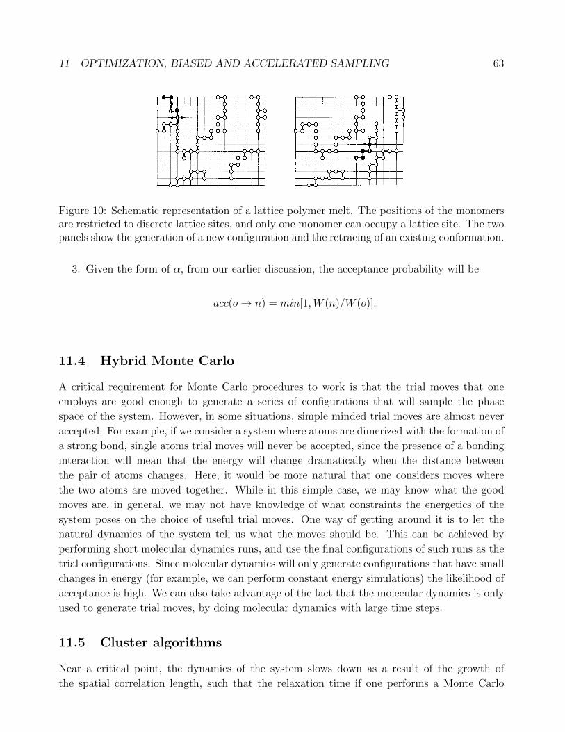
11 OPTIMIZATION, BIASED AND ACCELERATED SAMPLING 63
Figure 10: Schematic representation of a lattice polymer melt. The positions of the monomersare restricted to discrete lattice sites, and only one monomer can occupy a lattice site. The twopanels show the generation of a new configuration and the retracing of an existing conformation.
3. Given the form of α, from our earlier discussion, the acceptance probability will be
acc(o→ n) = min[1,W (n)/W (o)].
11.4 Hybrid Monte Carlo
A critical requirement for Monte Carlo procedures to work is that the trial moves that one
employs are good enough to generate a series of configurations that will sample the phase
space of the system. However, in some situations, simple minded trial moves are almost never
accepted. For example, if we consider a system where atoms are dimerized with the formation of
a strong bond, single atoms trial moves will never be accepted, since the presence of a bonding
interaction will mean that the energy will change dramatically when the distance between
the pair of atoms changes. Here, it would be more natural that one considers moves where
the two atoms are moved together. While in this simple case, we may know what the good
moves are, in general, we may not have knowledge of what constraints the energetics of the
system poses on the choice of useful trial moves. One way of getting around it is to let the
natural dynamics of the system tell us what the moves should be. This can be achieved by
performing short molecular dynamics runs, and use the final configurations of such runs as the
trial configurations. Since molecular dynamics will only generate configurations that have small
changes in energy (for example, we can perform constant energy simulations) the likelihood of
acceptance is high. We can also take advantage of the fact that the molecular dynamics is only
used to generate trial moves, by doing molecular dynamics with large time steps.
11.5 Cluster algorithms
Near a critical point, the dynamics of the system slows down as a result of the growth of
the spatial correlation length, such that the relaxation time if one performs a Monte Carlo

11 OPTIMIZATION, BIASED AND ACCELERATED SAMPLING 64
simulation will go as τ ∼ ξz (z ∼ 2 for the two dimensional Ising model) where ξ is the
correlation length. Apart from the interest in this ”critical slowing down” as a phenomenon,
one would like to find ways of getting around it in computer simulations. In lattice systems like
the Ising model (or the Potts model of which the Ising model can be viewed as a special case),
methods have been developed that employ ”cluster flipping” to beat critical slowing down. The
basic idea is the following. Consider the Hamlitonian
−βHPotts = K∑<ij>
(δσiσj − 1). (196)
This corresponds to
HPotts = −2J∑<ij>
(δσiσj − 1). (197)
and therefore, K = 2βJ (Compare with the Ising model where the difference in energy
between parallel and anti-parallel spin pairs is 2J). The partition function is given by
ZPotts =∑σ
exp[K∑<ij>
(δσiσj − 1)] (198)
It has been shown (Fortuin and Kasteleyn 1969, 1972) that the Potts model maps to the
percolation problem, with the critical behavior of the Potts model mapping to the percolation
transition. The mapping involves a bond occupation probability
p = 1− exp(−K) (199)
when two neighbor sites have the same state.
As the critical point is approached, the larger and larger clusters of spins that are correlated
thus map to the larger percolation clusters that would be generated under the above mapping.
It will become progressively harder to change the state of individual spins, and therefore one
may wish to consider collective changes in generating trial states. Algorithms that attempt to
do so involve identifying clusters of spins to ”flip” in such a way that the flipping can be done
with unit probability.
The Swendsen-Wang algorithm performs Monte Carlo using the following procedure:
• Consider all pairs of neighbor spins of the lattice, and insert a bond according to the
occupation probability p.
• Perform a cluster finding procedure to identify all clusters.
• For each cluster, change the Potts states to a randomly chosen new value, i. e. ”flip the
cluster”
11 OPTIMIZATION, BIASED AND ACCELERATED SAMPLING 65
This algorithm has been shown to reduce critical slowing down but it is not the most
efficient algorithm. The reason is that in this procedure one is treating all the clusters equally,
but small clusters do not contribute to critical slowing down. Instead, in the Wolff algorithm
one follows the following steps:
• Pick a random site. Draw bonds to all neighbors that have the same value of the Potts
variable σ with probability p = 1− exp(−K)
• Repeat the process for all the connected neighbors, till no more spins can be added.
• Flip all the Potts spins of the cluster.
In order to see that these algorithms will generate configurations with the desired equilibrium
distribution, we must demonstrate that the trial steps and acceptance criteria obey detailed
balance. To see this, let us consider the Ising model. The detailed balance condition involves
the generation step and the acceptance probability. As stated before we would like to define
the procedure such that the acceptance probability is 1. The generation step involves the
generation of a bond/cluster configuration, and given the bond configuration, the generation
of the new configuration. For either the Potts or the Ising model, it is easy to see that for a
given cluster, the cluster flipping step is symmetric, i. e. starting with either the old or the
new spin configuration, the probability of generating the other is the same (and equal to 1 for
the Ising model, and 1/(q − 1) for the Potts model). Therefore, the detailed balance condition
boils down to satisfying:
N (o)P oGen = N (n)P n
Gen (200)
orP oGen
P nGen
=N (n)
N (o)= exp[−β(En − Eo)] (201)
Let us consider that we have Np parallel spin pairs, and Na anti-parallel spin pairs. The
energy is
E = J(Na −Np). (202)
Let ∆ be the number by which the number of parallel spins increases as a result of the cluster
flipping. Thus, Np(n) = Np(o) + ∆ and Na(n) = Na(o)−∆. The change in energy is therefore
En − Eo = −2J∆ (203)
Now consider that out of Np pairs, we draw a bond for nc (connected) of them and do not
draw a bond for nb (broken). Thus Np(o) = nc(o) + nb(o). The probability of doing so is
P oGen = pnc(o)(1− p)nb(o) (204)

11 OPTIMIZATION, BIASED AND ACCELERATED SAMPLING 66
Now if we consider the new configuration, and the generation of the old configuration from
it, nc(n) = nc(o) since the number of parallel spin pairs that are connected does not change.
On the other hand, the number of ”broken” bonds changes, as we can see by considering that
Np(n) = nc(n) + nb(n) = nc(o) + nb(n) = Np(o) + ∆ = nc(o) + nb(o) + ∆. Thus,
nb(n) = nb(o) + ∆ (205)
and
P nGen = pnc(n)(1− p)nb(n) = pnc(o)(1− p)nb(o)+∆ (206)
Thus,
P oGen
P nGen
= (1− p)−∆ = exp[2βJ∆] (207)
where we have used the detailed balance condition above 201 and the expression for the
energy change 203. This condition is satisfied if we have
p = 1− exp(−2βJ) (208)
which is what we have used.
12 RARE EVENTS 67
12 Rare Events
Many processes of interest occur on time scales that are much longer than those that one can
access in computer simulations. Typically, such processes are activated and are associated with
overcoming a free energy barrier. An example is the transformation of a supercooled liquid to
a crystal at temperatures slightly below the freezing temperature. In order for this to happen,
a sufficiently large crystallite, called the critical nucleus has to form spontaneously. Crystal-
lization becomes irreversible beyond that point, with the free energy of the system decreasing
monotonically as the degree of crystallization increases. The formation of the critical nucleus
therefore corresponds to a free energy barrier that must be overcome. In treating these systems,
one does not simply perform simulations that are long enough for the crossing to happen, but
uses other means to estimates the rates of such processes. In the theoretical treatments such as
transition state theory, the rate is proportional to a kinetic factor, multiplying the probability
of being at the ”transition state” or barrier. Thus we can write
R = KP (Q∗) (209)
where we assume the availability of a coordinate (reaction coordinate or order parameter)
Q along which the process proceeds and Q∗ is the value at the barrier. If the kinetic factor is
not a very important factor, or can be assumed to be determined easily, we can estimate the
rate by calculating the free energy ∆G(Q) in terms of which we have P (Q) = exp[−β∆G(Q)].
In order to consider calculating the free energy barrier, we write
P (Q) =
∫dRN exp[−βU(RN)]δ[Q(RN)−Q]∫
dRN exp[−βU(RN)](210)
With this, we can define a free energy G using
G(Q) = −kBT logP (Q) (211)
It should therefore be very simple to obtain G(Q) since we can generate a histogram P (Q)
in simulation. However, this is not good enough to determine the free energy barrier, since a
normal MC simulation will not sample the configurations near the barrier. Hence, we resort to
a procedure such as umbrella sampling to obtain good sampling near the barrier. For this, let
us write a weighted probability Pw(Q) by imposing a biasing potential w(Q).
Pw(Q) =
∫dRN exp[−β(U(RN) + w(Q(RN)))]δ[Q(RN)−Q]∫
dRN exp[−β(U(RN) + w(Q(RN)))](212)
We can see that this can be rewritten as
Pw(Q) = exp[−βw(Q)]
∫dRN exp[−βU(RN)]δ[Q(RN)−Q]∫dRN exp[−β(U(RN) + w(Q(RN)))]
(213)

13 CRITICAL BEHAVIOR 68
which can be written as
Pw(Q) = exp[−βw(Q)]
∫dRN exp[−βU(RN)]δ[Q(RN)−Q]
< exp[−βw] >∫dRN exp[−βU(RN)]
(214)
In other words
Pw(Q) = exp[−βw(Q)]P (Q)
< exp[−βw] >(215)
We can rewrite this as
logP (Q) = βw(Q) + logPw(Q) + const (216)
A method that can be used to obtain the rates without necessarily referring to free energies,
and hence a method that can be used also in non-equilibrium situations, is Forward Flux
Sampling. In this method one considers a starting state A and an end state B, and a number
of intermediate states 0, 1, .. n with order parameter values λi. From the starting state A, one
computes a rate or flux for reaching state 0. Then for each intermediate state i, one computes
P (λi+1|λi) as the probability of reaching λi+1 starting from λi without returning to A. Then
the rate of reaching B starting from A is
kA→B = Γ0 Πn−1i=0 P (λi+1|λi) (217)
The probabilities are calculated by launching many different trajectories from each starting
point λi.
13 Critical Behavior
As it has been mentioned in the context of cluster methods, the behavior near the critical point
of a system is strongly influenced by the presence of a growing static correlation length. Since
we perform simulations of finite systems, this poses a problem, namely that as the correlation
length gets large, the finite system sizes that we may be studying are not adequate, and the
results we compute are significantly affected by finite size effects. These finite size effects have
to be taken in to account to obtain correct behavior of the system near the critical point. In
order to do so, one of the approaches that has been used is the approach of finite size scaling.
The idea is that the parameter that controls the departures from thermodynamic behavior is
the ratio of the system size to the correlation length. In the critical region, the correlation
length behaves as
ξ ∼ ε−ν (218)
13 CRITICAL BEHAVIOR 69
where ε = (T −Tc)/Tc and Tc is the critical temperature. The temperature and size dependence
of various quantities can be written in terms of the scaling variable L/ξ or εL1/ν , e. g.
M = L−β/νM(εL1/ν) (219)
χ = Lγ/νX (εL1/ν) (220)
C = Lα/νC(εL1/ν) (221)
Here, we discuss a few examples of analyses that may be performed to obtain critical prop-
erties. Lowering the temperature from high temperatures, one may ask what happens to the
susceptibility for a finite system. At temperatures where the correlation length is small com-
pared to the system size, we obtain the thermodynamic value of the susceptibility. However,
at a temperature where the correlation length is comparable to the system size, the suscepti-
bility saturates and becomes smaller again. That is, the susceptibility has a maximum at a
temperature Tc(L) such that ξ(Tc(L)) ∼ L. We can write this equivalently as
Tc(L) = Tc + λL−1/ν(1 + bL−w). (222)
Thus, by considering the system size dependence of Tc(L), we can determine Tc from knowl-
edge of how Tc(L) scales with L.
Another way of determining Tc is to consider the so-called Binder cumulant, which is the
ratio of the fourth and the square of the second moment of the magnetization:
U4 = 1− < m4 >
3 < m2 >2(223)
For large systems (L → ∞) , U4 → 0 for T > Tc and U4 → 2/3 for T < Tc. For finite
systems, it turns out that U4 is system size independent at Tc. Hence, by considering U4 for
different system sizes, one can locate Tc.
Other exponents can be obtained by looking at the scaling behavior of other properties at
Tc. For example,
M ∼ L−β/ν . (224)
More detailed analysis involves consideration of the distributions of order parameters, their
scaling behavior, and considerations of mixing of fields etc, which can be found in Binder and
Landau and references therein.

14 NON-EQUILIBRIUM PROCESSES 70
14 Non-Equilibrium Processes
To be written