Journal of Financial Economics - New York Universitypeople.stern.nyu.edu/hmueller/papers/pmc.pdf ·...

ARTICLE IN PRESS

Contents lists available at ScienceDirect

Journal of Financial Economics

Journal of Financial Economics 95 (2010) 312–331

0304-40

doi:10.1

$ We

excellen

our dis

Andrew

Mitchel

Philipp

and sem

Fordham

Corpora

(2008),

(2008),

York (2� Cor

Univers

E-m

hmuelle

journal homepage: www.elsevier.com/locate/jfec

Does corporate governance matter in competitive industries?$

Xavier Giroud a, Holger M. Mueller a,b,c,d,�

a Stern School of Business, New York University, New York, NY 10012, USAb National Bureau of Economic Research (NBER), Cambridge, MA 02138, USAc Centre for Economic Policy Research (CEPR), London EC1V 0DG, UKd European Corporate Governance Institute (ECGI), 1180 Brussels, Belgium

a r t i c l e i n f o

Article history:

Received 19 February 2008

Received in revised form

30 March 2009

Accepted 7 May 2009Available online 31 October 2009

JEL classification:

G34

Keywords:

Corporate governance

Product market competition

Anti-takeover legislation

5X/$ - see front matter & 2009 Elsevier B.V.

016/j.jfineco.2009.10.008

are especially grateful to the referee, Charl

t comments substantially improved the pap

cussants Randall Morck (NBER), Gordon P

Metrick (CELS), Marianne Bertrand, Francis

l Petersen, Thomas Philippon, Roberta Rom

Schnabl, Antoinette Schoar, Daniel Wolfenzo

inar participants at MIT, Kellogg, NYU, Colum

, the Joint DePaul University-Chicago Fed

te Finance Summer Symposium (2008), t

the Workshop ‘‘Understanding Corporate Gov

and the Conference on Empirical Legal Stud

007).

responding author at: Stern School of Bu

ity, New York, NY 10012, USA.

ail addresses: [email protected] (X. Giro

[email protected] (H.M. Mueller).

a b s t r a c t

By reducing the threat of a hostile takeover, business combination (BC) laws weaken

corporate governance and increase the opportunity for managerial slack. Consistent

with the notion that competition mitigates managerial slack, we find that while firms in

non-competitive industries experience a significant drop in operating performance after

the laws’ passage, firms in competitive industries experience no significant effect. When

we examine which agency problem competition mitigates, we find evidence in support

of a ‘‘quiet-life’’ hypothesis. Input costs, wages, and overhead costs all increase after the

laws’ passage, and only so in non-competitive industries. Similarly, when we conduct

event studies around the dates of the first newspaper reports about the BC laws, we find

that while firms in non-competitive industries experience a significant stock price

decline, firms in competitive industries experience a small and insignificant stock price

impact.

& 2009 Elsevier B.V. All rights reserved.

1. Introduction

Going back to Adam Smith, economists have longargued that managerial slack is first and foremost an issuefor firms in non-competitive industries. As Sir John Hickssuccinctly put it, managers of such firms tend to enjoy the

All rights reserved.

es Hadlock, whose

er. We also thank

hillips (WFA), and

co Perez-Gonzalez,

ano, Ronnie Sadka,

n, Jeffrey Wurgler,

bia, Berkeley, Yale,

Seminar, the NBER

he WFA Meetings

ernance’’ in Madrid

ies (CELS) in New

siness, New York

ud),

‘‘quiet life’’.1 By contrast, managers of firms in competitiveindustries are under constant pressure to reduce slack andimprove efficiency:

Sim

(Sm

not

diffi

ma

eas

(e.g

lite

sim

to f

Over the long pull, there is one simple criterion for thesurvival of a business enterprise: Profits must benonnegative. No matter how strongly managers preferto pursue other objectives [...] failure to satisfy thiscriterion means ultimately that a firm will disappearfrom the economic scene (Scherer, 1980).

1 ‘‘The best of all monopoly profits is a quiet life’’ (Hicks, 1935).

ilarly, ‘‘Monopoly [. . .] is a great enemy to good management’’

ith, 1776). Despite its intuitive appeal, attempts to formalize the

ion that competition mitigates managerial slack have proven

cult. For example, while Hart (1983) shows that competition reduces

nagerial slack, Scharfstein (1988) shows that Hart’s result can be

ily reversed. Subsequent models generally find ambiguous effects

., Hermalin, 1992; Schmidt, 1997). In an early review of the

rature, Holmstrom and Tirole (1989) conclude that ‘‘apparently, the

ple idea that product market competition reduces slack is not as easy

ormalize as one might think.’’

www.elsevier.com/locate/jfec

dx.doi.org/10.1016/j.jfineco.2009.10.008

mailto:[email protected]

mailto:[email protected]

ARTICLE IN PRESS

X. Giroud, H.M. Mueller / Journal of Financial Economics 95 (2010) 312–331 313

The hypothesis that competition mitigates managerialslack, provided it is true, has several important implica-tions. First, topics that have been studied extensively overthe past decades, such as managerial agency problemsresulting in deviations from value-maximizing behavior,might have little bearing on firms in competitiveindustries. Second, researchers who want to study theeffects of governance could benefit from interactinggovernance proxies with measures of competition. Third,and perhaps most important, policy efforts to improvecorporate governance could benefit from focusing pri-marily on non-competitive industries. Moreover, suchefforts could be broadened to also include measuresaimed at improving an industry’s competitiveness, such asderegulation and antitrust laws.

We test the hypothesis that competition mitigatesmanagerial slack by using exogenous variation in corpo-rate governance in the form of 30 business combination(BC) laws passed between 1985 and 1991 on a state-by-state basis. BC laws impose a moratorium on certaintransactions, especially mergers and asset sales, betweena large shareholder and the firm for a period ranging fromthree to five years after the large shareholder’s stake haspassed a prespecified threshold. This moratorium hinderscorporate raiders from gaining access to the target firm’sassets for the purpose of paying down acquisition debt,thus making hostile takeovers more difficult and oftenimpossible. By reducing the threat of a hostile takeover,BC laws thus weaken corporate governance and increasethe opportunity for managerial slack.2

Using the passage of BC laws as a source of identifyingvariation, we examine if these laws have a different effecton firms in competitive and non-competitive industries.We obtain three main results. First, consistent with thenotion that BC laws increase the opportunity for manage-rial slack, we find that firms’ return on assets (ROA) dropsby 0:6 percentage points on average. Given that theaverage ROA in our sample is about 7:4%, this implies adrop in ROA of about 8:1%. Second, the drop in ROA islarger for firms in non-competitive industries. While ROAdrops by 1:5 percentage points in the highest Herfindahl-Hirschman index (HHI) quintile, it only drops by 0:1percentage points in the lowest HHI quintile. Third, theeffect is close to zero and statistically insignificant forfirms in highly competitive industries. Thus, while theopportunity for managerial slack increases equally acrossall industries, managerial slack appears to increase only innon-competitive industries, but not in highly competitiveindustries, where competitive pressure enforces disciplineon management. It is in this sense that our results suggestthat competition mitigates managerial slack.

Our contribution is not to introduce a novel source ofexogenous variation. Many papers have used the passageof BC laws as a source of exogenous variation, includingGarvey and Hanka (1999), Bertrand and Mullainathan(1999, 2003), Cheng, Nagar, and Rajan (2005), and Rauh

2 ‘‘The reduced fear of a hostile takeover means that an important

disciplining device has become less effective and that corporate

governance overall was reduced’’ (Bertrand and Mullainathan, 2003).

(2006). Rather, the contribution is to show that exogenousvariation in corporate governance has a different effect onfirms in competitive and non-competitive industries.

ROA is an accounting measure that can be manipu-lated. Accordingly, a drop in ROA after the passage of theBC laws does not necessarily imply a reduction inoperating profitability. It could simply reflect a changein the extent to which firms manage their earnings. Whileit is difficult to completely rule out this alternative story,we can offer some pieces of evidence that are inconsistentwith it. First, if a BC law is passed only a few months priorto the fiscal year’s end, it would seem hard to imagine thatthe current year’s ROA should drop by much, given thatmost of the fiscal year is already over. In this case, asignificant drop in ROA might be indicative of an earningsmanagement story. However, we find that if a BC law ispassed late in the fiscal year, the drop in ROA is small andinsignificant. Second, using discretionary accruals asproxies for earnings management, we find no evidencethat firms’ earnings management has changed after thepassage of the BC laws. In a similar vein, it could be thatthe drop in ROA reflects a change in firms’ asset mixtowards lower risk/lower return projects. However, wefind that neither cash-flow volatility nor firms’ asset betashave changed after the laws’ passage.

Our findings are robust across many alternativespecifications. Our main competition measure is the HHIbased on three-digit standard industry classification (SIC)codes computed from Compustat based on firms’ sales.We obtain similar results if we use HHIs based on two-digit and four-digit SIC codes, asset-based HHIs, laggedHHIs (up to five years), and the average HHI from 1976 to1984 (the first BC law was passed in 1985). We also obtainsimilar results if we use the Census HHI, which includesboth public and private firms, import penetration, andindustry net profit margin (or Lerner index) as ourcompetition measure. Finally, we obtain similar resultsif we run ‘‘horse races’’ between the HHI and other firm orindustry characteristics for which the HHI might bemerely proxying, if we exclude Delaware firms from thetreatment group, if we use alternative performancemeasures, such as return on equity and net profit margin,if we restrict the sample to firms that are present duringthe entire period from 1981 to 1995 (to purge the sampleof entry and exit effects), if we use different sampleperiods, and if we interact all covariates with timedummies and treatment state dummies.

Our identification strategy benefits from a general lackof congruence between a firm’s industry, state of location,and state of incorporation. For instance, the state ofincorporation of a firm says little about the firm’sindustry. Likewise, less than 38% of the firms in oursample are incorporated in their state of location. Thislack of congruence allows us to control for local andindustry shocks and thus, to separate out the effects ofshocks contemporaneous with the BC laws from theeffects of the laws themselves. Among other things, thisalleviates concerns that the BC laws might be the outcomeof lobbying at the local and industry level, respectively. Toaddress concerns that the BC laws might be the outcomeof broad-based lobbying at the state of incorporation

ARTICLE IN PRESS

X. Giroud, H.M. Mueller / Journal of Financial Economics 95 (2010) 312–331314

level, we examine if the laws already had an ‘‘effect’’ priorto their passage. We find no evidence for such an ‘‘effect.’’

While the above results suggest that competitionmitigates managerial agency problems, they do not saywhich agency problem is being mitigated. Does competi-tion curb managerial empire building? Or does it preventmanagers from enjoying a ‘‘quiet life’’ by forcing them to‘‘undertake cognitively difficult activities’’ (Bertrand andMullainathan, 2003)? We find no evidence for empirebuilding. Capital expenditures, asset growth, property,plant, and equipment (PPE) growth, the volume ofacquisitions made by a firm, and the likelihood of beingan acquirer are all unaffected by the passage of the BClaws. In contrast, we find that input costs, overhead costs,and wages all increase after the laws’ passage, and only soin non-competitive industries. Our results are broadlyconsistent with a ‘‘quiet-life’’ hypothesis, wherebymanagers insulated from hostile takeovers and competi-tive pressure seek to avoid cognitively difficult activities,such as haggling with input suppliers, labor unions, andorganizational units within the company demandingbigger overhead budgets.

To see whether the effect also shows up in stock prices,we conduct event studies around the dates of the firstnewspaper reports about the BC laws. Across all indus-tries, we find a significant cumulative abnormal return(CAR) of �0:32%. When we compute CARs separately forlow- and high-HHI portfolios, we find that the CAR for thelow-HHI portfolio is small and insignificant, while theCAR for the high-HHI portfolio is large ð�0:54%Þ andsignificant. Similarly, if we compute CARs for low-,medium-, and high-HHI portfolios, we find that the CARfor the low-HHI portfolio is small and insignificant, whilethe CARs for the medium- and high-HHI portfolios arelarge ð�0:44% and �0:67%) and significant.

Our empirical methodology closely follows Bertrandand Mullainathan (2003), who consider the same 30 BClaws as we do. Using plant-level data from the U.S. CensusBureau, they investigate the laws’ effect on wages,employment, plant births and deaths, investment, totalfactor productivity, and return on capital.3 We extendtheir analysis by investigating whether the laws have adifferent effect on firms in competitive and non-compe-titive industries. In terms of research question, our paperis closely related to Nickell (1996), who finds that morecompetition is associated with higher productivitygrowth in a sample of U.K. manufacturing firms.4 Whileconsistent with a managerial agency explanation, thisresult is also consistent with alternative explanations thatare unrelated to corporate governance. For instance, firmsin competitive industries might have higher productivity

3 Using plant-level data from the U.S. Census Bureau is superior to

using Compustat data in many respects. For instance, one can estimate

total factor productivity. Moreover, it allows the inclusion of both plant

fixed effects and state of incorporation fixed effects, thus permitting a

tighter identification.4 See also Bloom and van Reenen (2007), who find that poor

management practices are more prevalent in non-competitive indus-

tries, and Guadalupe and Perez-Gonzalez (2005), who find that

competition affects private benefits of control, as measured by the

voting premium between shares with differential voting rights.

growth because there are more industry peers fromwhose successes and failures they can learn. Our paperis also related to a growing literature that documents alink between competition and firm-level governanceinstruments, such as managerial incentive schemes(Aggarwal and Samwick, 1999), board structure (Karuna,2008), and firm-level takeover defenses (Cremers, Nair,and Peyer, 2008).

The rest of this paper is organized as follows. Section 2describes the data and empirical methodology. Section 3presents our main results. Section 4 examines whichagency problem competition mitigates. Section 5 presentsevent-study evidence. Section 6 concludes.

2. Data

2.1. Sample selection

Our main data source is Standard & Poor’s Compustat.To be included in our sample, a firm must be locatedand incorporated in the United States. We exclude allobservations for which the book value of assets or netsales are either missing or negative. We also excluderegulated utility firms (SIC 4900–4999).5 The sampleperiod is from 1976 to 1995, which is the same periodas in Bertrand and Mullainathan (2003).

The above selection criteria leave us with 10,960 firmsand 81,095 firm-year observations. Table 1 shows howmany firms are located and incorporated in each state.The state of location, as defined by Compustat, indicatesthe state in which a firm’s headquarters are located. Thestate of incorporation is a legal concept and determineswhich business combination (BC) law, if any, applies to agiven firm. While Compustat only reports the state ofincorporation for the latest available year, anecdotalevidence suggests that changes in states of incorporationduring the sample period are rare (Romano, 1993). To gainfurther confidence, Bertrand and Mullainathan (2003)randomly sampled 200 firms from their panel andchecked (using Moody’s Industrial Manual) if any of thesefirms had changed their state of incorporation. Only threefirms had changed their state of incorporation, and all ofthem to Delaware. Importantly, all three changespredated the 1988 Delaware BC law by several years.Similarly, Cheng, Nagar, and Rajan (2005) report that noneof the 587 Forbes 500 firms in their panel changed theirstate of incorporation during the sample period from 1984to 1991.

2.2. Definition of variables and summary statistics

Our main measure of competition is the Herfindahl-Hirschman index (HHI), which is well-grounded inindustrial organization theory (see Tirole, 1988). A higherHHI implies weaker competition. The HHI is defined as the

5 Whether we exclude regulated utilities makes no difference for our

results. We also obtain similar results if we exclude financial firms

(SIC 6000-6999), and if we restrict the sample to manufacturing firms

(SIC 2000-3999).

ARTICLE IN PRESS

Table 1States of incorporation and states of location.

‘‘BC year’’ indicates the year in which a business combination (BC) law was passed. ‘‘State of location’’ indicates the state in which a firm’s headquarters

are located. BC years are from Bertrand and Mullainathan (2003). States of location and states of incorporation are both from Compustat. The sample

consists of all Compustat firms except regulated utility firms (SIC 4900–4999). The number of firms in the sample is 10,960, and the sample period is from

1976 to 1995.

State of State of Number (percentage) of firms incorporated in:

State BC Year incorporation location

Number of Number of State of location Delaware Other states

firms firms

Delaware 1988 5,587 39 35 (89.7%) 4 (10.3%)

California 529 1,711 489 (28.6%) 1,034 (60.4%) 188 (11.0%)

New York 1985 515 1,129 366 (32.4%) 673 (59.6%) 90 (8.0%)

Nevada 1991 302 97 55 (56.7%) 28 (28.9%) 14 (14.4%)

Florida 290 584 240 (41.1%) 261 (44.7%) 83 (14.2%)

Minnesota 1987 287 342 243 (71.1%) 88 (25.7%) 11 (3.2%)

Massachusetts 1989 280 527 236 (44.8%) 253 (48.0%) 38 (7.2%)

Colorado 266 363 160 (44.1%) 147 (40.5%) 56 (15.4%)

Pennsylvania 1989 264 428 219 (51.2%) 169 (39.5%) 40 (9.3%)

Texas 263 951 240 (25.2%) 555 (58.4%) 156 (16.4%)

New Jersey 1986 255 585 194 (33.2%) 305 (52.1%) 86 (14.7%)

Ohio 1990 224 375 198 (52.8%) 151 (40.3%) 26 (6.9%)

Maryland 1989 197 200 82 (41.0%) 103 (51.5%) 15 (7.5%)

Georgia 1988 142 277 123 (44.4%) 121 (43.7%) 33 (11.9%)

Virginia 1988 137 243 106 (43.6%) 103 (42.4%) 34 (14.0%)

Michigan 1989 120 209 109 (52.2%) 81 (38.8%) 19 (9.1%)

Indiana 1986 119 144 97 (67.4%) 41 (28.5%) 6 (4.2%)

Utah 111 97 60 (61.9%) 29 (29.9%) 8 (8.2%)

Washington 1987 102 149 87 (58.4%) 44 (29.5%) 18 (12.1%)

Wisconsin 1987 94 124 86 (69.4%) 34 (27.4%) 4 (3.2%)

North Carolina 92 173 85 (49.1%) 66 (38.2%) 22 (12.7%)

Missouri 1986 80 169 60 (35.5%) 92 (54.4%) 17 (10.1%)

Oregon 69 89 61 (68.5%) 15 (16.9%) 13 (14.6%)

Tennessee 1988 67 134 59 (44.0%) 54 (40.3%) 21 (15.7%)

Oklahoma 1991 58 121 45 (37.2%) 58 (47.9%) 18 (14.9%)

Illinois 1989 57 444 47 (10.6%) 353 (79.5%) 44 (9.9%)

Connecticut 1989 56 307 48 (15.6%) 209 (68.1%) 50 (16.3%)

Arizona 1987 39 152 35 (23.0%) 76(50.0%) 41 (27.0%)

Iowa 38 67 31 (46.3%) 27 (40.3%) 9 (13.4%)

Louisiana 35 67 30 (44.8%) 30 (44.8%) 7 (10.4%)

South Carolina 1988 35 77 34 (44.2%) 37 (48.1%) 6 (7.8%)

Kansas 1989 34 70 26 (37.1%) 33 (47.1%) 11 (15.7%)

Kentucky 1987 29 67 28 (41.8%) 31 (46.3%) 8 (11.9%)

Rhode Island 1990 18 37 14 (37.8%) 18 (48.6%) 5 (13.5%)

Wyoming 1989 18 13 7 (53.8%) 1 (7.7%) 5 (38.5%)

Mississippi 16 47 15 (31.9%) 21 (44.7%) 11 (23.4%)

New Mexico 15 26 9 (34.6%) 10 (38.5%) 7 (26.9%)

Maine 1988 13 14 5 (35.7%) 8 (57.1%) 1 (7.1%)

New Hampshire 13 47 11 (23.4%) 28 (59.6%) 8 (17.0%)

Hawaii 12 20 8 (40.0%) 9 (45.0%) 3 (15.0%)

Alabama 10 67 9 (13.4%) 54 (80.6%) 4 (6.0%)

District of Columbia 10 30 4 (13.3%) 22 (73.3%) 4 (13.3%)

Idaho 1988 10 16 2 (12.5%) 11 (68.8%) 3 (18.8%)

Arkansas 9 35 9 (25.7%) 20 (57.1%) 6 (17.1%)

Nebraska 1988 9 29 8 (27.6%) 18 (62.1%) 3 (10.3%)

West Virginia 8 19 7 (36.8%) 9 (47.4%) 3 (15.8%)

Montana 7 13 7 (53.8%) 4 (30.8%) 2 (15.4%)

Vermont 7 16 6 (37.5%) 9 (56.3%) 1 (6.3%)

Alaska 6 6 4 (66.7%) 2 (33.3%) 0 (0.0%)

South Dakota 1990 4 10 4 (40.0%) 5 (50.0%) 1 (10.0%)

North Dakota 2 4 1 (25.0%) 2 (50.0%) 1 (25.0%)

Total 10,960 10,960 4,144 (37.8%) 5,552 (50.7%) 1,264 (11.5%)


sum of squared market shares,

HHIjt :¼XNj

i ¼ 1

s2ijt ; ð1Þ

where sijt is the market share of firm i in industry j in yeart. Market shares are computed from Compustat based onfirms’ sales (item #12). In robustness checks, we alsocompute market shares based on firms’ assets. Ourbenchmark measure is the HHI based on three-digit SIC

ARTICLE IN PRESS

Table 2Summary statistics.

In Panel A, return on assets (ROA) is operating income before

depreciation and amortization (Compustat item #13) divided by total

assets (item #6). In Panel B, ‘‘All states’’ refers to all states in Table 1.

‘‘Eventually BC’’ refers to all states that passed a BC law during the

sample period. ‘‘Never BC’’ refers to all states that never passed a BC law

during the sample period. Size is the natural logarithm of total assets.

Age is the natural logarithm of one plus the number of years the firm has

been in Compustat. HHI is the Herfindahl-Hirschman index, which is

computed as the sum of squared market shares of all firms in a given

three-digit SIC industry. Market shares are computed from Compustat

based on firms’ sales (item #12). All figures in Panel B are sample means.

Standard deviations are in parentheses. The sample consists of 77,460

firm-year observations. The sample period is from 1976 to 1995.

Panel A: ROA (trimmed at 1% level)

Mean Median Minimum Maximum

0.074 0.104 �1.051 0.417

Panel B: ‘‘Eventually BC’’ states vs. ‘‘Never BC’’ states

[1] [2] [3]

All states Eventually BC Never BC

Size 4.450 4.585 3.629

(2.283) (2.270) (2.185)

Age 2.252 2.293 2.002

(0.918) (0.924) (0.837)

HHI 0.225 0.226 0.214

(0.155) (0.156) (0.148)


codes. The three-digit partition is a compromise betweentoo coarse a partition, in which unrelated industries maybe pooled together, and too narrow a partition, which maybe subject to misclassification. For example, the two-digitSIC code 38 (instruments and related products) poolstogether ophthalmic goods such as intraocular lenses(three-digit SIC code 385) and watches, clocks, clockworkoperated devices and parts (three-digit SIC code 387), twoindustries that unlikely compete with each other. On theother hand, the four-digit partition treats upholsteredwood household furniture (four-digit SIC code 2512) andnon-upholstered wood household furniture (four-digit SICcode 2511) as unrelated industries, although commonsense suggests that they compete with each other. Weconsider HHIs based on two- and four-digit SIC codes inrobustness checks. There, we also consider alternativecompetition measures, such as the Census HHI, industrynet profit margin (or Lerner index), and import penetra-tion. Finally, a look at the empirical distribution of the HHIshows that it has a (small) ‘‘spike’’ at the right endpoint,which points to misclassification. To correct for thismisclassification, we drop 2:5% of the firm-year observa-tions at the right tail of the HHI distribution.6

Our main measure of operating performance is returnon assets (ROA), which is defined as operating incomebefore depreciation and amortization (EBITDA, item #13)divided by total assets (item #6). Since ROA is a ratio, itcan take on extreme values (in either direction) if thescaling variable becomes too small. To mitigate the effectof outliers, we drop 1% of the firm-year observations ateach tail of the ROA distribution. Panel A of Table 2presents summary statistics for the mean, median, andrange of observed ROA values for the trimmed sample. Weconsider alternative methods to deal with ROA outliers inrobustness checks. Also in robustness checks, we consideralternative measures of operating performance, such asreturn on equity and net profit margin.

Panel B of Table 2 provides summary statistics forfirms incorporated in states that passed a BC law duringthe sample period (‘‘Eventually BC’’) and firms incorpo-rated in states that never passed a BC law (‘‘Never BC’’).As is shown, firms in passing states are slightly bigger andolder on average, which raises the question of whetherthe control group is an appropriate one. There are severalreasons why this should not be a concern. First, due tothe staggering of the BC laws over time, firms in the‘‘Eventually BC’’ group are first control firms (before thelaw) and then treatment firms. Second, we control for sizeand age in all our regressions. Size is the natural logarithmof total assets, while age is the natural logarithm of oneplus the firm’s age, which is the number of years the firmhas been in Compustat. Third, we show in robustness

6 The three-digit partition comprises 270 industries. In some cases,

the industry definition is rather narrow, with the effect that some

industries consist of a single firm, even though common sense suggests

that they should be pooled together with other industries. By construc-

tion, these industries have an HHI of one, which explains the small

‘‘spike’’ at the right endpoint of the empirical HHI distribution. Dropping

2:5% of the firm-year observations at the right tail of the distribution

corrects for this misclassification.

checks that results are similar if we limit the controlgroup to firms incorporated in treatment states that havenot yet passed a BC law.

2.3. Empirical methodology

We examine whether the passage of 30 BC lawsbetween 1985 and 1991 has a different effect on firmsin competitive and non-competitive industries. Weestimate

yijklt ¼ aiþatþb1BCktþb2HHIjtþb3ðBCkt � HHIjtÞ

þg0Xijkltþeijklt ; ð2Þ

where i indexes firms, j indexes industries, k indexesstates of incorporation, l indexes states of location, t

indexes time, yijklt is the dependent variable of interest(mainly ROA), ai and at are firm and year fixed effects,BCkt is a dummy that equals one if a BC law has beenpassed in state k by time t, HHIjt is the HHI associated withindustry j at time t; Xijklt is a vector of controls, and eijklt isthe error term.

For any given HHI, we can compute the total effect ofthe BC laws as b1þb3HHI: The coefficient b1 on the BCdummy measures the (limit) effect as the HHI goes tozero, implying that it measures the laws’ effect on firms inhighly competitive industries. The coefficient b3 measureshow the effect varies with the degree of competition. Thecoefficient b2 measures the direct effect of competition.In the case where the dependent variable is ROA, theconjecture is that firms in more competitive industries(lower HHI) make fewer profits, implying that thecoefficient b2 should be positive.

ARTICLE IN PRESS

7 We have experimented with squared terms for size, age, and the

HHI (both alone and interacted with the BC dummy) to capture possible

non-linearities. As is shown in Table 3, the squared term for size is

negative and significant, which implies that the relation between size

and ROA is concave. The squared term for the HHI had the ‘‘right’’ sign

(negative as a control variable and positive when interacted with the BC

dummy) but was insignificant. The squared term for age was significant

but rendered the coefficient on age itself insignificant with virtually no

effect on the other variables. All our results are similar if we include

age-squared instead of age.


We estimate Eq. (2) using a difference-in-difference-in-difference (DDD) approach. In the case where the dependentvariable is ROA, the first difference compares ROA beforeand after the passage of the BC laws separately for firms inthe control and treatment group. This yields two differences,one for the control group and one for the treatment groups.The second difference takes the difference between thesetwo differences. The result is an estimate of the effect of theBC laws on firms’ ROA. The interaction term BC � HHI

estimates a third difference, namely, whether the laws’effect is different for firms in competitive and non-competitive industries. Importantly, the staggered passageof the BC laws implies that the control group is notrestricted to firms incorporated in states that never passeda BC law. The control group includes all firms incorporatedin states that have not passed a BC law by time t. Thus, itincludes firms incorporated in states that never passed a BClaw as well as firms incorporated in states that passed a lawafter time t.

Our identification strategy benefits from a general lackof congruence between a firm’s industry, state of location,and state of incorporation. For instance, the state ofincorporation of a firm says little about the firm’sindustry. Likewise, Table 1 shows that only 37:8% of allfirms in our sample are incorporated in their state oflocation. BC laws, in turn, apply to all firms in a given stateof incorporation, regardless of their state of location orindustry. Ideally, this lack of congruence should allow usto fully control for any industry shocks and shocks specificto a state of location by including a full set of industrydummies and state of location dummies, each interactedwith time dummies. Unfortunately, computational diffi-culties make it practically infeasible to estimate aspecification with so many independent variables. In-stead, we follow Bertrand and Mullainathan (2003) andcontrol for local and industry shocks by including a full setof time-varying industry- and state-year controls, whichare computed as the mean of the dependent variable inthe firm’s three-digit SIC industry and state of location,respectively, in a given year, excluding the firm itself.

Controlling for local and industry shocks helps us toseparate out the effects of shocks contemporaneous withthe BC laws from the effects of the laws themselves. Thisaddresses several important concerns. First, our estimateof the laws’ effect could be biased, reflecting in part theeffects of contemporaneous shocks. Second, our resultscould be spurious, coming entirely from contempora-neous shocks. Third, and perhaps most important,economic conditions could influence the passage of theBC laws. For example, poor economic conditions in aparticular state might induce local firms to lobby for ananti-takeover law to gain better protection from hostiletakeovers. While the inclusion of state- and industry-yearcontrols mitigates concerns that the BC laws are theoutcome of lobbying at the local and industry level,respectively, it remains the possibility that lobbyingoccurs at the state of incorporation level. We will addressthis issue in detail in Section 3.2.

The HHI is an imperfect measure of competition. Theclassic example is that in which every city has one cementcompany. In that case, there would be many cement

companies in the industry, but given the high transporta-tion costs for cement, each company would effectively bea local monopoly. Evidently, the HHI would seriouslymisrepresent the true level of competition in thatsituation. More generally, this concern applies whenevermarkets are regionally segmented. However, as long asthe resulting measurement error is not systematicallyrelated to the passage of the BC laws, which is areasonable assumption to make, it is unlikely that it willbias our coefficients. Rather, it will only make it harder forus to find any significant results.

In all our regressions, we cluster standard errors at thestate of incorporation level. This accounts for arbitrarycorrelations of the error terms (i) across different firms ina given state of incorporation and year (cross-sectionalcorrelation), (ii) across different firms in a given state ofincorporation over time (across-firm serial correlation),and (iii) within the same firm over time (within-firmserial correlation) (see Petersen, 2009). Cross-sectionalcorrelation is a concern because all firms in a given stateof incorporation are affected by the same ‘‘shock,’’ namely,the passage of the BC law. Serial correlation is a concernbecause the BC dummy changes little over time, beingzero before and one after the passage of the BC law.We will consider alternative ways to account forcross-sectional and serial correlation in robustnesschecks.

3. Results

3.1. Main results

Panel A of Table 3 contains our main results. Column 1shows the average effect of the passage of the BC lawsacross all firms. The coefficient on the BC dummy is�0:006; implying that ROA drops by 0:6 percentage pointson average. Given that the average (median) ROA in oursample is about 7:4% (10:4%), this implies a drop in ROAof 8:1% for the average firm and 5:8% for the median firm.The control variables all have the expected signs. Theindustry- and state-year controls are both positive andsignificant, which underscores the importance ofcontrolling for industry and local shocks. Thecoefficients on size and the HHI are both positive, whilethe coefficient on age is negative.7 The weak significanceof the HHI as a control variable in column 1 is due to thefact that it captures two different effects of competitionon profits, which have opposite signs. As we will seebelow, when we disentangle these two effects, they willboth become significant.

ARTICLE IN PRESS

Table 3Does corporate governance matter in competitive industries?

BC is a dummy variable that equals one if the firm is incorporated in a state that has passed a BC law. HHIðLowÞ, HHIðMediumÞ, and HHIðHighÞ are dummy

variables that equal one if the HHI lies in the bottom, medium, and top tercile, respectively, of its empirical distribution. ‘‘Industry-year’’ and ‘‘State-year’’

are variables that indicate the mean of the dependent variable in the firm’s industry and state of location, respectively, excluding the firm itself.

BC Yearð�1Þ is a dummy variable that equals one if the firm is incorporated in a state that will pass a BC law in one year from now. BC Yearð0Þ is a dummy

variable that equals one if the firm is incorporated in a state that passes a BC law this year. BC Yearð1Þ and BC Yearð2þÞ are dummy variables that equal

one if the firm is incorporated in a state that passed a BC law one year and two or more years ago, respectively. All other variables are defined in Table 2.

The coefficients are estimated using ordinary least squares (OLS). Standard errors are clustered at the state of incorporation level. The sample period is

from 1976 to 1995. t-Statistics are in parentheses. � , �� , and �� denote significance at the 10%, 5%, and 1% levels, respectively.

Panel A: Main results Panel B: Reverse causality

[1] [2] [3]

Dependent variable: ROA ROA ROA Dependent variable: ROA

BC �0:006�� 0.001 BC Yearð�1Þ �0.001

(2.25) (0.35) (0.17)

BC � HHI 0:033�� BC Yearð0Þ �0.002

(4.95) (0.39)

BC � HHIðLowÞ 0.002 BC Yearð1Þ �0.000

(0.68) (0.07)

BC � HHIðMediumÞ �0:008�� BC Yearð2þÞ 0.004

(2.56) (0.74)

BC � HHIðHighÞ �0:012�� BC Yearð�1Þ � HHI 0.001

(4.59) (0.07)

Industry-year 0:206�� 0:206�� 0:206�� BC Yearð0Þ � HHI �0:027��

(9.67) (9.60) (9.61) (2.06)

State-year 0:249�� 0:249�� 0:248�� BC Yearð1Þ � HHI �0:032��

(8.86) (8.83) (8.77) (4.33)

Size 0:096�� 0:097�� 0:097�� BC Yearð2þÞ � HHI �0:034��

(20.27) (20.38) (20.34) (4.15)

Size-squared �0:007�� 0:007�� 0:007�� Industry-year 0:210��

(20.09) (20.42) (20.53) (7.70)

Age �0:021�� 0:021�� 0:021�� State-year 0:256��

(5.34) (5.44) (5.37) (7.74)

HHI 0:015� 0:025�� Size 0:097��

(1.66) (2.58) (20.37)

HHIðMediumÞ 0:006� Size-squared �0:007��

(1.88) (20.44)

HHIðHighÞ 0:008�� Age �0:020��

(2.12) (5.44)

HHI 0:025��

Firm fixed effects Yes Yes Yes (2.53)

Year fixed effects Yes Yes Yes

Firm fixed effects Yes

Observations 77,460 77,460 77,460 Year fixed effects Yes

Adj. R-squared 0.68 0.68 0.68

Observations 77,460

Adj. R-squared 0.68


In column 2, we examine whether the drop in ROA isdifferent for firms in competitive and non-competitiveindustries. The interaction term between the BC dummyand the HHI has a coefficient of �0:033 (t-statistic of4.95), which implies that the drop in ROA is larger forfirms in non-competitive industries.8 (That these firms

8 Recall that we account for contemporaneous industry shocks by

including time-varying industry-year controls, which are computed as

the mean ROA in the firm’s industry in a given year, excluding the firm

itself. As the industry-year controls are computed based on all firms in

the same three-digit SIC industry (excluding the firm itself), they likely

also include firms incorporated in states that have passed a BC law

(treatment group), thus potentially picking up some the laws’ effect. Not

surprisingly, when we compute the industry-year controls using only

firms that are in the control group, our results become (slightly) stronger:

In column 1, the coefficient on the BC dummy becomes �0:007

(t-statistic of 2.42), and in column 2, the coefficient on BC � HHI

have higher profits to begin with is already accounted forby the inclusion of the HHI as a control variable.) As forthe economic magnitude of the effect, an increase in theHHI by one standard deviation is associated with a drop inROA of �0:033� 0:156¼ � 0:005; or 0.5 percentagepoints. We can alternatively divide the sample into HHIquintiles. The mean value of the HHI in the lowest andhighest quintile is 0.067 and 0.479, respectively. Hence,while ROA drops by 1.5 percentage points in the highestHHI quintile, it only drops by 0.1 percentage points in thelowest HHI quintile. Of equal interest is the fact that theBC dummy is close to zero and insignificant. Since the BC

(footnote continued)

becomes �0:039 (t-statistic of 4.46). (The coefficient on the BC dummy

in column 2 remains unchanged.) By the same token, the coefficient on

the industry-year control becomes smaller in both regressions.

ARTICLE IN PRESS


dummy captures the limit effect as the HHI goes to zero,this implies that the passage of the BC laws has nosignificant effect on firms in highly competitive indus-tries. Finally, the regression in column 2 allows us todisentangle the two opposite effects of competition onprofits. The positive coefficient on the HHI as a controlvariable implies that the direct effect is negative, i.e., firmsin more competitive industries make fewer profits. Incontrast, the negative coefficient on the interaction termbetween the BC dummy and the HHI implies that theindirect (or ‘‘managerial-slack’’) effect is positive, i.e.,firms in more competitive industries experience a smallerdrop in ROA after the laws’ passage.

The positive coefficient on the HHI as a control variablealso mitigates potential endogeneity concerns related tothe HHI. A main concern here is reverse causation.Specifically, a drop in profits, possibly caused by thepassage of the BC laws, might lead to firm exits and thushigher industry concentration (higher HHI). As alreadypointed out by Nickell (1996), reverse causation wouldthus predict that the HHI as a control variable has anegative sign. However, the coefficient is positive, whichis consistent with the (conventional) interpretation thatfirms in competitive industries make fewer profits.

In column 3, we use HHI dummies in place of acontinuous HHI measure. The dummies indicate whetherthe HHI lies in the bottom, medium, or top tercile of itsempirical distribution. We drop the BC dummy and one ofthe HHI dummies as a control variable to avoid perfectmulticollinearity. The results are similar to those incolumn 2. While the BC laws have no significant effecton firms in competitive industries (lowest HHI tercile),firms in less competitive industries (medium and highestHHI terciles) experience a significant drop in ROA of 0.8percentage points and 1.2 percentage points, respectively.

Our results are consistent with the notion thatcompetition mitigates managerial slack. While the oppor-

tunity for managerial slack increases equally across allindustries, managerial slack appears to increase only innon-competitive industries, but not in highly competitiveindustries, where competitive pressure enforces disciplineon management. Importantly, as our results are based onchanges in ROA, they do not speak to the issue of what isthe level of managerial slack in competitive industries. Inparticular, they do not suggest that competitive industriesexhibit zero managerial slack. In fact, it is perfectlypossible, and indeed quite plausible, that there is somepositive ‘‘baseline level’’ of slack in all industries. Whilefirms in competitive industries may naturally operate atthis minimum level, firms in non-competitive industriesmay only operate at this level if there is additionally acredible threat of a disciplinary hostile takeover.

9 Using newspaper reports (see Section 5), we have identified firms

motivating the passage of the BC laws. For example, the Minnesota BC

law was adopted under the political pressure of the Dayton Hudson

(now Target) Corporation, when it was attacked by the Dart Group

Corporation. Similar to other studies (e.g., Garvey and Hanka, 1999), we

find that excluding such motivating firms does not affect our results.

3.2. Reverse causality

While the inclusion of state- and industry-year con-trols alleviates concerns that the BC laws are the outcomeof lobbying at the local and industry level, respectively, itremains the possibility that lobbying occurs at the state ofincorporation level. Such lobbying is a concern because it

opens up the possibility of reverse causation. Precisely,if a broad coalition of firms incorporated in the same state,which all experience a decline in profitability and,moreover, all operate in non-competitive industries,successfully lobby for an anti-takeover law in their stateof incorporation, then causality might be reversed.

Given the anecdotal evidence in Romano (1987), whoportrays lobbying for anti-takeover laws as an exclusivepolitical process, the notion of broad-based lobbyingseems unlikely. Typically, anti-takeover laws wereadopted, often during emergency sessions, under thepolitical pressure of a single firm facing a takeover threat,not a broad coalition of firms. Hence, for all but a fewselect firms, the laws were likely exogenous.9 Thisnotwithstanding, the possibility of reverse causalitydeserves closer investigation. Following Bertrand andMullainathan (2003), we replace the BC dummy inEq. (2) with four dummies: BC Yearð�1Þ, BC Yearð0Þ,BC Yearð1Þ, and BC Yearð2þÞ, where BC Yearð�1Þ is adummy that equals one if the firm is incorporated in astate that will pass a BC law in one year from now,BC Yearð0Þ is a dummy that equals one if the firm isincorporated in a state that passes a BC law this year, andBC Yearð1Þ and BC Yearð2þÞ are dummies that equal one ifthe firm is incorporated in a state that passed a BC law oneyear ago and two or more years ago, respectively. If the BClaws were passed in response to political pressure of abroad coalition of firms, which all experience a decline inprofitability and, moreover, all operate in non-competi-tive industries, then we should see an ‘‘effect’’ of the lawsalready prior to their passage. In particular, if thecoefficient on BC Yearð�1Þ � HHI was negative andsignificant, then this would be symptomatic of reversecausality.

As is shown in Panel B of Table 3, the coefficient onBC Yearð�1Þ � HHI is small and insignificant, while thecoefficients on the other interaction terms are all large andsignificant. Thus, there appears to be no ‘‘effect’’ of the BClaws prior to their passage, which is consistent with acausal interpretation of our results. Moreover, and alsoconsistent with a causal interpretation of our results, thecoefficient on BC Yearð0Þ � HHI is smaller than the coeffi-cient on both BC Yearð1Þ � HHI and BC Yearð2þÞ � HHI:

3.3. Change in firms’ earnings management?

ROA is an accounting measure that can be manipu-lated. Accordingly, a drop in ROA after the passage of theBC laws does not necessarily imply a reduction inoperating profitability. It could simply reflect a changein the extent to which firms manage their earnings. Forexample, firms might overstate their earnings to appearmore profitable in order to ward off hostile takeovers.

ARTICLE IN PRESS


Consequently, firms’ earnings might drop after the laws’passage not because of a decrease in operating profit-ability, but simply because the need for earnings over-statement has been reduced. If additionally the threat ofbeing taken over is primarily a concern for firms in non-competitive industries, then this alternative story, basedon changes in firms’ earnings management, could poten-tially explain our results.

While it is difficult to completely rule out thisalternative story, we can offer some pieces of evidencethat are inconsistent with it. First, the likelihood of beingtaken over is not significantly different in competitive andnon-competitive industries: Below we will present aregression predicting the likelihood of being taken overin which the HHI dummies as control variables are allinsignificant. (See Table 6 for more details; to avoidperfect multicollinearity, we have dropped one of the HHIdummies, implying that the other two HHI dummiesmeasure the takeover likelihood relative to firms in thelowest HHI tercile.)

Second, we can examine whether the passage of the BClaws has a different effect on ROA depending on whetherthe laws were passed early or late in the fiscal year. If a BClaw is passed only a few months prior to the fiscal year’send, then it would seem hard to imagine that the currentyear’s ROA should drop by much, given that most of thefiscal year is already over. In this case, a significant drop inROA might be indicative of an earnings managementstory.

In Panel A of Table 4, we estimate a regression similarto that in Panel B of Table 3, except that the referencepoint is not the calender year in which the BC law waspassed, but the effective month of the law’s passage,which is denoted by ‘‘ 0m:’’ Thus, the dummyBCð0m to 6mÞ indicates that ROA is measured within sixmonths after the law’s passage, the dummyBCð6m to 12mÞ indicates that ROA is measured betweensix and twelve months after the law’s passage, and soforth. For instance, the Delaware BC law was passed onFebruary 8, 1988. A Delaware company whose fiscal yearends in June thus has its fiscal year end within six monthsafter the law’s passage. For this company, the dummyBCð0m to 6mÞ is set to one in 1988. In contrast, a Delawarecompany whose fiscal year ends in December has its fiscalyear end between six and 12 months after the law’spassage. For this company, the dummy BCð6m to 12mÞ isset to one in 1988.10 The main variable of interest is theinteraction term BCð0m to 6mÞ � HHI, which captures theeffect of the BC laws on firms in non-competitiveindustries when a law is passed late in the fiscal year.If the coefficient on this interaction term was significant,then this might be indicative of an earnings managementstory. However, as is shown, the coefficient is small andinsignificant. Moreover, the coefficients on all subsequent

10 Likewise, in 1987, the dummy BCð�12m to � 6mÞ is set to one for

the first company, while the dummy BCð�6m to 0mÞ is set to one for the

second company. In contrast, in Panel B of Table 3, which is based on

calender years, the dummy BC Yearð�1Þ is set to one for both companies

in 1987, the dummy BC Yearð0Þ is set to one for both companies in 1988,

and so forth.

interaction terms are large and significant, implying thatit takes about six months until the effect of the BC lawsshows up significantly in the ROA number.

Third, we can directly measure whether firms’ earningsmanagement has changed after the laws’ passage.A commonly used proxy for earnings management isdiscretionary accruals, which are those parts of totalaccruals over which management has discretion. Totalaccruals are computed as the difference between earningsand operating cash flows, or equivalently, as the changebetween non-cash current assets minus the change incurrent liabilities, excluding the portion that comes fromthe maturation of the firm’s long-term debt, minusdepreciation and amortization, scaled by total assets inthe previous fiscal year. To identify those components oftotal accruals that are discretionary, we follow Dechow,Sloan, and Sweeney (1995). The authors show that amodified version of the Jones (1991) model has the mostpower in detecting earnings management relative toother accrual-based models. The modified Jones modelregresses total accruals on the inverse of total assets in theprevious fiscal year, the change in sales less the changein accounts receivable, and property, plant andequipment. Discretionary accruals are the residuals fromthis regression.

To test whether firms’ earnings management haschanged after the passage of the BC laws, we estimateour basic specification using discretionary accruals as thedependent variable. The results are presented in Panel B ofTable 4. As is shown in column 1, the coefficients on BC

and BC � HHI are both small and insignificant, suggestingthat firms did not change their earnings managementafter the laws’ passage. A related proxy for earningsmanagement are discretionary current accruals, as used byTeoh, Welch, and Wong (1998). The authors decomposediscretionary accruals into a short-term (or current)component and a long-term component and argue thatmanagers have more discretion over the short-termcomponent. Discretionary current accruals might thus bea less noisy proxy for earnings management. The results,which are shown in column 2, are similar to those incolumn 1.

While it is hard to completely rule out that the drop inROA is the result of a change in earnings management, theevidence presented here is inconsistent with this hypoth-esis. Additional supporting evidence will be presented inSection 5, where we will show that BC laws not only havean impact on accounting variables, but also on firms’equity prices.

3.4. Change in firms’ asset mix?

An alternative story that is similar to the one above isthat in which firms, rather than overstating their earn-ings, invest in higher risk/higher return (but similar netpresent value (NPV)) projects to appear more profitablein order to ward off hostile takeovers. As the ROAmeasure does not adjust for risk, a drop in ROA after thepassage of the BC laws does not necessarily imply areduction in operating profitability. It could simply

ARTICLE IN PRESS

Table 4Change in firms’ earnings management?

BCð�12m to � 6mÞ is a dummy variable that equals one if the firm is incorporated in a BC state and the firm’s fiscal year end lies between 12 months

and six months prior to the month of the law’s passage. BCð�6m to 0mÞ, BCð0m to 6mÞ, BCð6m to 12mÞ, and BCð12mþÞ are defined analogously.

Discretionary accruals are computed as in Dechow, Sloan, and Sweeney (1995). Discretionary current accruals are computed as in Teoh, Welch, and Wong

(1998). All other variables are defined in Tables 2 and 3. The coefficients are estimated using OLS. Standard errors are clustered at the state of

incorporation level. The sample period is from 1976 to 1995. t- statistics are in parentheses. � , �� , and �� denote significance at the 10%, 5%, and 1% levels,

respectively.

Panel A: Fiscal year ends Panel B: Earnings management

[1] [2]

Dependent variable: ROA Dependent variable: Discretionary accruals Discretionary current accruals

BCð�12m to � 6mÞ �0.001 BC �0.000 0.000

(0.23) (0.12) (0.15)

BCð�6m to 0mÞ 0.002 BC � HHI �0.001 �0.003

(0.51) (0.28) (0.39)

BCð0m to 6mÞ �0.003 Industry-year 0:375�� 0:403��

(0.70) (13.97) (21.94)

BCð6m to 12mÞ 0.000 State-year 0.007 0:054��

(0.04) (0.99) (2.52)

BCð12mþÞ 0.003 Size �0:012�� 0:016��

(0.79) (5.50) (10.65)

BCð�12m to � 6mÞ � HHI 0.001 Size-squared 0.000 0:001��

(0.08) (1.40) (4.86)

BCð�6m to 0mÞ � HHI �0.006 Age �0.038*** �0.030***

(0.39) (17.33) (13.90)

BCð0m to 6mÞ � HHI �0.019 HHI �0.004 �0.004

(0.81) (0.55) (0.76)

BCð6m to 12mÞ � HHI �0:031��

(2.62) Firm fixed effects Yes Yes

BCð12mþÞ � HHI �0:036�� Year fixed effects Yes Yes

(4.45)

Industry-year 0:207�� Observations 63,749 64,070

(9.61) Adj. R-squared 0.29 0.30

State-year 0:250��

(8.95)

Size 0:097��

(20.38)

Size-squared �0:007��

(20.43)

Age �0:021��

(5.42)

HHI 0:025��

(2.59)

Firm fixed effects Yes

Year fixed effects Yes

Observations 77,460

Adj. R-squared 0.68


reflect firms’ decisions to change their asset mix towardslower risk/lower return projects, given that the threat ofa hostile takeover is now reduced. If additionally thethreat of being taken over is primarily a concern for firmsin non-competitive industries, then this alternative story,based on changes in firms’ asset mix, could potentiallyexplain our results.

To test whether firms’ asset mix has become less riskyafter the passage of the BC laws, we estimate our basicspecification using two different measures of asset risk asthe dependent variable. The first is cash-flow volatility,as defined in Zhang (2006), which captures bothsystematic and idiosyncratic asset risk. Cash-flow vola-tility is computed as the standard deviation of cash flowsfrom operations over the past five years, with aminimum of three years. The second measure is the

firm’s asset beta, which only captures systematic risk.As is common practice, we compute the asset beta bymultiplying the equity beta with one minus the ratio ofequity to total assets (e.g., Odders-White and Ready,2006; Lewellen, 2006). The equity beta is obtained byestimating the market model using five years of monthlystock returns from the Center for Research in SecurityPrices (CRSP). As is shown in Table 5, regardless of whichmeasure of asset risk we use, the coefficients on BC andBC � HHI are both small and insignificant, suggestingthat firms did not change their asset mix after thepassage of the BC laws.

While it is difficult to definitely rule out that the dropin ROA is due to a change in firms’ asset mix, the evidencepresented here is inconsistent with this idea. Additionalsupporting evidence will be presented in Section 4, where

ARTICLE IN PRESS

Table 5Change in firms’ asset mix?

Cash-flow volatility is computed as in Zhang (2006). The asset beta is

computed as the equity beta times the market value of equity

(Compustat item #24 times item #25) divided by the market value of

assets (item #24 times item #25 � item #60 + item #6). The equity beta

is obtained by estimating the market model over the previous five years

using monthly return data from CRSP. All other variables are defined in

Tables 2 and 3. The coefficients are estimated using OLS. Standard errors

are clustered at the state of incorporation level. The sample period is

from 1976 to 1995. t- Statistics are in parentheses. � , �� , and �� denote

significance at the 10%, 5%, and 1% levels, respectively.

[1] [2]

Dependent variable: Cash-flow Asset

volatility beta

BC 0.001 0.003

(0.53) (0.15)

BC � HHI 0.003 �0.007

(0.61) (0.30)

Industry-year 0:056�� 0:234��

(4.32) (18.37)

State-year 0:046�� 0:215��

(2.08) (6.65)

Size �0:033�� 0:056��

(13.57) (4.38)

Size-squared 0:001�� 0.001

(6.16) (0.95)

Age 0:005�� 0.058**

(2.87) (2.38)

HHI �0.010 0.109

(1.53) (1.56)

Firm fixed effects Yes Yes

Year fixed effects Yes Yes

Observations 54,460 75,831

Adj. R-squared 0.63 0.46

12 BC laws only affect disciplinary hostile takeovers. They do not

impede friendly takeovers, where the target firm’s directors can simply

approve the business combination. For instance, the Delaware BC law,

the most significant of its kind, stipulates that: ‘‘Notwithstanding any


we will show that firms did not change their research anddevelopment (R&D) activity, capital expenditures, andacquisition activity after the passage of the BC laws.

3.5. Did BC laws reduce the takeover threat?

A key assumption underlying our identification strat-egy is that BC laws reduce the takeover threat. Thisassumption may appear in conflict with evidence byComment and Schwert (1995), which suggests that anti-takeover laws did not significantly lower the takeoverlikelihood.11 However, as Garvey and Hanka (1999) pointout, as the takeover likelihood is an equilibrium outcome,it is possible that anti-takeover laws are effective, in thesense that they reduce the takeover threat, yet thetakeover likelihood remains unchanged. On the one hand,anti-takeover laws increase the costs of mounting ahostile takeover. On the other hand, anti-takeover laws,by reducing the takeover threat, may lead to an increasein managerial slack, which increases the gains from

11 Contrary to his own previous findings, Schwert (2000) finds that

hostile takeovers have become significantly less likely after 1989, which

he partly attributes to the passage of anti-takeover laws: ‘‘This probably

reflects the effects of [...] state anti-takeover laws. In contrast, Comment

and Schwert (1995) were unable to identify a statistically significant

decline in hostile offers based on an analysis of transactions through

1991.’’

mounting a hostile takeover. Since the two effects go inopposite directions, it is not clear what the overall effecton subsequent takeover activity will be.

While this argument is appealing, it is unlikely to holdfor the entire cross section. Given our previous results, wewould indeed expect that in non-competitive industriesmanagerial slack increases after the laws’ passage, imply-ing that the overall effect on the takeover likelihood ispotentially ambiguous. However, we would expect nosignificant increase in slack in competitive industries,implying that the takeover likelihood in these industriesshould decline. This latter statement deserves clarifica-tion. If it were true that competitive industries leave zero

room for managerial slack, then we should not observeany disciplinary takeovers in these industries, neitherbefore nor after the passage of the BC laws, and thus, alsono change in the takeover likelihood.12 However, as weargued in Section 3.1, our results do not suggest thatcompetitive industries exhibit zero managerial slack. Infact, it is perfectly possible, and indeed quite plausible,that there is some positive ‘‘baseline level’’ of slack in allindustries, and thus, also in competitive industries. In thatcase, we should observe disciplinary takeovers also incompetitive industries, whose frequency we would thenexpect to decline, absent any offsetting increase inmanagerial slack, after the passage of the BC laws.

To investigate the effect of the passage of the BC lawson the takeover likelihood, we follow Shumway (2001)and estimate a multiperiod logit model where thedependent variable is a dummy that equals one if thefirm is acquired in the following year, and zero otherwise.As Shumway (Proposition 1) shows, this multiperiod logitmodel is equivalent to a discrete-time hazard model andthus accounts for differences in the time to acquisition.Moreover, the model entails firm-level dependence byconstruction, since a firm that has survived until time t

cannot have been acquired at time t � 1. In the estimation,we not only account for firm-level dependence but moregenerally for any arbitrary correlation within a state ofincorporation by clustering the logit standard errors at thestate of incorporation level.

The takeover data are obtained from the SecuritiesData Corporation’s (SDC) database. Since these data beginin 1979, our sample period is reduced to 1978–1995 (withobserved takeovers from 1979–1996). We control for firmage by including age dummies. As Shumway (2001,p. 112) notes, any function of age can be included in themodel. Our results are similar if we instead include the

other provisions of this chapter, a corporation shall not engage in any

business combination with any interested stockholder for a period of

3 years following the time that such stockholder became an interested

stockholder, unless: (1) Prior to such time the board of directors of the

corporation approved either the business combination or the transaction

which resulted in the stockholder becoming an interested stockholder

[...]’’ (Del. Gen. Corp. L. Section 203). By implication, any observed change

in the takeover frequency after the passage of the BC laws should

exclusively come from disciplinary hostile takeovers.

ARTICLE IN PRESS

Table 6Did BC laws reduce the takeover threat?

‘‘Likelihood of being acquired’’ is a dummy variable that equals one if

the firm is acquired in the next calendar year. The acquisition data are

from the Securities Data Corporation’s (SDC) database. All other

variables are defined in Tables 2 and 3. The coefficients are estimated

using a multiperiod logit model. Standard errors are clustered at the

state of incorporation level. The sample period is from 1978 to 1995.

z-Statistics are in parentheses. � , �� , and �� denote significance at the

10%, 5%, and 1% levels, respectively.

Dependent variable: [1] [2]

Likelihood of being acquired

BC �0.182

(1.59)

BC � HHIðLowÞ �0.318 �

(1.82)

BC � HHIðMediumÞ �0.114

(0.86)

BC � HHIðHighÞ �0.029

(0.23)

Industry-year 3.335 �� 3.347 ��

(7.35) (7.20)

State-year 2.189 � 2.170 �

(1.82) (1.83)

Size �0.054 �� 0.054 ��

(2.20) (2.22)

Size-squared 0.008 �� 0.008 ��

(3.26) (3.29)

HHIðMediumÞ �0.060 �0.196

(0.63) (1.06)

HHIðHighÞ �0.060 �0.251

(0.61) (1.20)

Age fixed effects Yes Yes

Year fixed effects Yes Yes

Observations 77,142 77,142

Adj. R-squared 0.06 0.06

Table 7Alternative measures of competition (all industries).

HHI ð2-digitÞ and HHI ð4-digitÞ are HHIs based on two-digit and four-

digit SIC codes, respectively. NPM is operating income before deprecia-

tion and amortization (Compustat item #13) divided by sales (item #12).

Industry NPM is the median NPM in a given year and three-digit SIC

industry. All other variables are defined in Tables 2 and 3. The

coefficients are estimated using OLS. Standard errors are clustered at

the state of incorporation level. The sample period is from 1976 to 1995.

t-Statistics are in parentheses. � , �� , and �� denote significance at the

10%, 5%, and 1% levels, respectively.

[1] [2] [3]

Dependent variable:

ROAHHI ð2-digitÞ HHI ð4-digitÞ Industry

NPM

BC �0.000 0.000 0.000

(0.15) (0.11) (0.07)

BC � HHI ð2�digitÞ �0.056 ��

(5.15)

BC � HHI ð4�digitÞ �0.022 ��

(3.23)

BC � Industry NPM �0.054 ��

(3.03)

Industry-year 0.203 �� 0.201 �� 0.136 ��

(9.90) (9.72) (9.67)

State-year 0.251 �� 0.249 �� 0.255 ��

(8.76) (9.26) (10.98)

Size 0.096 �� 0.096 �� 0.089 ��

(19.30) (21.35) (19.40)

Size-squared �0.007 �� 0.007 �� 0.006 ��

(18.57) (21.25) (17.98)

Age �0.021 �� 0.020 �� 0.020 ��

(5.21) (4.99) (6.26)

HHI ð2�digitÞ 0.011

(0.76)

HHI ð4�digitÞ 0.017 ��

(2.13)

Industry NPM 0.098 ��

(4.58)

Firm fixed effects Yes Yes Yes


Observations 77,135 77,446 76,365

Adj. R-squared 0.68 0.68 0.68


logarithm of age as a control variable, or if we do notcontrol for age at all. The other control variables are thesame as in our basic regression. Importantly, we alsocontrol for firm size, which, as Schwert (2000) argues, isthe only variable that is consistently significant inempirical studies of the takeover likelihood.

The results are presented in Table 6. Column 1 showsthe average effect (i.e., across all firms) of the passage ofthe BC laws on the takeover likelihood. While thecoefficient on the BC dummy is negative, it is notsignificant. Thus, consistent with Comment andSchwert’s (1995) findings, BC laws do not significantlyreduce the takeover likelihood, on average. In column 2,we examine whether the laws’ passage has a differenteffect on the takeover likelihood in competitive and non-competitive industries. We obtain two main results. First,the effect is monotonic in the HHI. Second, and consistentwith our hypothesis, we find that while the passage of theBC laws significantly reduces the takeover likelihood incompetitive industries (lowest HHI tercile), it has nosignificant effect on the takeover likelihood in non-competitive industries (medium and highest HHIterciles).13

13 It should be noted that the coefficients associated with the three

interaction terms BC � HHIðLowÞ; BC � HHIðMediumÞ; and BC � HHIðHighÞ

3.6. Robustness

3.6.1. Alternative competition measures

Our main competition measure is the HHI based onthree-digit SIC codes. In Table 7, we use HHIs based ontwo-digit SIC codes (column 1) and four-digit SIC codes(column 2), respectively. As is shown, the results aresimilar to those in Table 3. The only difference is that thetwo-digit HHI as a control variable is not significant,which is due to lack of sufficient ‘‘within’’ variation of thisvariable. As for the economic magnitude of the‘‘managerial-slack’’ effect, an increase in the two-digitHHI by one standard deviation is associated with a drop inROA of �0:056� 0:076¼ � 0:004; or 0.4 percentagepoints, which is close to the estimate in Table 3.


are not significantly different from each other. Likewise, if we replace the

three interaction terms with a BC dummy and a single interaction term

BC � HHI; then neither the BC dummy nor the interaction term is

significant.

ARTICLE IN PRESS

Table 8Alternative measures of competition (manufacturing industries).

HHI ðCensusÞ is the HHI based on four-digit SIC manufacturing industries (SIC 2000–3999) provided by the U.S. Census Bureau. The index is available for

the years 1982, 1987, and 1992 during the sample period. To fill in the missing years, we always use the index value from the latest available year. For the

years prior to 1982, we use the index value from 1982. ‘‘Import penetration’’ is a dummy variable that equals one if the import penetration in a given

four-digit SIC manufacturing industry lies above the industry mean. Import penetration is defined as imports divided by the sum of total shipments

minus exports plus imports. The import data are from Peter Schott’s Web page and are described in Feenstra (1996) and Feenstra, Romalis, and Schott

(2002). All other variables are defined in Tables 2 and 3. The coefficients are estimated using OLS. Standard errors are clustered at the state of

incorporation level. The sample period is from 1976 to 1995. t-Statistics are in parentheses. � , �� , and �� denote significance at the 10%, 5%, and 1% levels,

respectively.

[1] [2] [3]

Dependent variable: ROA HHI ðCensusÞ Import HHI ðCensusÞ &

penetration import penetration

BC �0.003 �0.004 �0.000

(0.83) (0.95) (0.09)

BC � HHI ðCompustatÞ

BC � HHI ðCensusÞ �0:081�� 0:104��

(2.84) (2.62)

BC � ð1�Import penetrationÞ �0:007� �0.007

(1.90) (1.29)

Industry-year 0:148�� 0:177�� 0:154��

(6.21) (8.07) (6.08)

State-year 0:284�� 0:348�� 0:273��

(3.99) (5.87) (2.60)

Size 0:115�� 0:097�� 0:091��

(13.13) (18.57) (13.77)

Size-squared �0:009�� 0:007�� 0:007��

(12.45) (17.55) (13.96)

Age �0:043�� 0:031�� 0:037��

(5.39) (5.12) (5.01)

1-Import penetration 0:011�� 0:011��

(3.09) (2.44)

Firm fixed effects Yes Yes Yes


Observations 19,244 21,031 17,551

Adj. R-squared 0.73 0.69 0.71


Likewise, an increase in the four-digit HHI by onestandard deviation is associated with a drop in ROA of�0:022� 0:190¼ � 0:004; or 0.4 percentage points.

In untabulated regressions, we use two-digit, three-digit, and four-digit HHIs based on firms’ assets in place ofsales. The idea behind using asset-based HHIs is that salescan be rather volatile, with the effect that changes in theHHI may overstate actual changes in industry concentra-tion (Hou and Robinson, 2006). The results using asset-based HHIs are similar to those in Table 3. An alternativeway to address the issue of sales volatility is to usesmoothed HHI measures. For instance, using a three-yearmoving average HHI based on three-digit SIC codes, wefind that the interaction term between the BC dummy andthe HHI has a coefficient of �0:029 (t-statistic of 3:94),which is similar to the estimate in Table 3.

In column 3, we consider a margin-based measure ofcompetition, namely, the median industry net profitmargin (NPM) based on three-digit SIC codes. At the firmlevel, NPM is computed as operating income beforedepreciation and amortization (Compustat item #13)divided by sales (item # 12). Industry NPM is commonlyused in the industrial organization literature as anempirical proxy for the Lerner index, which measuresthe extent to which firms can set prices above marginalcost. Under the commonly made assumption that

marginal cost can be approximated by the averagevariable cost (Carlton and Perloff, 1989, p. 367), the Lernerindex and industry NPM are equivalent. As is shown, theresults are similar to our baseline results in Table 3.

In Table 8, we consider competition measures thatare only available for manufacturing industries (SIC 2000-3999). In column 1, we use the Census HHI, which is basedon all public and private firms. While the Census HHI isbroader than the HHI computed from Compustat, it hassome limitations. First, the index is only available for theyears 1982, 1987, and 1992 during the sample period. Tofill in the missing years, we always use the index valuefrom the latest available year. For the years prior to 1982,we use the index value from 1982. Second, the index isonly available on the narrow four-digit SIC code level,which implies that it is likely subject to misclassification.Third, the index is only available for manufacturingindustries, which implies that the sample issubstantially smaller. And yet, the results are similar tothose in Table 3. As for the economic magnitude of the‘‘managerial-slack’’ effect, an increase in the Census HHIby one standard deviation is associated with a drop inROA of �0:081� 0:046¼ � 0:004; or 0.4 percentagepoints, which is similar to the estimate in Table 3. Notethat the HHI as a control variable is omitted in column 1.Except for three ‘‘jumps’’ in 1982, 1987, and 1992, this

ARTICLE IN PRESS

14 The weaker significance is likely due to the fact that, by excluding

Delaware firms, we lose about 58% of the treatment group, which

substantially reduces the number of observations available for identify-

ing the coefficient.15 Already in 1988, the Delaware BC law was held to be constitu-

tional in RP Acquisition Corp. vs. Staley Continental, Inc. The Wisconsin

ruling in 1989 is viewed as a landmark decision, though, because the

Wisconsin law was more stringent than the Delaware law, and because


variable has no ‘‘within’’ variation, implying that thecoefficient is not well identified.

Whether we use the Census HHI or the HHI computedfrom Compustat, we only capture domestic competition.In column 2, we use import penetration as our competi-tion measure. Like the Census HHI, this measure is onlyavailable for manufacturing industries, and only on thenarrow four-digit SIC code level, which implies that it islikely subject to misclassification. Moreover, it is not clearthat import penetration is a suitable measure of competi-tion. For instance, import penetration may be high, yet anindustry may be non-competitive because all of theimports come from a single foreign producer. Likewise,import penetration may be low, yet an industry may behighly competitive because domestic competition isfierce. In fact, import penetration may be low because

domestic competition is fierce. While the results aresimilar to those in Table 3, they are slightly weaker. Thismay be partly due to the smaller sample size, but it mayalso be due to the fact that import penetration is a poormeasure of competition. Perhaps the most meaningfulway to use import penetration is together with the CensusHHI, as is done in column 3. In this regression, the BCdummy measures the (limit) effect of the BC laws onindustries with both high domestic competition and highimport penetration. As is shown, the results are similar tothose in column 1.

3.6.2. Miscellaneous robustness checks

This section presents additional robustness checks.For brevity’s sake, the results are not tabulated. In manycases, tabulated results, as well as discussions, can befound in an earlier working paper version (Giroud andMueller, 2008a). All of the results discussed below areavailable from the authors upon request.

Horse races. Our results could be spurious if they werenot driven by the HHI but by some (omitted) variable Z forwhich the HHI is merely proxying. We address this issueby running ‘‘horse races’’ between the HHI and variouscandidates for Z, including size, age, leverage, ROA, Tobin’sQ, G-Index, E-index, and poison pills. To mitigateendogeneity concerns, we use lagged values and industryaverages. In each case, we estimate our basic specificationwith two additional terms: an interaction term BC � Z anda control term Z. The results are consistently similar tothose in Table 3. In particular, the coefficient on theinteraction term between the BC dummy and the HHI isremarkably stable with values ranging from �0:026 to�0:032 (t-statistics from 3.02 to 4.09). To estimate thelimit effect of the BC laws as the HHI goes to zero, we sumup the coefficient on the BC dummy and the coefficient onBC � Z multiplied by Z ; where Z is the sample mean of Z.Whether this expression is significant can be tested usinga standard F-test. Consistent with our results in Table 3,we find that the estimate is always close to zero (valuesfrom 0.001 to 0.003) while the p-value is always large(values from 0.374 to 0.959).

Lagged HHIs and average HHI from 1976 to 1984. Asdiscussed above, the positive coefficient on the HHI as acontrol variable mitigates potential endogeneity concernsrelated to the HHI. To further address this issue, we

estimate our basic specification using lagged values of theHHI (up to five years), as well as the average HHI from1976 to 1984 (the first BC law was passed in 1985).In each case, the results are similar to those in Table 3. Forinstance, using the average HHI from 1976 to 1984, wefind that the BC dummy is close to zero and insignificant,while the interaction term between the BC dummy andthe HHI has a coefficient of �0:028 (t-statistic of 4.82).

Non-Delaware and ‘‘Eventually BC’’ samples. Aboutone-half of the firms in our sample are incorporated inDelaware. Thus, one might be worried that our results aredriven by a single BC law. When we exclude Delawarefirms from the treatment group, we find that the BCdummy is again close to zero and insignificant, while theinteraction term between the BC dummy and the HHI hasa coefficient of �0:032 (t-statistic of 2.41), which is almostidentical to the estimate in Table 3.14 Another potentialconcern is that the control and treatment groups mightdiffer for reasons unrelated to the passage of the BC laws.To address this issue, we restrict the control group tofirms incorporated in treatment states that have not yetpassed a BC law. The results are again similar to those inTable 3. While the BC dummy is close to zero andinsignificant, the interaction term between the BC dummyand the HHI has a coefficient of �0:032 (t-statistic of4.74).

Alternative performance measures. Our main perfor-mance measure is ROA before depreciation. In robustnesschecks, we use a variety of alternative performancemeasures: ROA after depreciation, which is defined asoperating income after depreciation and amortization(Compustat item # 178) divided by total assets (item #6),net profit margin (NPM), which is defined as operatingincome before depreciation and amortization (item #13)divided by sales (item #12), and return on equity (ROE),which is defined as net income (item #172) divided bycommon equity (item #60). Arguably, ROA is the mostsuited of these measures. NPM is based on firms’ sales,which can be rather volatile, while ROE depends onleverage. Regardless of which performance measure weuse, however, we obtain results that are similar to those inTable 3. While the BC dummy is always close to zero andinsignificant, the interaction term between the BC dummyand the HHI is always negative and significant, withcoefficients ranging from �0:031 to �0:035 (t-statisticsfrom 2.74 to 4.73).

Different sample periods. Our sample period is from1976 to 1995, which is the same period as in Bertrand andMullainathan (2003). It has been questioned whether theBC laws had any significant effect prior to June 1989,when an appellate court upheld Wisconsin’s BC law inAmanda Acquisition Corp. vs. Universal Foods Corp.15 To

ARTICLE IN PRESS


address this issue, we estimate our basic specification forthe truncated period from 1976 to 1988. The results areagain similar to our results in Table 3. While the BCdummy is close to zero and insignificant, the interactionterm between the BC dummy and the HHI has acoefficient of �0:029 (t-statistic of 4.35). A possibleexplanation for why the results are similar is that firmsmay have always believed that the BC laws would beenforced, so they acted accordingly. This conviction mayin part stem from earlier rulings on other types of anti-takeover laws, such as the decision in 1987 by the U.S.Supreme Court to uphold Indiana’s control share acquisi-tion law (CTS Corp. vs. Dynamics Corp. of America).

In other robustness checks, we impose a symmetrycondition by using a sample period that begins n yearsbefore the first BC was passed and ends n years after thelast BC law was passed. The sample period is thus from1985� n to 1991þn; where n¼ 4;5;6; and 7. In each case,the results are similar to our baseline results in Table 3.

Entry and exit of firms. An alternative explanation forour results is that the passage of the BC laws caused adrop in profits for all firms, but in competitive industriesthose firms who experienced a drop in profits wentbankrupt and exited the sample. In that case, our resultscould be driven by survivorship bias. To purge the sampleof entry and exit effects, we restrict the sample to onlythose firms that were present during the entire periodfrom 1981 to 1995, which is the period four years beforethe first BC law until four years after the last BC law.The results are again similar to our results in Table 3.While the BC dummy is close to zero and insignificant, theinteraction term between the BC dummy and the HHI hasa coefficient of �0.027 (t-statistic of 2.19), where theweaker significance is likely due to the fact that thesample size is reduced by 63%:

Accounting for ROA outliers. Since ROA is a ratio, it cantake on extreme values if the scaling variable (total assets)becomes too small, feeding concerns that our resultscould be driven by ROA outliers. In our basic specification,we trim 1% at each tail of the ROA distribution. Ourresults are qualitatively similar if we trim 5% or 10% ateach tail, if we use log(1+ROA) as the dependent variable,if we exclude firms with assets below $1 million, if weestimate a median regression (with industry fixed effects),and if we estimate a Poisson regression in which ROA isconverted into a count variable ranging from one to ten. Inthe case of the median and Poisson regressions, standarderrors are computed using block bootstrapping with 51blocks based on 200 bootstrap samples.

Heterogeneous time trends and state effects. To allow forheterogeneous time trends and state effects, we interactall covariates with time dummies and treatment-statedummies. The results are again similar to those in Table 3.

Cross-sectional and serial correlation of the error terms.Cross-sectional correlation is a concern because all firmsin a given year and state of incorporation are affected by


it was upheld by a federal appellate court and ended up with the U.S.

Supreme Court, which sustained the decision of the appellate court.

the same ‘‘shock,’’ namely, the passage of the BC law(Moulton, 1990). Serial correlation is a concern becausethe BC dummy changes little over time, being zero beforeand one after the passage of the BC law (Bertrand, Duflo,and Mullainathan, 2004). Given that the BC dummy is alikely source of both cross-sectional and serial correlation,we cluster standard errors at the state of incorporationlevel in all our regressions.

In addition to clustering, we consider a number ofalternative correction methods. The methods are alldescribed in Bertrand, Duflo, and Mullainathan (2004),which is why we shall be brief here. For instance, weobtain similar results if we use an AR(1) correctionmethod, or if we (block) bootstrap the standard errorsusing 51 blocks with 200 bootstrap samples. We alsoobtain similar results if we collapse the data into twoperiods, before and after the BC law, which is a crude,albeit effective, way to deal with the issue of serialcorrelation. Since ‘‘before’’ and ‘‘after’’ are different foreach treatment state (while for control states ‘‘before’’ and‘‘after’’ are not even well-defined), the estimation pro-ceeds in two steps. In the first step, we regress ROA onfixed effects and covariates, except for the BC dummy andthe interaction term between the BC dummy and the HHI.For treatment states only, we then collect the residualsand compute the average residuals for the pre- and post-BC law periods. This provides us with a two-period panel,where the first period is before the law and the secondperiod is after the law. In the second step, we regress theaverage residuals on the BC dummy and the interactionterm between the BC dummy and the average post-BCHHI. We use robust standard errors to correct forheteroskedasticity. We also obtain similar results if weuse a similar two-step procedure to deal with the issue ofcross-sectional correlation. Specifically, we collapse thedata into state of incorporation-industry-year cells, basedon the notion that our main variables of interest, namely,the BC dummy and the HHI, are both at a higher level ofaggregation.

4. Empire building or quiet life?

While our results suggest that competition mitigatesmanagerial agency problems, they do not say whichagency problem is being mitigated. Does competitioncurb managerial empire building? Or does it preventmanagers from enjoying a ‘‘quiet life’’ by forcing them toundertake ‘‘cognitively difficult activities’’ (Bertrand andMullainathan, 2003)? In Table 9, we attempt todistinguish between these two hypotheses. For brevity’ssake, we only report the coefficients on the BC dummyand the interaction term between the BC dummy and theHHI, which are our main variables of interest.

In Panel A, we estimate our basic specification usingvarious proxies for empire building as the dependentvariable. In column 1, we use capital expenditures(Compustat item #30) divided by total assets (item #6).Arguably, capital expenditures are a poor proxy forempire building if most of the activity comes in the formof acquisitions. We address this issue by using total asset

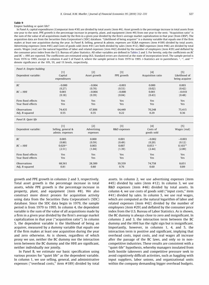
ARTICLE IN PRESS

Table 9Empire building or quiet life?

In Panel A, capital expenditures (Compustat item #30) are divided by total assets (item #6). Asset growth is the percentage increase in total assets from

one year to the next. PPE growth is the percentage increase in property, plant, and equipment (item #8) from one year to the next. ‘‘Acquisition ratio’’ is

the sum of the value of all acquisitions made by the firm in a given year divided by the firm’s average market capitalization in that year (from CRSP). The

acquisition data are from the Securities Data Corporation’s (SDC) database. ‘‘Likelihood of being acquirer’’ is a dummy variable that equals one if the firm

makes at least one acquisition during the year. In Panel B, Selling, general & admin. expenses are SG&A expenses (item #189) divided by total assets.

Advertising expenses (item #45) and Costs of goods sold (item #41) are both divided by sales (item #12). R&D expenses (item #46) are divided by total

assets. Wages (real) are the natural logarithm of labor and related expenses (item #42) divided by the number of employees (item #29) and deflated by

the consumer price index from the U.S. Bureau of Labor Statistics. All other variables are defined in Tables 2 and 3. For brevity, only the coefficients on BC

and BC � HHI are reported. The coefficients are estimated using OLS. Standard errors are clustered at the state of incorporation level. The sample period is

from 1976 to 1995, except in columns 4 and 5 of Panel A, where the sample period is from 1979 to 1995. t-Statistics are in parentheses. � , �� , and ��

denote significance at the 10%, 5%, and 1% levels, respectively.

Panel A: Empire building

[1] [2] [3] [4] [5]

Dependent variable: Capital Asset growth PPE growth Acquisition ratio Likelihood of

expenditures being acquirer

BC �0.000 �0.004 �0.003 0.000 0.003

(0.27) (0.70) (0.53) (0.02) (0.42)

BC � HHI 0.001 �0.004 �0.000 0.001 �0.010

(0.18) (0.39) (0.04) (0.43) (0.48)

Firm fixed effects Yes Yes Yes Yes Yes

Year fixed effects Yes Yes Yes Yes Yes

Observations 74,435 67,806 64,449 70,248 75,415

Adj. R-squared 0.55 0.35 0.22 0.29 0.36

Panel B: Quiet life

[1] [2] [3] [4] [5]

Dependent variable: Selling, general & Advertising R&D expenses Costs of Wages (real)

admin. expenses expenses goods sold

BC 0.005 0.000 0.001 �0.002 �0.003

(0.80) (0.59) (0.49) (0.20) (0.12)

BC � HHI 0.029�� 0.003 0.007 0.053 �� 0.103**

(2.51) (1.04) (1.39) (2.44) (2.00)

Firm fixed effects Yes Yes Yes Yes Yes

Year fixed effects Yes Yes Yes Yes Yes

Observations 68,561 28,389 39,359 74,758 8,651

Adj. R-squared 0.81 0.80 0.76 0.60 0.89


growth and PPE growth in columns 2 and 3, respectively.Total asset growth is the percentage increase in totalassets, while PPE growth is the percentage increase inproperty, plant, and equipment (item #8). We alsoconstruct more direct proxies for acquisition activityusing data from the Securities Data Corporation’s (SDC)database. Since the SDC data begin in 1979, the sampleperiod is from 1979 to 1995. In column 4, the dependentvariable is the sum of the value of all acquisitions made bya firm in a given year divided by the firm’s average marketcapitalization in that year (‘‘acquisition ratio’’). In column5, the dependent variable is the likelihood of being anacquirer, measured by a dummy variable that equals oneif the firm makes at least one acquisition during the yearand zero otherwise. As is shown, regardless of whichproxy we use, neither the BC dummy nor the interactionterm between the BC dummy and the HHI are significant,neither individually nor jointly.

In Panel B, we estimate our basic specification usingvarious proxies for ‘‘quiet life’’ as the dependent variable.In column 1, we use selling, general, and administrativeexpenses (‘‘overhead costs,’’ item #189) divided by total

assets. In column 2, we use advertising expenses (item#45) divided by sales (item #12). In column 3, we useR&D expenses (item #46) divided by total assets. Incolumn 4, we use costs of goods sold (‘‘input costs,’’ item#41) divided by sales. In column 5, we use real wages,which are computed as the natural logarithm of labor andrelated expenses (item #42) divided by the number ofemployees (item #29) and deflated by the consumer priceindex from the U.S. Bureau of Labor Statistics. As is shown,the BC dummy is always close to zero and insignificant. Incolumns 2 and 3, the interaction term between the BCdummy and the HHI has the right sign but is insignificant.Importantly, however, in columns 1, 4, and 5, theinteraction term is positive and significant, implying thatoverhead costs, input costs, and real wages all increaseafter the passage of the BC laws, and only so in non-competitive industries. These results are consistent with a‘‘quiet-life’’ hypothesis, whereby managers insulated fromboth hostile takeovers and competitive pressure seek toavoid cognitively difficult activities, such as haggling withinput suppliers, labor unions, and organizational unitswithin the company demanding bigger overhead budgets.

ARTICLE IN PRESS


Let us conclude with two caveats. First, the interactionterms in Panel B have smaller t-statistics than in ourregression in Table 3, presumably because the dependentvariables are all individual components of ROA. Thus,while the passage of the BC laws has a large andsignificant effect on ROA overall, it has only a relativelysmall effect on any individual component of ROA. Second,the wage result in Panel B should be taken with caution.Not only is the sample quite small, as only few firms inCompustat report wage data, but the data are also verynoisy (see Bertrand and Mullainathan, 1999). For instance,some firms report wage data only intermittently, whileothers report no wage data at all. What is more,Compustat only provides aggregate data on labor andrelated expenses, which also includes pension costs,payroll taxes, and employee benefits. On a positive note,our wage results are similar to those in Bertrand andMullainathan (1999, 2003), who report wage increasesbetween 1% and 2% after the passage of the BC laws.(In our case, the average wage increase is 1.9%.)

16 Choosing the estimation window adjacent to the first time

interval for which cumulative abnormal returns are computed (here:

the time interval ½�40;�2�) is common practice (MacKinlay, 1997).

However, we obtain similar results if we instead estimate the market

model for the time interval from 300 to 100 trading days prior to the

event date. We also obtain similar results if we use either a three- or

four-factor model instead of the market model.

5. Event-study results

Does the stock market anticipate that firms in compe-titive industries are largely unaffected by the passage of theBC laws? The main difficulty in answering this question liesin the choice of event date. Since the passage date itself iswell-anticipated, it is unlikely to contain much newinformation. Instead, one must find an early date at whichsignificant news about the law is disseminated to thepublic, e.g., the date of the first newspaper report about thelaw. For instance, Karpoff and Malatesta (1989), in theirevent study of anti-takeover laws, find no significantabnormal returns when using either the date of the law’sintroduction in the state legislature, its final passage, or itssigning by the governor as the event date. However, theydo find statistically significant abnormal returns whenusing the first date for which they could find a newspaperreport about the law as the event date.

Finding the first newspaper report about a BC law isoften a formidable task. Electronic archives of local news-papers often do not go back to the 1980s, while large out-of-state newspapers, such as the Wall Street Journal and theNew York Times, often provide no coverage, especially if thestate in question is small and only few firms areincorporated in it. After a careful search of major newspaperdatabases (ProQuest, Lexis-Nexis, Factiva, Newsbank Amer-ica’s Newspapers, Google News Archive), we could findnewspaper reports for 19 of the 30 BC laws in our sample:Arizona, Connecticut, Delaware, Georgia, Illinois, Kentucky,Maryland, Massachusetts, Minnesota, New Jersey, New York,Ohio, Oklahoma, Pennsylvania, South Carolina, Tennessee,Virginia, Washington, and Wisconsin. Most of the remaining11 states are small in terms of the number of incorporatedfirms. In fact, seven of them had fewer than 20 firms—andonly one (Nevada) had more than 100 firms—in the mergedCRSP-Compustat sample in the year in which the BC lawwas passed. The 19 states for which we could findnewspaper reports represent 92% of all firms incorporatedin states that passed a BC law during the sample period.

The event-study methodology is based on the assumptionthat the events are independent (MacKinlay, 1997). Whilethis assumption is satisfied in many applications, it is notsatisfied in our case. Since all firms incorporated in a givenstate are affected by the same event, their abnormal returnsare likely correlated, leading to biased standard errors. Acommon way to address this problem is to form portfoliosconsisting of all firms incorporated in a given state. Sincethe event dates are different for each state portfolio, the issueof cross-sectional correlation then becomes negligible(MacKinlay, 1997; Karpoff and Malatesta, 1989).

Our empirical methodology follows Karpoff andMalatesta (1989). For each state portfolio j, we estimatethe market model using CRSP daily return data from 241to 41 trading days prior to the event date.16 That is, weestimate

Rjt ¼ ajþbjRmtþejt ; ð3Þ

where Rjt is the daily return of the equally weightedportfolio of all firms incorporated in state j and Rmt is thedaily return of the equally weighted CRSP market portfolio.Substituting the estimates back into (3), we obtain anestimate of the normal portfolio return Rjt . The abnormalreturn of state portfolio j can then be computed as

ARjt :¼ Rjt � Rjt : ð4Þ

To obtain cumulative abnormal returns (CAR), we simplysum up the abnormal returns over the desired timeinterval. We report average CARs based on the 19 stateportfolios for the same time intervals as Karpoff andMalatesta (1989): ½�40;�2�, ½�3;�2�, ½�1;0�, [1,2], and[1,10], where ½�1;0� is the two-day event window. To seeif there is any systematic trend prior to the event date, weadditionally report average CARs for the time intervals½�30;�2�; ½�20;�2�, and ½�10;�2�.

The above methodology yields an estimate of theaverage impact of the BC laws on stock prices. To examineif the price impact is different for firms in competitive andnon-competitive industries, we divide each state portfoliointo equal-sized smaller portfolios. For each state j, weform a low- and high-HHI portfolio by sorting firms basedon whether their HHI lies below or above the median,respectively. We also do the same with low-, medium-, andhigh-HHI portfolios by sorting firms based on whethertheir HHI lies in the lowest, medium, and highest tercile,respectively. The remaining steps are the same as above.

The results are shown in Panel A of Table 10. As isshown in column 1, the average CAR in the two-day eventwindow is �0:32% (z-statistic of �2:58). Moreover, 14 ofthe 19 individual CARs are negative. Of equal interest is thatthe average two-day CARs immediately before and after thetwo-day event window are small and insignificant.

ARTICLE IN PRESS

Table 10Event-study results.

The methodology used to compute cumulative abnormal returns (CARs) is described in Section 5. The event date is the date of the first newspaper

report about the BC law. The two-day event window is denoted by ½�1;0�. The numbers reported in the table are average portfolio CARs based on 19 state

portfolios. The 19 states are Arizona, Connecticut, Delaware, Georgia, Illinois, Kentucky, Maryland, Massachusetts, Minnesota, New Jersey, New York,

Ohio, Oklahoma, Pennsylvania, Tennessee, South Carolina, Virginia, Washington, and Wisconsin. The construction of the state-HHI portfolios, bottom-HHI

portfolios, and top-HHI portfolios is described in Section 5. In Panel B, the hedge portfolio is long in the top-HHI portfolio and short in the bottom-HHI

portfolio. z-Statistics are in parentheses. � , �� , and �� denote significance at the 10%, 5%, and 1% levels, respectively.

Panel A: Event-study results

[1] [2] [3] [4] [5] [6]

All firms HHI ðLowÞ HHI ðHighÞ HHI ðLowÞ HHI ðMediumÞ HHI ðHighÞ

[�40,�2] 0.98 1.25 0.61 1.51 2.11 �0.30

(1.44) (1.40) (0.49) (1.53) (1.13) (0.04)

[�30,�2] 0.43 0.83 0.08 0.78 0.52 �0.34

(0.94) (1.08) (0.07) (1.02) (0.36) (0.07)

[�20,�2] 0.08 0.15 �0.01 0.33 �0.07 �0.41

(0.53) (0.47) (0.22) (0.78) (�0.03) (0.15)

[�10,�2] 0.52 0.44 0.57 0.44 1.15 0.10

(1.35) (1.31) (0.54) (1.19) (1.24) (0.21)

[�3,�2] �0.02 0.22 �0.24 0.38 0.09 �0.24

(0.05) (0.47) (�0.50) (0.75) (�0.26) (�0.25)

[�1,0] �0:32�� 0.10 �0:54�� 0.08 �0:44� �0:67��

(�2.58) (�1.29) (�2.36) (�0.53) (�1.67) (�2.31)

[1,2] 0.09 �0.03 0.20 0.01 0.25 0.03

(0.37) (0.07) (0.45) (�0.05) (1.02) (�0.28)

[1,10] �0.07 0.03 �0.17 0.30 �0.74 �0.27

(�0.08) (0.07) (�0.07) (0.78) (�0.53) (�0.61)

Panel B: Hedge portfolios

HHI Partition Median Terciles Quartiles Quintiles

Bottom-HHI portfolio �0.10 0.08 0.17 0.19

(�1.29) (�0.53) (�0.62) (�0.64)

Top-HHI portfolio �0.54 �� 0.67 �� 0.75 �� 0.78**

(�2.36) (�2.31) (�2.44) (�2.49)

Hedge portfolio 0.44 0.75 � 0.92 �� 0.97 ��

(1.41) (1.76) (2.02) (2.06)


Columns 2 and 3 show the average CARs for the low-and high-HHI portfolios. The average two-day event CARfor the low-HHI portfolio is small and insignificant, whilethe average two-day event CAR for the high-HHI portfoliois �0:54% (z-statistic of �2:36). Thus, while firms incompetitive industries experience no significant stockprice impact around the date of the first newspaper reportabout the BC law, firms in non-competitive industriesexperience a significant abnormal stock price decline.

Columns 4–6 show the average CARs for the low-,medium-, and high-HHI portfolios. The results are againsimilar. While firms in competitive industries experienceno significant stock price impact, firms in less competitiveindustries experience a significant abnormal stock pricedecline. Moreover, and consistent with the results incolumn 3 of Table 3, the stock price decline is monotonicin the HHI. While the average two-day event CAR for thelow-HHI portfolio is small and insignificant, the averagetwo-day event CARs for the medium- and high-HHIportfolios are �0:44% (z-statistic of �1:67) and �0:67%(z-statistic of �2:31), respectively.17

17 We obtain a similar monotonic pattern using median CARs. The

median two-day event CAR for the low-, medium-, and high-HHI

portfolio is 0:06%; �0:46%; and �0:67%; respectively. The corresponding

In Panel B, we test whether the average two-day eventCARs are significantly different between HHI groups. Foreach state j, we form a hedge portfolio that is long in thetop-HHI group and short in the bottom-HHI group, where‘‘top’’ and ‘‘bottom’’ are defined by the respective HHIpartition. Average CARs and z-statistics are computedbased on the 19 hedge portfolios. In column 1, we form ahedge portfolio that is long in the above-median HHIgroup and short in the below-median HHI group. As isshown, the average CARs of the two groups are notsignificantly different from each other (z-statistic of 1.41).This is not surprising. As is often the case with stockreturns, significant differences can only be found betweenextreme portfolios. In column 2, we form a hedgeportfolio that is long in the top-tercile HHI group andshort in the bottom-tercile HHI group. As is shown, thedifference between the two groups now becomes margin-ally significant (z-statistic of 1.76). If we consider evenfiner HHI partitions, this difference becomes even morepronounced. In columns 3 and 4, we form hedge portfoliosthat are based on HHI quartiles and quintiles, respectively.


ratio of positive to negative CARs in the two-day event window is 10:9,

4:15, and 5:14, respectively.

ARTICLE IN PRESS


In both cases, the difference between the bottom- andtop-HHI group is now significant at the 5% level(z-statistics of 2.02 and 2.06, respectively).

Let us conclude with a word of caution. To a certainextent, the event-study evidence alleviates concerns thatour main results are obtained using accounting variables,which can be manipulated (see Section 3.3). That said, itdoes not convey definitive evidence that firms in non-competitive industries experience a larger drop in profit-ability. It could be the case that, for a variety of reasons,the value gains from (hostile) takeovers are higher in non-competitive industries, in which case the larger stockprice decline in these industries might merely reflect thecapitalized value of higher forgone value gains.

6. Conclusion

Using the passage of business combination (BC) lawsas a source of exogenous variation, we examine if theselaws have a different effect on firms in competitiveand non-competitive industries. While firms in non-competitive industries experience a significant drop inoperating performance after the laws’ passage, firms incompetitive industries experience virtually no effect,which is consistent with the notion that competitionmitigates managerial slack. When we examine whichagency problem competition mitigates, we find evidencein support of a ‘‘ quiet-life’’ hypothesis. Input costs, wages,and overhead costs all increase after the laws’ passage,and only so in non-competitive industries. We obtain asimilar picture when conducting event studies around thedates of the first newspaper reports about the BC laws.While firms in non-competitive industries experience asignificant stock price decline, firms in competitiveindustries experience a small and insignificant stock priceimpact.

Our results have implications both for policy andresearch. For instance, our results suggest that policyefforts to improve corporate governance could benefitfrom focusing primarily on firms in non-competitiveindustries. Moreover, such efforts could be broadened toalso include measures aimed at improving an industry’scompetitiveness, such as deregulation and antitrust laws.Our results also suggest that researchers who want tostudy the effects of governance could benefit frominteracting governance proxies with measures of compe-tition. The empirical relationship might be stronger,both economically and statistically, for firms in non-competitive industries. To give an example, preliminaryfindings by the authors suggest that the positive alphagenerated by the governance hedge portfolio in Gompers,Ishii, and Metrick (2003) comes entirely from non-competitive industries (Giroud and Mueller, 2008b). Incontrast, the alpha in competitive industries is small andinsignificant. Hence, good governance at the firm level isassociated with higher equity prices in non-competitiveindustries, but not in competitive industries. While thesepreliminary findings are encouraging, more research isneeded before we can conclude that firm-level govern-ance instruments are moot in competitive industries.

References

Aggarwal, R., Samwick, A., 1999. Executive compensation, strategiccompetition, and relative performance evaluation: theory andevidence. Journal of Finance 54, 1999–2043.

Bertrand, M., Mullainathan, S., 1999. Is there discretion in wage setting?A test using takeover legislation. Rand Journal of Economics 30,535–554.

Bertrand, M., Mullainathan, S., 2003. Enjoying the quiet life? Corporategovernance and managerial preferences. Journal of Political Econo-my 111, 1043–1075.

Bertrand, M., Duflo, E., Mullainathan, S., 2004. How much should wetrust differences-in-differences estimates?. Quarterly Journal ofEconomics 119, 249–275.

Bloom, N., van Reenen, J., 2007. Measuring and explaining managementpractices across firms and countries. Quarterly Journal of Economics122, 1351–1408.

Carlton, D., Perloff, J., 1989. Modern Industrial Organization. Scott,Foresman Little, Brown, Glenview, IL.

Cheng, S., Nagar, V., Rajan, M., 2005. Identifying control motives inmanagerial ownership: evidence from antitakeover legislation. Re-view of Financial Studies 18, 637–672.

Comment, R., Schwert, W., 1995. Poison or placebo? Evidence on thedeterrence and wealth effects of modern antitakeover measures.Journal of Financial Economics 39, 3–43.

Cremers, M., Nair, V., Peyer, U., 2008. Takeover defenses and competi-tion: the role of stakeholders. Journal of Empirical Legal Studies 5,791–818.

Dechow, P., Sloan, R., Sweeney, A., 1995. Detecting earnings manage-ment. Accounting Review 70, 193–225.

Feenstra, R., 1996. U.S. imports, 1972–1994: data and concordances.NBER Working Paper 5515.

Feenstra, R., Romalis, J., Schott, P., 2002. U.S. imports, exports, and tariffdata, 1989–2001. NBER Working Paper 9387.

Garvey, G., Hanka, G., 1999. Capital structure and corporate control: theeffect of antitakeover statutes on firm leverage. Journal of Finance54, 519–546.

Giroud, X., Mueller, H., 2008a. Does corporate governance matter incompetitive industries? Unpublished Working Paper, New YorkUniversity.

Giroud, X., Mueller, H., 2008b. Corporate governance, product marketcompetition, and equity prices. Unpublished Working Paper, NewYork University.

Gompers, P., Ishii, J., Metrick, A., 2003. Corporate governance and equityprices. Quarterly Journal of Economics 118, 107–155.

Guadalupe, M., Perez-Gonzalez, F., 2005. The impact of product marketcompetition on private benefits of control. Unpublished WorkingPaper, Columbia University.

Hart, O., 1983. The market mechanism as an incentive scheme. BellJournal of Economics 14, 366–382.

Hermalin, B., 1992. The effects of competition on executive behavior.Rand Journal of Economics 23, 350–365.

Hicks, J., 1935. Annual survey of economic theory: the theory ofmonopoly. Econometrica 3, 1–20.

Holmstrom, B., Tirole, J., 1989. The theory of the firm. In: Schmalensee,R., Willig, R. (Eds.), Handbook of Industrial Organization. North-Holland, Amsterdam, pp. 61–133.

Hou, K., Robinson, D., 2006. Industry concentration and average stockreturns. Journal of Finance 61, 1927–1956.

Jones, J., 1991. Earnings management during import relief investigations.Journal of Accounting Research 29, 193–228.

Karpoff, J., Malatesta, P., 1989. The wealth effects of second-generationstate takeover legislation. Journal of Financial Economics 25,291–322.

Karuna, C., 2008. Industry product market competition and corporategovernance. Unpublished Working Paper, University of California atIrvine.

Lewellen, K., 2006. Financing decisions when managers are risk averse.Journal of Financial Economics 82, 551–589.

MacKinlay, A., 1997. Event studies in economics and finance. Journal ofEconomic Literature 35, 13–39.

Moulton, B., 1990. An illustration of a pitfall in estimating the effects ofaggregate variables on micro units. Review of Economics andStatistics 72, 334–338.

Nickell, S., 1996. Competition and corporate performance. Journal ofPolitical Economy 104, 724–746.

Odders-White, E., Ready, M., 2006. Credit ratings and stock liquidity.Review of Financial Studies 19, 119–157.

ARTICLE IN PRESS


Petersen, M., 2009. Estimating standard errors in finance panel data sets:comparing approaches. Review of Financial Studies 22, 435–480.

Rauh, J., 2006. Own company stock in defined contribution pension plans:A takeover defense?. Journal of Financial Economics 81, 379–410.

Romano, R., 1987. The political economy of takeover statutes. VirginiaLaw Review 73, 111–199.

Romano, R., 1993. Competition for corporate charters and the lesson oftakeover statutes. Fordham Law Review 61, 843–864.

Scharfstein, D., 1988. Product–market competition and managerial slack.Rand Journal of Economics 19, 147–155.

Scherer, F., 1980. Industrial Market Structure and Economic Perfor-mance. Rand McNally, Chicago, IL.

Schmidt, K., 1997. Managerial incentives and product market competi-tion. Review of Economic Studies 64, 191–213.

Shumway, T., 2001. Forecasting bankruptcy more accurately: a simplehazard model. Journal of Business 74, 101–124.

Smith, A., 1776. An inquiry into the nature and causes of the wealth ofnations. In: Cannan, E. (Ed.), Fifth Edition (1904). Methuen and Co.,Ltd., London.

Schwert, W., 2000. Hostility in takeovers: In the eyes of the beholder?.Journal of Finance 55, 2599–2640.

Teoh, S., Welch, T., Wong, T., 1998. Earnings management and the long-run market performance of initial public offerings. Journal of Finance53, 1935–1974.

Tirole, J., 1988. The Theory of Industrial Organization. MIT Press,Cambridge, MA.

Zhang, F., 2006. Information uncertainty and stock returns. Journal ofFinance 61, 105–136.

Journal of Financial Economics - New York Universitypeople.stern.nyu.edu/hmueller/papers/pmc.pdf ·...

Documents

Transcript of Journal of Financial Economics - New York Universitypeople.stern.nyu.edu/hmueller/papers/pmc.pdf ·...