Journal of Financial Economics - London Business Schoolfaculty.london.edu/aedmans/Rowe.pdf ·...
20
Does the stock market fully value intangibles? Employee satisfaction and equity prices $ Alex Edmans Wharton School, University of Pennsylvania, 3620 Locust Walk, Philadelphia, PA 19104, USA article info Article history: Received 31 December 2008 Received in revised form 28 January 2010 Accepted 31 December 2010 Available online 30 March 2011 JEL classification: G14 J28 M14 Keywords: Intangibles Market efficiency Underreaction Human capital Socially responsible investing abstract This paper analyzes the relationship between employee satisfaction and long-run stock returns. A value-weighted portfolio of the ‘‘100 Best Companies to Work For in America’’ earned an annual four-factor alpha of 3.5% from 1984 to 2009, and 2.1% above industry benchmarks. The results are robust to controls for firm characteristics, different weighting methodologies, and the removal of outliers. The Best Companies also exhibited significantly more positive earnings surprises and announcement returns. These findings have three main implications. First, consistent with human capital-centered theories of the firm, employee satisfaction is positively correlated with shareholder returns and need not represent managerial slack. Second, the stock market does not fully value intangibles, even when independently verified by a highly public survey on large firms. Third, certain socially responsible investing (SRI) screens may improve investment returns. & 2011 Elsevier B.V. All rights reserved. ‘‘[Costco’s] management is focused on y employees to the detriment of shareholders. To me, why would I want to buy a stock like that?’’—Equity analyst, quoted in BusinessWeek, 8/28/03 ‘‘I happen to believe that in order to reward the shareholder in the long term, you have to please your customers and workers.’’—Jim Sinegal, Costco’s CEO, quoted in the Wall Street Journal, 3/26/04 1. Introduction This paper analyzes the relationship between employee satisfaction and long-run stock returns. A value-weighted portfolio of the ‘‘100 Best Companies to Work For in America’’ (Levering, Moskowitz, and Katz, 1984; Levering and Moskowitz, 1993) earned a four-factor alpha of 0.29% per month from 1984 to 2009, or 3.5% per year. These figures exclude any event-study reaction to list inclusion and capture only long-run drift. When compared to industry-matched benchmarks, the alpha remains a statistically significant 2.1%. Contents lists available at ScienceDirect journal homepage: www.elsevier.com/locate/jfec Journal of Financial Economics 0304-405X/$ - see front matter & 2011 Elsevier B.V. All rights reserved. doi:10.1016/j.jfineco.2011.03.021 $ I thank an anonymous referee, Alon Brav, Henrik Cronqvist, Ingolf Dittmann, Florian Ederer, Xavier Gabaix, Rients Galema, Simon Gervais, Itay Goldstein, Adam Grant, David Hirshleifer, Tim Johnson, Mozaffar Khan, Lloyd Kurtz, Andrew Metrick, Milt Moskowitz, Stew Myers, Mahesh Pritamani, Luke Taylor, Jeff Wurgler, Yexiao Xu, David Yermack, and seminar participants at the China International Conference in Finance, FIRS, NYU Conference on Financial Economics and Accounting. Oxford Finance Symposium, Socially Responsible Investing annual con- ference, George Mason, MIT Sloan, National University of Singapore, Reading, Rockefeller, Rotterdam, UBS, Virginia Tech, Wharton, and York for valued input. Special thanks to Franklin Allen, Jack Bao, John Core and Rob Stambaugh for numerous helpful comments, and Amy Lyman of the Great Place To Work Institute for answering several questions about the Fortune survey. James Park provided superb research assistance, and Daniel Kim, Rob Ready and Patrick Sim assisted with data collection. I gratefully acknowledge support by the Goldman Sachs Research Fellow- ship from the Rodney White Center for Financial Research. E-mail address: [email protected] Journal of Financial Economics 101 (2011) 621–640
Transcript of Journal of Financial Economics - London Business Schoolfaculty.london.edu/aedmans/Rowe.pdf ·...

Contents lists available at ScienceDirect
Journal of Financial Economics
Journal of Financial Economics 101 (2011) 621–640
0304-40
doi:10.1
$ I th
Dittman
Itay Go
Khan, L
Mahesh
and se
Finance
Oxford
ference
Reading
for valu
Rob Sta
Great P
Fortune
Daniel
grateful
ship fro
E-m
journal homepage: www.elsevier.com/locate/jfec
Does the stock market fully value intangibles? Employee satisfactionand equity prices$
Alex Edmans
Wharton School, University of Pennsylvania, 3620 Locust Walk, Philadelphia, PA 19104, USA
a r t i c l e i n f o
Article history:
Received 31 December 2008
Received in revised form
28 January 2010
Accepted 31 December 2010Available online 30 March 2011
JEL classification:
G14
J28
M14
Keywords:
Intangibles
Market efficiency
Underreaction
Human capital
Socially responsible investing
5X/$ - see front matter & 2011 Elsevier B.V.
016/j.jfineco.2011.03.021
ank an anonymous referee, Alon Brav, Henr
n, Florian Ederer, Xavier Gabaix, Rients Gale
ldstein, Adam Grant, David Hirshleifer, Tim
loyd Kurtz, Andrew Metrick, Milt Mosko
Pritamani, Luke Taylor, Jeff Wurgler, Yexiao
minar participants at the China Internatio
, FIRS, NYU Conference on Financial Economi
Finance Symposium, Socially Responsible Inv
, George Mason, MIT Sloan, National Unive
, Rockefeller, Rotterdam, UBS, Virginia Tech,
ed input. Special thanks to Franklin Allen, Jack
mbaugh for numerous helpful comments, and
lace To Work Institute for answering several q
survey. James Park provided superb resear
Kim, Rob Ready and Patrick Sim assisted wit
ly acknowledge support by the Goldman Sach
m the Rodney White Center for Financial Res
ail address: [email protected]
a b s t r a c t
This paper analyzes the relationship between employee satisfaction and long-run stock
returns. A value-weighted portfolio of the ‘‘100 Best Companies to Work For in
America’’ earned an annual four-factor alpha of 3.5% from 1984 to 2009, and 2.1%
above industry benchmarks. The results are robust to controls for firm characteristics,
different weighting methodologies, and the removal of outliers. The Best Companies
also exhibited significantly more positive earnings surprises and announcement
returns. These findings have three main implications. First, consistent with human
capital-centered theories of the firm, employee satisfaction is positively correlated with
shareholder returns and need not represent managerial slack. Second, the stock market
does not fully value intangibles, even when independently verified by a highly public
survey on large firms. Third, certain socially responsible investing (SRI) screens may
improve investment returns.
& 2011 Elsevier B.V. All rights reserved.
‘‘[Costco’s] management is focused on y employees tothe detriment of shareholders. To me, why would I
All rights reserved.
ik Cronqvist, Ingolf
ma, Simon Gervais,
Johnson, Mozaffar
witz, Stew Myers,
Xu, David Yermack,
nal Conference in
cs and Accounting.
esting annual con-
rsity of Singapore,
Wharton, and York
Bao, John Core and
Amy Lyman of the
uestions about the
ch assistance, and
h data collection. I
s Research Fellow-
earch.
want to buy a stock like that?’’—Equity analyst, quotedin BusinessWeek, 8/28/03
‘‘I happen to believe that in order to reward theshareholder in the long term, you have to please yourcustomers and workers.’’—Jim Sinegal, Costco’s CEO,quoted in the Wall Street Journal, 3/26/04
1. Introduction
This paper analyzes the relationship between employeesatisfaction and long-run stock returns. A value-weightedportfolio of the ‘‘100 Best Companies to Work For in America’’(Levering, Moskowitz, and Katz, 1984; Levering andMoskowitz, 1993) earned a four-factor alpha of 0.29% permonth from 1984 to 2009, or 3.5% per year. These figuresexclude any event-study reaction to list inclusion and captureonly long-run drift. When compared to industry-matchedbenchmarks, the alpha remains a statistically significant 2.1%.
2 Faleye and Trahan (2006) find that the BCs exhibit superior con-
temporaneous accounting performance than peers over 1998–2004. Lau
and May (1998) find a similar link using the 1993 list, but Fulmer, Gerhart,
and Scott (2003) find no relationship. Filbeck and Preece (2003) show that
firms in the 1998 list exhibited higher returns prior to list inclusion. Simon
and DeVaro (2006) show that the BCs exhibit higher customer satisfaction.
A. Edmans / Journal of Financial Economics 101 (2011) 621–640622
The results are also robust to controlling for firm character-istics, different weighting methodologies, and adjusting foroutliers. The outperformance is at least as strong from 1998,even though the list was published in Fortune magazine andthus highly visible to investors. The Best Companies (BCs)exhibit significantly more positive earnings surprises andstock price reactions to earnings announcements: over thefour announcement dates in each year, they earn 1.2–1.7%more than peer firms. These findings contribute to threestrands of research: the increasing importance of humancapital in the modern corporation; the equity market’s failureto fully incorporate the value of intangible assets; and theeffect of socially responsible investing (SRI) screens oninvestment performance.
Existing theories yield conflicting predictions as towhether employee satisfaction is beneficial for firm value.Traditional theories (e.g., Taylor, 1911) are based on thecapital-intensive firm of the early 20th century, whichfocused on cost efficiency. Employees perform unskilledtasks and have no special status; just like other inputs suchas raw materials, management’s goal is to extract maximumoutput while minimizing their cost. Satisfaction arises ifemployees are overpaid or underworked, both of whichreduce firm value.1 Principal-agent theory also supports thiszero-sum view: the firm’s objective function is maximized byholding the worker to her reservation wage. In contrast,more recent theories argue that the role of employees hasdramatically changed over the past century. The currentenvironment emphasizes quality and innovation, for whichhuman, rather than physical, capital is particularly important(Zingales, 2000). Human relations theories (e.g., Maslow,1943; Hertzberg, 1959; McGregor, 1960) view employeesas key organizational assets, rather than expendable com-modities, who can create substantial value by inventing newproducts or building client relationships. These theoriesargue that satisfaction can improve retention and motivation,to the benefit of shareholders.
Which theory is borne out in reality is an importantquestion for both managers and investors, and providesthe first motivation for this paper. If the traditional viewstill holds today, managers should minimize expenditureon worker benefits, and investors should avoid firms thatfail to do so. In contrast to this view, and the existingevidence reviewed in Section 2.1, I find a strong, robust,positive correlation between satisfaction and shareholderreturns. This result provides empirical support for recenttheories of the firm focused on employees as the keyassets, e.g., Rajan and Zingales (1998), Carlin and Gervais(2009), and Berk, Stanton, and Zechner (2010).
I study long-run stock returns for three main reasons.First, they suffer fewer reverse causality issues than valua-tion ratios or profits. A positive correlation between
1 Indeed, agency problems may lead to managers tolerating insuffi-
cient effort and/or excessive pay, at shareholders’ expense. The manager
may derive private benefits from improving his colleagues’ compensa-
tion, such as more pleasant working relationships (Jensen and Meckling,
1976). Alternatively, high wages may constitute a takeover defense
(Pagano and Volpin, 2005). Cronqvist, Heyman, Nilsson, Svaleryd, and
Vlachos (2008) find that salaries are higher when managers are more
entrenched, which supports the view that high worker pay is inefficient.
valuation/profits and satisfaction could occur if performancecauses satisfaction, but a well-performing firm should notexhibit superior future returns as profits should already bein the current stock price, since they are tangible.2 Second,they are more directly linked to shareholder value thanprofits, capturing all the channels through which satisfac-tion may benefit shareholders and representing the returnsthey actually receive. In addition to profits, satisfaction maylead to many other tangible outcomes valued by the market,such as new products or contracts. Studying returns alsoallows for controls for risk.3 Third, valuation ratios or event-study returns may substantially underestimate any relation-ship, given ample previous evidence that the market fails tofully incorporate intangibles. Firms with high R&D (Lev andSougiannis, 1996; Chan, Lakonishok, and Sougiannis, 2001),advertising (Chan, Lakonishok, and Sougiannis, 2001), patentcitations (Deng, Lev, and Narin, 1999), and softwaredevelopment costs (Aboody and Lev, 1998) all earn superiorlong-run returns. The market may be even more likely toundervalue employee satisfaction since theory has ambig-uous predictions for whether it is desirable for firm value.
Indeed, investigating the market’s incorporation of satis-faction is my second goal. I aim not only to extend earlierresults to another category of intangibles, but also to shedlight on the causes of the non-incorporation documentedpreviously. The main explanation for prior results is thatintangibles are not incorporated because the market lacksinformation on their value (the ‘‘lack-of-information’’hypothesis). While R&D spending can be observed in anincome statement, this is an input measure uninformativeof its quality or success (Lev, 2004). Even if information isavailable on an output measure such as patent citations, themarket may ignore it if it is not salient (Deng et al.’s citationmeasure had to be hand-constructed) or about small firmswhich are not widely followed (Hong, Lim, and Stein, 2000).
This paper evaluates the above hypothesis by using aquite different measure of intangibles to prior research,which addresses investors’ lack of information. The BC listmeasures satisfaction (an output) rather than expenditureon employee-friendly programs (an input). It is also parti-cularly visible: from 1998 it has been widely disseminatedby Fortune, and it covers large companies (median marketvalue of $5bn in 1998). Moreover, it is released on a specificevent date which attracts widespread attention, because itdiscloses information on several companies simultaneously.4
These results are consistent with reverse causality from performance to
satisfaction, and do not have implications for the market’s valuation of
intangibles or the profitability of an SRI trading strategy.3 Goenner (2008) controls for the market beta but not other factors
or characteristics.4 By contrast, R&D is one of many measures reported in a company’s
earnings announcement, and such announcements occur at different times
for different firms. Gompers, Ishii, and Metrick (2003), Yermack (2006), and
Liu and Yermack (2007) also document long-run abnormal returns. Their
measures of corporate governance, corporate jets, and CEO mansions are
also not released on a specific date and widely disseminated.

A. Edmans / Journal of Financial Economics 101 (2011) 621–640 623
If lack of information is the primary reason for previous non-incorporation findings, there should be no excess returns tothe BC list.
My analysis is a joint test of satisfaction both benefit-ing firm value and not being fully valued by the market.By delaying portfolio formation until the month after listpublication, I give the market ample opportunity to reactto its content. Yet, I still find significant outperformance.This result suggests that the non-incorporation of intan-gibles found by prior research does not stem purely fromlack of information, but other factors. Even if investorswere aware of firms’ levels of satisfaction, they may havebeen unaware of its benefits, since theory providesambiguous predictions. An alternative explanation is thatinvestors use traditional valuation methodologies,devised for the 20th century firm and based on physicalassets, which cannot incorporate intangibles easily. Theresults also support managerial myopia theories (e.g.,Stein, 1988; Edmans, 2009), in which managers under-invest in intangible assets because they are invisible tooutsiders and thus do not improve the stock price. Even ifmanagers are able to provide information on the value oftheir intangibles (e.g., by hiring independent firms toaudit their value), the market may not capitalize them.
In addition to the valuation of intangibles, the papercontributes to the broader literature on market under-reaction since the Fortune study has a clearly definedrelease date, in contrast to previous intangible measures.Prior research finds that underreaction is strongest forsmall firms (e.g., Hong, Lim, and Stein, 2000); moregenerally, Fama and French (2008) find that most anoma-lies are confined to small stocks and thus hard to exploitgiven their high transactions costs. Here, underreactionoccurs even though most firms in the BC list are large, andso the mispricing is exploitable.
The third implication relates to the profitability of SRIstrategies, whereby investors only select companies thathave a positive impact on stakeholders other than share-holders. Employee welfare is an SRI screen used by a numberof funds. Traditional portfolio theory (e.g., Markowitz, 1959)suggests that any SRI screen reduces returns, since it restrictsan investor’s choice set; mathematically, a constrainedoptimization is never better than an unconstrained optimi-zation. Indeed, many existing studies find a zero (Hamilton,Jo, and Statman, 1993; Kurtz and DiBartolomeo, 1996;Guerard, 1997; Bauer, Koedijk, and Otten, 2005; Schroder,2007; Statman and Glushkov, 2008) or negative (Geczy,Stambaugh, and Levin, 2005; Brammer, Brooks, and Pavelin,2006; Renneboog, Ter Horst, and Zhang, 2008; Hong andKacperczyk, 2009) effect of SRI screens. While Moskowitz(1972), Luck and Pilotte (1993), and Derwall, Guenster,Bauer, and Koedijk (2005) find certain SRI screens improvereturns, these results are based on short time periods.
The Markowitz (1959) argument suggests that any SRIscreen worsens performance, and so it is sufficient touncover one screen that improves performance to contra-dict it. I study a screen based on employee satisfaction asthere is a strong theoretical motivation for why it mayexhibit a positive correlation with stock returns (seeSection 2). Indeed, I find an SRI screen that can improvereturns. If an investor is aware of every asset in the
economy, an SRI screen can never help, as non-SRI investorsare free to choose the screened stocks anyway. However, ifshe can only learn about a subset of the available universedue to time constraints (as in Merton, 1987), the SRI screen– rather than excluding good investments – may focus thechoice set on good investments. A firm’s concern for otherstakeholders, such as employees, may ultimately benefitshareholders (the first implication of the paper), yet not bepriced by the market as ‘‘stakeholder capital’’ is intangible(the second implication).
There are several potential explanations for the positivereturns found in this paper. One is mispricing: high satisfac-tion causes higher firm value, as predicted by human capitaltheories, but the market fails to capitalize it immediately.Indeed, both the magnitude and duration of the excessreturns are similar to or lower than found by analyses oflong-run returns to other intangibles, firm characteristics, orcorporate events. Thus, the mispricing implied by thisexplanation is within the bounds of what prior literaturehas found to be feasible. Under a mispricing channel, an
intangible only affects the stock price when it subsequently
manifests in tangible outcomes that are valued by the market.I indeed find that the BCs have significantly more positiveearnings surprises than peer firms and greater abnormalreturns to earnings announcements. A mispricing story alsoimplies that the BCs’ outperformance might not be perma-nent, for two reasons. First, some firms are only on the listfor a finite period: employee satisfaction may vary withchanges in management or a firm’s human resource policy(perhaps as a result of financial constraints). Thus, the levelof intangibles and hence mispricing fall over time. Second,even for firms for which satisfaction is reasonably perma-nent, the market may learn about its true value over time asit releases positive tangible news. Consistent with bothchannels, I find the drift to list inclusion declines over timeand becomes insignificant in the fifth year. In contrast, priorstudies of mergers and acquisitions (M&A) (Agrawal, Jaffe,and Mandelker, 1992; Loughran and Vijh, 1997), valuestrategies (Lakonishok, Shleifer, and Vishny, 1994), andequity issuance (Spiess and Affleck-Graves, 1995; Loughranand Ritter, 1995) find no evidence of returns declining in thefifth year, and so the above explanation requires less mis-pricing than these earlier findings. Consistent with thesecond channel in particular, the returns sharply decline inthe fifth year even for firms that remain on the list for all fiveyears. Consistent with the first channel in particular, buyingstocks dropped from the BC list or not updating the portfoliofor future lists leads to lower returns than holding the mostcurrent list.
An alternative causal interpretation is that superiorreturns are caused not by employee satisfaction, but listinclusion per se—it encourages SRI funds to buy the BCs,and this demand caused their prices to rise. I find that SRIfunds that use labor or employment screens increased theirweighting on the BCs over time, but this effect can explainat most 0.02% of the annual outperformance. Moreover, aswith other long-run event studies (e.g., Gompers, Ishii, andMetrick, 2003; Yermack, 2006; Liu and Yermack, 2007), wedo not have a natural experiment with random assignmentof the variable of interest to firms, and so the data admitnon-causal explanations. First, the use of long-run stock

5 These theories imply a high level of compensation, but do not
suggest that the form of compensation should be in satisfaction com-
pared to cash. Indeed, in the early 20th century, cash was viewed as the
most effective motivator: given harsh economic conditions, workers
were mainly concerned with physical needs such as food and shelter,
which could be addressed with money. Such a view would motivate a
study of wages rather than satisfaction. Again, human relations theories
stress that the world is different nowadays. Maslow (1943) and
Hertzberg (1959) argue that money is only an effective motivator up
to a point: once workers’ physical needs are met, they are motivated by
non-pecuniary factors such as job satisfaction, which cannot be exter-
nally purchased with cash and can only be provided by the firm. Hence,
satisfaction is an efficient form of compensation.
A. Edmans / Journal of Financial Economics 101 (2011) 621–640624
returns only reduces, rather than eliminates, reverse caus-ality concerns. While publicly observed profits shouldalready be in the current stock price, reverse causality canoccur in the presence of private information; employeeswith favorable information report higher satisfaction today,and the market is unaware that the list conveys suchinformation. This explanation is unlikely given the seven-month time lag between responding to the BC survey andthe start of the return compounding window; in addition,existing studies suggest that workers have no superiorinformation on their firm’s future returns (e.g., Benartzi,2001; Bergman and Jenter, 2007). Second, satisfaction mayproxy for other variables that are positively linked to stockreturns and also misvalued by the market. While I controlfor an extensive set of observable characteristics and covar-iances, by their very nature unobservables (such as goodmanagement) cannot be directly controlled for. If eitherreverse causality or omitted variables account for the bulkof the results, improving employee welfare may not causeincreases in shareholder value. However, the second andthird conclusions of the paper still remain: the existence of aprofitable SRI trading strategy on large firms, and themarket’s failure to incorporate the contents of a highly visiblemeasure of intangibles—regardless of whether the list cap-tures satisfaction, management, or employee confidence.
This paper is organized as follows. Section 2 discussesthe theoretical motivation for hypothesizing a link betweenemployee satisfaction and stock returns. Section 3 discussesthe data and methodology and Section 4 presents theresults. Section 5 discusses the possible explanations forthe findings and Section 6 concludes.
2. Theoretical motivation: Why might employeesatisfaction lead to excess returns?
For employee satisfaction to lead to superior returns,this requires that employee satisfaction is both beneficialfor firm value and not immediately capitalized by themarket. Sections 2.1 and 2.2 provide the motivation foreach hypothesis.
2.1. Employee satisfaction and firm value
It may seem intuitive that employee satisfaction shouldimprove firm performance, perhaps even removing the needto demonstrate such a relationship empirically. However,the traditional theories reviewed in the introduction suggestthe opposite relationship, and existing evidence finds littlesupport for the human relations view. Abowd (1989) showsthat announcements of pay increases reduce market valua-tions dollar-for-dollar; Diltz (1995) finds stock returns areuncorrelated with the Council of Economic Priorities (CEP)minority management and women in management vari-ables, and negatively correlated with family benefits;Dhrymes (1998) finds no relationship with KLD’s employeerelations variable; and Gorton and Schmid (2004) show thatgreater employee involvement reduces profitability andvaluation. On the one hand, such research renders therelationship non-obvious, and thus interesting to study. Onthe other hand, it is necessary to have a convincing a priorihypothesis for why a positive link might exist in spite of the
above research, to mitigate ‘‘data-mining’’ concerns and therisk that any correlation is spurious rather than reflecting atrue economic relationship.
Human relations theories argue that satisfaction maybenefit shareholders through two mechanisms. The first ismotivation. In traditional manufacturing firms, motivationwas simple because workers’ output could be easily mea-sured, allowing the use of monetary ‘‘piece rates’’ (Taylor,1911). In the modern firm, workers’ tasks are increasinglydifficult to quantify, such as building client relationships.Output-based incentives may thus be ineffective or evendestructive (Kohn, 1993). The reduced effectiveness ofextrinsic motivators increases the role for intrinsic motiva-tors such as satisfaction. This role is microfounded in botheconomics and sociology. The efficiency wage theory ofAkerlof and Yellen (1986) argues that ‘‘excess’’ satisfactioncan increase effort, because the worker wishes to avoidbeing fired from a satisfying job (Shapiro and Stiglitz, 1984)or views it as a ‘‘gift’’ from the firm and responds witha ‘‘gift’’ of increased effort (Akerlof, 1982). Sociologicaltheories argue that satisfied employees identify with thefirm and internalize its objectives, thus inducing effort(McGregor, 1960). A second channel is retention. In thetraditional firm, retention was unimportant as employeesperformed unskilled tasks. In contrast, they are the keysource of value creation in modern knowledge-based indus-tries, such as pharmaceuticals or software. Relatedly, highsatisfaction can be a valuable recruitment tool.5 A quiteseparate benefit to those predicted by human relationstheories is that customers may be more willing to patronizefirms which treat their workers fairly—for example, WholeFoods actively advertises its list inclusion to customers.
2.2. Underpricing of employee satisfaction
In an efficient market, a tangible variable that isunambiguously beneficial to firm value will be rapidlycapitalized and not lead to excess returns. However, abroad strand of existing research demonstrates under-pricing of a number of firm characteristics. Starting withstudies of intangibles in particular, Lev and Sougiannis(1996) find a 4.6% abnormal return based on R&D capital,and Chan, Lakonishok, and Sougiannis (2001) show thatfirms in the top quintile of R&D flows earn excess returnsof 6.1%. Advertising (Chan, Lakonishok, and Sougiannis,2001), patent citations (Deng, Lev, and Narin, 1999), andsoftware developments (Aboody and Lev, 1998) are alsoassociated with excess returns. Moving to other variables,

7 While the Institute was not founded until 1990, Levering and
Moskowitz used the same criteria for the 1984 list, although they
surveyed employees directly rather than through a questionnaire.8 After evaluations are completed, if significant negative news
A. Edmans / Journal of Financial Economics 101 (2011) 621–640 625
Gompers, Ishii, and Metrick (2003) find 8.5% abnormalreturns to a governance portfolio, Yermack (2006) docu-ments a negative 3.8% alpha to firms in which the CEOuses a corporate jet, Liu and Yermack (2007) show 13.8%returns to a portfolio formed on CEO homes, and Hongand Kacperczyk (2009) find a 3.2% alpha to sin stocks.
This paper is also related to studies of long-run drift,since the BC list has a clearly defined release date.Numerous studies find large and persistent drift after avariety of corporate events. For M&A, Agrawal, Jaffe, andMandelker (1992) find that acquirers suffer �10% abnor-mal returns over the next five years; Loughran and Vijh(1997) show that cash tender offers (stock mergers)outperform their benchmarks by 62% (�25%) over afive-year period. Both find that abnormal returns are stillstrong in the fifth year. For initial public offerings (IPOs),Ritter (1991) finds underperformance of 29.1% over threeyears and that the underperformance is still strong in yearthree; Loughran (1993) documents �45% returns overfive years which only die out in year six. For seasonedequity offerings (SEOs), Spiess and Affleck-Graves (1995)show underperformance of 31–39% over five years;Loughran and Ritter (1995) consider IPOs and SEOstogether and find �30% returns over five years. Neitherfind that returns abate even in year five. Michaely, Thaler,and Womack (1995) discover returns to dividend initia-tions (omissions) of 25% (�15%) over three years and onlyevidence of the omission drift declining in the third year.Lakonsihok and Vermaelen (1990) find 17% abnormalreturns to repurchase tender offers over two years with noevidence of the returns dying out; Ikenberry, Lakonishok,and Vermaelen (1995) find 12% returns to open-marketrepurchases (45% for value stocks) over four years, withreturns only abating in the final year. Moving away fromevent studies but to other analyses of long-run returns,Lakonishok, Shleifer, and Vishny (1994) find that a value-growth portfolio earns 10% per year and that the returns arestronger in the fifth year than all other years.
In addition to providing evidence for both mispricingand long-horizon drift, existing research also providesguidelines on the magnitude and duration of excessreturns that are plausible. Most closely related are theother intangibles studies which suggest abnormal returnsof up to 4–6% per year are possible. Some of the otherstudies find even greater annual excess returns.6 Movingto the duration of the drift, the studies of M&A, IPOs, andSEOs find no evidence of abnormal returns abating even inthe fifth year. Moreover, the bounds of plausibility for themagnitude and longevity of underpricing of employeesatisfaction may be even greater, for two reasons. First,satisfaction is an intangible, while many of the otherstudies investigate tangible characteristics and eventswhich are easier to incorporate into traditional valuationmethodologies. Second, theory offers reasonably clearpredictions for the direction of the effect of many pre-viously studied events on firm value. For example,
6 The alphas of Lakonishok, Shleifer, and Vishny (1994), Gompers,
Ishii, and Metrick (2003), and Liu and Yermack (2007) should be halved
for comparison with the present setting as they study long-short
portfolios.
signaling and free cash flow theories predict that dividendinitiations and repurchases should increase firm value,and equity issuance and dividend omissions shouldreduce it; despite these clear predictions, there is stillsignificant drift. As previously discussed, traditional the-ories and existing evidence suggest that employee satis-faction is negatively correlated with firm value. Thus,even if the changing nature of the firm suggests therelationship may now be positive, the persistence of thetraditional view may mean the market does not capitalize it.
The majority of the above studies find long-horizondrift, but do not identify the mechanism. However, somepapers provide evidence that one channel through whichfirm characteristics generate superior returns is that theylead to future tangible outcomes that are valued by themarket. La Porta, Lakonishok, Shleifer, and Vishny (1997)find that value stocks exhibit superior earnings surprisesto glamour stocks, and Giroud and Mueller (2011) find thesame for well-governed firms in non-competitive industriescompared to their worse-governed peers. Masulis, Wang,and Xie (2007) find that better-governed firms experiencesuperior returns to M&A announcements.
3. Data and summary statistics
My main data source is the list of the ‘‘100 BestCompanies to Work for in America.’’ This list was firstpublished in a book in March 1984 (Levering, Moskowitz,and Katz, 1984) and updated in February 1993 (Leveringand Moskowitz, 1993). Since 1998, it has been featured inFortune magazine each January. The list has been headedby Robert Levering and Milt Moskowitz throughout its26-year existence. It is compiled from two principalsources. Two-thirds of the score comes from employeeresponses to a 57-question survey created by the GreatPlace to Works Institute in San Francisco.7 This surveycovers topics such as attitudes toward management, jobsatisfaction, fairness, and camaraderie. Across all levels ofemployees, 250 are randomly selected in each firm, fill inthe surveys anonymously, and return their responsesdirectly to the Institute. The response rate is around60%. The remaining one-third of the score comes fromthe Institute’s evaluation of factors such as a company’sdemographic makeup, pay and benefits programs, andculture. The companies are scored in four areas: cred-ibility (communication to employees), respect (opportu-nities and benefits), fairness (compensation, diversity),and pride/camaraderie (teamwork, philanthropy, celebra-tions).8 Importantly, Fortune has no involvement in thecompany evaluation process, else it may have incentives
comes to light that may significantly damage employees’ faith in
management, the Institute may exclude that company from the list.
Only news that damages employee trust is relevant-a decline in profits is
not an example of such news, unless it has been caused by (say)
unethical behavior. Ever since list commencement, fewer than five firms
have been excluded for this reason.
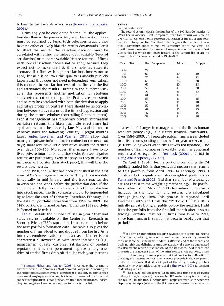
Table 1Summary statistics.
The second column details the number of the 100 Best Companies to
Work For in America (Best Companies) that had returns available on
CRSP for at least one month between publication of the list of that year,
and the subsequent list. The third column gives the number of new
public companies added to the Best Companies list of that year. The
fourth column contains the number of companies on the previous Best
Companies list which no longer feature in the current list or are no
longer public. The sample period is 1984–2009.
Year of list Best Companies Added Dropped
1984 78
1993 69 30 39
1998 70 34 33
1999 68 26 28
2000 60 20 28
2001 55 15 20
2002 55 13 13
2003 61 14 8
2004 57 11 15
2005 58 11 10
2006 50 8 16
2007 47 10 13
2008 42 11 16
2009 39 7 10
10 If a firm de-lists and the delisting payment date is prior to the end
of the month, delisting returns are used where the monthly return is
missing. If the delisting payment date is after the end of the month and
both monthly and delisting returns are available, the two are aggregated
to calculate the return of the month. At the start of the next month, the
proceeds are reinvested in all of the other stocks in the portfolio, based
on their relative weights in the portfolio at that point in time. Results are
A. Edmans / Journal of Financial Economics 101 (2011) 621–640626
to bias the list towards advertisers (Reuter and Zitzewitz,2006).9
Firms apply to be considered for the list; the applica-tion deadline is the previous May and the questionnairesmust be returned by June. Such selection issues eitherhave no effect or likely bias the results downwards. For itto affect the results, the selection decision must becorrelated with either the independent variable (level ofsatisfaction) or outcome variable (future returns). If firmswith low satisfaction choose not to apply because theyexpect not to make the list, this simply increases itsaccuracy. If a firm with high satisfaction chooses not toapply because it believes this quality is already publiclyknown and thus does not need independent verification,this reduces the satisfaction level of the firms in the listand attenuates the results. Turning to the outcome vari-able, this represents another motivation for studyingstock returns rather than profits. Profits are persistent,and so may be correlated with both the decision to applyand future profits. In contrast, there should be no correla-tion between stock returns at the time of application andduring the return window (controlling for momentum).Even if management has temporary private informationon future returns, this likely has little effect since listapplications must be made by late May and the returnwindow starts the following February 1 (eight monthslater). Jenter, Lewellen, and Warner (2011) show thatmanagers’ private information is confined to the next 100days; managers have little predictive ability for returnsover days 100–150. Moreover, if managers have long-lived private information and those who foresee negativereturns are particularly likely to apply (as they believe listinclusion will bolster their stock price), this will bias theresults downwards.
Since 1998, the BC list has been published in the firstissue of Fortune magazine each year. The publication dateis typically in mid-January, and the issue reaches thenewsstands one week before the publication date. If thestock market fully incorporates any effect of satisfactioninto stock prices, the list contents should be impoundedby at least the start of February. Therefore, February 1 isthe date for portfolio formation from 1998 to 2009. The1984 portfolio is formed on April 1, and the 1993 portfoliois formed on March 1.
Table 1 details the number of BCs in year t that hadstock returns available on the Center for Research inSecurity Prices (CRSP) tapes in at least one month beforethe next portfolio formation date. The table also gives thenumber of firms added to and dropped from the list. As isintuitive, employee satisfaction is a reasonably persistentcharacteristic. However, as with other intangibles (e.g.,management quality, customer satisfaction, or productreputation), it is not permanent—approximately one-third of traded firms drop off the list each year, perhaps
9 Statman, Fisher, and Anginer (2008) investigate the returns to
another Fortune list, ‘‘America’s Most Admired Companies,’’ focusing on
the ‘‘long-term investment value’’ component of this list. This list is not a
measure of employee satisfaction, but investors’ views of the firms and
so their interpretation is that it measures irrational exuberance. Indeed,
they find negative long-horizon returns to firms in this list.
as a result of changes in management or the firm’s humanresource policy (e.g., if it suffers financial constraints).Over 1984–2009, 244 separate public firms were includedin a list, corresponding to 1,616 firm-year observations(810 excluding years when the list was not updated). Thenumber of firms compares favorably to similar abnormalreturn studies, e.g., 104 in Yermack (2006) and 193 inHong and Kacperczyk (2009).
On April 1, 1984, I form a portfolio containing the 74publicly traded BCs in that year, and measure the returnsto this portfolio from April 1984 to February 1993. Iconstruct both equal- and value-weighted portfolios asFama and French (2008) find that a number of anomaliesare not robust to the weighting methodology. The portfo-lio is reformed on March 1, 1993 to contain the 65 firmsincluded in the new list, and returns are calculatedthrough January 1998. This process is repeated untilDecember 2009 and I call this ‘‘Portfolio I.’’10 If a BC isinitially private but goes public before the next list, I addit to the portfolio from the first full month after it startstrading. Portfolio I features 78 firms from 1984 to 1993,since four firms in the initial list became public over thatperiod.11
unchanged if I instead reinvest any takeover proceeds in the new parent,
under the rationale that at least part of the merged entity exhibits
superior employee satisfaction, or use the Shumway (1997) adjustment
to delisting returns.11 The results are unchanged when excluding firms that go public
midway through the year (to ensure that IPO underpricing is not driving
the results). In addition, I include Best Companies with only American
Depository Receipts (ADRs) in the U.S., since an investor constrained to

Table 2Summary characteristics.
Summary characteristics for the 74 companies in the 1984 ‘‘100 Best Companies to Work For in America’’ (Levering, Moskowitz, and Katz, 1984) list
that were public on April 1, 1984, and the 69 companies in the 1998 list published in Fortune that were public on February 1, 1998. The first two items are
taken from CRSP at the end of March 1984 (January 1998, respectively.) The last three items are based on CRSP and Compustat data for 1997 (1983),
missing for companies that were not traded in 1997 (1983), and excluded for companies for which only the ADRs are traded.
# obs Mean Median Std. dev. Min Max
1984 List
Market Cap ($ bn) 74 3.99 1.25 9.48 0 69.47
Price ($) 74 37.43 33.88 19.64 5.91 113.75
Dividend yield (%) 69 2.45 2.23 2.03 0 9.06
Market/book 69 2.41 1.95 1.82 0.68 10.80
Intangibles as a % of total assets (%) 69 0.91 0 2.15 0 10.35
1998 List
Market Cap ($ bn) 69 21.33 5.24 39.52 0.03 204.59
Price ($) 69 51.35 44.22 25.47 5.38 127.56
Dividend yield (%) 63 1.60 1.03 4.31 0 34.26
Market/book 63 5.20 4.13 4.22 �5.34 20.91
Intangibles as a % of total assets (%) 63 5.23 0.08 7.75 0 29.97
A. Edmans / Journal of Financial Economics 101 (2011) 621–640 627
Table 2 presents summary statistics on the original 74BCs in March 1984, and the 69 BCs in the first Fortune listin January 1998. Most notably, the firms are large, with amean (median) market value of $4bn ($1bn) in 1984 and$21bn ($5bn) in 1998. As a comparison, the 80th percen-tile breakpoint for the Fama-French size portfolios was$1bn in 1984 and $4bn in 1998. The average market-bookratio is a high 2.4 in 1984 (5.2 in 1998) and the mean ratioof intangibles to total assets is only 0.9% (5.2%). Together,these results suggest that these companies have littlehuman capital on the balance sheet, possibly becauseaccounting standards hinder capitalization, increasing thelikelihood that it is not fully valued. The most commonindustries in 1984 were consumer goods (seven compa-nies), hardware (7), measuring and control equipment (5),retail (5), and financial services (5). In 1998 they wereconsumer goods (7), financial services (6), software (5),pharmaceuticals (5), hardware (4), and electronic equip-ment (4). Human capital is plausibly an important inputin nearly all of these industries, with the link perhaps lessobvious for consumer goods.
Other measures of employee satisfaction and intangibleshave been studied in the literature, but the use of the BestCompanies list is superior for all three goals of the paper. Forthe first goal, studying the effect of satisfaction on firmvalue is challenging because it is very difficult to measure.The previously used measures of CEP and KLD are lessinformative as they are only based on observable practices,such as minority representation. They are easier tomanipulate—a firm that cares little for employee welfaremay hire a minority director to ‘‘check the box.’’ Suchmeasurement error may explain the insignificant previousfindings. The BC list is arguably the most thorough measureavailable, receiving significant attention from shareholders,management, employees, and the media. As outlined above,in addition to considering observable practices, it involves
(footnote continued)
hold U.S. shares would have been able to invest in such firms. The results
are unchanged when excluding firms with ADRs.
an in-depth ‘‘grass-roots’’ analysis through extensively sur-veying the workers. It is also available for 26 years, whereasother measures exist for shorter periods and thus the resultsmay lack power or be driven by outliers. (Naturally, studyingother intangibles such as R&D would not assess humancapital theories.) Second, the BC list is useful for studyingthe market’s incorporation of intangibles since it is highlypublic and attracts substantial attention given its perceivedaccuracy. It is therefore more salient than not only othersatisfaction measures but also other intangibles studied byprior literature, and allows testing of the ‘‘lack-of-informa-tion’’ hypothesis. The list also has a clearly defined releasedate, allowing underreaction and drift to be tested. For thepaper’s third goal, the list is publicly available and easilytradable by an SRI investor. Studying other intangibles wouldhave no implications for SRI, since intangibles such as R&Dand advertising are not SRI screens. In sum, the list appearsunique in being both a thorough measure of employeesatisfaction (allowing testing of human relations theoriesand SRI) and highly public (allowing testing of the marketvaluation of intangibles and returns available to investors).
4. Analysis and results
To ensure that any outperformance of the BCs does notresult from risk, I control for the four Carhart (1997)factors using
Rt ¼ aþbMKT MKTtþbHMLHMLtþbSMBSMBtþbMOMMOMtþeit ,
ð1Þ
where Rit is the return on Portfolio I in month t in excess of abenchmark, described below. a is an intercept that capturesthe abnormal risk-adjusted return. MKTt, HMLt, SMBt, andMOMt are the returns on the market, value, size, andmomentum factors, taken from Ken French’s Web site.
Standard errors are calculated using Newey and West(1987), which allows for eit to be heteroskedastic andserially correlated. The returns Rit are calculated overthree different benchmarks. The first is the risk-free ratefrom Ibbotson Associates. The second is an industry-matched portfolio using the 49-industry classification of

Table 3Risk-adjusted returns.
Monthly regressions of returns to a portfolio of the ‘‘100 Best
Companies to Work For in America’’ on the four Carhart (1997) factors,
MKT, HML, SMB, and MOM. The dependent variable is the portfolio return
less either the risk-free rate, the industry-matched portfolio return, or
the characteristics-matched portfolio return. Panel A contains equal-
weighted returns and Panel B contains value-weighted returns. The
alpha is the excess risk-adjusted return. t-Statistics are in parentheses.
The sample period is April 1984–December 2009.
Excess returns over
Risk-free Industry Characteristics
Panel A: Equal-weighted
a 0.31 0.20 0.24
(3.34)nnn (2.76)nnn (2.94)nnn
bMKT 1.08 0.06 0.09
(41.01)nnn (3.55)nnn (3.69)nnn
bHML 0.03 0.09 0.01
(0.70) (3.22)nnn (0.45)
bSMB 0.17 0.15 0.05
(3.66)nnn (5.70)nnn (1.39)
bMOM �0.15 �0.07 �0.09
(�6.36)nnn (�3.39)nnn (�4.80)nnn
Panel B: Value-weighted
a 0.29 0.17 0.15
(2.59)nnn (2.28)nn (2.15)nn
bMKT 1.00 �0.04 0.01
(35.68)nnn (�0.18) (0.59)
bHML �0.37 �0.03 �0.11
(�7.64)nnn (�0.76) (�3.32)nnn
bSMB �0.17 �0.21 �0.03
(�3.64)nnn (�6.63)nnn (�0.88)
bMOM �0.06 �0.02 �0.04
(�1.78)n (�0.81) (�2.11)nn
# obs 309 309 309
n: Significant at the 10% level; nn: Significant at the 5% level; nnn:
Significant at the 1% level.
Table 4Risk-adjusted returns from 1998.
Monthly regressions of returns to a portfolio of the ‘‘100 Best
Companies to Work For in America’’ on the four Carhart (1997) factors,
MKT, HML, SMB, and MOM. The dependent variable is the portfolio return
less either the risk-free rate, the industry-matched portfolio return, or
the characteristics-matched portfolio return. Panel A contains equal-
weighted returns and Panel B contains value-weighted returns. The
alpha is the excess risk-adjusted return. t-Statistics are in parentheses.
The sample period is February 1998–December 2009.
Excess returns over
Risk-free Industry Characteristics
Panel A: Equal-weighted
a 0.44 0.31 0.43
(2.89)nnn (2.62)nnn (3.46)nnn
A. Edmans / Journal of Financial Economics 101 (2011) 621–640628
Fama and French (1997). This is to ensure that out-performance is not simply because the BCs are in indus-tries that happened to enjoy strong returns.12 It alsocontrols for any industry-specific risks not captured inthe Carhart (1997) systematic risk factors. The third isthe characteristics-adjusted benchmark used by Daniel,Grinblatt, Titman, and Wermers (1997) and Wermers(2004),13 which matches each stock to a portfolio ofstocks with similar size, book-market ratio, and momen-tum. This is to ensure that the outperformance is notbecause the BCs are exploiting the size, value, and/ormomentum anomalies. It is conservative, but not neces-sarily superfluous, to subtract the returns on the Daniel,Grinblatt, Titman, and Wermers (1997) benchmarksbefore running the four-factor regression, as characteris-tics can have explanatory power even when controllingfor covariances (Daniel and Titman, 1997).
4.1. Core results
Table 3 presents the core results of the paper, for theentire 1984–2009 period. As hypothesized, Portfolio Igenerates significant returns over all benchmarks andfor both weighting schemes. For value-weighted returns,the alpha is 0.29% monthly (3.5% annually) above the risk-free rate, and 0.17% monthly (2.1% annually) controllingfor industries. The returns are slightly higher when equal-weighting, 0.31% and 0.20% per month, respectively. Themagnitude of the alpha and thus mispricing is within thebounds of plausibility implied by previous studies thatdemonstrate abnormal returns, in particular those study-ing other intangible portfolios, as summarized in Section2.2. Moreover, as will be shown in Section 5, a meaningfulproportion of the abnormal returns can be explained byearnings surprises.
The outperformance in Table 3 may result from themarket being unaware of the BC list until 1998, since itwas only published in book form. Even though the list wasstill publicly available and therefore tradable, it wassubstantially less salient. Therefore, while the full-sampleresults are consistent with two of the paper’s three mainimplications (the positive association between satisfac-tion and stock returns, and the profitability of an SRIstrategy), they do not imply that the market ignoreshighly visible measures of intangibles.
Table 4 therefore repeats the analysis for the1998–2009 subperiod when the list was featured inFortune magazine and thus highly salient. If the mispri-cing of intangibles, shown by prior research, stems fromlack of information, then the alphas should be insignif-icant in this subperiod. In contrast, I find that the returns
Panel B: Value-weighted
a 0.32 0.19 0.16
(1.65) (1.50) (1.35)
# obs 143 143 143
nnn: Significant at the 1% level.
12 Note that asset pricing theory does not predict that expected
returns should be different across industries. I control for industries to
be conservative, since it may be that realized returns happened to be
higher in certain industries, e.g., due to a technological shock or change
in regulation. I do not take a stance on whether differential returns
across industries stem from risk or mispricing, but control for industries
to ensure that it is not they (rather than satisfaction) that are driving my
results.13 The benchmarks are available via http://www.smith.umd.edu/
faculty/rwermers/ftpsite/Dgtw/coverpage.htm.
are marginally higher, with a value-weighted monthlyalpha of 0.32% over the risk-free rate and 0.19% control-ling for industries (0.44% and 0.31% equal-weighted). This

Table 5Risk-adjusted returns of winsorized portfolios.
Monthly regressions of returns to a portfolio of the ‘‘100 Best Companies to Work For in America’’ on the four Carhart (1997) factors, MKT, HML, SMB,
and MOM. The returns of the Best Companies are winsorized at the x% and (100�x)% levels across the sample period. The dependent variable is the
winsorized portfolio return less either the risk-free rate, the industry-matched portfolio return, or the characteristics-matched portfolio return. Panel A
contains equal-weighted returns and Panel B contains value-weighted returns. The alpha is the excess risk-adjusted return. t-Statistics are in
parentheses. The sample period is April 1984–December 2009 for the left-hand column, and February 1998–December 2009 for the right-hand column.
x¼5 x¼10
Risk-free Industry Characteristics Risk-free Industry Characteristics
Panel A: Equal-weighted
a 0.35 0.23 0.28 0.40 0.29 0.33
(3.49)nnn (2.80)nnn (3.10)nnn (4.18)nnn (3.36)nnn (3.76)nnn
Panel B: Value-weighted
a 0.35 0.23 0.20 0.40 0.28 0.25
(3.33)nnn (3.16)nnn (2.66)nnn (3.93)nnn (3.61)nnn (3.15)nnn
# obs 309 309 309 309 309 309
nnn: Significant at the 1% level.
14 When adding the Gompers, Ishii, and Metrick (GIM) (2003) index
as an additional control, the coefficient on the Best Companies dummy is
0.21 (0.23 for industry-adjusted returns and significant at the 5% level).
The slight decline in the coefficient does not arise because the Best
Companies exhibit superior governance. The Best Companies dummy
has only a 0.01 correlation with the index. Instead, it stems entirely from
a loss in observations. The governance index is only available from
September 1990 onwards, and only for around 70% of the Best Compa-
nies within this time period. Over the 1984–2009 period, there are
18,991 firm-month observations for Best Companies. By starting from
1990, 5,349 observations are lost, and a further 5,091 observations are
lost because several Best Companies are not in the governance index.
The overall effect is to more than halve the number of firm-month
observations to 8,551. Running the regression in Table 6 without the
GIM index, but restricting it to firms with non-missing GIM, leads to a
coefficient of 0.20 (0.23 for industry-adjusted returns).
A. Edmans / Journal of Financial Economics 101 (2011) 621–640 629
result suggests that factors other than the lack of infor-mation are behind the misvaluation of intangibles, such asthe difficulty in incorporating intangibles into traditionalvaluation models. Section 4.4 suggests that the marginallyhigher returns may stem from the more frequent listupdating in the Fortune subsample.
4.2. Further robustness tests
The above subsection showed that the BCs’ outperfor-mance was not due to covariance with the Carhart (1997)factors, nor to their industry affiliation or characteristics.This subsection conducts further robustness tests. To testwhether the results are driven by outliers, I winsorize thex% highest and x% lowest returns exhibited by the BCsover the time period, for x¼{5,10}. Table 5 shows that thealphas for the winsorized portfolios are in fact slightlyhigher than in Table 3. The results in the other tables arealso robust to winsorization.
An additional concern is that the explanatory power oflist inclusion stems from its correlation with firm char-acteristics other than the size, book-to-market, ormomentum variables already studied in Tables 3 and 4.Calculating the returns on a benchmark portfolio withsimilar characteristics is only feasible when the numberof characteristics is small, else it is difficult to form abenchmark. I therefore use a regression approach tocontrol for a wider range of characteristics. Specifically, Irun a Fama-MacBeth (1973) estimation of
Rit ¼ a0þa1Xitþa2Zitþeit , ð2Þ
where Rit is the return on stock i in month t, eitherunadjusted or industry-adjusted. Xit is a dummy variablethat equals one if firm i was included in the most recent BClist. Zit is a vector of firm characteristics. The Zit controls aretaken from Brennan, Chordia, and Subrahmanyam (1998).These are as follows; the Appendix details the calculation ofvariables that involve Compustat data: SIZE is the log of i’smarket capitalization at the end of month t�2. BM is the logof i’s book-to-market ratio. This variable is recalculated eachJuly and held constant through the following June. YLD isthe ratio of dividends in the previous fiscal year to market
value at calendar year-end. This variable is recalculated eachJuly and held constant through the following June. RET2–3 isthe log of the cumulative return over months t�3 throught�2. RET4–6 and RET7–12 are defined analogously. DVOL isthe log of the dollar volume of trading in security i in montht�2. PRC is the log of i’s price at the end of month t�2.
Table 6 presents the results. For both adjusted andindustry-adjusted returns, list inclusion is associated withan additional return of 27–39 basis points. This suggeststhat the BCs’ outperformance does not result from theircorrelation with the observable characteristics studied byBrennan, Chordia, and Subrahmanyam (1998).14
4.3. Earnings announcements
This paper’s hypothesis is that employee satisfaction isbeneficial to firm value, but not immediately capitalizedby the market because it is intangible. Instead, it onlyaffects the stock price when it subsequently manifests intangible outcomes, thus generating superior long-runreturns. To provide direct evidence on this channel, Iinvestigate whether the BCs exhibited superior futureaccounting performance. Note that earnings are not theonly channel through which employee satisfaction mayimprove shareholder value: LeRoy and Porter (1981) findthat stock returns are predominantly driven by factorsother than earnings. Therefore, profits will account for at
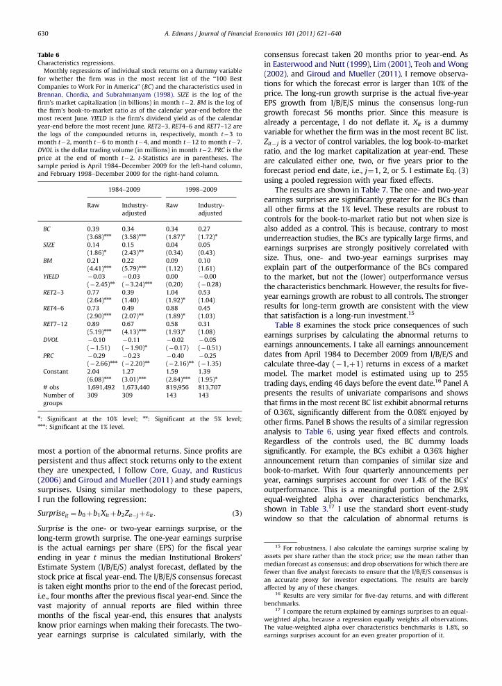
Table 6Characteristics regressions.
Monthly regressions of individual stock returns on a dummy variable
for whether the firm was in the most recent list of the ‘‘100 Best
Companies to Work For in America’’ (BC) and the characteristics used in
Brennan, Chordia, and Subrahmanyam (1998). SIZE is the log of the
firm’s market capitalization (in billions) in month t�2. BM is the log of
the firm’s book-to-market ratio as of the calendar year-end before the
most recent June. YIELD is the firm’s dividend yield as of the calendar
year-end before the most recent June. RET2–3, RET4–6 and RET7–12 are
the logs of the compounded returns in, respectively, month t�3 to
month t�2, month t�6 to month t�4, and month t�12 to month t�7.
DVOL is the dollar trading volume (in millions) in month t�2. PRC is the
price at the end of month t�2. t-Statistics are in parentheses. The
sample period is April 1984–December 2009 for the left-hand column,
and February 1998–December 2009 for the right-hand column.
1984–2009 1998–2009
Raw Industry-
adjusted
Raw Industry-
adjusted
BC 0.39 0.34 0.34 0.27
(3.68)nnn (3.58)nnn (1.87)n (1.72)n
SIZE 0.14 0.15 0.04 0.05
(1.86)n (2.43)nn (0.34) (0.43)
BM 0.21 0.22 0.09 0.10
(4.41)nnn (5.79)nnn (1.12) (1.61)
YIELD �0.03 �0.03 0.00 �0.00
(�2.45)nn (�3.24)nnn (0.20) (�0.28)
RET2–3 0.77 0.39 1.04 0.53
(2.64)nnn (1.40) (1.92)n (1.04)
RET4–6 0.73 0.49 0.88 0.45
(2.90)nnn (2.07)nn (1.89)n (1.03)
RET7–12 0.89 0.67 0.58 0.31
(5.19)nnn (4.13)nnn (1.93)n (1.08)
DVOL �0.10 �0.11 �0.02 �0.05
(�1.51) (�1.90)n (�0.17) (�0.51)
PRC �0.29 �0.23 �0.40 �0.25
(�2.66)nnn (�2.20)nn (�2.16)nn (�1.35)
Constant 2.04 1.27 1.59 1.39
(6.08)nnn (3.01)nnn (2.84)nnn (1.95)n
# obs 1,691,492 1,673,440 819,956 813,707
Number of
groups
309 309 143 143
n: Significant at the 10% level; nn: Significant at the 5% level;nnn: Significant at the 1% level.
15 For robustness, I also calculate the earnings surprise scaling by
assets per share rather than the stock price; use the mean rather than
median forecast as consensus; and drop observations for which there are
fewer than five analyst forecasts to ensure that the I/B/E/S consensus is
an accurate proxy for investor expectations. The results are barely
affected by any of these changes.16 Results are very similar for five-day returns, and with different
benchmarks.17 I compare the return explained by earnings surprises to an equal-
weighted alpha, because a regression equally weights all observations.
The value-weighted alpha over characteristics benchmarks is 1.8%, so
earnings surprises account for an even greater proportion of it.
A. Edmans / Journal of Financial Economics 101 (2011) 621–640630
most a portion of the abnormal returns. Since profits arepersistent and thus affect stock returns only to the extentthey are unexpected, I follow Core, Guay, and Rusticus(2006) and Giroud and Mueller (2011) and study earningssurprises. Using similar methodology to these papers,I run the following regression:
Surpriseit ¼ b0þb1Xitþb2Zit�jþeit : ð3Þ
Surprise is the one- or two-year earnings surprise, or thelong-term growth surprise. The one-year earnings surpriseis the actual earnings per share (EPS) for the fiscal yearending in year t minus the median Institutional Brokers’Estimate System (I/B/E/S) analyst forecast, deflated by thestock price at fiscal year-end. The I/B/E/S consensus forecastis taken eight months prior to the end of the forecast period,i.e., four months after the previous fiscal year-end. Since thevast majority of annual reports are filed within threemonths of the fiscal year-end, this ensures that analystsknow prior earnings when making their forecasts. The two-year earnings surprise is calculated similarly, with the
consensus forecast taken 20 months prior to year-end. Asin Easterwood and Nutt (1999), Lim (2001), Teoh and Wong(2002), and Giroud and Mueller (2011), I remove observa-tions for which the forecast error is larger than 10% of theprice. The long-run growth surprise is the actual five-yearEPS growth from I/B/E/S minus the consensus long-rungrowth forecast 56 months prior. Since this measure isalready a percentage, I do not deflate it. Xit is a dummyvariable for whether the firm was in the most recent BC list.Zit� j is a vector of control variables, the log book-to-marketratio, and the log market capitalization at year-end. Theseare calculated either one, two, or five years prior to theforecast period end date, i.e., j¼1, 2, or 5. I estimate Eq. (3)using a pooled regression with year fixed effects.
The results are shown in Table 7. The one- and two-yearearnings surprises are significantly greater for the BCs thanall other firms at the 1% level. These results are robust tocontrols for the book-to-market ratio but not when size isalso added as a control. This is because, contrary to mostunderreaction studies, the BCs are typically large firms, andearnings surprises are strongly positively correlated withsize. Thus, one- and two-year earnings surprises mayexplain part of the outperformance of the BCs comparedto the market, but not the (lower) outperformance versusthe characteristics benchmark. However, the results for five-year earnings growth are robust to all controls. The strongerresults for long-term growth are consistent with the viewthat satisfaction is a long-run investment.15
Table 8 examines the stock price consequences of suchearnings surprises by calculating the abnormal returns toearnings announcements. I take all earnings announcementdates from April 1984 to December 2009 from I/B/E/S andcalculate three-day (�1,þ1) returns in excess of a marketmodel. The market model is estimated using up to 255trading days, ending 46 days before the event date.16 Panel Apresents the results of univariate comparisons and showsthat firms in the most recent BC list exhibit abnormal returnsof 0.36%, significantly different from the 0.08% enjoyed byother firms. Panel B shows the results of a similar regressionanalysis to Table 6, using year fixed effects and controls.Regardless of the controls used, the BC dummy loadssignificantly. For example, the BCs exhibit a 0.36% higherannouncement return than companies of similar size andbook-to-market. With four quarterly announcements peryear, earnings surprises account for over 1.4% of the BCs’outperformance. This is a meaningful portion of the 2.9%equal-weighted alpha over characteristics benchmarks,shown in Table 3.17 I use the standard short event-studywindow so that the calculation of abnormal returns is

Table 7Earnings surprises.
Regressions of earnings surprises on a dummy variable for whether
the firm was in the most recent list of the ‘‘100 Best Companies to Work
For in America’’ (BC) and controls (BM, log book-to-market and SIZE, log
market equity) calculated at the previous year-end. The 1- (2-) year
earnings surprise is the actual EPS minus the I/B/E/S median analyst
forecast 8 (20) months prior to the end of the forecast period, scaled by
the stock price. The long-term growth surprise is the actual five-year
annualized EPS growth rate minus the I/B/E/S median analyst long-term
growth forecast from 56 months earlier. The Best Company dummy and
control variables are taken from the same month as the I/B/E/S median
forecast. Panel A (B) contains the results for 1- (2-) year earnings
surprises; Panel C contains the results for long-term growth surprises.
All coefficients are multiplied by 1,000. All regressions include year fixed
effects and a constant, not reported for brevity. t-Statistics are in
parentheses. The sample period is April 1984–December 2009.
(1) (2) (3)
Panel A: 1-Year earnings
BC 3.63 3.17 �1.14
(5.26)nnn (4.60)nnn (�1.63)
BM �1.21 �0.41
(�12.26)nnn (�4.01)nnn
SIZE 1.80
(31.26)nnn
# obs 75,813 72,164 72,164
Panel B: 2-Year earnings
BC 3.89 4.02 �0.10
(4.69)nnn (4.84)nnn (�0.12)
BM 0.41 1.23
(3.00)nnn (8.80)nnn
SIZE 1.93
(23.82)nnn
# obs 51,076 49,156 49,156
Panel C: Long-term growth
BC 2.27 3.55 1.46
(4.08)nnn (6.37)nnn (2.57)nnn
BM 2.82 3.34
(26.72)nnn (30.52)nnn
SIZE 1.02
(16.89)nnn
# obs 34,710 33,510 33,510
nnn: Significant at the 1% level.
Table 8Earnings announcement returns.
(�1,þ1) abnormal returns to quarterly earnings announcements.
Abnormal returns are calculated above a market model in which the
coefficients are estimated over a 255-day period ending 46 days before
the earnings announcement. Panel A compares the average announce-
ment returns to firms included in the most recent list of the ‘‘100 Best
Companies to Work For in America’’ with the returns to all other firms.
Panel B regresses announcement returns on a dummy variable for
whether the firm was in the most recent Best Companies list (BC) and
controls (BM, log book-to-market and SIZE, log market equity) calculated
at the previous year-end. These regressions include year fixed effects
and a constant, not reported for brevity. t-Statistics are in parentheses.
The sample period is April 1984–December 2009.
Panel A: Univariate comparisons
Best Company Other firms
CAR 0.36 0.08
# obs 5,241 311,328
t-Stat (difference from 0) (40.57)nnn (5.01)nnn
t-Stat (difference in means) (2.20)nn
Panel B: Regressions (1) (2) (3)
BC 0.29 0.43 0.36
(2.36)nn (3.49)nnn (2.83)nnn
BM 0.31 0.33
(17.17)nnn (17.37)nnn
SIZE 0.03
(3.12)nnn
# obs 316,569 296,826 296,826
nn: Significant at the 5% level; nnn: Significant at the 1% level.
A. Edmans / Journal of Financial Economics 101 (2011) 621–640 631
relatively insensitive to the benchmark asset pricing modelused. Therefore, studying earnings announcements alsoaddresses the concern that the abnormal returns stem froma yet-to-be-discovered risk factor missing from the Carhart(1997) model. Moreover, given post-earnings announce-ment drift (e.g., Bernard and Thomas, 1989), earningssurprises may account for an even greater proportion ofthe total excess returns. These results are also consistentwith La Porta, Lakonishok, Shleifer, and Vishny (1997), whofind that positive earnings surprises account for a mean-ingful proportion of the outperformance of value overglamour portfolios.
4.4. Longevity of outperformance
I now study the longevity of the excess returns. If theyresult from mispricing of employee satisfaction rather thanrisk, then one might expect the drift associated with listinclusion to decline over time, for two reasons. First, satisfac-tion is not a permanent characteristic—as shown in Table 1,
one-third of firms drop off the list each year. If a firm’ssatisfaction declines over time, it no longer enjoys top-100motivation, recruitment, and retention and so should gen-erate smaller outperformance. Put differently, the value ofthe intangible asset ignored by the market is lower, so thereis less mispricing. Second, even for firms that remain on thelist for several years, the mispricing may be corrected overtime as the market slowly learns about their value, forexample, through their releases of tangible news such asearnings. However, as shown by the prior research summar-ized in Section 2.2, this correction can take over five years.
The prior literature on long-run drift calculates long-evity of outperformance in two main ways. The first is thecumulative abnormal return (CAR). It starts by calculatinga stock’s benchmark-adjusted return in month t after the‘‘event.’’ The CAR up to month t is obtained by anarithmetic sum of the abnormal returns from month 1to month t, and the portfolio return is an equally weightedaverage of the returns on each stock affected by the event.The second is buy-and-hold returns (BHAR). This involvescalculating a stock’s benchmark-unadjusted return frommonth s to month t by geometrically compounding itsmonthly returns. The benchmark returns over that periodare calculated separately, and then subtracted from thereturn on each stock. The months s and t are typicallychosen to coincide with years (e.g., 1–12, 13–24) whicheffectively assumes rebalancing to equal-weight at thestart of each year. This is to ensure that returns are notdriven by the extreme performance of a few stocks in theportfolio. Conrad and Kaul (1993) argue that the BHARmethod is more accurate for statistical reasons.

18 Comparing newly added versus newly dropped companies leads
to economically significant differences, but not statistical significance
since there are too few added and dropped stocks to draw inferences.19 This prediction assumes that capitalization takes at least a few
weeks. If it occurs before the start of the return compounding window,
Portfolio III should earn zero abnormal returns (as should all portfolios).
A. Edmans / Journal of Financial Economics 101 (2011) 621–640632
The results of these two methods are presented inPanels A and B of Table 9. Panel A shows that the CARscontinue to grow through month 54, but are virtually zerobetween months 54 and 60. The BHAR results in Panel Bare consistent: the returns drop from 2% to 3% in year 4 toclose to zero in year 5 and become insignificant in allspecifications. Both panels suggest that, as found by priorliterature, it takes several years before the abnormalreturns start to decline. However, in contrast to Agrawal,Jaffe, and Mandelker (1992), Lakonishok, Shleifer, andVishny (1994), Spiess and Affleck-Graves (1995),Loughran and Ritter (1995), and Loughran and Vijh(1997), I find that the drift dies out in the fifth year.
The results in both panels are consistent with bothhypotheses mentioned at the start of the subsection. Thereduction in drift over time could occur either becausesome firms have dropped off the list, or because themarket has now learned of their valuable intangibles. Istart by investigating the second hypothesis—that even infirms for which satisfaction is reasonably permanent, theabnormal returns die down because the market learnsabout their intangibles over time. I conduct a similarBHAR analysis to Panel B, but focusing on firms whichremain on the list for at least the next five years—i.e.,throughout the period over which drift is calculated.Specifically, it contains firms on the 1998 list which arealso on the 1999, 2000, 2001, and 2002 lists, and so on forthe 1999–2005 lists. It also contains firms in the 1984(1993) list which are on the 1993 (1998) list. Panel Cillustrates the results; consistent with Panel B, it findsthat the returns drop markedly in the fifth year andactually become slightly negative. (Since the restrictionto firms on the list for the next five years significantlyreduces the sample size, the results in Panel C arewinsorized at the 5th and 95th percentiles to removethe effect of outliers; however, without winsorization thereturns also fall sharply and become insignificant in yearfive.) These results are consistent with a mispricing story.
I now turn to the first channel, that returns die downover time because satisfaction is not a permanent char-acteristic. I do so by studying the returns to two additionalportfolios, which contain firms that were on previous BClists but not the latest one. Portfolio II is not reformed orreweighted each year: it simply calculates the returns tothe original 74 BCs from April 1984 to December 2009,some of which drop off subsequent lists. For the Fortune
subsample, this portfolio calculates the returns of the 69BCs in the 1998 list from February 1998 to December 2009.(I conduct this particular analysis separately for the Fortune
subsample to allow comparison with Table 4 as well asTable 3.) Portfolio III includes only companies dropped fromthe list. Specifically, it is created on March 1, 1993 andincludes any companies that were in the 1984 list but notin the 1993 list. On February 1, 1998, any companies thatwere in the 1993 list but not in the 1998 list are added, andso on. If a firm is later added back to the list, it is removedfrom Portfolio III. (For the Fortune subsample, it is createdon February 1, 1999.) Like Portfolio I, Portfolio III includesfirms that go public after list formation.
Portfolio II should outperform its benchmark, since itcontains firms with high satisfaction for at least part of the
period. It should also underperform Portfolio I, since thelatter represents the most up-to-date list. On the otherhand, if Portfolio II performs similarly to Portfolio I, thiswould imply that the previous results were driven by asingle portfolio: the 1984 (or 1998) list, and thus onlyaround 70 firms, rather than the 244 firms across the fulltime period. It would also suggest that the non-perma-nence of employee satisfaction is not a reason for thereduction in drift over time. The hypothesis for the relativeperformance of Portfolios I–II is tentative as it is difficult toevaluate rigorously: since the portfolios contain manycommon stocks, their returns will be similar and likelystatistically indistinguishable. However, we can still verifywhether the differences are of the hypothesized sign.18
I also predict that Portfolio III performs worse thanPortfolios I–II, since the former contains companies out-side the Top 100 for satisfaction. Whether it also under-performs its benchmarks depends on the market’sincorporation of intangibles. If the market fully capitalizessatisfaction, the removal of a company from the listsignals that this variable has declined from previousexpectations. Therefore, if satisfaction is positively corre-lated with performance, Portfolio III should earn negativereturns.19 However, if satisfaction is important but notincorporated by the market, such a prediction is notgenerated. In the extreme, if the BC list is completelyignored, satisfaction only feeds through to returns whenits benefits manifest in future tangible outcomes. Hence,the abnormal return of firm i depends on its level ofemployee welfare compared to the average firm, ratherthan compared to the market’s previous assessment offirm i’s level of welfare. If firm i is outside the Top 100, itmay still exhibit above-average satisfaction (e.g., be in theTop 200) and thus generate superior returns.
Panel D of Table 9 illustrates the results. The returns toPortfolio II are positive over all time-periods, benchmarks,and weighting methodologies, and often significant, but itunderperforms Portfolio I in all 12 specifications. Theseresults suggest that employee satisfaction is not a perma-nent characteristic and list updates contain useful infor-mation, potentially explaining why outperformance isparticularly strong over 1998–2009. In the Fortune sub-period, the list was updated every year, whereas for1984–1997, it was updated only once in a 14-year period.Indeed, the weaker results for the 1984 Portfolio II arisebecause it contained firms such as Polaroid, Delta Airlines,Dana, and Armstrong that featured only in the 1984 listand suffered very weak performance from 1993 onwards.Also as predicted, Portfolio III underperforms Portfolio I inall 12 specifications, and Portfolio II in all specificationsexcept for the equal-weighted specification from 1984 to2009. This strong performance disappears when value-weighting (or, in unreported results, winsorizing). How-ever, Portfolio III only underperforms its benchmarks for

Table 9Longevity analysis.
Panel A calculates cumulative abnormal returns (CAR) to portfolios of the ‘‘100 Best Companies to Work For in America’’ in calendar time. The abnormal
return of stock in event month t is calculated by subtracting its benchmark return t months after list inclusion. The CAR through month t is an arithmetic sum
of the abnormal returns from months 1 through t. Panel B calculates the buy-and-hold returns (BHAR). It first geometrically compounds the unadjusted returns
of a Best Company from month 1–12, 13–24, etc. and then subtracts the geometrically compounded benchmark return over the same period. Panel C calculates
the BHAR to companies that remain on the list for the following five years, winsorizing at the 5th and 95th percentiles. Panel D contains monthly regressions of
the returns of Portfolios II and III on the four Carhart (1997) factors, MKT, HML, SMB, and MOM. Portfolio II is the original 1984 (1998) Best Companies list and is
not updated with subsequent lists. Portfolio III contains only companies dropped from a prior list. The alpha is the excess risk-adjusted return. t-Statistics are in
parentheses. The sample period is April 1984–December 2009 for Panels A–C and given in the headings for Panel D.
Panel A: CARs CAR over
Month Market Industry Characteristics
6 2.11 2.21 1.5612 5.57 4.72 4.7618 7.26 6.65 5.8024 10.36 8.66 8.8230 11.50 10.36 9.3236 15.73 12.88 12.5442 18.63 15.92 14.0948 21.03 17.33 16.0354 24.10 20.57 18.6860 24.21 20.68 18.66
Panel B: BHARs BHAR over
Months Market Industry Characteristics
1–12 5.07 4.53 4.84
(2.11)nn (1.94)n (1.90)n
13–24 2.66 2.24 2.66
(1.88)n (1.73)n (1.91)n
25–36 3.32 2.63 1.87
(2.41)nn (2.05)n (1.36)
37–48 3.35 2.90 1.94
(2.44)nn (2.25)nn (1.61)
49–60 0.33 0.81 0.27
(0.24) (0.62) (0.21)
Panel C: BHARs of firms on list for 5 years
BHAR over
Months Market Industry Characteristics
1–12 9.47 6.97 6.81
(5.28)nnn (4.34)nnn (3.63)nnn
13–24 6.63 4.30 5.41
(3.81)nnn (2.82)nnn (3.18)nnn
25–36 3.10 2.13 2.45
(1.90)n (1.49) (1.50)
37–48 2.95 2.28 2.38
(1.95)n (1.62) (1.68)n
49–60 �0.36 �0.07 �0.82
(�0.23) (�0.04) (�0.56)
Panel D: Alphas 1984–2009: excess returns over 1998–2009: excess returns over
Risk-free Industry Characteristics Risk-free Industry Characteristics
Equal-weighted
a, II 0.23 0.12 0.13 0.44 0.28 0.34
(2.15)nn (1.44) (1.41) (2.97)nnn (2.55)nn (2.50)nn
a, III 0.30 0.20 0.21 0.34 0.26 0.27
(2.68)nnn (2.16)nn (2.36)nn (1.75)n (1.82)n (1.96)n
Value-weighted
a, II 0.23 0.16 0.15 0.24 0.08 0.11
(2.31)nn (1.85)n (2.36)nn (1.17) (0.62) (0.87)
a, III 0.16 0.04 0.04 �0.21 �0.29 �0.19
(1.44) (0.34) (0.63) (�1.08) (�2.13)nn (�1.44)
# obs 309 for II, 202 for III 143 for II, 131 for III
n: Significant at the 10% level; nn: Significant at the 5% level; nnn: Significant at the 1% level.
A. Edmans / Journal of Financial Economics 101 (2011) 621–640 633

20 http://www.socialinvest.org/resources/mfpc/screening.cfm.21 The other screens are alcohol, tobacco, gambling, defense/weapons,
animal testing, products/services, environment, human rights, and com-
munity investment. For the first four screens, there is a fourth option of
‘‘No Investment,’’ which is stronger than Restricted Investment and
denotes that the fund will not invest in any company that produces these
products. There is no such option for the labor or employment screens.22 http://www.socialfunds.com/funds/chart.
cgi?sfChartId=SocialþIssues.23 The other screens are shareholder advocacy, community invest-
ment, environment, human rights, employment, product safety, weap-
ons, animal rights, nuclear power, and alcohol/tobacco/gambling.
A. Edmans / Journal of Financial Economics 101 (2011) 621–640634
the Fortune subsample when value-weighting (and onlysignificantly compared to the industry benchmark), andoutperforms significantly in some specifications. Thisresult further suggests that the market did not fully reactwhen the companies in Portfolio III were initially added tothe list.
Overall, the results in all four panels of Table 9 suggestthat the abnormal returns of BCs abate over time, bothbecause employee satisfaction is not a permanent char-acteristic, and the market slowly learns about this intan-gible. The duration of outperformance, of approximatelyfour years, is slightly lower than some prior studies andthus implies a lower level of mispricing.
5. Discussion
Section 4 has shown a significant correlation betweenemployee satisfaction and future stock returns that isrobust to controls for risk, industries, firm characteristics,and outliers. There are a number of potential explanationsfor this association:
Hypothesis A: Employee satisfaction causes superiorfuture stock returns, and this link was not fully valued bythe market.
Hypothesis B: Employee satisfaction is irrelevant forshareholder value, but list inclusion causes higher returnsvia irrational market reactions or demand from SRI funds.
Hypothesis C: Employee satisfaction is irrelevant forshareholder value, but list inclusion causes higher returnsbecause the market erroneously believes it is detrimentalto value. Listed firms thus trade at an initial discount, andthe higher returns are a correction of this.
Hypothesis D: Expectations of superior future stockreturns cause high satisfaction today.
Hypothesis E: There is no causal relationship in eitherdirection between satisfaction and stock returns, but athird variable causes both.
The results of Tables 7 and 8 provide support forHypothesis A: that employee satisfaction is not directlycapitalized, but only affects the stock price when it subse-quently manifests in tangible outcomes that are valued bythe market. The evidence of Table 9, that the abnormalreturns eventually die out with a longevity similar to othermispricing studies, is also consistent with this hypothesis.This section evaluates the alternative explanations.
As stated in the Introduction, stock returns haveseveral advantages as a dependent variable: they arecritical for the paper’s three goals. However, they alsohave some limitations. While they should incorporate allchannels through which satisfaction can affect funda-mental value, they may also be influenced by factorsunrelated to fundamental value, such as irrational spec-ulation. Thus, even if there is causality, it could be listinclusion per se rather than satisfaction that is causingsuperior returns. Hypothesis B is that the superior returnsdid not stem from a true increase in firm value. Forexample, satisfaction may be irrelevant for shareholdervalue, but the market erroneously believes that a relation-ship exists and reacts irrationally positively to list inclu-sion. This hypothesis is contradicted by the superiorearnings surprises of the BCs, which represent an increase
in fundamental value. Moreover, Gilbert, Lochstoer,Kogan, and Ozyildirim (2010) and Huberman and Regev(2001) show that irrational reactions to non-informationare concentrated immediately after the announcement ofirrelevant news. Here, the event-study window is excludedfrom the return calculation.
A similar explanation is that list inclusion led to buyingby SRI funds because it allows the stocks to pass SRI screens;if demand curves are downward-sloping, this raises prices.Such purchases may take time to be executed and need notoccur within the month of list announcement. In addition tothe earnings announcement results, an additional piece ofevidence against this explanation is the mild outperfor-mance of the dropped companies in Portfolio III. For a moresystematic evaluation of this hypothesis, I study whetherSRI funds indeed are overweighting the BCs, and whetherthey increased this weighting over time. There is substantialheterogeneity across SRI funds and many screen on factorsorthogonal to employee satisfaction, such as animal testingand environmental protection. I therefore must be careful toselect funds that use employment screens in particular. Mymain data source is the Social Investment Forum,20 whichcontains details of each SRI fund and 11 different screeningcriteria, two of which are labor relations and employment/equality. For each fund and criterion, there are threecategories. Positive Investment denotes that the fund ismore likely to invest in a firm that surpasses an upper barfor the criterion, Restricted Investment denotes that thefund will seek to avoid firms that fall below a lower bar, andNo Screen denotes that the fund does not use that criter-ion.21 The classifications for labor relations and employ-ment/equality are highly correlated, with only one fundhaving a different designation between the two. I supple-ment this source with data from SocialFunds,22 whichprovides a similar table. One of its ten screens is employ-ment.23 There is considerable overlap between the two datasources; when there is disagreement, I read the fundprospectus to see whether it mentions an employmentscreen. If it does not, I call the fund to verify whether ituses such a screen. For example, such calls uncovered thatthe Ariel Fund does not use employment screens, contraryto the data from SocialFunds. I also called all major fundfamilies (even when there was no disagreement betweenthe data sources) to verify that the screening criteria havenot changed over time, and that the family did not pre-viously have a fund that screened on employment that isnow defunct and thus not in either data source. I drop fundsthat invest exclusively overseas or in bonds, or are not in theCDA/Spectrum database, from which I obtain fund holdings.

Table 10List of employment funds.
SRI funds that invest in domestic equity and use labor or employment screens. The main data sources are the Social Investment Forum and SocialFunds.
Any conflicts were resolved by reading the fund prospectus or calling the fund. (P) denotes that the fund employs a Positive Investment screen on labor or
employment, and (R) denotes a Restricted Investment screen.
AHA Socially Responsible Equity (P) LKCM Acquinas Small Cap (R)
Appleseed (P) LKCM Acquinas Value (R)
Calvert Aggressive Allocation (P) MMA Praxis Core Stock (P)
Calvert Capital Accumulation (P) MMA Praxis Growth Index (P)
Calvert Conservative Allocation (P) MMA Praxis Intermediate Income (P)
Calvert Global Alternative Energy (P) MMA Praxis International (P)
Calvert International Opportunities (P) MMA Praxis Small Cap (P)
Calvert Large Cap Growth (P) MMA Praxis Value Index (P)
Calvert Mid Cap Value (P) Neuberger Berman Socially Responsible (P)
Calvert Moderate Allocation (P) New Alternatives (P)
Calvert New Vision Small Cap (P) Parnassus (P)
Calvert Small Cap Value (P) Parnassus Mid-Cap (P)
Calvert Social Index (P) Parnassus Small-Cap (P)
Calvert Social Investment Balanced (P) Parnassus Workplace (P)
Calvert Social Investment Enhanced Equity (P) Pax World Balanced (P)
Calvert Social Investment Equity (P) Pax World Growth (P)
Calvert World Values International (P) Pax World High Yield (P)
Domini Social Equity (P) Pax World Value (P)
Dreyfus Premier Third Century (R) Pax World Women’s Equity (R)
Epiphany Faith and Family Values 100 (P) Sentinel Sustainable Core Opportunities (P)
Flex-Funds Total Return Utilities (R) Sentinel Sustainable Emerging Companies (P)
Green Century Equity (P) TIAA CREF Inst Social Choice Equity (P)
Integrity Growth and Income (R) Vanguard FTSE Social Index Fund (R)
Legg Mason Partners Social Awareness (P) Walden Social Balanced (P)
LKCM Acquinas Growth (R) Walden Social Equity (P)
A. Edmans / Journal of Financial Economics 101 (2011) 621–640 635
Table 10 contains the final list of ‘‘employment funds’’which use either a Positive or Restricted Investment screenon labor or employment.24
I run the following regression:
EOit ¼ c0þc1Xitþc2Zitþeit : ð4Þ
EOit is the percentage ownership of stock i across allemployment funds in Table 10 at the end of Decemberof year t. Xit is a dummy variable for whether the firm wasin the most recent BC list, and Zit is a vector of controlvariables. Following Hong and Kacperczyk (2009), I usethe following controls: log size, log M/B, the inverse stockprice, S&P 500 dummy, and Nasdaq dummy (all measuredat the end of year t), as well as the standard deviation ofdaily returns and average monthly return (measured inyear t). I also use industry dummy variables.25 Also as inHong and Kacperczyk (2009), I run a panel regressionwith year fixed effects and cluster standard errors at theindustry level, since a fund’s investment in a particularstock may increase (reduce) its probability of owning anindustry peer for specialization (diversification) reasons.
24 List inclusion can affect the holdings of funds with both Positive
and Restricted screens, since it may directly cause a positively screening
fund to buy the stock, and remove limitations previously preventing a
restrictively screening fund from buying the stock. Therefore, the main
specification includes employment funds that impose both types of
screens, but I also run the results focusing only on funds that positively
screen.25 HK do not use industry dummy variables because their definition
of sin stocks is at the industry level; they instead use the industry beta.
Industry dummies are feasible in the present setting, and control for
broader differences across industries than their betas.
The results are very similar using Fama-MacBeth (1973)and are available upon request.
Table 11 shows that employment funds indeed over-weight the BCs. To investigate whether overweighting hasincreased over time, I add an additional regressor, Yit, toEq. (4), where Yit¼(Year�1984)�Xit; it is significant. I nextcalibrate the extent to which this increase in demand canexplain the superior returns. Employment funds owned$5m of BC stock in 1984 and $1,653m in 2007. (To form anupper bound on the excess return that can be explained byincreased demand, I take the 2007 figures as they are thehighest.) The total value of the BCs was $303,169m in 1984and $1,703,218m in 2007. Thus, the increase in employ-ment funds’ ownership of BC stock is driven in part by theincrease in market value of the BCs rather than newpurchases. Again to form an upper bound, I assume thatthe entire $1,648m increase stems from new purchases.The next step is to turn this into a percentage change indemand. To maximize the percentage change, I take the1984 value of BCs as the denominator, which translates intoa 0.54% increase. The effect on stock prices is given by
DP¼ 0:0054=e, ð5Þ
where e is the absolute price elasticity of demand. Estimatesof e range widely: Shleifer (1986) and Gompers and Metrick(2001) suggest a unit elasticity,Wurgler and Zhuravskaya(2002) estimate e¼ 8, and Scholes (1972) calibratese¼ 3,000. Using e¼ 1, again to create an upper bound,yields a 0.54% abnormal return, or only 0.02% per year.26
26 Inflows into Best Companies require outflows from other firms,
and thus reduce the performance of benchmarks. Since the outflows will

Table 11Holdings by employment funds.
Regressions of a stock’s aggregate ownership by employment funds at
year-end on a dummy variable for whether the firm was in the most
recent list of the ‘‘100 Best Companies to Work For in America’’ (BC) and
various control variables. SIZE is log market equity, MB is the log market-
to-book ratio, PRINV is the inverse of the stock price, NASDAQ and SP500
are dummy variables for inclusion in the Nasdaq and S&P 500 indexes
(all measured at year-end), STD is the standard deviation of daily stock
returns, and MORET is the average monthly return (all measured over
the year). In specifications (3) and (4), I include YEARBC, defined as
(Year�1984) �BC. The coefficients are estimated using a panel regres-
sion with industry and year dummies. Robust standard errors are
clustered at the industry level. t-Statistics are in parentheses. The
sample period is 1984–2009. Columns 1 and 3 consider funds that use
positive or restrictive employment screens. Columns 2 and 4 only
consider funds that employ positive employment screens alone. All
coefficients are multiplied by 1,000.
(1) (2) (3) (4)
All funds Positive funds All funds Positive funds
BC 0.330 0.328 �0.101 �0.083
(3.27)nnn (3.28)nnn (�0.62) (�0.52)
YEARBC 0.039 0.038
(3.49)nnn (3.35)nnn
SIZE 0.054 0.052 0.053 0.051
(8.01)nnn (7.75)nnn (7.98)nnn (7.72)nnn
MB �0.029 �0.030 �0.030 �0.030
(�2.84)nnn (�2.84)nnn (�2.89)nnn (�2.89)nnn
PRINV 0.013 0.012 0.012 0.012
(6.58)nnn (6.29)nnn (6.44)nnn (6.15)nnn
STD �0.004 �0.004 �0.004 �0.004
(�1.81)n (�1.88)n (�1.82)n (�1.89)n
MORET �0.002 �0.002 �0.002 �0.002
(�2.96)nnn (�2.92)nnn (�2.90)nnn (�2.85)nnn
NASDAQ 0.029 0.030 0.029 0.029
(1.32) (1.36) (1.31) (1.34)
SP500 0.001 �0.005 0.005 �0.001
(0.03) (�0.17) (0.17) (�0.03)
Constant �0.282 �0.273 �0.284 �0.275
(�5.91)nnn (�5.76)nnn (�5.97)nnn (�5.81)nnn
# obs 143,487 143,487 143,487 143,487
n: Significant at the 10% level; nnn: Significant at the 1% level.
A. Edmans / Journal of Financial Economics 101 (2011) 621–640636
This is substantially smaller than the 3.5% annual alpha, andso in-sample purchases cannot explain the excess returns.27
Hypothesis C is that satisfaction has no effect onshareholder value, but the market believes that it has anegative effect [owing to traditional views that it repre-sents wasteful expenditure, e.g., Taylor (1911)] and soreduced its initial valuation of the BCs. Under this hypoth-esis, the subsequent superior returns are merely
(footnote continued)
be spread over the thousands of stocks that are not Best Companies, the
outflows from a particular stock will be negligible.27 The main reason why increased ownership by employment funds
is unable to explain a significant portion of the Best Companies’
outperformance is there are very few such funds, and so they have little
price impact. I therefore rerun Eq. (4) using total institutional ownership
as the dependent variable, since institutions in aggregate hold substan-
tially more assets than employment funds. However, I find institutions
are underweighted on the Best Companies. These results remain similar
when studying only ownership by banks, insurance companies, and
other institutions, who are more likely to be constrained by social norms
(Hong and Kacperczyk, 2009). The results are available upon request.
correction of temporary undervaluation rather than anydirect benefit of satisfaction. This interpretation echoesHong and Kacperczyk (2009), who find that ‘‘sin’’ stocks’abnormal returns stemmed from their initial undervalua-tion. Again, it is list inclusion rather than satisfaction thatis causing the superior returns.
This hypothesis is contradicted by the slightly positiveevent-study returns to list inclusion shown by Faleye andTrahan (2006), which I also confirm in unreported results.An additional test is to examine whether the BCs traded ata value discount to their peers at the start of the returncompounding period. Hypotheses A and C have differentpredictions as to whether an initial discount should exist.Hypothesis A posits that the BCs are undervalued relativeto their true fundamental value (comprised of tangibleand intangible assets) since their intangible value ispartially ignored. However, it does not predict that theBCs should have lower observed valuation ratios thanpeers, because the denominator of traditional valuationratios (e.g., market-to-book) does not consider intangi-bles. For example, assume that firm 1 has $2bn of tangibleassets and thus a true value of $2bn; firm 2 has $2bn oftangible assets and has spent $1bn on intangibles. UnderHypothesis A, firm 2’s intangibles are valuable and so itstrue value is $3bn, but it trades at $2.4bn as the marketonly partially incorporates intangibles. Thus, firm 1 (2)exhibits an M/B ratio of 1 (1.2) and so firm 2’s subsequentabnormal returns arise not because it trades at an initialdiscount, but because it has valuable intangibles whichwere not fully priced initially. Under Hypothesis C, firm2’s intangibles are worthless and so its true value is also$2bn, but the market values it at $1.5bn because it infersthat wasteful expenditure on intangibles implies moregeneral agency problems. Firm 2 therefore trades at aninitial M/B of 0.75 and thus at a discount to firm 1; itssubsequent abnormal returns result entirely from acorrection of this discount.
I therefore run the following regression:
VALit ¼ d0þd1Xitþd2Zit�1þeit , ð6Þ
at the beginning of each return compounding window.VALit is the valuation of stock i at the start of the returncompounding period in year t (i.e., end of March fort¼1984, February for t¼1993, January for 1998–2009).Similar to Hong and Kacperczyk (2009), I use threevaluation ratios: the log market-to-book ratio (M/B), thelog price-to-earnings ratio (P/E), and the log of the ratio ofaggregate value to earnings before interest, tax, deprecia-tion, and amortization (AV/EBITDA).28 I drop observationsfor which the denominator is negative. Xit is a dummyvariable for whether the firm is in that month’s BC list,and Zit�1 is a vector of control variables measured as ofDecember of the previous year. Following Hong andKacperczyk, I use the firm’s return on equity (ROE) aswell as the next three year’s ROEs, R&D as a fraction ofsales, a dummy variable if R&D is missing, and an S&P 500
28 Hong and Kacperczyk (2009) use the price-to-EBITDA ratio. Since
the EBITDA represents profits to both debtholders and equityholders,
I use the aggregate value of both debt and equity in the numerator.
AV/EBITDA is unaffected by changes in capital structure.

Table 12Valuation regressions.
Regressions of a stock’s valuation on a dummy variable for whether the
firm is in the current list of the ‘‘100 Best Companies to Work For in
America’’ (BC) and various control variables. The three valuation measures
are MB, the log market-to-book ratio, PE, the log price-to-earnings ratio,
and AVEBITDA, the log ratio of aggregate value to EBITDA, and measured at
the end of each month in which a Best Companies list was published, i.e.,
March 1984, February 1993, and January 1998–2007. I drop observations
for which the denominator of the valuation ratio is negative. The control
variables are all measured at December of the previous year: ROE is the
return on equity, FROE, F2ROE, and F3ROE are the returns on equity for the
next three years, RDSALES is the ratio of R&D to sales, RDMISS is a dummy
variable for whether R&D is missing, and SP500 is a dummy variable for
inclusion in the S&P 500 index. The coefficients are estimated using Fama-
MacBeth (1973). t-Statistics are in parentheses.
(1) (2) (3)
MB PE AVEBITDA
BC 0.384 0.092 0.145
(9.24)nnn (2.14)n (3.57)nnn
ROE 0.006 �0.297 �0.063
(0.49) (�1.17) (�1.07)
RDSALES 0.030 2.086 0.803
(1.09) (4.73)nnn (1.81)n
RDMISS �0.100 �0.017 �0.055
(�4.46)nnn (�0.89) (�2.06)n
SP500 0.583 0.330 0.168
(6.62)nnn (4.65)nnn (3.64)nnn
FROE 0.038 0.038 0.006
(1.25) (0.88) (0.79)
F2ROE 0.008 0.070 0.016
(1.68) (1.04) (0.93)
F3ROE 0.003 0.008 0.000
(2.48)nn (2.23)nn (0.22)
Constant �0.083 2.105 2.013
(�0.33) (11.06)nnn (10.74)nnn
# obs 47,097 35,258 39,381
Number of groups 12 12 12
n: Significant at the 10% level; nn: Significant at the 5% level; nnn:
Significant at the 1% level.
29 Furthermore, the Best Companies survey does not simply ask
employees the general question of rating their satisfaction, which could
indeed lead to optimistic employees reporting high satisfaction. Instead,
the survey covers very specific questions, such as communication to
employees, corporate philanthropy, and diversity, which aim to speci-
fically target satisfaction rather than optimism.30 An alternative approach would be to use random variation in
some firm-specific characteristic that was causal for employee satisfac-
tion but has no direct effect on stock returns. Unfortunately, I have been
unable to identify such an appropriate instrument. For example, ‘‘natural
experiments’’ such as exploiting labor law regulatory change are not
firm-specific.
A. Edmans / Journal of Financial Economics 101 (2011) 621–640 637
dummy. I estimate Eq. (6) using Fama-MacBeth (1973),adjusting standard errors for potential autocorrelation.
The results are shown in Table 12. The BCs exhibit higher
valuation ratios based on all three measures. These findingsare inconsistent with Hypothesis C but consistent withHypothesis A, as well as Gompers, Ishii, and Metrick (2003)who show that firms with strong governance earned abnor-mal returns while trading at a valuation premium at the startof the return window. The higher ratios suggest that themarket is at least partially valuing the intangibles. This resultis also consistent with the drift studies summarized inSection 2.2, which find that the market generally valuescorporate events in the correct direction, but significantlyunderestimates the magnitudes. Indeed, in the abovenumerical example, firm 2 trades at an initial premium.
Since the setting is not a natural experiment withrandom assignment of employee satisfaction to firms,non-causal explanations also exist. Hypothesis D is thatsuperior performance leads to satisfaction. The use of stockreturns as a dependent variable addresses concerns ofreverse causation in the absence of private information—
past, current, and expected future profitability should all beincorporated in the current stock price, and so profitablefirms should not outperform going forward. However, if
employees have superior information about their firm’sfuture stock returns, those with positive information mayreport higher satisfaction today. This explanation is unlikelyfor a number of reasons. Existing empirical studies suggestthat employees do not have private information: Benartzi(2001) shows that employees make incorrect decisionswhen allocating their 401(k) accounts to company stock,and Bergman and Jenter (2007) find that firms are able tolower total compensation by granting their workers over-valued options in lieu of salary. Even if employees do havesuperior information, it is likely to be about near-termreturns, given that managers are unable to forecast returnspast 100 days (Jenter, Lewellen, and Warner, 2011). Sincethey must return the questionnaires by the end of June,seven months before the start of the return compoundingwindow the following February 1, this will not affect theresults. It is also plausible that employees who predicthigher future returns will perceive the stock as undervaluedtoday, potentially reducing satisfaction.29
Hypothesis E is that the link between satisfaction andreturns arises because a third unobservable variable causesboth, such as good management (Bloom, Kretschmer, andVan Reenen, 2009; Bloom et al., 2011)—i.e., the BC dummyproxies for an omitted variable. While I rule out correlationwith industries, factor loadings, and an extensive list ofobservable characteristics, by their very nature, unobserva-bles cannot be used as regressors. The standard solution is tointroduce firm fixed effects to absorb the unobservables andidentify purely on within-firm changes in the variable inquestion. This approach cannot be used here because fixedeffects require the unobservables to be constant over time,but a change in satisfaction could be caused by changes inmanagement practices. In addition, there is limited within-firm variation in list inclusion: many firms remain in the listfor several years, and a firm removed from the list may stillexhibit significantly above-average satisfaction (e.g., be inthe Top 200). Thus, such an approach would be biasedtowards finding no relationship (Zhou, 2001).30
If the results were entirely driven by a combination ofHypotheses D and E, then satisfaction has no causal effecton returns and the introduction of employee-friendlyprograms would have no impact. However, other conclu-sions from this paper would be unaffected. It still remainsthat the market does not incorporate intangibles (be theysatisfaction, good management, or workers’ private infor-mation) even when made public; that investors under-react to even widely disseminated news concerning largecompanies; and that an SRI investor could have earnedexcess returns by trading on the BC list.
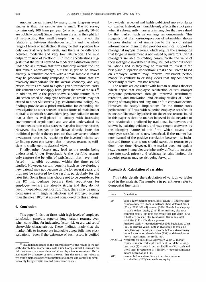
A. Edmans / Journal of Financial Economics 101 (2011) 621–640638
Another caveat shared by many other long-run eventstudies is that the sample size is small. The BC surveycontains only 100 firms per year (of which typically 50–70are publicly traded). Since these firms are all in the right tailof satisfaction, this small sample may not reflect therelationship between shareholder returns and the wholerange of levels of satisfaction. It may be that a positive linkonly exists at very high levels, and there is no differencebetween moderate and very low satisfaction. The mildoutperformance of Portfolio III in most specifications sug-gests that the results extend to moderate satisfaction levels,under the assumption that firms that drop outside the Top100 remain above-average, but this is yet to be showndirectly. A standard concern with a small sample is that itmay be predominantly composed of small firms that arerelatively unimportant for the overall economy, and anyexcess returns are hard to exploit given transactions costs.This concern does not apply here, given the size of the BCs.31
In addition, while the paper shows superior returns to anSRI screen based on employee relations, its results may notextend to other SRI screens (e.g., environmental policy). Myfindings provide an a priori motivation for extending theinvestigation to other screens: if other forms of ‘‘stakeholdercapital’’ also benefit shareholders (e.g., low pollution meansthat a firm is well-placed to comply with increasingenvironmental regulations) and are also undervalued bythe market, certain other screens may also improve returns.However, this has yet to be shown directly. Note thattraditional portfolio theory predicts that any screen reducesinvestment returns by restricting the investor’s choice set,so finding even one screen that improves returns is suffi-cient to challenge this classical view.
Finally, other factors may lead to the results beingunderstated. Under Hypothesis A, the portfolio returnsonly capture the benefits of satisfaction that have mani-fested in tangible outcomes within the time periodstudied. However, certain benefits (such as developing anew patent) may not become visible for several years, andthus not be captured by the results, particularly for thelater lists. Some firms may choose not to be considered forthe BC list, perhaps because their reputations foremployee welfare are already strong and they do notneed independent certification. Thus, there may be manycompanies with high satisfaction and stronger returnsthan the mean BC, that are not considered by this analysis.
6. Conclusion
This paper finds that firms with high levels of employeesatisfaction generate superior long-horizon returns, evenwhen controlling for industries, factor risk, or a broad set ofobservable characteristics. These findings imply that themarket fails to incorporate intangible assets fully into stockvaluations—even if the existence of such assets is verified
31 In addition to issues on the generalizability of the results to the rest
of the distribution, another issue with a small sample is that it increases the
risk that results are anomalous and driven by a few observations. This is
addressed by a battery of tests showing that the results are robust to
weighting methodologies, winsorization of outliers, and controlling simul-
taneously for systematic risk and firm characteristics.
by a widely respected and highly publicized survey on largecompanies. Instead, an intangible only affects the stock pricewhen it subsequently manifests in tangibles that are valuedby the market, such as earnings announcements. Thissuggests that the non-incorporation of intangibles, shownby prior studies, is not simply due to the lack of salientinformation on them. It also provides empirical support formanagerial myopia theories, which require the assumptionthat long-run investment is not valued by investors. Even ifmanagers are able to credibly communicate the value oftheir intangible investment, it may still not affect outsiders’valuations, and so they may be reluctant to invest in thefirst place. A separate implication is that an SRI screen basedon employee welfare may improve investment perfor-mance, in contrast to existing views that any SRI screennecessarily reduces investor returns.
The results are consistent with human relations theorieswhich argue that employee satisfaction causes strongercorporate performance through improved recruitment,retention, and motivation, and existing studies of under-pricing of intangibles and long-run drift to corporate events.However, the study’s implications for the future stockperformance of firms with superior employee satisfactionis unclear. The main hypothesis for the excess returns foundin this paper is that the market believed in the negative orzero relationship predicted by traditional frameworks andshown by existing evidence, and was caught unawares bythe changing nature of the firm, which means thatemployee satisfaction is now beneficial. If the market hasnow learned of the positive correlation between list inclu-sion and future returns, one should expect the returns to godown over time. However, if the market does not update(e.g., because intangibles are inherently difficult to incorpo-rate into stock prices) and arbitrage remains limited, thesuperior returns may persist going forward.
Appendix A. Calculation of variables
This table details the calculation of various variablesused in the analysis. The numbers in parentheses refer toCompustat line items.
Item
CalculationBM
Book equity/market equity. Book equity ¼ shareholders’equity—preferred stock þ balance sheet deferred taxes
(35) þ FASB 106 adjustment (330). Shareholders’ equity
¼ stockholders’ equity (216) if not missing, else total
common equity (60) plus preferred stock par value (130)
if both are present, else total assets (6) minus total
liabilities (181), if both are present.
Preferred stock ¼ redemption value (56), liquidating value
(10), or carrying value (130), in that order, as available.
PE
Price/Earnings. Earnings ¼ income before extraordinaryitems for common shareholders (237) þ deferred taxes
(50) þ investment tax credit (50).
AVEBITDA
Aggregate value/EBITDA. Aggregate value ¼ marketequity þ market value plus net debt. Net debt ¼ long-
term debt (9) þ debt in current liabilities (34)—cash and
short-term investments (1). EBITDA ¼ operating income
before depreciation (13).
ROE
Income before extraordinary items for commonshareholders (237)/average book equity.

A. Edmans / Journal of Financial Economics 101 (2011) 621–640 639
References
Aboody, D., Lev, B., 1998. The value relevance of intangibles: the case ofsoftware capitalization. Journal of Accounting Research 36, 161–191.
Abowd, J., 1989. The effect of wage bargains on the stock market value ofthe firm. American Economic Review 79, 774–800.
Agrawal, A., Jaffe, J., Mandelker, G., 1992. The post-merger performanceof acquiring firms: a re-examination of an anomaly. Journal ofFinance 47, 1605–1621.
Akerlof, G., Yellen, J., 1986. Efficiency Wage Models of the Labor Market.Cambridge University Press, Cambridge, UK.
Akerlof, G., 1982. Labor contracts as partial gift exchange. QuarterlyJournal of Economics 97, 543–569.
Bauer, R., Koedijk, K., Otten, R., 2005. International evidence on ethicalmutual fund performance and investment style. Journal of Bankingand Finance 29, 1751–1767.
Benartzi, S., 2001. Excessive extrapolation and the allocation of 401(k)accounts to company stock. Journal of Finance 56, 1747–1764.
Bergman, N., Jenter, D., 2007. Employee sentiment and stock optioncompensation. Journal of Financial Economics 84, 667–712.
Berk, J., Stanton, R., Zechner, J., 2010. Human capital, bankruptcy, andcapital structure. Journal of Finance 65, 891–926.
Bernard, V., Thomas, J., 1989. Post-earnings-announcement drift: delayedprice response or risk premium? Journal of Accounting Research 27,1–36.
Bloom, N., Kretschmer, T., Van Reenen, J., 2009. Work-life balance,management practices and productivity. In: Freeman, R., Shaw, K.(Eds.), International Differences in the Business Practices andProductivity of Firms. University of Chicago Press, Chicago, pp.15–54.
Bloom, N., Kretschmer, T., Van Reenen, J., 2011. Are family-friendlyworkplace practices a valuable firm resource? Strategic Manage-ment Journal 32, 343–367.
Brammer, S., Brooks, C., Pavelin, S., 2006. Corporate social performanceand stock returns: UK evidence from disaggregate measures. Finan-cial Management 35, 97–116.
Brennan, M., Chordia, T., Subrahmanyam, A., 1998. Alternative factorspecifications, security characteristics, and the cross-section ofexpected stock returns. Journal of Financial Economics 49, 345–373.
Carhart, M., 1997. On persistence in mutual fund performance. Journal ofFinance 52, 57–82.
Carlin, B., Gervais, S., 2009. Work ethic, employment contracts, and firmvalue. Journal of Finance 64, 785–821.
Chan, L., Lakonishok, J., Sougiannis, T., 2001. The stock market valuationof research and development expenditures. Journal of Finance 56,2431–2456.
Conrad, J., Kaul, G., 1993. Long-term market overreaction or biases incomputed returns? Journal of Finance 48, 39–63.
Core, J., Guay, R., Rusticus, T., 2006. Does weak governance cause weakstock returns? An examination of firm operating performance andinvestors’ expectations. Journal of Finance 61, 655–687.
Cronqvist, H., Heyman, F., Nilsson, M., Svaleryd, H., Vlachos, J., 2008. Doentrenched managers pay their workers more? Journal of Finance64, 309–339.
Daniel, K., Grinblatt, M., Titman, S., Wermers, R., 1997. Measuringmutual fund performance with characteristic-based benchmarks.Journal of Finance 52, 1035–1058.
Daniel, K., Titman, S., 1997. Evidence on the characteristics of cross-sectional variation in common stock returns. Journal of Finance 52,1–33.
Deng, Z., Lev, B., Narin, F., 1999. Science and technology as predictors ofstock performance. Financial Analysts Journal 55, 20–32.
Derwall, J., Guenster, N., Bauer, R., Koedijk, K., 2005. The eco-efficiencypremium puzzle. Financial Analysts Journal 61, 51–63.
Dhrymes, P., 1998. Socially responsible investment: Is it profitable? In:Bruce, B. (Ed.), The Investment Research Guide to Socially Respon-sible Investing. The Colloquium on Socially Responsible Investing,Plano, TX, pp. 264–284.
Diltz, J., 1995. Does social screening affect portfolio performance?Journal of Investing 4, 64–69.
Easterwood, J., Nutt, S., 1999. Inefficiency in analysts’ earnings forecasts:Systematic misreaction or systematic optimism? Journal of Finance54, 1777–1797.
Edmans, A., 2009. Blockholder trading, market efficiency, and manage-rial myopia. Journal of Finance 64, 2481–2513.
Faleye, O., Trahan, E., 2006. Is what’s best for employees best forshareholders? Unpublished working paper, Northeastern University.
Fama, E., French, K., 1997. Industry costs of equity. Journal of FinancialEconomics 43, 153–193.
Fama, E., French, K., 2008. Dissecting anomalies. Journal of Finance 63,1653–1678.
Fama, E., MacBeth, J., 1973. Risk, return, and equilibrium: empirical tests.Journal of Political Economy 81, 607–636.
Filbeck, G., Preece, D., 2003. Fortune’s best 100 companies to work for inAmerica: Do they work for shareholders? Journal of Business,Finance and Accounting 30, 771–797.
Fulmer, I., Gerhart, B., Scott, K., 2003. Are the 100 best better? An empiricalinvestigation of the relationship between being a great place to workand firm performance. Personnel Psychology 56, 965–993.
Geczy, C., Stambaugh, R., Levin, D., 2005. Investing in socially responsiblemutual funds. Unpublished working paper, University of Pennsylvania.
Gilbert, T., Lochstoer, L., Kogan, S., Ozyildirim, A., 2010. Investorinattention and the market impact of summary statistics. Unpub-lished working paper, University of Washington, Columbia Univer-sity, University of Texas at Austin, and The Conference Board.
Giroud, X., Mueller, H., 2011. Corporate governance, product marketcompetition, and equity prices. Journal of Finance 66, 563–600.
Goenner, C., 2008. Investing in fortune’s 100 best companies to work forin America. Journal of Economics 34, 1–20.
Gompers, P., Ishii, J., Metrick, A., 2003. Corporate governance and equityprices. Quarterly Journal of Economics 118, 107–155.
Gompers, P., Metrick, A., 2001. Institutional investors and equity prices.Quarterly Journal of Economics 116, 229–259.
Gorton, G., Schmid, F., 2004. Capital, labor, and the firm: a study ofGerman codetermination. Journal of the European Economic Asso-ciation 2, 863–905.
Guerard, J., 1997. Is there a cost to being socially responsible ininvesting? Journal of Investing 6, 11–18.
Hamilton, S., Jo, H., Statman, M., 1993. Doing well while doing good: theinvestment performance of socially responsible mutual funds.Financial Analysts Journal 49, 62–66.
Hertzberg, F., 1959. The Motivation to Work. J. Wiley & Sons, New York.Hong, H., Lim, T., Stein, J., 2000. Bad news travels slowly: size, analyst
coverage, and the profitability of momentum strategies. Journal ofFinance 55, 265–295.
Hong, H., Kacperczyk, M., 2009. The price of sin: the effect of socialnorms on markets. Journal of Financial Economics 93, 15–36.
Huberman, G., Regev, T., 2001. Contagious speculation and a cure forcancer: a nonevent that made stock prices soar. Journal of Finance56, 387–396.
Ikenberry, D., Lakonishok, J., Vermaelen, T., 1995. Market underreactionto open market share repurchases. Journal of Financial Economics39, 181–208.
Jensen, M., Meckling, W., 1976. Theory of the firm: managerial behavior,agency costs, and capital structure. Journal of Financial Economics 3,305–360.
Jenter, D., Lewellen, K., Warner, J., 2011. Security issue timing: what domanagers know, and when do they know it? Journal of Finance 66,413–443.
Kohn, A., 1993. Why incentive plans cannot work. Harvard BusinessReview September–October, 1–7.
Kurtz, L., DiBartolomeo, D., 1996. Socially screened portfolios: an attribu-tion analysis of relative performance. Journal of Investing 5, 35–41.
La Porta, R., Lakonishok, J., Shleifer, A., Vishny, R., 1997. Good news forvalue stocks: further evidence on market efficiency. Journal ofFinance 52, 859–874.
Lakonishok, J., Shleifer, A., Vishny, R., 1994. Contrarian investment,extrapolation, and risk. Journal of Finance 49, 1541–1578.
Lakonsihok, J., Vermaelen, T., 1990. Anomalous price behavior aroundrepurchase tender offers. Journal of Finance 45, 455–477.
Lau, R., May, B., 1998. A win–win paradigm for quality of work life andbusiness performance. Human Resource Development Quarterly 9,211–226.
LeRoy, S., Porter, R., 1981. The present-value relation: tests based onimplied variance bounds. Econometrica 49, 555–574.
Lev, B., 2004. Sharpening the intangibles edge. Harvard Business ReviewJune, 109–116.
Lev, B., Sougiannis, T., 1996. The capitalization, amortization, and value-relevance of R&D. Journal of Accounting and Economics 21, 107–138.
Levering, R., Moskowitz, M., 1993. The 100 Best Companies to Work forin America. Plume, New York, NY.
Levering, R., Moskowitz, M., Katz, M., 1984. The 100 Best Companies toWork for in America. Addison-Wesley, Reading, MA.
Lim, T., 2001. Rationality and analysts’ forecast bias. Journal of Finance56, 369–385.
Liu, C., Yermack, D., 2007. Where are the shareholders’ mansions? CEOs’home purchases, stock sales, and subsequent company performance.Unpublished working paper, Arizona State University.

A. Edmans / Journal of Financial Economics 101 (2011) 621–640640
Loughran, T., 1993. NYSE vs NASDAQ returns: Market microstructure orthe poor performance of initial public offerings? Journal of FinancialEconomics 33, 241–260.
Loughran, T., Ritter, J., 1995. The new issues puzzle. Journal of Finance50, 23–51.
Loughran, T., Vijh, A., 1997. Do long-term shareholders benefit fromcorporate acquisitions? Journal of Finance 52, 1765–1790.
Luck, C., Pilotte, N., 1993. Domini social index performance. Journal ofInvesting 2, 60–62.
Markowitz, H., 1959. Portfolio Selection: Efficient Diversification ofInvestments. Wiley, New York.
Maslow, A., 1943. A theory of human motivation. Psychological Review50, 370–396.
Masulis, R., Wang, C., Xie, F., 2007. Corporate governance and acquirerreturns. Journal of Finance 62, 1851–1889.
Merton, R., 1987. A simple model of capital market equilibrium withincomplete information. Journal of Finance 42, 483–510.
McGregor, D., 1960. The Human Side of Enterprise. McGraw-Hill, New York.Michaely, R., Thaler, R., Womack, K., 1995. Price reactions to dividend
initiations and omissions: overreaction or drift? Journal of Finance50, 573–608.
Moskowitz, M., 1972. Choosing socially responsible stocks. Business andSociety 1, 71–75.
Newey, W., West, K., 1987. A simple, positive semi-definite, hetero-skedasticity and autocorrelation consistent covariance matrix. Econ-ometrica 55, 703–708.
Pagano, M., Volpin, P., 2005. Managers, workers, and corporate control.Journal of Finance 60, 843–870.
Rajan, R., Zingales, L., 1998. Power in a theory of the firm. QuarterlyJournal of Economics 113, 387–432.
Renneboog, L., Ter Horst, J., Zhang, C., 2008. The price of ethics andstakeholder governance: the performance of socially responsiblemutual funds. Journal of Corporate Finance 14, 302–322.
Reuter, J., Zitzewitz, E., 2006. Do ads influence editors? Advertising and biasin the financial media. Quarterly Journal of Economics 121, 197–227.
Ritter, J., 1991. The long-run performance of initial public offerings.Journal of Finance 46, 3–27.
Scholes, M., 1972. The market for securities: substitution versus pricepressure and the effects of information on share prices. Journal ofBusiness 45, 179–211.
Schroder, M., 2007. Is there a difference? The performance character-istics of SRI equity indices. Journal of Business Finance and Account-ing 34, 331–348.
Shapiro, C., Stiglitz, J., 1984. Equilibrium unemployment as a workerdiscipline device. American Economic Review 74, 433–444.
Shleifer, A., 1986. Do demand curves for stocks slope down? Journal ofFinance 41, 579–590.
Shumway, T., 1997. The delisting bias in CRSP data. Journal of Finance52, 327–340.
Simon, D., DeVaro, J., 2006. Do the best companies to work for providebetter customer satisfaction? Managerial and Decision Economics27, 667–683.
Spiess, D., Affleck-Graves, J., 1995. Underperformance in long-run stockreturns following seasoned equity offerings. Journal of FinancialEconomics 38, 243–267.
Statman, M., Fisher, K., Anginer, D., 2008. Affect in a behavioral asset-pricing model. Financial Analysts Journal 64, 20–29.
Statman, M., Glushkov, D., 2008. The wages of social responsibility.Financial Analysts Journal 65, 33–46.
Stein, J., 1988. Takeover threats and managerial myopia. Journal ofPolitical Economy 46, 61–80.
Taylor, F., 1911. The Principles of Scientific Management. HarperBrothers, New York.
Teoh, S., Wong, T., 2002. Why new issues and high-accrual firmsunderperform: the role of analysts’ credulity. Review of FinancialStudies 15, 869–900.
Wermers, R., 2004. Is money really ‘smart’? New evidence on therelation between mutual fund flows, manager behavior, and perfor-mance persistence. Unpublished working paper, University ofMaryland.
Wurgler, J., Zhuravskaya, E., 2002. Does arbitrage flatten demand curvesfor stocks? Journal of Business 75, 583–608.
Yermack, D., 2006. Flights of fancy: corporate jets, CEO perquisites, andinferior shareholder returns. Journal of Financial Economics 80,211–242.
Zhou, X., 2001. Understanding the determinants of managerial owner-ship and the link between ownership and performance: comment.Journal of Financial Economics 62, 559–571.
Zingales, L., 2000. In search of new foundations. Journal of Finance 55,1623–1653.


![Journal of Financial Economics - NYUpages.stern.nyu.edu/~dbackus/BCZ/Bakshi_ChabiYo_bounds...2 G. Bakshi F. Chabi-Yo / Journal of Financial Economics ] (]]]]) ]]]–]]] (1987), we](https://static.fdocuments.us/doc/165x107/614678957599b83a5f003e31/journal-of-financial-economics-dbackusbczbakshichabiyobounds-2-g-bakshi.jpg)