Journal of Development Economics - Boston University

Journal of Development Economics 110 (2014) 171–190

Contents lists available at ScienceDirect

Journal of Development Economics

j ourna l homepage: www.e lsev ie r .com/ locate /devec

Evolution of land distribution in West Bengal 1967–2004: Role of landreform and demographic changes☆

Pranab Bardhan a, Michael Luca b, Dilip Mookherjee c,⁎, Francisco Pino d

a University of California, Berkeley, USAb Harvard Business School, USAc Boston University, USAd ECARES-Université Libre de Bruxelles, Belgium

☆ An earlier version of this paper was presented at tInequality, Hanoi, January 2011. We thank Chris Udry ancomments on the earlier version, and participants at theJean-Philippe Platteau, for their comments.We are gratefuject. The data set is drawn from a household survey carrfunded by the MacArthur Foundation Network on IneNational Science Foundation Grant No. SES-0418434. Wand Abhirup Sarkar for their assistance with the hoRosenzweig for providing us with estimates of migration⁎ Corresponding author at: 270 Bay State Road, Boston

3534392.E-mail addresses: [email protected] (P. Bard

[email protected] (D. Mookherjee), [email protected] (F. Pino)

http://dx.doi.org/10.1016/j.jdeveco.2014.02.0010304-3878/© 2014 Elsevier B.V. All rights reserved.

a b s t r a c t
a r t i c l e i n f o
Article history:Received 21 November 2011Received in revised form 27 January 2014Accepted 2 February 2014Available online 13 February 2014

JEL classification:J12O13O13

Keywords:InequalityLand reformHousehold divisionLand markets

This paper studies how land reform and population growth affect land inequality and landlessness, focusingparticularly on indirect effects owing to their influence on household divisions and land market transactions.Theoretical predictions of a model of household division and land transactions are successfully tested usinghousehold panel data from West Bengal spanning 1967–2004. The tenancy reform lowered inequality throughits effects on household divisions and land market transactions, but its effect was quantitatively dominated byinequality-raising effects of population growth. The land distribution program lowered landlessness but thiswas partly offset by targeting failures and induced increases in immigration.

© 2014 Elsevier B.V. All rights reserved.

1. Introduction

Land is the pre-eminent asset in rural sectors of developing coun-tries, the primary determinant of livelihoods of the poor. Accordingly,the role of land reform on productivity, inequality, poverty, local gover-nance and social capital in rural areas of LDCs is an important topic ofacademic research with significant policy relevance (e.g. Banerjeeet al., 2001, 2002; Bardhan, 2004; Berry and Cline, 1979; Besley andBurgess, 2000; Besley and Ghatak, 2010; Binswanger et al., 1993;DFID, 2004; The World Bank, 2008).

he WIDER Conference on Landd two anonymous referees forWIDER conference, especiallyl toWIDER for funding this pro-ied out in 2004–05, which wasquality and the United Statese are grateful to Sandip Mitrausehold survey, and to Markbased on the 2007 REDS Survey.MA 02215, USA; Tel.: +1 617

han), [email protected] (M. Luca),.

The bulk of the academic literature has focused primarily on theeffects of land reform on agricultural productivity. A variety of channelsbywhich productivity might be affected have been studied: relation be-tween farm size and productivity, sharecropping tenancy distortions,access to credit, investment incentives and labor supply resulting fromsecurity of property rights. Effects on inequality and poverty have notreceived comparable attention. The effectiveness of land reforms inchanging the distribution of landownership has not been studiedseriously. An exception is Assunção (2008) who studies the effects ofthe Brazilian land reform between 1992 and 2003 on the householdland distribution, and finds that it raised land inequality among land-owning households, without having any significant effect on landless-ness (after controlling for household and location characteristics). Thereasons for this are not well understood.1

1 De Janvry et al. (1998) provide a general overview of various factors whichundermined effectiveness of land reform programs in various Latin American countries.These include lack of skills, infrastructural andmarketing support of land reformbeneficia-rieswhich led to low profitability and subsequentmarket sales to larger landowners. Oth-er factors included limited individualization of land rights, and state-led land reformprograms with limited devolution to local communities.

http://crossmark.crossref.org/dialog/?doi=10.1016/j.jdeveco.2014.02.001&domain=pdf

http://dx.doi.org/10.1016/j.jdeveco.2014.02.001

mailto:[email protected]





http://www.sciencedirect.com/science/journal/03043878

2 15% of rural households inWest Bengal had received land titles by the late 1990s, andthe distributed land area constituted 6% of agricultural area. Another 6% households andagricultural area was covered by the tenancy registration program (Bardhan andMookherjee, 2011). In a state with a rural population of 12 million households and8.6 million hectares of agricultural land, this amounted to a program which directlybenefited about two and a half million rural households and affected one million hectaresof agricultural land. In Brazil less than 1% of farm land had been distributed by 1992. Be-tween 1992 and 2003, the Brazilian land reforms distributed approximately10 million hectares of agricultural land (accounting for 5% of agricultural land) to 1 mil-lion households (approximately 12% of the rural population).

172 P. Bardhan et al. / Journal of Development Economics 110 (2014) 171–190

There are a number of possible reasons why land redistributionprograms may be ineffective in lowering land inequality and land-lessness. Apart from imposing political and legal obstacles to theimplementation of such programs, large landowners frequently at-tempt to circumvent them by selling land, splitting their house-holds and subdividing properties so as to avoid being targeted forexpropriation. On the other hand, small landowning householdsmight be induced to sub-divide so that some resulting fragmentsown no land and thereby qualify to receive some of the landbeing distributed by the program. Landless households receivingland titles may subsequently sell them in times of distress. Areasembarking on larger redistributions could attract more landless im-migrants, swelling the number of landless households. These in-duced effects on land market transactions, household divisionand immigration patterns can indirectly affect the distribution ofland in complex ways that could either augment or offset the directimpacts.

Tenancy regulations which are intended to increase the empower-ment of tenants (by increasing their post-rent shares and/or securityof tenure) do not directly affect the distribution of land ownership.But theymay have important indirect effects. Those owning and leasingout large amounts of land may see a decline in their returns fromleasing, andmay subsequently be induced to sellmuch of their land. Ad-ditional effects on household division or sale incentives would arise ifthe reforms affect the relative profitability of landholdings of varioussizes, owing to induced effects on productivity or local wage rates. Forinstance, productivity changes could arise owing to greater relianceon family labor in smaller owner-cultivated farms (Eswaran andKotwal, 1986), changes in sharecropping distortions (Banerjee et al.,2002), access to credit for land reform beneficiaries (de Soto, 2000) oreffects on irrigation investments (Bardhan et al., 2012). Wage ratescould be altered as a result of changes in demand for hired labor fromlarge landowners, the supply of wage labor by reform beneficiaries(Besley and Burgess, 2000) or increased flow of immigrants hoping tobenefit from future reform implementations. These indirect generalequilibrium effects could supplement or offset the direct partial equilib-rium effects.

The task of evaluating implementation difficulties and obtainingevidence of these indirect effects is complicated by the fact that theprocess of development simultaneously involves significant demo-graphic and sociological changes that affect household structure,and thereby the land distribution. Traditional family structures inLDCs involving cohabitation and joint ownership of productive landby multiple nuclear units tend to give way to nuclear householdsas a result of a desire for increasing economic independence and ris-ing intra-household conflicts (Guirkinger and Platteau, 2011, 2014).This may be a response to increases in household size resultingfrom falling mortality rates. Economic growth and increased financialdevelopment reduce the need for members to stay in the samehousehold in order to share risk or avail of household collectivegoods (Foster and Rosenzweig, 2002). Household divisions can sig-nificantly affect the distribution of land measured at the householdlevel in a variety of possible ways. Land inequality would tend tofall (resp. rise) if large landowning households divide at faster(resp. lower) rates compared with small landowning households.Isolating the indirect effect of land reforms on land distributionsand quantifying their importance vis-a-vis demographic factors in af-fecting household divisions and land market transactions is thereforean important and challenging research task.

This paper focuses on the experience of the eastern Indian stateof West Bengal during the last three decades of the 20th century.West Bengal witnessed large changes in land distribution, high ratesof household division and a large land reform program during the1970s and 1980s compared to other Indian states. Approximately 20%of the rural population directly benefited from this program,which cov-ered 11% of agricultural land. The size of this program was comparable

to the land reform carried out in Brazil over the period 1992–2003(Assunção, 2008; Lambais, 2008).2

There were two principal land reform programs implemented inWest Bengal: distribution of land titles to the landless, and registrationand regulation of tenancy contracts. Earlier research on theWest Bengalland reforms have shown evidence of 4% increases in farm productivityfor the tenancy registration program (Bardhan andMookherjee, 2011),and a 20% rise in aggregate rice yields at the district level (Banerjeeet al., 2002). On the other hand, Bardhan and Mookherjee (2011) findno significant effects of the land distribution program on farm produc-tivity, or on wage rates for hired workers for either program.

The main purpose of this paper is to assess the role of the two landreform programs in changing the land distribution, separating outtheir respective direct and indirect effects operating through inducedimpacts on household division, landmarket transactions andmigration.We also seek to assess the significance of these effects relative to the di-rect effects of growth of population for natural reasons (i.e., differencebetween birth and death rates). We use a household and village panelin a sample of 89 villages from the state, spanning the period from thelate 1960s until 2004.

During this period, West Bengal witnessed a marked rise in land in-equality, owing principally to increased landlessness. Households divid-ed at a rapid rate, resulting in a sharp decline in land per household. Adecomposition exercise helps to measure the direct effects of land re-forms, household division and land market transactions. It shows highrates of household divisions as the principal driver of increased landinequality.

Household divisions may of course be affected by land reforms. Thismay represent an important indirect effect of the land reforms whichneed to be assessed to evaluate their overall impact. Landmarket trans-actions may also be influenced by land reforms. One therefore needs totreat household division rates and land market transactions as (poten-tially) endogenously affected by the land reforms and demographicchanges respectively.

Before proceeding to this analysis, we perform a simple reducedform village panel regression to assess the total (sum of direct and indi-rect) effects of land reform and natural growth of population between1978 and 1998. The land distribution program significantly reducedlandlessness, but by an extent less than the direct impact. Both pro-grams reduced inequality, and the tenancy registration program re-duced landlessness, but these effects are less precisely estimated andless robust with respect to the dataset used. In contrast, natural in-creases in population raised inequality significantly, by an extent thatdominated the effects of the land reforms, thereby explaining the over-all increase in inequality.

The fact that the net impact of the land distribution program wasmuch smaller than the direct impact, and that the tenancy reform af-fected landlessness, suggest the presence of important indirect effectsof the land reform. The rest of the paper seeks to understand thechannels through which these effects may have operated. We treathousehold divisions and land market transactions as endogenously de-termined by underlying changes in household demographics andchanges in farm profitability induced by the land reforms. To this end,we develop a theoretical model of intra-household joint productionamong adultmembers. Themodel emphasizes free-riding amongmem-bers when land is jointly owned and cultivated, which becomes more

173P. Bardhan et al. / Journal of Development Economics 110 (2014) 171–190

significant when household size is large relative to joint land holdings.Growth in household size relative to land owned gives rise to incentivesto subdivide the household, or for somemembers to out-migrate. Alter-natively, it generates incentives for the household to buy land.

The model characterizes stable distributions of household sizes andlandownership, given the prevailing wage rate for hired workers, pro-ductivity of farms and transaction costs associated with land sales. Themodel is used to derive comparative static effects on household divisionand land transactions of exogenous shocks to household size (owing todemographic changes) and farm productivity (owing to the land re-form), which generate empirically testable predictions.3

With regard to the tenancy registration program, themodel predicts(given the observed productivity effects) lower rates of household divi-sion and out-migration uniformly across disparate land-size classes. In-corporating additional effects on anticipated future reforms by largelandowners, and reduced profitability of leasing out land, it predictsthat division rates would drop by less for large landowning households.There would also be increased incentives for large landowners to sellland to small landowners. Owing to these reasons, the indirect effectsof the tenancy registration program operating through their influenceon household divisions and land market transactions should causeland inequality and landlessness to fall. Their net indirect effect wouldbe expected to be negative.4

In contrast, the model makes different predictions regarding the neteffects of the land distribution program. One reason is the absence ofany significant observed effects of this program on farm productivity(owing to poor quality and small size of plots distributed) in the WestBengal context. Hence a key factor generating inequality reducing effectsof the tenancy reform through their effect on household division andmarket transactionsweremissing in the case of theWest Bengal land dis-tribution program. Moreover, the land distribution program could causeland inequality to rise for a number of reasons that do not apply for thetenancy registration program. Since the plots were distributed to thoseowning no or little land, it would generate incentives among landowninghouseholds to sub-divide so that some of themwould be entitled to enterthe beneficiary queue. Suchmotives aremore likely amongst small land-owning households, thereby generating increased landlessness. More-over, land distribution to the landless in any given village could induceland-poor households in other areas to immigrate, thereby swelling theranks of the landless. A countervailing effect would arise, however, iflarge landowning households become motivated to sub-divide or sellland as a stepped-up implementation of the program could signal greaterredistributive resolve of the government in future.

Concerning the effects of demographic changes, the model predictsthat growth in household size would raise the likelihood of householddivision, controlling for landownership. This would cause land inequal-ity to rise if smaller landowning families were subject to greater demo-graphic growth. The effect through the land market would moveinequality in the opposite direction, as households growing faster insize would be more likely to buy land.

We test these predictions on data concerning changes in landhold-ing and household demographics for the West Bengal householdpanel. To identify the effect of land reforms on land inequality, oneneeds to observe variation in the amount of reform that is plausibly un-correlated with other determinants of household division and landtransactions. Our main specification exploits differences in the timingand extent of reforms across villages. A difference-in-differences design

3 A simplifying assumptionmadeby themodel is that thewage rate is given, owing pos-sibly to an aggregate surplus of labor relative to land available. This assumption is not im-plausible in the West Bengal context which has a high population density and a highproportion of landless households (one third in the late 1960s rising to a half of the overallpopulation by 2000) forwhom supplying labor is themain source of livelihood.Moreover,Bardhan and Mookherjee (2011) find that land reforms had no significant impacts onwage rates.

4 This presumes that the tenancy reform did not affect immigration rates. We subse-quently verify that this was the case.

can then filter out common underlying trends and examine how thesevariations were associated with changes in division and land markettransactions across households located in different villages.

The assumption underlying this identification strategy is that varia-tions in timing and extent of land reform were uncorrelated with othertime-varying village-specific factors that may influence household divi-sion and land transactions. Banerjee et al. (2002) use this difference-in-differences approach to examine the effect of the tenancy reforms onfarm productivity, and argue that the variations in implementationrates of the tenancy registration program arose primarily owing to idio-syncratic administrative compulsions of the state government. More-over, Bardhan and Mookherjee (2010) show that a determinant ofreform was the extent of political competition among the two rivalparties at higher (district, state and national) levels, that interactedwith lagged incumbency at the village level. This reflects greaterincentives for elected officials to implement land reforms owing to re-election pressures in more contested elections. This allows us to exam-ine the robustness of the OLS double-difference estimates when we usepolitical competition at higher levels as an instrument for tenancyreform, interacted with lagged local incumbency patterns.5

Using this approach, we estimate the effects of the two land reformprograms on household division and landmarket transactions. Control-ling for household fixed effects, lagged household size and lagged landowned, we find that higher implementation rates of the tenancy reformin the past three years in the village significantly reduced rates ofdivision of small landowning households, and raised division ratesamong large landowning households. It raised the likelihood of landpurchases by small landowning households. These findings are robustwith respect to estimation methods and dataset used. Consistent withthe theoretical predictions, we therefore find that tenancy reformslowered land inequality owing to their effects on household divisionsand land transactions.

On the other hand, the OLS double-difference estimates of the landdistribution program fail to yield estimates of their effect on householddivisions and market transactions that are comparably precise and ro-bust. The (imprecisely estimated) point estimate of their effect onrates of household division of small landowning households was posi-tive and quantitatively large, pointing to one reason why they mayhave indirectly raised inequality. However, we do find stronger evi-dence of one channel by which the land distribution program wouldhave raised landlessness: it led to higher rates of immigration.

Finally, the results help explainwhy land inequality rose overall dur-ing this period: the negative effects of the tenancy reform were quanti-tatively overshadowed by the effects of population growth. The effect ofexpanding household size by 1.3 members (the average effect of popu-lation growth observed during this period) on rates of household divi-sion turned out to range between four and twenty five times the effectof either land reform program, depending on the specification.

The paper is structured as follows. Section 2 explains theWest Ben-gal land reforms and the household surveys used to construct the data.Section 2.3 provides descriptive statistics of landdistribution during thisperiod, including the decomposition of changes in inequality and the re-duced form estimates. Section 3 presents the theoretical model ofhousehold division and landmarket transactions, followed by the corre-sponding empirical estimates in Section 4. Section 5 describes relationto existing literature, while Section 6 concludes.

2. West Bengal context and survey data

2.1. Land reform programs

Therewere two principal land reformprograms inWest Bengal sincethe 1960s. The first represented appropriation of lands (a process

5 Bardhan and Mookherjee (2011) use a similar approach to study the productivity ef-fects of tenancy reform.

7 The village selection procedure used by SEEB was the following: a random sample ofblocks was selected in each district. Within each block one village was selected randomly,followed by random selection of another village within an 8 Km radius.


known as vesting) above the legislated ceilings from large landowners,and subsequent distribution of this land to the landless in the form of ti-tles to small land plots (called pattas). For the state as a whole, P.S. Appu(1996), Appendix IV.3 estimates the extent of land distributed until1992 at 6.72% of its operated area, against a national average for therest of India of 1.34%. In our sample villages, approximately 15% of allhouseholds in 1998 had received land titles (Bardhan and Mookherjee,2010). However, many of the distributed land titles pertained to verysmall plots: in our sample, the average plots distributed were approxi-mately half an acre in size. According to most accounts, these plotswere of low quality. Recipients were unable to use them as collateralfor obtaining loans from banks.

The other land reform programwas Operation Barga, involving reg-istration and regulation of tenancy contracts. In order to plug loopholeson prior legislation, a new Land Reform Act was passed in the WestBengal state legislature in 1971. This was subsequently amended in1977 by the incoming Left Front government to lend further legislativeteeth to the program. The 1977 Amendment made sharecropping he-reditary, rendered eviction by landlords a punishable offense, andshifted the onus of proof concerning identity of the actual tiller on thelandlord. The state government subsequently undertook a massivedrive to identify and register tenants with the aid of local governmentsand farmer unions. Registration was accompanied by a floor on theshare accruing to tenants, amounting to 75% (replaced by 50% if thelandlord paid for all non-labor inputs). Over a million tenants were reg-istered by 1981, up from 242,000 in 1978 (Lieten, 1992, Table 5.1), in-creasing to almost one and a half million by 1990. Estimates of theproportion of tenants registered by the mid-90s vary between 80%(Lieten (1992, p. 161)) and 65% (Banerjee et al., 2002). In the villagesin our sample approximately 48% tenants had been registered; theseamounted to about 6% of all households by the late 1990s (Bardhanand Mookherjee, 2010). The average size of plot registered averaged1.5 acres, and registered tenants could use the registration documentas collateral for a loan from a state financial institution. As with theland title distribution program, most of the implementation of Opera-tion Barga was carried out between the late 1970s and late 1980s.

Banerjee et al. (2002) found a significant positive effect of the tenan-cy registration rate on district rice yields in a double difference OLS re-gression after controlling for district and year dummies, crop patterns,and infrastructure provided by the state government. Their estimatesimply that the program raised aggregate rice yields at the district levelby 20%. Using a farm cost of cultivation survey for a sample of 89 vil-lages, Bardhan and Mookherjee (2011) also found a significant butsmaller positive effect of the cultivation area within a village registeredunder the program on farm value added per acre, after controlling forfarm and year dummies and a range of controls for other farm supportprograms implemented by local and state governments.6 No significanteffects of the reform onwage rates or employment for hired labor werefound, except in farms leasing in land (which constituted less than 5% ofall farms by the mid-1980s). The productivity increases accrued tofarms of all sizes, except the smallest, with substantial spillover effectson owner cultivated farms. This spillover was explained in Bardhanet al. (2012) by effects of the reform in reducing the cost of groundwaterowing to induced investments in minor and medium irrigation. Therewere no significant effects of the land title program on farm productiv-ity, nor on wage rates.

2.2. Household survey details

The survey onwhich this paper is based covers the same set of 89 vil-lages in West Bengal studied in Bardhan and Mookherjee (2010, 2011)and Bardhan et al. (2012). This is a sub-sample of an original stratified

6 They estimate that the program raised farm productivity by 4%. The magnitude andsignificance of this effectwas however diminished in a parallel IV regressionwhere poten-tial endogeneity of the tenancy reform implementation was additionally controlled for.

random sample of villages selected from all major agricultural districtsof the state (only Kolkata and Darjeeling are excluded) by the Socio-Economic Evaluation Branch (SEEB) of the Department of Agriculture,Government of West Bengal, for the purpose of calculating the cost ofthe cultivation of major crops in the state between 1981 and 1996.7

Our survey teams visited these villages between 2003 and 2005, carriedout a listing of landholdings of every household, then selected a strati-fied random sample (stratifying by landownership) of approximately25 households per village (with the precise number varying with thenumber of households in each village). 2 additional householdswere se-lected randomly from middle and large landowning categories respec-tively, owning 5–10 acres and more than 10 acres of cultivable land,in order to ensure positive representation of these groups. The stratifica-tion of the sample of households was based on a prior census of allhouseholds in each village, in which demographic and landownershipdetails were collected from a door-to-door survey.

Representatives (typically the head) of selected households weresubsequently administered a survey questionnaire consisting of their de-mographic and land history since 1967.8 Response rates were high: only15 households out of 2400 of those originally selected did not agree toparticipate, and were replaced by randomly selected substitutes.

We combine the household-level data with data on the extent ofland reform carried by the land reform authorities in each of these vil-lages since 1971 (available until the year 1998). Additional village-level information is available from previous surveys concerning variousagricultural development programs implemented by local govern-ments, productivity in the farm panel drawn from these villages for spe-cific subperiods. Data concerning total number of households in eachvillage, household size, land areas owned and cultivated by each house-hold in 1978 and 1998 is available from an ‘indirect’ survey inwhich vil-lage elders compiled household land distributions for each of these twoyears, based on an enumeration of voters for each village for those years.

The household survey data includes each household's land holdingat the time being surveyed (2004) and as of 1967. Respondents weresubsequently asked to list all land transactions the household partici-pated in between these two dates, for each of the following categories:acquisitions (purchases, patta (land titles received), gifts and others),disposals (sales, transfers, appropriation by land reform authorities,and natural disaster), and household division (involving both exits ofindividual members and household splits). We focus on agriculturalland, both irrigated and unirrigated (in order to determine the relevantceiling imposed by the land reform laws, which incorporate irrigationstatus and household size). Corresponding changes in household demo-graphics on account of births, deaths, andmarriageswere also recorded.

An effort was made in the questionnaire design to distinguish be-tween exit of individual members and household splitting (where ahousehold sub-unit consisting of at least two members left the originalhousehold). But the questionnaire responses indicate that the inter-viewers and respondents tended to lump the two together. In order toavoid double-counting, we merged the observations that were both inthe individual exit and household splitting datasets. We classified thecause of individual exit and household division into four categories:death of the member of the household, exit of the spouse of thehead due to death of the head of the household, out-marriage, andexit/division due to other reasons (such as change in household size,change in income/expenditure, disputes, registration of tenants andthreat of land reforms). Table 5 shows that the latter category is by farthemost relevant, both in terms of frequency of occurrence and amountof land involved.

8 Other questions in the survey included economic status and activities, benefits re-ceived from various development programs administered by local governments (grampanchayats (GPs)), involvement in activities pertaining to GPs, politics and local commu-nity organizations.

Table 1Income, consumption and occupation by land ownership status.

land category Landless Marginal Small Medium Large Big

A. Household sizeAverage household size 4.64 4.80 5.67 6.76 7.93 9.11

B. Sources of income (rupees)Farm income 676 5203 17,047 27,924 35,008 57,259Wage income 1032 1466 309 43 0 0Remittances 270 541 442 492 960 0Other income 139 52 454 1022 760 0Total 2117 7262 18,252 29,481 36,728 57,259

C. Consumption (food and durable goods)Two meals a day (%) 88.18 91.01 96.92 97.66 98.00 92.59Own house (%) 81.41 92.16 94.62 97.27 98.00 100.00At least one cow (%) 55.66 65.85 80.00 87.50 90.67 92.59TV (%) 26.65 25.16 49.23 53.91 72.00 85.19Radio (%) 35.37 38.40 45.38 45.70 54.00 70.37Refrigerator (%) 2.85 1.63 6.15 8.98 15.33 22.22

D. Occupation of adults in the householdHousework (%) 37.38 37.36 36.07 36.62 37.08 34.31Student (%) 6.88 8.17 12.72 12.73 12.30 17.05Employee (%) 5.57 4.55 4.39 4.86 7.03 6.91Non-agricultural worker (%) 39.09 26.12 17.77 14.48 16.36 17.64Agricultural worker (%) 10.09 11.91 1.95 1.47 0.56 0.00Own cultivator (%) 0.56 11.64 26.42 29.03 26.06 23.16N 1227 612 130 256 150 27

Data comes from responses at the time of the survey (2004). Land categories are defined as follows. Landless households donot ownagricultural land,marginal households ownbetween 0and 1.25 acres, small households own between 1.25 and 2.5 acres, medium households own between 2.5 and 5 acres, large households own between 5 and 10 acres, and big householdsown more than 10 acres. In D figures are constructed considering all household members older than 14, and only their primary occupation.

10 This backward extrapolation is likely to over-estimate the attrition rate, since the mi-gration of entire households increased during the 2000s in West Bengal: the Rural Eco-nomic and Demographic Survey (REDS) displays a 1.24% yearly attrition for the1982–1999 period, compared to a 1.38% for the 1999–2006 period (we thank MarkRosenzweig for providing us these numbers). In addition, overall migration rates also in-creased in India during the same period: The NSS 38th round for 1983 reports migrationrates per 1000 inhabitants of 209 and 316 for rural and urban, respectively; while theNSS 64th round for 2007–2008 reports corresponding rates of 261 and 354 (NationalSample Survey Office, 2010, statement 4.3). Our extrapolated attrition rate compares fa-vorably with 4.7% attrition in the Indonesian Family Life Survey for a seven year period(1993–2000), and an 8.2% attrition in the National Longitudinal Survey of Youth in the


Our primary unit of analysis is agricultural land owned by a house-hold for a number of reasons. The focus on land is natural given itspre-eminent role in determining incomes, consumption and occupa-tional patterns, and the fact that its measurement is prone to lesserror than incomeor consumption. Table 1 provides evidence of the cor-relation between land ownership and income, consumption and occu-pation patterns. In panel A, which shows sources of income by landcategory, we can observe that total income is highly correlated withland ownership, due to the relevance of farm income in total income.Wage earnings constitute themain source of income for landless house-holds. Panel B shows patterns of consumption,wherewe observe a sim-ilar pattern as in panel A: landed households have more access todurable goods. Finally, in panel C we see that similar to panel A, themain occupation of adults in landless households is non-agriculturalwork. The proportion of household heads reporting cultivation onowned land as their primary occupation rose from 12% amongmarginallandowners to between 23 and 26% for those owning more land.

Choosing the household as the unit of observation is conventional instudies of land inequality, in India and elsewhere, since land is typicallycultivated jointlywith sharing of resulting incomes by householdmem-bers. Table 2 shows evidence of joint production. Specifically, it showsthat among households with at least one male adult engaged in self-cultivation, the proportion of those with at least one pair of adult malesiblings engaged in self-cultivation rose from 6% among marginal land-owners to 16% among small landowners, 32% among medium land-owners, and over 40% among large and big landowners.9

Problems of attrition are low at the level of households, owing to lowrates of migration of entire households which co-exist with substantialmigration of individuals. In a follow-up survey conducted in 2011 withthe same set of households in the 2004 survey, only 15 households outof the original sample of 2402 households could not be traced owing toall its members having moved out. Over a seven year period thisamounts to an attrition of 0.62%. Extrapolating this to the 35 year period

9 In this table, ‘self-cultivation’ is defined to take place if it is reported as either the pri-mary or secondary occupation of the respondent.

covered by the survey, the attrition is estimated at 3.12%.10 And even ifallmembers of a householdwere tomove out, they could not carry theirland with them: they would have to sell or gift it to others remaining inthe village. Hence land transactions would not be under-measuredowing to attrition.

2.3. Data recall problems

The land history constructed for each household over the period1967–2004 on the basis of a one-time survey in 2004 is potentiallyprone to serious recall problems, as recalling the details of past changesin landholdings over the past three decades can be a challenging task.Investigators were specially trained to conduct interviews in a mannerthat would help respondents remember and relate the land historiesof their household in a consistent manner. In order to gauge the signif-icance of recall problems, we checked the consistency of reported land-holdings in 1967 and 2004 with reports of land changes in theintervening period. Starting with the 2004 land holdings, we added inall transactions for any given year to compute the total land holdingsin the previous year. Repeating this iteratively, we calculated landhold-ings for every previous year until 1967.11 We compare the estimatedlandholdings in 1967 with that actually reported for that year. For

US for 1979–1986.11 For example, consider a household with 2 acres in 2004 that lost 1 acre due to house-hold division in 1995 and bought 3 acres in 1970. Then, we would list the household asowning 2 acres each year from 1995 to 2004, 3 acres from 1970 to 1995, and 0 acres from1967 until 1970.

Table 2Multiple-male households engaged in own cultivation.

land category Landless Marginal Small Medium Large Big

(a) Households engaged in own cultivation 33 372 113 220 127 26(b) Households with at least one male engaged in own cultivation 32 357 110 219 125 26(c) Households with at least one pair of male siblings engaged in own cultivation 0 21 18 70 53 11(d) (b)/(a) 0.970 0.960 0.973 0.995 0.984 1(e) (c)/(b) 0 0.059 0.164 0.320 0.424 0.423

Households are considered as engaged in own cultivation if at least 1 adult reports own cultivation as his/her primary or secondary occupation. Land categories are defined in Table 1.


households immigrating into the village since 1967, we carry out thematch for the initial year that the household arrived in the village.

An additional difficulty arose with the individual exit data: no dis-tinction was made in the questionnaire between agricultural and non-agricultural land lost thereby (i.e., associated with the exit). This com-plicated our calculation of agricultural landholdings. To deal with thisproblem we considered three different alternatives. The first assumesthat all land reported in individual exits involved non-agriculturalland, and is thereafter dropped. The second assumes the opposite, i.e.that all land reported in individual exits corresponds to (unirrigated)agricultural land. Finally, the third alternative assumes that wheneverthere is “missing” agricultural land (by the iterative procedure de-scribed above), it is accounted by land lost because of individual exits.

When all land lost owing to individual exits is assumed to be non-agricultural (alternative 1), around 88% of the households matchedtheir reported landholdings in 1967, up to a 0.2 acre margin of error.This figure increased to 91% when allowing for a 0.5 acre margin oferror. The fact that we were able to reconstruct the land history formany households implies that imperfect recall problems were negligi-ble. The match rate fell to 82 and 86% respectively when we assumethat land lost from individual exits was entirely agricultural land (alter-native 2). Therefore it seems that land lost from individual exits corre-sponds to other uses of land, such as homestead, ponds or orchards.Finally we consider the implications of assuming that the gap betweenthe reconstructed agricultural land holdings and the self reported in1967, if any, had to come from agricultural land reported in the individ-ual exit data (alternative 3). For this case 89% of the householdsmatched their reported landholdings in 1967, up to a 0.2 acre marginof error. This 1% improvement in comparison with the first alternativecorresponds to only 26 households. Hence we do not believe that

Table 3Comparing samples.

Full sample (1)

Household size 5.159(2.496)

Fraction of immigrant households 0.303(0.460)

Total agricultural land 1.100(2.265)

Irrigated agricultural land 0.732(1.785)

Unirrigated agricultural land 0.368(1.287)

% Landless 53.42% Marginal (between 0 and 1.25 acres) 25.11% Small (between 1.25 and 2.5 acres) 5.13% Medium (between 2.5 and 5 acres) 9.51% Large (between 5 and 10 acres) 5.58% Big (more than 10 acres) 1.26N 2402

Columns 1 and 2 reportmeanswith standard errors in parentheses. Means are computed usingthe constructed land holding and family size matched the reported in 2004. Column 3 repoparentheses. Tests are based on regressions with village fixed effects.⁎⁎⁎ significant at 1%.⁎⁎ significant at 5%.⁎ significant at 10%.

our lack of knowledge of type of land lost in exits is of any significance.In the rest of the paper, we use the data implied by the third alter-native in order to construct the agricultural land time series for eachhousehold.

Finally, since there was no distinction between irrigated and unirri-gated land in the individual exit dataset, we assumed that all land com-ing from this dataset was unirrigated. Whenever possible, weapportioned unirrigated to irrigated land tomatch initial and final hold-ings of irrigated and unirrigated land. There were a few household-yearobservations in which households still had negative land holdings,which were set equal to zero.

A similar check for household size and composition indicated consis-tent reports for 82% of all households. And when we seek consistent re-ports of both demographics and land histories, we end up with 73% ofthe sample.

We thereafter proceed on the basis of two samples. One is the re-stricted sample formed by those households with consistent reports re-garding both land and household size. The other is the full sample. Thedifferences between these two samples are presented in Table 3, wherewe ignore discrepancies of less than 0.2 acres. It shows that the restrictedsample contains a larger fraction of immigrants and a smaller fraction ofmedium, large and big landowners. This is consistent with the expecta-tion that recall problems are less likely for immigrants or those owningless land. All subsequent results in the paper are shown for both samples,to gauge the sensitivity of results to possible recall problems.

3. Evolution of land inequality in West Bengal (1967–2004)

In this section we exploit our dataset to analyze the trends in demo-graphics and land inequality inWest Bengal during our period of study.

Restricted sample (2) Difference between columns 1 and 2 (3)

5.098 0.065(2.389) (0.074)0.332 −0.046(0.471) (0.013)⁎⁎⁎

0.950 0.208(2.081) (0.063)⁎⁎

0.658 0.161(1.582) (0.051)⁎⁎

0.346 0.047(1.219) (0.034)56.6024.464.908.294.741.011697

only survey answers for the year 2004. Column 2 includes those households forwhich bothrts tests for differences of means across columns 1 and 2. Robust standard errors are in

0.2

.4.6

.8

dens

ity

0 1 2 3

agricultural land1970 1985 2000

full sample0

.2.4

.6.8

dens

ity

0 1 2 3

agricultural land1970 1985 2000

restricted sample

Fig. 1. Agricultural land kernel densities, various years. Landless households are excluded, aswell as households owningmore than 3 acres of land. All graphs use the Epanechnikov kernelfunction and a bandwidth of 0.2.

Table 4Trends in inequality and land reform, selected years.

1968 1978 1988 1998 2004

A. PopulationObserved average household size 5.904 5.299 4.854 4.971 5.098Index of natural population 100 167.3

B. Within-village inequality measuresGini coefficient 0.551 0.567 0.617 0.639 0.649Coefficient of variation 1.360 1.410 1.547 1.677 1.734

C. Share of households by land categoryLandless 37.81 43.31 48.58 53.93 56.60Marginal 22.61 20.53 22.81 25.10 24.46Small 11.84 11.12 9.31 5.49 4.90Medium 13.52 13.22 10.32 8.68 8.29Large 10.25 8.16 6.75 5.49 4.74Big 3.98 3.65 2.23 1.30 1.01

D. Land reformCumulative % land registered × 100 0.03 5.22 13.57 11.02Cumulative % land distributed × 100 0.00 1.88 7.52 7.94Cumulative % households registered × 100 0.19 4.92 7.21 5.92Cumulative % households distributed × 100 0.00 8.54 19.69 19.15

Numbers reported above are simple (i.e. unweighted) averages. In panels A, B and C, data from the restricted sample is used. Average natural population is normalized to 100 in 1968. %land registered and % land distributed are computed as the proportion of land affected by each program over the total cultivable land in each village. % households registered and % house-holds distributed are computed as the proportion of households affected by each program over the total number of households per village.


Panel A of Table 4 shows that household size fell from 5.9 in 1968 to 5.1in 2004. At the same time, population grew due to natural causes (i.e,excess of births over deaths) by 67% between 1968 and 1998.12 The dis-crepancy between these owes to divisions of households, which we de-scribe further below.

Panel B of Table 4 shows land inequality measures for select yearsbetween 1967 and 2004. For the restricted sample within-village inequality (averaged across villages) rose by 17% for the Gini and 29%for the coefficient of variation.13 Panel C of Table 4 shows changes inthe proportion of households in different size classes. Landlessnessrose from 38% to 57%. The rising landlessness was principally responsi-ble for the rise in land inequality: inequality among the set of

12 The natural growth of population is estimated using reported births and deaths byhouseholds in our sample. For undivided households this is straightforward. For house-holds experiencing divisions, we calculate the natural growth rate between divisions forthe fragment in our sample, and extrapolate these growth rates to fragments not in oursample.13 The full sample shows a milder increase for both the Gini and the coefficient ofvariation.

landowning households in 2004 did not changemuch.14 The proportionof households that were either landless or marginal (owning less than1 acre) rose from 60% to 81% among the entire population.15 This wasaccounted for by a drop mainly of small landowners (owning between1 and 2.5 acres) and big landowners (owning more than 5 acres).

In the online appendix we provide descriptive statistics for the evo-lution of land ownership, as well as for other covariates of interest suchas household size andmigration. Average landownership per householddeclined by 58% between 1967 and 2004, and this decline is not ex-plained away by looking only at natives (i.e. excluding householdswho immigrated during this period), or because agricultural land wasconverted to non-agricultural purposes. Household divisions were themain driving force of this decline— they accounted for over 80% of theloss of land per household. The second channel was land transactions(sales and purchases), followed by gifts/transfers and land lost or gaineddue to land reform.

14 Details of the latter result are not presented here, to conserve space.15 This proportion also increases among natives (i.e. excluding immigrants) to 75% of thehouseholds.

Table 5Household division: Summary statistics.

# Total Mean 50th p. 75th p. 95th p.

(1) Death of member of the household 1525 106.71 0.07 0 0 0.04(2) Exit of spouse of head 49 15.88 0.32 0 0 2(3) Out-marriage 1576 203.96 0.13 0 0 0.67(4) Division due to other reasons 6551 2648.24 0.40 0 0.16 2.16

All figures are in acres, except for #, the total number of events. Reasons stated in (4) include change in household size, change in income/expenditure, disputes, registration of tenants andthreat of land reforms.


Fig. 1 shows the density of the distribution of land for those house-holds owning between 0 and 3 acres of land (landless householdswere excluded) for both the full and restricted sample, for three differ-ent years (1970, 1985 and 2000). There are two striking results here.First the density at each of these dates peaks at 0.5 acres, with a sharpdrop below this level. It suggests a minimum viable landholding sizearound half an acre. Second, changes in the distribution involve a lower-ing of the density between one and three acres, and a rise in the densityat the half acre peak. Combined with the rising incidence of landless-ness, it reveals an increasing tendency for the bottom tail of the land dis-tribution to have two peaks, one at the half acre mark, and the other atzero. It suggests a process whereby land owned by most landed house-holds drifted downwards (following division of the household overtime), until it hit the half acre threshold, whereupon the householdstruggled to preserve its landholding or joined the ranks of the landless.

Table 5 shows that household splits and other exits accounted forthe vast majority of changes in household size, dominating births,deaths and marriage. Since the splits and exits for ‘other’ reasons pre-dominate to such a large degree, we define household division to beany event resulting in a reduction in number of household members.The impact of household divisions on land inequality is not a priori ob-vious. The division of big landowning households would tend to reduceinequality, while division of small landowners would raise landlessnessand inequality. Hence the effects of household division on the land dis-tribution depend on the size classes in which they are particularly pro-nounced. To examine this issue, Table 6 shows division rates and landlost owing to division in the restricted sample, for different size classesover the entire period. Big landowners divided at a slightly higher ratethan other households. Big and small landowners lost land at roughlythe same rate owing to division, and at a slightly higher rate than mar-ginal, medium or large landowners. The net effect on inequality is thusunclear from this.

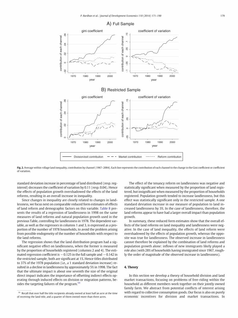
Next, we decompose the changes in inequality across the three prin-cipal channels (household division, land market transactions, and landreform) using the following accounting exercise. For each of these chan-nels, we calculate the amount of land the householdwould have ownedin any given year had the landholding change associatedwith the corre-sponding channel not occurred, and all other changes in landholdingwould have occurred as observed. We then calculate the averagewithin-village inequality that would have resulted, and subtract thisfrom the observed inequality to estimate the contribution of this chan-nel. Fig. 2 shows the results for both full and restricted samples, which

Table 6Division rates and proportion of land lost, in different size classes 1967–2004 (restrictedsample).

Land class % of households % Land lost

Landless 4.46 0.21Marginal 4.43 1.07Small 4.83 1.52Medium 4.53 1.19Large 4.19 1.04Big 5.03 1.51

Thefirst column shows the annual proportion of households that divided in a given periodof time. The second column indicates the proportion of land that households lost due todivision. Division means one or more members left the household. Numbers arepercentages.

indicate clearly that the dominant source of rising inequalitywas house-hold division, particularly after the mid-1980s. Land market transac-tions contributed to a slight increase in inequality in the restrictedsample, while reducing it in the full sample, particularly for the coeffi-cient of variation.16 The role of land reforms is comparable to that oflandmarket transactions: a slight increase in theGini coefficient and de-crease in the coefficient of variation for the full sample, while increasingthe Gini coefficient and leaving the coefficient of variation unchangedfor the restricted sample. Hence, land reforms exercised a substantiallyweaker direct effect on both the Gini coefficient and the coefficient ofvariation compared to the direct effect of household divisions.

Why the land reforms may have directly raised inequality is the fol-lowing. While the majority of those receiving land titles were landless,there were many that owned land previously. The median, 75th and90th percentile of landpreviously owned among those receiving land ti-tles (at the time of receiving the land titles) were 0.5, 3.36 and5.67 acres respectively. This indicates that there were targeting failuresin the implementation of the land distribution program, which couldpartly account for their ineffectiveness in lowering inequality.

It is conceivable, moreover, that the land reforms exerted an impor-tant indirect effect on inequality by affecting household divisions andland market transactions. A total assessment of their impact should in-corporate these indirect effects.While subsequent sectionswill treat di-visions and land transactions as endogenous, we nowpresent a reducedform estimate of the total impact of the land reform. Table 7 presentscross-village regressions predicting 1998 inequality (measured by thecoefficient of variation) by the land reforms implemented since 1968,controlling for the level of inequality in 1968 and the change in theratio of natural population in the village to cultivable land.17 The under-lying assumption is that birth and death rates were exogenous with re-spect to inequality and land reforms.18 Our control is a measure ofnatural growth of population in the village (relative to cultivable landarea) rather than of the actual population, as the latter includes possiblyendogenous effects on migration or household division.

Table 7 shows that the land title program (measured either bythe proportion of land area distributed, or proportion of households re-ceiving land titles between 1968 and 1998) registers a negative coeffi-cient, which is statistically significant in the full sample though not inthe restricted sample. The measures of tenancy reform also have a neg-ative coefficient but are statistically insignificant. On the other hand, thegrowth of natural population has a positive and significant direct effectin all specifications, highlighting the important role of this determinantof land inequality.

Based on the results in column 1, one standard deviation increase inthe index of natural population increases the coefficient of variation by0.24, while a one standard deviation increase in percentage of land dis-tributed decreases the coefficient of variation by 0.06. From the resultsin column 2, one standard deviation increase in the index of naturalpopulation increases the coefficient of variation by 0.22, while a one

16 The results do not change if we include land disposed or acquired as gift in the landmarket transaction channel.17 We obtain similar results if we use the Gini coefficient as a dependent variable.18 Results with respect to the effect of the land reforms are similar if we drop the ratio ofnatural growth of population to land as a regressor. Hence concerns with possibleendogeneity of population growth do not affect the reduced form estimate of effects ofthe land reforms.

-.02

0.0

2.0

4.0

6

cont

ribut

ion

of e

ach

chan

nel

1970 1980 1990 2000

year

-.1

-.05

0.0

5.1

.15

cont

ribut

ion

of e

ach

chan

nel

1970 1980 1990 2000

year

A) Full Sample

0.0

2.0

4.0

6

cont

ribut

ion

of e

ach

chan

nel

1970 1980 1990 2000

year

-.05

0.0

5.1

.15

cont

ribut

ion

of e

ach

chan

nel

1970 1980 1990 2000

year

B) Restricted Sample

Division/exit contribution Market contribution Reform contribution

Fig. 2.Averagewithin-village land inequality, contribution by channel (1967–2004). Each line represents the contribution of each channel to the change in theGini coefficient or coefficientof variation.


standard deviation increase in percentage of land distributed (resp. reg-istered) decreases the coefficient of variation by 0.11 (resp. 0.04). Hencethe effects of population growth overshadowed the effects of the landreforms, resulting in an overall increase in inequality.

Since changes in inequality are closely related to changes in land-lessness,we focus next on comparable reduced form estimates of effectsof land reform and demographic factors on this variable. Table 8 pre-sents the results of a regression of landlessness in 1998 on the samemeasures of land reforms and natural population growth used in theprevious Table, controlling for landlessness in 1978. The dependent var-iable, aswell as the regressors in columns 1 and 3, is expressed as a pro-portion of the number of 1978 households, to avoid the problem arisingfrom possible endogeneity of the number of households with respect tothe land reforms.

The regression shows that the land distribution program had a sig-nificant negative effect on landlessness, when the former is measuredby the proportion of households registered (columns 2 and 4). The esti-mated regression coefficient is−0.125 in the full sample and−0.142 inthe restricted sample; both are significant at 1%. Hence titles distributedto 37% of the 1978 population (i.e., a 1 standard deviation increase) re-sulted in a decline in landlessness by approximately 5% in 1998. The factthat the ultimate impact is about one seventh the size of the originaldirect impact indicates the importance of offsetting indirect effects op-erating through induced effects on division or migration patterns, be-sides the targeting failures of the program.19

19 Recall that over half the title recipients already owned at least half an acre at the timeof receiving the land title, and a quarter of them owned more than three acres.

The effect of the tenancy reform on landlessness was negative andstatistically significant when measured by the proportion of land regis-tered, but insignificantwhenmeasured by the proportion of householdsregistered. Population growth tended to increase landlessness, but thiseffect was statistically significant only in the restricted sample. A onestandard deviation increase in our measure of population to land in-creased landlessness by 3%. In the case of landlessness, therefore, theland reforms appear to have had a larger overall impact than populationgrowth.

In summary, these reduced form estimates show that the overall ef-fects of the land reforms on land inequality and landlessness were neg-ative. In the case of land inequality, the effects of land reform wereovershadowed by the effects of population growth, whereas the oppo-site was true for landlessness. The observed increase in landlessnesscannot therefore be explained by the combination of land reforms andpopulation growth alone: inflows of new immigrants likely played arole also (with 28% of households having immigrated since 1967, rough-ly the order of magnitude of the observed increase in landlessness).

4. Theory

In this section we develop a theory of household division and landmarket transactions, focusing on problems of free-riding within thehousehold as different members work together on their jointly ownedfamily farm. We abstract from potential conflicts of interest arisingwith regard to collective consumption goods. Our focus is also on purelyeconomic incentives for division and market transactions. In

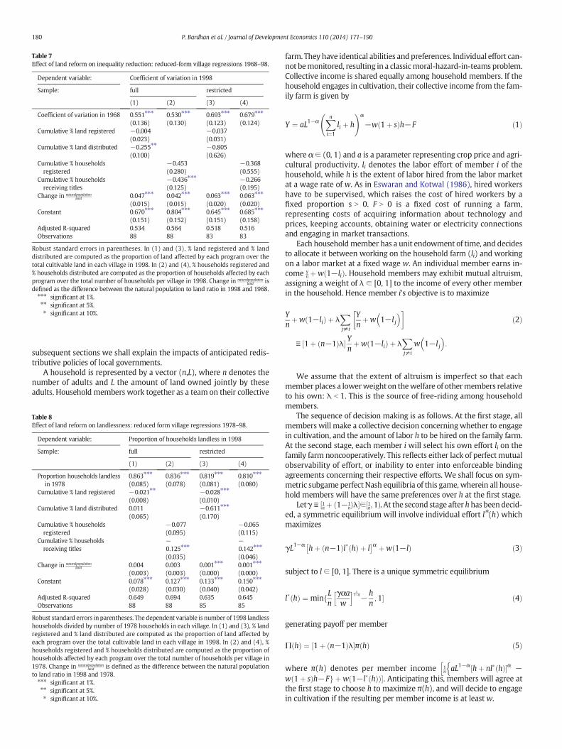
Table 7Effect of land reform on inequality reduction: reduced-form village regressions 1968–98.

Dependent variable: Coefficient of variation in 1998

Sample: full restricted

(1) (2) (3) (4)

Coefficient of variation in 1968 0.551⁎⁎⁎ 0.530⁎⁎⁎ 0.693⁎⁎⁎ 0.679⁎⁎⁎

(0.136) (0.130) (0.123) (0.124)Cumulative % land registered −0.004 −0.037

(0.023) (0.031)Cumulative % land distributed −0.255⁎⁎ −0.805

(0.100) (0.626)Cumulative % householdsregistered

−0.453 −0.368(0.280) (0.555)

Cumulative % householdsreceiving titles

−0.436⁎⁎⁎ −0.266(0.125) (0.195)

Change in naturalpopulationland 0.047⁎⁎⁎ 0.042⁎⁎⁎ 0.063⁎⁎⁎ 0.063⁎⁎⁎

(0.015) (0.015) (0.020) (0.020)Constant 0.670⁎⁎⁎ 0.804⁎⁎⁎ 0.645⁎⁎⁎ 0.685⁎⁎⁎

(0.151) (0.152) (0.151) (0.158)Adjusted R-squared 0.534 0.564 0.518 0.516Observations 88 88 83 83

Robust standard errors in parentheses. In (1) and (3), % land registered and % landdistributed are computed as the proportion of land affected by each program over thetotal cultivable land in each village in 1998. In (2) and (4), % households registered and% households distributed are computed as the proportion of households affected by eachprogram over the total number of households per village in 1998. Change in naturalpopulation

land isdefined as the difference between the natural population to land ratio in 1998 and 1968.⁎⁎⁎ significant at 1%.⁎⁎ significant at 5%.⁎ significant at 10%.


subsequent sections we shall explain the impacts of anticipated redis-tributive policies of local governments.

A household is represented by a vector (n,L), where n denotes thenumber of adults and L the amount of land owned jointly by theseadults. Household members work together as a team on their collective

Table 8Effect of land reform on landlessness: reduced form village regressions 1978–98.

Dependent variable: Proportion of households landless in 1998

Sample: full restricted

(1) (2) (3) (4)

Proportion households landlessin 1978

0.863⁎⁎⁎ 0.836⁎⁎⁎ 0.819⁎⁎⁎ 0.810⁎⁎⁎

(0.085) (0.078) (0.081) (0.080)Cumulative % land registered −0.021⁎⁎ −0.028⁎⁎⁎

(0.008) (0.010)Cumulative % land distributed 0.011 −0.611⁎⁎⁎

(0.065) (0.170)Cumulative % householdsregistered

−0.077 −0.065(0.095) (0.115)

Cumulative % householdsreceiving titles

−0.125⁎⁎⁎

−0.142⁎⁎⁎

(0.035) (0.046)Change in naturalpopulation

land 0.004 0.003 0.001⁎⁎⁎ 0.001⁎⁎⁎

(0.003) (0.003) (0.000) (0.000)Constant 0.078⁎⁎⁎ 0.127⁎⁎⁎ 0.133⁎⁎⁎ 0.150⁎⁎⁎

(0.028) (0.030) (0.040) (0.042)Adjusted R-squared 0.649 0.694 0.635 0.645Observations 88 88 85 85

Robust standard errors in parentheses. The dependent variable is number of 1998 landlesshouseholds divided by number of 1978 households in each village. In (1) and (3), % landregistered and % land distributed are computed as the proportion of land affected byeach program over the total cultivable land in each village in 1998. In (2) and (4), %households registered and % households distributed are computed as the proportion ofhouseholds affected by each program over the total number of households per village in1978. Change in naturalpopulation

land is defined as the difference between the natural populationto land ratio in 1998 and 1978.⁎⁎⁎ significant at 1%.⁎⁎ significant at 5%.⁎ significant at 10%.

farm. They have identical abilities and preferences. Individual effort can-not bemonitored, resulting in a classicmoral-hazard-in-teams problem.Collective income is shared equally among household members. If thehousehold engages in cultivation, their collective income from the fam-ily farm is given by

Y ¼ aL1−α Xni¼1

li þ h

!α

−w 1þ sð Þh−F ð1Þ

where α∈ (0, 1) and a is a parameter representing crop price and agri-cultural productivity. li denotes the labor effort of member i of thehousehold, while h is the extent of labor hired from the labor marketat a wage rate of w. As in Eswaran and Kotwal (1986), hired workershave to be supervised, which raises the cost of hired workers by afixed proportion s N 0. F N 0 is a fixed cost of running a farm,representing costs of acquiring information about technology andprices, keeping accounts, obtaining water or electricity connectionsand engaging in market transactions.

Each householdmember has a unit endowment of time, and decidesto allocate it between working on the household farm (li) and workingon a labor market at a fixed wage w. An individual member earns in-come Y

n þw 1−lið Þ. Household members may exhibit mutual altruism,assigning a weight of λ ∈ [0, 1] to the income of every other memberin the household. Hence member i's objective is to maximize

Ynþw 1−lið Þ þ λ

Xj≠i

Ynþw 1−l j

� ��

≡ 1þ n−1ð Þλ½ � Ynþw 1−lið Þ þ λ

Xj≠i

w 1−l j� �

:

ð2Þ

We assume that the extent of altruism is imperfect so that eachmember places a lowerweight on thewelfare of othermembers relativeto his own: λ b 1. This is the source of free-riding among householdmembers.

The sequence of decision making is as follows. At the first stage, allmembers will make a collective decision concerningwhether to engagein cultivation, and the amount of labor h to be hired on the family farm.At the second stage, each member i will select his own effort li on thefamily farm noncooperatively. This reflects either lack of perfect mutualobservability of effort, or inability to enter into enforceable bindingagreements concerning their respective efforts. We shall focus on sym-metric subgame perfect Nash equilibria of this game, wherein all house-hold members will have the same preferences over h at the first stage.

Letγ ≡ 1n þ 1−1

nð Þλ½ �∈½1n;1Þ. At the second stage after hhas been decid-ed, a symmetric equilibrium will involve individual effort l⁎(h) whichmaximizes

γL1−α hþ n−1ð Þl� hð Þ þ l� �α þw 1−lð Þ ð3Þ

subject to l ∈ [0, 1]. There is a unique symmetric equilibrium

l� hð Þ ¼ minfLn

γαaw

h i 11−α− h

n;1� ð4Þ

generating payoff per member

Π hð Þ ¼ 1þ n−1ð Þλ½ �π hð Þ ð5Þ

where π(h) denotes per member income 1n aL1−α hþ nl� hð Þ½ �αnh

−w 1þ sð Þh−Fg þw 1−l� hð Þð Þ�. Anticipating this, members will agree atthe first stage to choose h to maximize π(h), and will decide to engagein cultivation if the resulting per member income is at least w.


In what follows we shall focus on situations where there is enoughaltruism within households, so that

λN1

1þ s: ð6Þ

This assumption is relatively inessential as qualitatively similar re-sults also obtainwhen it does not hold, though the detailed results differin that case.20When Eq. (6) holds, (1+ s)γ N 1, irrespective of the valueof n. We can then classify households into three types on the basis oftheir endowment of land relative to household members:

(a) land-poorwhere

Lnb

wγαa

� � 11−α ð7Þ

(b) medium-land where

wγαa

� � 11−α

≤ Ln≤ w 1þ sð Þ

αa

� � 11−α ð8Þ

(c) land-richwhere

LnN

w 1þ sð Þαa

� � 11−α

: ð9Þ

The following Proposition describes the nature of the uniquesymmetric equilibrium.

Proposition 1. Assume that Eq. (6) holds.

(i) Conditional on deciding to cultivate, a symmetric equilibriumresults in the following:(a) For land-poor households: l� ¼ L

nγαaw½ � 1

1−α b1; h� ¼ 0 and permember income of

πp ≡1n

La1

1−αw−α1−α γαð Þ α

1−α− γαð Þ 11−α

n o−F

h iþw: ð10Þ

(b) For medium-land households: l∗ = 1, h∗ = 0 and eachmember earns

πm ≡ 1n

aL1−αnα−Fh i

: ð11Þ

(c) For land-rich households: l� ¼ 1;h� ¼ L aαw 1þsð Þ

h i 11−α−n and each

member earns

πr ≡1n

La1

1−α w 1þ sð Þf g−α1−α α

α1−α−α

11−α

n o−F

h iþw 1þ sð Þ: ð12Þ

(ii) The household decides not to cultivate if the resulting incomepermember falls below w, i.e. for land-poor households if:

L b L�p ≡ Fa−11−αw

α1−α γαð Þ α

1−α− γαð Þ 11−α

h i−1; ð13Þ

for medium-land households if:

L b L�m ≡ F þ nwð Þa−1n−αh i 1

1−α; ð14Þ

and land-rich households if:

L b L�r ≡ F−nws½ �a −11−α w 1þ sð Þ½ � α

1−α αα

1−α−α1

1−α

h i−1: ð15Þ

20 Themain difference when Eq. (6) does not hold is that there may be two types of cul-tivating households rather than three: themedium-land type of householdmay not arise.

(iii) There is free-riding (i.e., member incomes are not maximized)only in land-poor households.

Proof of Proposition 1. Given h, a symmetric equilibrium effort l∗(h) atthe second stagemust maximize γaL1 − α((n− 1)l∗ + l+ h)α+w(1−l) with respect to choice of l∈ [0, 1]. Hence l� hð Þ ¼ min L

nγαaw

� 11−α−h

n;1n o

.

This implies that aggregate labor hours in the household farm l hð Þ ≡nl� hð Þ þ h ¼ min L γαa

wð Þ 11−α;nþ h

n o.

The first-stage choice of h will then maximize aL1 − αl(h)α −w(1 + s)h subject to h≥ 0. Given the expression for l(h) above, it is ev-ident that the optimal choice of h∗ N 0 only if L γαa

wð Þ 11−α ≥nþ h, which im-

plies that l∗(h) = 1 and l(h) = n + h. Then h∗ N 0 if and only ifcondition (12) holds, i.e., the household is land-rich. In that case wealso have l∗ = 1.

If condition (12) does not hold, either Eq. (10) or (11) holds. Wehave h∗=0 for these households. Evidently the equilibriummember ef-fort l∗ = l∗(0) b 1 if Eq. (10) holds, while l∗ = l∗(0) = 1 if Eq. (11) holds.The rest of Proposition 1 follows from routine computations. ■

Land-poor households have ‘surplus labor’: they divide time be-tween working on the family farm and on the outside market. Noworkers are hired from themarket. Owing to imperfect altruism, mem-bers spend too little timeon the family farm. Incomepermemberwouldbe maximized if each member were to supply labor of L

nαaw½ � 1

1−α on theirown farm, which is larger than what they actually supply (sinceγ N 1). In households that are not land-poor, members work full timeon the family farm and there is no free-riding: the equilibrium maxi-mizes income per member. Medium-land households rely entirely onthe labor of its members. Land-rich households encounter enoughlabor scarcity that it is worthwhile for them to hire workers from themarket. These land-rich households constitute the employers on thelabor market.

For households of any given type, they decide to operate a familyfarm only if they own aminimum amount of land, given by expressionsLp∗ , Lm∗ and Lr

∗ for the three types respectively. A minimum landholding isnecessary to ensure that the household earns enough from the farm tocover its fixed costs. Those owning less land would not operate a farmand rely entirely on supplying labor to other farms. The supply side ofthe labor market is constituted of such land-poor households.

The model could be closed with wage rates determined by the con-dition that the labor market clears. In what follows we shall abstractfrom the possibility of equilibrium wages that respond to village levelshocks. We assume that there is a sufficiently large mass of landlesshouseholds in the village, which pins wages down to an exogenouslyfixed reservation wage for the landless. The justification for this is em-pirical:we donot see significant responses ofwage rates to land reformsin West Bengal (Bardhan and Mookherjee, 2011, Table 14). And as weshall see below, there is a large and growing mass of landless house-holds in these villages, supplemented by inflows of immigrants.

4.1. Household division

We now discuss how the equilibrium described in Proposition 1would be modified if households could sub-divide. To start with we ab-stract from the possibility of a land market; the next section will de-scribe the consequences of introducing such a market.

A household is described by its size and landholding (n,L) which en-ables its members to earn an income ofΠ(n,L) from a household collec-tive farm. This can be viewed as the short-run outcome. Over time, thehousehold can experience change in a variety of ways. Some membersmay exit, or the household may divide into two smaller households.

Some members could quit while others remain in cultivation: callthis exit or out-migration. An extreme case of this is when every mem-ber of the household decides to quit and go to work full time on thelabor market. This is essentially the counterpart of deciding to not


cultivate a family farm at all. Call this a shutdown. Finally, the householdcould divide into two cultivating households, which we shall refer to asdivision.

More complicated changes may involve a combination of exit anddivision, or a division of the household into more than two households.We shall ignore this for the time being, as it can be shown it suffices toconsider these three kinds of changes to describe stable householdstructures.

An important assumption we make is that two households cannotmerge into a single large household. The incentive for a merger couldarise from avoiding the duplication of the fixed costs of farming. Thisphenomenon is empirically very rare, possibly for the reason thathouseholds are formed around close kinship and familial ties. If thevillage is partitioned into ‘familial’ subsets of individuals with highaltruismwithin subsets and low altruismacross subsets, coalitions com-prising individuals from disparate ‘families’would encounter too muchfree-riding andwould thereby not be stable. In that case households canonly be subsets of families. We have in mind an initial situation wherehouseholds are of maximal size within each family, and are subject todivision pressures owing to growth in household size owing to demo-graphic reasons. We abstract from this complication by simply exclud-ing the possibility of mergers.

We make additional simplifying assumptions of transferable utilityand symmetric information within each household. So exits and divi-sions can be accompanied by side-transfers among members — e.g.,exiting members can be given a side-transfer by remaining members.Under this assumption, exits and divisions will take place if and only ifthe total income ofmembers of the original household increases as a re-sult. This motivates the following definition.

Definition 1. A cultivating household (n,L) is stable if its members donot collectively benefit from a shutdown, exit or division:

Π n; Lð Þ≥w ðNSÞ

nΠ n; Lð Þ≥mwþ n−mð ÞΠ n−m; Lð Þ for any m∈ 1;…;n−1f g ðNEÞ

nΠ n; Lð Þ≥n1Π n1; L1ð Þ þ n−n1ð ÞΠ n−n1; L−L1ð Þfor any L1bL; and any n1∈ 1;…;n−1f g:

ðNDÞ

Conversely it is unstable if one or more of these inequalities areviolated.

It may be argued that condition (NE) is incorrect if the householdthat remains after the exit of m members is induced to shut down(which will happen ifΠ(n−m, L) b w), since the payoff of the remain-ing members would then equal w rather than Π(n − m, L). But in thiscase the consequences of exit would be the same as shutdown, so thiscase is covered by (NS). Similarly, in the case of division where Π(n1,L1) b w, but it pays the remaining household to continue to cultivate,the correct condition should be nΠ(n, L) ≥ n1w + (n − n1)Π(n − n1,L − L1). Since Π is increasing in L, this condition is ensured by (NE).21

21 Nevertheless, theremay still be the concern that the notion of stability could fail a con-sistency condition: e.g., one of the fragmented households may itself be unstable andprone to further exits or divisions, which members of the original household ought to an-ticipate. However, this will not be a problem since further exits or divisions of one of thefragments would only serve to increase further the collective payoff of the members ofthat fragment. So conditions (NS), (NE) and (ND) are necessary for stability. Are they suf-ficient? In other words, what about the possibility of division into three or more house-holds, or combinations of exits and division? This is not a problem for the followingreason. Owing to the assumption concerning presence of fixed costs and CRS technology,a household dividing into two ormore fragmentswill not be able to attain a higher collec-tive profit. Hence the three conditions are collectively sufficient.

In the absence of a land market and given the assumption of exoge-nouswages, the stability of a household is independent of the character-istics of other households in the village. Hence we can define a stablehousehold distribution as follows. We shall refer to any household(n,L) as a cultivating household if Π(n, L) ≥ w, and a non-cultivatinghousehold otherwise. A non-cultivating household does not utilize itsland: such a household might gift its land to other cultivating house-holds, or sell it if there is a landmarket. Sowithout any loss of generalitywe can identify non-cultivating households as landless.

Definition 2. A distribution over households (i.e. vectors (n,L)) is stableif there is no positive fraction of cultivating households that are unsta-ble. Otherwise it is said to be an unstable distribution.

Our main result below provides a near-complete characterization ofthe set of stable cultivating households.

Proposition 2. A cultivating household (n,L) is stable if there is no free-riding and each member earns at least w, i.e., the following conditionshold:

L≥LI nð Þ≡ n λþ 1n

1−λð Þ� � −1

1−α waα

� � 11−α ðICÞ

L≥LR nð Þ ðIRÞ

where LR(n) equals Lp∗ , Lm∗ , Lr∗ for land-poor, medium-land and land-richhouseholds respectively (as defined in Proposition 1).

Conversely, the household is unstable if it violates either (IR) or

nN ⌊nI Lð Þ⌋ ðIC′Þ

where nI(L) denotes the inverse of LI(n) and ⌊x⌋ denotes the smallest in-teger exceeding x.

Proof of Proposition 2. We start with sufficiency. Suppose there is nofree-riding and each member earns at least w. The latter implies that(NS) is satisfied. To show (NE) holds, note that LI(n) is an increasingfunction. So for any positive integer m, the equilibrium outcome for ahousehold with n–m members and L land will involve no free-riding,with eachmember selecting l=1. This implies that themarginal contri-bution of any member in any such household exceeds w, and so themarginal contribution of m members will exceed mw, which implies(NE). (ND) follows from noting that the production function definedby ‘output’ equal to collective income of a household plus the fixedcost, and inputs consisting of land L and household size n (i.e., y(L, n)which equals nπm + F for a medium-land household and nπr + F for aland-rich household) defines a production set which is a convex cone.Hence the collective income of the household net of the fixed cost issuperadditive. ■

The necessity of (IR) for stability is obvious. To shownecessity of (IC′),suppose this condition is violated and we have n N ⌊nI(L)⌋. This impliesthat there is free riding at both n and n-1, and per member incomesare defined by Eq. (10). Hence nπp(n, L) = nw − F + H(n) and (n −1)πp(n − 1, L) = (n − 1)w − F + H(n − 1) whereH mð Þ≡ La 1

1−αw−α1−α

γ mð Þαð Þ α1−α− γ mð Þαð Þ 1

1−al

n oand γ mð Þ≡ λþ 1−λð Þ1m . Clearly γ(m) is

strictly decreasing in m. Hence nπp(n, L) − (n − 1)πp(n − 1, L) =w + H(n) − H(n − 1) b w, and (NE) is violated. ■

Proposition 2 is illustrated in Fig. 3. (IC) is an incentive compatibilitycondition, stating that given the land owned by the household, thenumber of members is small enough to ensure absence of free-riding:every member supplies maximal effort in the farm. It is a restatementof the condition that the household be either medium-land or land-rich. The corresponding necessary condition (IC′) is slightly weaker,owing to the fact that the number of household members is integer-

22 For the same reason, division into three or more fragments would not be valuable,when it is not worthwhile to fragment into two fragments.23 Suppose the IC constraint is the first one that is violated, with n close enough to nI(L)after the demographic expansion, and fixed costs F smaller thanw. Then had the originalhousehold remained intact themarginal contribution of anymember to collective incomewill be at leastw. Hence the exit of anymemberwould result in a reduction in total incomeby at leastw. On the other hand, it is feasible to divide the household into two cultivatinghouseholdswhich are stable, inwhich case their collective incomewill decline by F, whichis smaller than w. In this case division is going to happen rather than exit. On the otherhand, if F is large enough then exit will happen rather than division.

Fig. 3. Characterization of stable households without landmarket transactions. Stable areas are depicted in light gray. Area 1 is characterized by no free-riding (l∗=1), positive hired labor(h∗ N 0) and income increases in family size Y′(n) N 0. In area 2 there is no free-riding (l∗=1), nohired labor (h∗=0), and income increaseswith family size (Y′ N 0). Finally, in area 3 thereis free-riding (l∗ b 1), no hired labor (h∗ = 0), and income does not increase with family size (Y′= 0).


valued. The necessity of this condition flows from the fact that land-poor households are characterized by free-riding, and collective house-hold income is strictly decreasing in the number of members. It thenpays one member to exit with a suitable compensation paid by the re-maining household members. Condition (IC) reduces to a minimumlandholding requirement LI(n) which is strictly increasing and strictlyconvex in household size n, provided the extent of altruism is imperfect(i.e., λ b 1). Conversely it amounts to a maximum household size nI(L)corresponding to any given ownership of land.

The existence of a limit to household size arises due to the assump-tion that altruism within the household is not perfect. If instead λ = 1,therewould never be any free-ridingwithin the household, and the col-lective income of the household would be independent of householdsize within region (a). The condition for the household to be stable isthat L a aα

w½ � α1−α−w aα

w½ � 11−α

n oN F , which does not depend on household size.

As household size increases, its members would spend proportionatelyless time per capita working on the household farm, and more time onthe labor market. The total amount of labor on the family farm, andhence the collective income realized from it would be unchanged. Aslong as the collective income is greater than the fixed cost, the farmwould be operational and the household would face no compulsion tosplit or for its members to leave.

Returning now to the case with imperfect altruism, condition (IR) isan individual rationality constraint that corresponds to condition (NS)wherein every member should earn at least as what they would earnon their own working full time on the labor market. It translates into aminimum landholding requirement LR(n) given household size. It is ev-ident that for land-rich households this lower bound Lr(n) is linear anddecreasing in n. For medium-land households, the bound Lm(n) is U-shaped in n, achieving a minimum at n� ¼ α

1−αFw. Since stability also re-

quires ‘near-absence’ of free-riding within the household as expressedby condition (IC′), Lm(n∗) forms an approximate lower bound to thelandholding of any stable household, irrespective of how many mem-bers it has. Hence a stable land distribution must exhibit a ‘hole’ in-between 0 and Lm(n∗) quantities of land. Note also that the minimumlandholding size needed to satisfy (IR) depends on both F and w. Evenif F were zero, a minimum land size would be needed to ensure thatper capita earnings are above the wage rate.

The sufficiency of the two conditions arise from the fact that a non-land-poor household realizes maximal agricultural income from its en-dowment of labor and land, which is increasing in n and L. The absenceof free-riding in such households implies that themarginal contributionof each member to household income exceeds the outside wage w.Hence there are no incentives for exit. There are no incentives for divi-sion either— at best the fragmentswould be better off cultivating ratherthan not cultivating (whichwould happen if they both continued to sat-isfy (IR)). And the best-case scenario for division is when neither frag-ment is characterized by any free-riding. In that case owing to theconstant returns feature of the production function (ignoring the fixedcost), collective production would remain the same, and collective

income would decline on account of the duplication of fixed cost F.22

Finally, the (IR) constraint implies that there are no benefits fromshutdown.

It is easy to check that the IC and IR curves cross in the n–L space at asingle point n∗∗. To the right (left) of this, the IC curve lies above (resp.below) the IR curve. In case A of Fig. 3 where F

w is high enough (relativeto α), they intersect to the right of the bottom of the IR curve (i.e.,n∗∗ N n∗). In the other Case B when F

w is low, they intersect to the left ofthe bottom (n∗∗ N n∗). The implications of the demographic growth ofthe number of household members can differ between the two cases,as we discuss next.

4.2. Effects of changes in demographics and profitability on the landdistribution

Suppose we start with a stable distribution, with the support of cul-tivating households contained in the region bounded below by the in-tersection of the IR and IC curves, with all remaining householdslandless. Now take any cultivating household which is initially in thestable region, and suppose that the number of household members in-creases (owing to either fertility increases or decreases in mortality)while its landholding remains the same.

Consider case B of Fig. 3, with relatively low fixed costs. Or supposewe are in case A instead, but n exceeds n∗. If the number of members in-creases sufficiently, the IC constraint will be violated and the householdwill cease to be stable. As the endowment point moves across the ICcurve, the IR constraint continues to be satisfied. Hence either exit or di-vision of the household will be induced, rather than a shutdown. Theproblem is that the household has too many members relative to itsland, inducing some free-riding.

It is also possible that the IR constraint is the first to be violated as thehousehold size grows relative to its landholding. Thiswouldhappen for in-stance in Case Awhere the landholding is close to the lower bound Lm(n∗).

Can we predict whether the outcome of demographic growth willbe exit (in which case n will fall while L of the surviving householdwill remain unchanged) or division (whence landholdings of the sur-viving fragments will be smaller than that of the original house-hold)? Which of these two outcomes will happen will depend onwhich is associated with a higher collective income of the membersof the original household.23 Note that exit is always feasible, since


the extra number of household members that caused IC to fail canexit so as to leave a cultivating household with exactly the samenumber of members as in the original household. But division maynot be feasible, if there was little slack in the IR constraint to startwith. For instance, division is infeasible if the original householdowned less than twice Lm(n∗), since each of the fragments will haveto have at least this amount of land in order to be viable. At thelower end of the land distribution, thus, demographic growthwill re-sult in exits, resulting in growing landlessness.

Next suppose agricultural profitability (represented by aw) increases.

This causes the IC curve to shift outwards, and the IR curve movesdownwards — both constraints are relaxed. This will tend to slowdown exits and divisions occurring due to demographic growth.

4.3. Land market transactions

Now suppose that land can be bought and sold, subject to a unittransaction cost of t. Other problems that may restrict land markettransactions include credit constraints that restrict purchases, status ef-fects or insurance value of land that make households reluctant to sell.Asymmetric information concerning land quality may also create a‘market for lemons’ problem. We abstract from these here, and focuson the role of costs of registering land transactions.

Continuing with the assumption of transferable utility and lack ofcredit constraints or asymmetric information, two cultivating house-holds (ni, Li), i=1, 2 will have an incentive to engage in a land transac-tion of l units if and only if

n1Π n1; L1−lð Þ þ n2Π n2; L2 þ lð Þ−tlNn1Π n1; L1ð Þ þ n2Π n2; L2ð Þ:

Since the marginal contribution of land to collective income of anymedium-land household (n, L) equals 1−αð Þa n

Lð Þα , it follows that thereis an incentive for two medium-land households to enter into a landtransaction if and only if their relative endowments differ sufficiently,relative to transaction costs and profitability parameter a:

j n1

L1

�α− n2

L2

�αjN t

a 1−αð Þ : ð16Þ

The results in the preceding section imply that in order to identifystable land distributions, we can focus on households that are eitherland-rich or medium land types. All land-rich households have thesame marginal value of land, equal to the value of land for a medium-land household located at the boundary between the medium-land

and land-rich regions, i.e., with nL ¼ b≡ αa

w 1þsð Þ

n o 11−α

. For purposes of land

transactions we can identify land-rich households with such amedium-land household.

The definition of a stable land distribution must now include thecondition that no two cultivating households should want to enterinto a profitable land transaction.24 This restricts the range of variationof factor proportions among all cultivating households (after settingthe factor proportion of land-rich households to b) to lie within a coneof width which varies with t

a 1−αð Þ, as shown in Fig. 4. The stable region,i.e., support of a stable land distribution (for cultivating households)must now be contained within the intersection of such a cone with

24 We ignore the possibility of purchases of land by landless households from cultivatinghouseholds. Such transactions are empirically rare. Possible reasons include a large fixedcost F of operating a farm. These necessitate a large amount purchase of land by the land-less, which they may be unable to finance owing to credit constraints. Moreover thesefixed costs would be duplicated, eroding the potential benefits of the transaction: itwouldnot be profitable if F is sufficiently large relative tow. Additional complications arise whenwe consider possible combinations of exits or divisions with land market transactions, sowe stop short of providing a characterization of stable land distributions and instead focuson necessary conditions.

the areas bounded below by the IC and IR curves. If t is small, thiscone may be contained entirely within the medium-land region. Inthat case there is a stable distribution containing only medium-landhouseholds. For the same value of t, there could be multiple cones con-sistent with the stability condition: there could be another cone whichincludes the factor proportion b and other medium-land householdsin the interior of the medium-land region. In this case a stable distribu-tion could include both medium-land and land-rich types of house-holds. Note in particular that for any t there exists a stable distributioncontaining only land-rich households, as there are no incentives forany pair of land-rich households to trade land.

Demographic growth in some households may now trigger a landtransaction rather than an exit or division. This is shown in Fig. 4(B),where a household with a relatively high initial ratio of labor to land(represented by vector h) moves to h1. It then enters into a land pur-chase from another household h2 with a relatively low labor–landratio, with respect to whom condition (16) is now violated. As a resultof the transaction, h1 moves up back to h3 into the equilibrium cone,while h2 drops down to h4 and continues to remain in the stable region.Clearly, the likelihood of buying land is increasing in n

L and in a, while thelikelihood of selling land is decreasing in n

L and increasing in a.

5. Regression analysis results for household division, landtransactions and immigration

We now test the predictions of the preceding model with regard tothe determinants of household division and land transactions. Follow-ing the discussion of determinants of household division above, weuse the following regression specification:

DIVivt ¼ βi þ δt þ β1HSi;t−1 þ β2Li;t−1 þ β3TRv;t−k þ β4TRv;t−k � Li;t−1þ β4LDv;t−k þ β5LDv;t−k � Li;t−1 þ β6Cit þ ϵivt

ð17Þ

where DIVivt denotes a dummy for division, or land lost owing to divi-sion, by household i located in village v in year t. The regressors includeapart from household fixed effects and year effects, lagged householdsize HS, landownership L, measures of implementation of the tenancyreform TR and the land distribution program LD in the village laggedby a few (k) years,25 interactions of these with lagged land owned bythe household, and a dummy C for whether the household ownedland in excess of the legal ceiling. We report both logit and linear prob-ability versions of this regression. Standard errors of residuals ϵivt areclustered at the village level.

We also use a similar specification to analyze whether a householdbought or sold land. The theory indicated that the likelihood of buyingor selling would be related to the ratio of (lagged) household size toland owned, so we include a specification where the log of this ratio isused as a single regressor apart from household and time effects. Thiscorresponds to a different functional form, representing differences inendowment compositions that motivate land market transactions.

5.1. Regression results for household division

Table 9 presents a logit regression predicting the event that a house-hold experienced a division in any given year. Columns1 through3 showthe results for the full sample and 4 through 6 for the restricted sample.Columns 3 and 6 present the specification described above, withthe other columns showing a more parsimonious specification whichdrops some of the land reform variables and some interaction terms.

Focusing on columns 3 and 6, we find that growth in householdsize significantly raised the likelihood of household division. This con-firms the notion that demographic growth was a key determinant ofdivision — households with more family members were more likely

25 We take the sum of these in three preceding years.

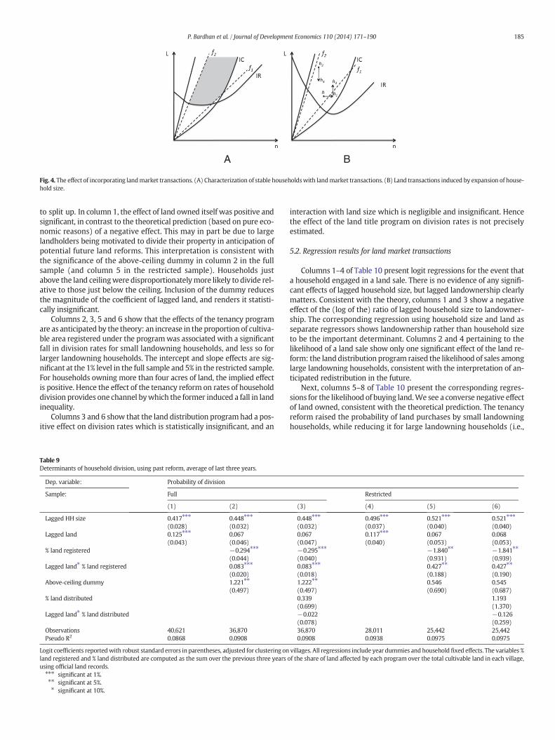
BA

Fig. 4. The effect of incorporating landmarket transactions. (A) Characterization of stable householdswith landmarket transactions. (B) Land transactions induced by expansion of house-hold size.


to split up. In column 1, the effect of land owned itself was positive andsignificant, in contrast to the theoretical prediction (based on pure eco-nomic reasons) of a negative effect. This may in part be due to largelandholders being motivated to divide their property in anticipation ofpotential future land reforms. This interpretation is consistent withthe significance of the above-ceiling dummy in column 2 in the fullsample (and column 5 in the restricted sample). Households justabove the land ceilingwere disproportionatelymore likely to divide rel-ative to those just below the ceiling. Inclusion of the dummy reducesthe magnitude of the coefficient of lagged land, and renders it statisti-cally insignificant.

Columns 2, 3, 5 and 6 show that the effects of the tenancy programare as anticipated by the theory: an increase in the proportion of cultiva-ble area registered under the programwas associated with a significantfall in division rates for small landowning households, and less so forlarger landowning households. The intercept and slope effects are sig-nificant at the 1% level in the full sample and 5% in the restricted sample.For households owning more than four acres of land, the implied effectis positive. Hence the effect of the tenancy reform on rates of householddivision provides one channel bywhich the former induced a fall in landinequality.

Columns 3 and 6 show that the land distribution programhad a pos-itive effect on division rates which is statistically insignificant, and an

Table 9Determinants of household division, using past reform, average of last three years.

Dep. variable: Probability of division

Sample: Full

(1) (2)

Lagged HH size 0.417⁎⁎⁎ 0.448⁎⁎⁎

(0.028) (0.032)Lagged land 0.125⁎⁎⁎ 0.067

(0.043) (0.046)% land registered −0.294⁎⁎⁎

(0.044)Lagged land⁎ % land registered 0.083⁎⁎⁎

(0.020)Above-ceiling dummy 1.221⁎⁎

(0.497)% land distributed

Lagged land⁎ % land distributed

Observations 40,621 36,870Pseudo R2 0.0868 0.0908

Logit coefficients reportedwith robust standard errors in parentheses, adjusted for clustering onland registered and % land distributed are computed as the sum over the previous three yearsusing official land records.⁎⁎⁎ significant at 1%.⁎⁎ significant at 5%.⁎ significant at 10%.

interaction with land size which is negligible and insignificant. Hencethe effect of the land title program on division rates is not preciselyestimated.

5.2. Regression results for land market transactions

Columns 1–4 of Table 10 present logit regressions for the event thata household engaged in a land sale. There is no evidence of any signifi-cant effects of lagged household size, but lagged landownership clearlymatters. Consistent with the theory, columns 1 and 3 show a negativeeffect of the (log of the) ratio of lagged household size to landowner-ship. The corresponding regression using household size and land asseparate regressors shows landownership rather than household sizeto be the important determinant. Columns 2 and 4 pertaining to thelikelihood of a land sale show only one significant effect of the land re-form: the landdistribution program raised the likelihood of sales amonglarge landowning households, consistent with the interpretation of an-ticipated redistribution in the future.

Next, columns 5–8 of Table 10 present the corresponding regres-sions for the likelihood of buying land.We see a converse negative effectof land owned, consistent with the theoretical prediction. The tenancyreform raised the probability of land purchases by small landowninghouseholds, while reducing it for large landowning households (i.e.,

Restricted

(3) (4) (5) (6)

0.448⁎⁎⁎ 0.496⁎⁎⁎ 0.521⁎⁎⁎ 0.521⁎⁎⁎

(0.032) (0.037) (0.040) (0.040)0.067 0.117⁎⁎⁎ 0.067 0.068(0.047) (0.040) (0.053) (0.053)−0.295⁎⁎⁎ −1.840⁎⁎ −1.841⁎⁎

(0.040) (0.931) (0.939)0.083⁎⁎⁎ 0.427⁎⁎ 0.427⁎⁎

(0.018) (0.188) (0.190)1.222⁎⁎ 0.546 0.545(0.497) (0.690) (0.687)0.339 1.193(0.699) (1.370)−0.022 −0.126(0.078) (0.259)36,870 28,011 25,442 25,4420.0908 0.0938 0.0975 0.0975

villages. All regressions include year dummies and household fixed effects. The variables %of the share of land affected by each program over the total cultivable land in each village,

Table 10Determinants of land sales and purchases, using lagged land reform, average for past 3 years.

Dep. variable: Pr (land sale) Pr (land purchase)

Sample: Full Restricted Full Restricted

(1) (2) (3) (4) (5) (6) (7) (8)

log Lagged HH SizeLagged land

� �−0.908⁎⁎⁎ −1.086⁎⁎⁎ 0.063⁎⁎ 0.054(0.184) (0.161) (0.028) (0.036)

Lagged HH Size 0.035 −0.018 0.013 −0.010(0.043) (0.050) (0.038) (0.048)

Lagged land 0.133⁎⁎ 0.480⁎⁎⁎ −0.252⁎⁎⁎ −0.228⁎⁎⁎

(0.056) (0.077) (0.052) (0.057)% land registered 0.163 −0.002 0.503⁎⁎⁎ 0.510⁎⁎⁎

(0.594) (0.891) (0.072) (0.058)Lagged land⁎ % land registered −0.153 −0.094 −0.132⁎⁎ −0.153⁎⁎⁎

(0.267) (0.405) (0.053) (0.043)% land distributed −1.776 −3.220 −1.904 −0.278

(1.760) (3.839) (1.422) (3.184)Lagged land⁎ % land distributed 0.697⁎⁎ 0.833 0.739⁎⁎⁎ 0.082

(0.309) (0.711) (0.260) (0.916)Above-ceiling dummy 0.311 0.354 0.924⁎⁎ −0.004

(0.351) (0.450) (0.471) (0.538)Observations 12,612 11,483 8623 7837 10,438 9546 6952 6339Pseudo R2 0.0639 0.0511 0.0805 0.0824 0.0394 0.0519 0.0459 0.0573

Logit coefficients reportedwith robust standard errors in parentheses, adjusted for clustering on villages. Regressions include household fixed effects and year dummies. % land registeredand % land distributed are computed as the sum over the previous three years of the share of land affected by each program over the total cultivable land in each village.⁎⁎⁎ significant at 1%.⁎⁎ significant at 5%.⁎ significant at 10%.

Table 11Determinants of immigration, cross section 1978–98.

Dependent variable: Proportion of post-1967 immigrant households in 1998

Sample Full Restricted

(1) (2) (3) (4)

Cumulative % land registered −0.004 −0.002(0.015) (0.016)

Cumulative % land distributed 0.175⁎⁎⁎ 0.581⁎⁎

(0.069) (0.204)Cumulative %

households registered−0.168 −0.138(0.146) (0.209)

Cumulative %households distributed

0.095 0.108(0.076) (0.083)

Land per capita −0.158⁎⁎⁎ −0.164⁎⁎⁎ −0.192⁎⁎⁎ −0.190⁎⁎⁎

(0.066) (0.071) (0.079) (0.082)Constant 0.238⁎⁎ 0.245⁎⁎ 0.260⁎⁎ 0.281⁎⁎

(0.033) (0.033) (0.034) (0.037)Observations 89 89 88 88Adjusted R-squared 0.067 0.031 0.095 0.029

Robust standard errors in parentheses. In (1) and (3), % land registered and % landdistributed are computed as the proportion of land affected by each program over thetotal cultivable land in each village. In (2) and (4), % households registered and %households distributed are computed as the proportion of households affected by eachprogram over the total number of 1978 households per village. Land per capita is theratio of cultivable land to village population in 1978. All measures of land registrationand land distribution are computed on the basis of official land records⁎⁎⁎ significant at 1%.⁎⁎ significant at 5%.⁎ significant at 10%.


those owning more than five acres). The land distribution program hassignificant effects only in the full sample, where it attenuated the reduc-tion in the probability of purchase by large landowners. However thislast result is not robust to the choice of sample. These results, as wellas those for land sales, are unaffected by including land disposed or ac-quired as gift together with land market transactions.

In summary, the evidence shows that the land reforms inducedgreater activity in the land market. And effects of the tenancy reformon market transactions – raising (resp. lowering) the likelihood ofsmall (resp. large) landowners buying land – also constituted a channelby which they indirectly induced a drop in inequality. As in the case ofeffects on divisions, we are unable to obtain a precise estimate of the ef-fects of the land title distribution program.

5.3. Regression results for immigration

Table 11 considers the determinants of the arrival of immigrants intothese villages. It regresses the proportion of 1998 households that im-migrated into the village since 1967, on the extent of land reforms im-plemented since 1968, controlling for land per capita in 1968. There isa significant negative coefficient on land availability, possibly reflectinga greater tendency for immigrants to settle in areas of high populationdensity (owing to their concern for finding employment as workers).Moreover, immigrants were more inclined to arrive in those villagesin which more land was distributed through land reforms. The othermeasures of land reform have statistically insignificant effects.

This shows one important channel by which the land distributionprogram exerted a negative indirect effect on inequality, and a positiveeffect on landlessness.

5.4. Robustness: instrumental variable estimates for household division

One possible concern with the preceding section is that im-plementation rates may be correlated with time-varying village-level unobservables that affect division rates, which would lead toan endogeneity problem. We now address this concern with a corre-sponding instrumental variable estimator of the effect of the tenancyreform on the likelihood of household division.

To instrument for tenancy reform, we exploit the fact that thereare political economy determinants of reforms that are plausiblyuncorrelated with other factors that would affect division rates. Webase our instruments on (Bardhan and Mookherjee (2010)), whichare also used as instruments for the tenancy program implementationrate in Bardhan and Mookherjee (2011). Bardhan and Mookherjee's(2010) analysis of the political economy of the land reforms arguedthat political competition between the Left Front (LF) and the IndianNational Congress (INC), the two principal competing parties in WestBengal politics, played an important role in determining local imple-mentation rates. This gives rise to an inverted-U relationship between

28 Unfortunately, we have not succeeded in finding a set of instruments that can helppredict land distribution implementation, so we cannot test for endogeneity bias with re-gard to that program specifically.29 Native village population grew by 22% between 1978 and 1998, using the number ofvillage households from the indirect survey in Bardhan and Mookherjee (2006, 2010)and the average household sizes in these two years from the direct household survey. Ap-plied to amean household size of 5.7 in 1978, this implies that household size would haveexpanded by approximately 1.3 members, in the absence of any division.30 From column 2, the coefficient with respect to lagged household size is .103, whichmultiplied by 1.3 yields .134. The coefficient with respect to tenancy registration is− .069, which multiplied by the cumulative proportion of area registered of .11 yields− .008.31 Similar results are obtained upon using the results of the logit specification. The mar-ginal effects implied by Table 9 in the restricted sample (averaged across all households,with fixed effects set at zero) of household size was .043, of tenancy registration was− .123 and that of the land title program was .09. While the effect of household size issmaller than that in the linear probability specification, the effects of the two land reformprograms run in opposite directions and thus neutralize each other. This implies thatadding 1.3 members to household size would imply a rise in division rates by approxi-


reform implementation rate and the proportion of local governmentseats secured by the LF in the previous election, with a peak locatedaround 50%. Moreover, in villages where one of the two parties, saythe LF, was already strongly entrenched (as indicated by a share of theLF in the current local government seats that significantly exceeded50%), a further increase in voter loyalties to the LF at the district orstate level (measured by average vote share difference (AVSD) betweenthe LF and INC in the district in question in most recent elections to thestate legislature) would lower competitive pressure for re-election,and thus reduce implementation rates. Hence implementation of thetenancy reform in village v in year t can be predicted as follows:

TRvt ¼ γ1LSvt þ γ2LS2vt þ γ3AVSDvt

þ γ4LSvt � AVSDvt þ γ5LS2vt � AVSDvt þ γv′þ γt″þ ϵ1vt

ð18Þ

where LSvt denotes the LF share of local government seats in village v inyear t. The composition of the local government in turn can be predictedon the basis of lagged incumbency and recent swings in popularity ofthe two parties at the state or national levels:

LSvt ¼ δ1LSv;t−k þ δ2INCt−l � LSv;t−k þ δ3AVSDvt þ δv′þ ϵ2vt ð19Þ

where LSv,t − k is the LF proportion in the previous local government(i.e., prior to the current local government) elected in year t − k,INCt − l is the number of seats the INC secured in year t − l, the dateof the last election to the national Parliament,26 δv′ is a village fixed ef-fect, and ϵvt2 is an i.i.d. village-year shock.

Combining Eqs. (18) with (19), we obtain a prediction for tenancyreform implementation in terms of district and national-level loyaltiesof voters, interacted with lagged incumbency:

TRvt ¼ ν1LSv;t−k þ ν2LS2v;t−k þ ν3INCt−l � LSv;t−k þ ν4AVSDvt

þ ν5AVSDvt � LSv;t−k � INCt−l þ ν6AVSDvt � LSv;t−k

þ ν7AVSDvt � LS2v;t−k þ ν8Pvt þ νv′þ νt″þ ϵ3vt

ð20Þ

with some higher order interaction terms dropped in order to limit col-linearity problems, and Pvt denotes some additional village-year varyingpredictors such as local infrastructure, rainfall and the price of rice. Thisregression predicts the implementation rate of the tenancy program forany given year, which has to be cumulated across past years to predictthe total coverage of the program so far. Hence the instruments arethe cumulative totals of these predictors across past years.

Table 12 presents instrumental variable as well as OLS estimates ofthe effects of the tenancy reform in a linear probability regression of di-vision rates for small and large landowning households, controlling forthe land distribution program, lagged household size and landowner-ship besides household fixed effects, year dummies and additionalvillage-year controls. These controls reduce the sample significantly,since they are available only for years 1982–1996.27 Columns 1–4present results for the full sample, while columns 5–8 show results forthe restricted sample. The F-statistics and Kleibergen–Paap tests indi-cate that the instruments are weak, especially in the full sample, whilethe Hansen test of overidentifying restrictions is comfortably passed.

Regarding the results for the full sample, OLS results are provided incolumns 1 and 3 for the two groups of landowners, with correspondingIV results in columns 2 and 4. Consistent with the results of the logit inthe previous Table, tenancy reform reduced division rates among smalllandowners and raised them among large landowners (though the ef-fects fail to be statistically significant in the IV regressions for small land-owners). The gap between the OLS and IV estimates is not large, with

26 Only the INC had a significant presence in the national Parliament during the periodstudied, so we focus only on the national popularity of this party.27 This is the same time period considered in (Bardhan and Mookherjee, 2011).

the test of endogeneity bias failing to reject the hypothesis of absenceof endogeneity at any significance level below 0.2.28

The quantitative effects of the land reforms on the division rates im-plied by these estimates are not large. They are small especially whencompared to the effects of demographic growth, which helps explainwhy division rates rose through the period. We estimate that thegrowth in population of native households resulted in an increase insize of undivided households by approximately 1.3 members.29 The lin-ear probability model IV estimates in Table 12 imply that this wouldhave increased the likelihood of division of small landowning house-holds in any given year by .134, whereas the tenancy program wouldhave lowered this by .008.30 Hence the effect of demographic growthon the rate of division of small landowning households was more thansixteen times the impact of tenancy registration. For large landowninghouseholds, the effect of demographic growth was three times that ofthe tenancy program.31 The effect of land titles distributed is statisticallyinsignificant in column 2 of this Table. If we nevertheless use the esti-mated coefficient of − .336, we obtain a predicted impact of − .027 onthe likelihood of household division. The total effect of the two land re-form programs is − .035, which is still a quarter of the effect of demo-graphic growth. The scale of the land reform program was thus toosmall compared to the extent of population growth for it to matterquantitatively, resulting in an increase in division rates of both smalland large landowning households.

6. Relation to existing literature

A number of West Bengal village case studies (e.g., Lieten, 1992;Rawal, 2001; Sengupta and Gazdar, 1996) have examined changes inland distribution and land market transactions between the 1970s and1990s. Lieten (1992) argues that the land reforms in West Bengalwere instrumental in lowering land inequality between 1970 and1985, and in explaining why small and marginal landowners in thestate own a larger proportion of land compared with neighboring statesBihar and Uttar Pradesh. Our paper is based on a substantially largersample of villages and covers a longer time period. It finds an insignifi-cant overall impact of the tenancy registration program, and a smallbut significant effect of the land distribution program. Moreover, ouranalysis distinguishes between the direct and indirect effects of theseland reforms.

Papers by Foster and Rosenzweig (2002) and Guirkinger andPlatteau (2011, 2012) share our focus on the process of household divi-sion. Foster and Rosenzweig's theory of household structure is based ona tradeoff between the benefits of grouping within the same householdto take advantage of risk-sharing and scale economy benefits of

mately .056. In contrast, the cumulative effect of the tenancy reformwas to lower divisionrates by .014, while the land distribution program raised them by .007, with an aggregateeffect of− .006. Thus, the effect of demographic growth on the rate of division was morethan eight times larger than the effect of the reform.

Table 12IV and OLS estimates of effects of tenancy reform on likelihood of household division (linear probability model, 1982–1996).

Dep. variable: Probability of division

Sample: Full Restricted

Sample (landowners): Small Large Small Large

Model: OLS IV OLS IV OLS IV OLS IV

(1) (2) (3) (4) (5) (6) (7) (8)

Cumulative % land registered −0.120⁎⁎⁎ −0.069 0.213⁎⁎⁎ 0.317⁎⁎ −0.089⁎⁎⁎ −0.042 0.230⁎⁎⁎ 0.247⁎⁎⁎

(0.019) (0.042) (0.023) (0.128) (0.020) (0.057) (0.024) (0.066)Cumulative % land distributed −0.346⁎⁎ −0.336 0.084 0.221 −1.420⁎⁎⁎ −1.453⁎⁎⁎ 1.061⁎⁎⁎ 0.952⁎

(0.147) (0.234) (0.177) (0.338) (0.263) (0.327) (0.364) (0.514)Lagged HH size 0.103⁎⁎⁎ 0.103⁎⁎⁎ 0.080⁎⁎⁎ 0.075⁎⁎⁎ 0.116⁎⁎⁎ 0.116⁎⁎⁎ 0.074⁎⁎⁎ 0.068⁎⁎⁎

(0.009) (0.009) (0.011) (0.010) (0.012) (0.012) (0.017) (0.018)Lagged land 0.048 0.057 0.004 0.006 0.074 0.079 0.006 0.009

(0.065) (0.065) (0.003) (0.004) (0.086) (0.084) (0.006) (0.006)Constant −0.425⁎⁎⁎ −0.488⁎⁎⁎ −0.438⁎⁎⁎ −0.509⁎⁎⁎

(0.042) (0.054) (0.049) (0.076)Observations 5803 5685 1603 1549 4347 4254 889 861Number of households 1446 1328 441 387 1090 997 246 218R-squareda 0.092 0.093 0.082 0.077 0.099 0.099 0.051 0.054Kleibergen–Paap under-id test (p-value) 0.984 0.987 0.995 0.996Hansen's J over-id test (p-value) 0.543 0.670 0.601 0.371Endogeneity test for Barga (p-value): 0.297 0.196 0.436 0.800First stage F-test 18.59 8.29 47.79 91.21First stage F-test (excl. inst.) 15.72 7.89 48.65 91.05

Robust standard errors in parentheses, adjusted for clustering on villages. All regressions include year dummies and household fixed effects. The variables % land registered anddistributedare computed as the cumulative percentage of total land, using official land records. Small landowners are households with less than 2.5 acres of cultivable land. % land registered isinstrumented using cumulative lagged share of left share in local government and its square, cumulative % of INC seats in parliament, cumulative average vote share difference in the dis-trict, as well as the number of households, rainfall, GP local irrigation and road expenditures, log price of rice, canals and roads in district, as described in the text. Table A-6 in the onlineappendix presents the results for the first stage.a Adjusted R-squared in (1), (3), (5) and (7), and centered R-squared otherwise.⁎⁎⁎ significant at 1%.⁎⁎ significant at 5%.⁎ significant at 10%.


household collective goods, with the costs in terms of resulting lack ofdiversity in consumption patterns. Their explanation predicts a rise inhousehold division rates as a result of rising agricultural yields that re-sult from technological progress, which increase the preference for con-sumption variety and reduce the need to stay together in a singlehousehold to realize the benefits of scale economies. They test their the-ory structurally using an all-India household panel. Our explanation ofhousehold division focuses instead on problems of land scarcityresulting from demographic growth, owing to rising incidence of free-riding in joint production activities. Moreover, we abstract from consid-erations of risk-sharing. Our approach predicts that rising agriculturalyields owing to technical progress will reduce the rate of household di-visions by reducing the tendency for free-riding in joint production ac-tivities, in contrast to their prediction that it will raise divisions byheightening intra-household conflict over joint consumption activities.In our fieldworkwe foundmany instances of householdswhich contin-ued to live in the same homestead and carry out production on com-monly owned land jointly, while different units within the householdcooked and ate in separate kitchens. This could reflect co-existence ofboth phenomena stressed by our respective approaches.

By focusing on problems of free-ridingwithin household productionactivities and the role of land scarcity relative to household size, our the-ory of division is closer to that of Guirkinger and Platteau (2011). Themain difference is that their intra-household model involves an asym-metric relationship involving rent extraction by a patriarch from othermembers. This is in contrast to the symmetric partnership amonghousehold members in our model, which is simpler as a result.Moreover, Guirkinger and Platteau's main interest is in predicting howland scarcity causes the patriarch to allocate a part of the householdland as individual plots to other members. The latter divide their timebetween these individual plots and work on the collective family farmwhose returns at the margin accrue to the patriarch. This is anasymmetric division of land and work between household members

that we abstract from. Part of the reason is that our data does not iden-tify such asymmetries within households. Guirkinger and Platteau(2014) test the predictions of their theory using a family survey fromsouthern Mali, focusing mainly on allocation of land within the house-hold between individual and communal plots. Our concern instead isto explain circumstances under which households will be induced tosplit into smaller households, individual members to exit, or the house-hold to undertake land transactions.

A key feature distinguishing our paper from the ones cited above isthe attention we devote to the question of the effect of land reformson household division, land market transactions and land inequality.The effect of tenancy reforms on land inequality is addressed byBesley et al. (2012) in the context of four south Indian states. Their the-ory emphasizes the reduced returns from tenancy and reduced willing-ness to lease out lands by landlords, encouraging them to sell land.Moreskilled farmers belonging to intermediate castes are able to buy moreland as a result; hence land inequality declines. At the same time, lessskilled farmers from lower castes are unable to lease in land, and areforced to become agricultural workers instead. Nevertheless the wagerate rises as a result of an increase in the demand for hired workers(owing to a rise in skill of cultivators). They confirm these predictionsby comparing changes in land inequality, wage rates and occupationalpatterns across villages located near boundaries between states withdiffering tenancy regulations. Our paper differs from theirs owing toour focus on the process of household division. On the other hand itshares an interest in question of the indirect effect of tenancy regula-tions on land inequality, as well as the result that such regulationstend to lower inequality by increasing the likelihood of large land-owners selling land. Our empirical work is in the context of a differentstate in India. Our analysis relies on longitudinal data, while theirs in-volves a cross-sectional analysis at state boundaries; accordingly theunderlying identification assumptions are different. The land reformmeasures used are also different: we use area-based measures of land


reforms implemented at the village level rather than the number of ten-ancy regulations at the state level.

7. Summary and concluding observations

The main question addressed by this paper concerns the effective-ness of land reforms in reducing land inequality, incorporating its indi-rect effect via induced household division, migration and land markettransactions. We developed a theory of joint production within house-holds whose members exhibit some degree of altruism toward one an-other, yet are not perfectly altruistic. This implies that the household issubject to inefficient free-riding if the number of members exceeds acritical size, relative to the amount of land they own. This gives rise todivision of the household, consisting either of a split into two cultivatinghouseholds, or exit of some members to a labor market while otherscontinue to cultivate, or a land market transaction (where it either pur-chases some land or the household sells all its land and dissolves alto-gether). The size threshold for the household where it dissolvesdepends negatively on farm productivity and positively on the wagerate for hired workers.

The model implies that land reforms can affect household divisionand landmarket transactions through their impact on farmproductivityand wages. Increases in farm profitability (via higher productivity orlower wages) reduce the likelihood of division, while raising the likeli-hood of land transactions between households of disparate ratios ofland to household size. A tenancy regulation which reduces the profit-ability of leasing out land would similarly motivate landlords to selltheir land. These channelswould be supplemented by political signalingeffects, if implementation of land reforms signal an increased likelihoodof stepped up implementation in the future. Households owning moreland than the land ceiling regulation (and not yet affected by the regu-lations enacted so far owing to delays in enforcement) would be moti-vated to divide or sell land in order to preempt the application of theregulation to their own context.

While some of these effects are likely to reduce land inequality,others may increase inequality. Medium and small landholders wouldbe motivated to divide so as to become eligible beneficiaries of land dis-tribution programs. If farms are subject to some fixed costs or scale econ-omies over some initial scale of cultivation, a household needs to own aminimum amount of land in order to remain a viable cultivator. In-creased division of small landholders owing to land reforms or popula-tion growth would then induce growing landlessness. Land distributionprograms may also induce increased immigration of land-poor house-holds from other regions, thereby raising landlessness and inequality.

These predictions were tested in the context of West Bengal's expe-rience over the last three decades of the 20th century. Reduced form es-timates show that the land distribution program significantly loweredlandlessness, but the net impact was smaller than what the direct im-pact ought to have been. This could be accounted partly by the targetingfailures of the program (whereinmore than half of all recipients alreadyowned at least half an acre of cultivable land). The effect of the tenancyprogram on inequality and landlessness was negative, but less signifi-cant and less precisely estimated. The quantitative effects of the land re-forms on inequality were overshadowed by those of population growthresulting from excess of births over deaths, though the reverse was thecase for landlessness.

We subsequently estimated the indirect effects of the reforms onland distribution through their impact on divisions andmarket transac-tions. The effects of the tenancy reform – lowering division rates amongsmall landowning families and raising them among large landowninghouseholds – were precisely estimated, and were robust with respectto choice of sample, inequality measure and estimation procedure.Analogously, the reform encouraged land sales by large landownersand purchases by small owners. These results are consistent with thetheoretical predictions, and imply a negative overall impact of the ten-ancy reform on land inequality. On the other hand, the effects of the

land distribution program on household division and land transactionswere neither precise nor robust. However it had a significant positive ef-fect on immigration rates, implying a positive indirect effect onlandlessness.

The indirect effects of the land reforms on division rates were quan-titatively negligible relative to the effects of population growth. Thiswasmainly because of the corresponding magnitudes of the two phenome-na: the proportion of households or cultivable area covered by the landreform was much smaller than the growth of population from naturalcauses. This helps explain why household divisions and inequalityrose during the period, and why the overall impact of the tenancy re-form on inequality was quantitatively negligible. The land distributionprogram on the other hand had a direct effect in reducing landlessness(and thereby land inequality). But this was countered by the targetingfailures of the program, higher rates of division among small landown-ing households, and larger inflows of immigrants that the programshelped attract. This explainswhy the land distribution program reducedlandlessness and inequality somewhat, but by an extent that was sub-stantially smaller than would have been expected from the magnitudeof that program.

The issues studied in this paper may not be relevant in contexts oflarge scale land reforms of the kind carried out in early 20th centuryMexico, in East Asia in the 1950s, or themore recent post-socialist tran-sition experiences of China or Vietnam. Such reformswere carried out inthe aftermath of revolutions or wars in a non-democratic context,where direct beneficiaries constituted the vast majority and therewere relatively few large landowning households with the opportunityto circumvent the land reforms by sub-dividing properties or engagingin land market transactions. The West Bengal experience is likely. tobe more relevant for countries that embark on land reform within apeaceful democratic context (analogous to the reforms in Brazil orSouth Africa in the last two decades). In these countries, direct benefi-ciaries constitute a minority, and there is a functioning land market.Hence there is scope for the land reform to generate large indirect ef-fects throughmarket transactions, immigration and household division.As mentioned in the Introduction, analysis of the Brazilian experienceby Assunção (2008) showed that the land reformswere surprisingly in-effective in lowering land inequality and landlessness. It would be inter-esting to understand better the reasons for this, and how they relate toour findings for West Bengal.

Our findings indicate the importance of demographic factors inexplaining changes in land distribution, and raise a number of newquestions in this regard. For instance, what were the causes of highrates of division among small and marginal landowning householdsthat induced rapid growth of landlessness?Whatwas the role of chang-ing fertility andmortality patterns? Conversely, did the land reforms af-fect fertility or mortality rates? One hopes that future research will bedevoted to these questions, and thereby generate better understandingof inter-connections between household demographics, human devel-opment policies and changes in land inequality.

Appendix A. Supplementary data

Supplementary data to this article can be found online at http://dx.doi.org/10.1016/j.jdeveco.2014.02.001.

References

Appu, P., 1996. Land Reforms in India: A Survey of Policy, Legislation and Implementation.Vikas Publishing House.

Assunção, J., 2008. Land reform and land holdings in Brazil. In: Davies, James B. (Ed.),Personal Wealth from a Global Perspective. Oxford University Press.

Banerjee, A.V., Mookherjee, D., Munshi, K., Ray, D., 2001. Inequality, control rights, andrent seeking: sugar cooperatives in Maharashtra. J. Polit. Econ. 109 (1), 138–190.

Banerjee, A.V., Gertler, P.J., Ghatak, M., 2002. Empowerment and efficiency: tenancy re-form in West Bengal. J. Polit. Econ. 110 (2), 239–280.

Bardhan, P., 2004. Scarcity, Conflicts, and Cooperation: Essays in the Political and Institu-tional Economics of Development. The MIT Press.



http://refhub.elsevier.com/S0304-3878(14)00015-7/rf0005











Bardhan, P., Mookherjee, D., 2006. Pro-poor targeting and accountability of local govern-ments in West Bengal. J. Dev. Econ. 79 (2), 303–327.

Bardhan, P., Mookherjee, D., 2010. Determinants of redistributive politics: an empiricalanalysis of land reforms in West Bengal, India. Am. Econ. Rev. 100 (4), 1572–1600.

Bardhan, P., Mookherjee, D., 2011. Subsidized farm input programs and agricultural per-formance: a farm-level analysis of West Bengal's green revolution, 1982–1995. Am.Econ. J. Appl. Econ. 3 (4), 186–214.

Bardhan, P., Mookherjee, D., Kumar, N., 2012. State-led or market-led green revolution?role of private irrigation investment vis-a-vis local government programs in WestBengal' farm productivity growth. J. Dev. Econ. 99 (2), 222–235.

Berry, R.A., Cline,W.R., 1979. Agrarian Structure and Productivity in Developing Countries.John Hopkins University Press.

Besley, T., Burgess, R., 2000. Land reform, poverty reduction, and growth: evidence fromIndia. Q. J. Econ. 115 (2), 389–430.

Besley, T., Ghatak, M., 2010. Property rights and economic development. In: Rodrik, D.,Rozenzweig, M. (Eds.), Handbook of Development Economics, vol. 5. Elsevier.

Besley, T., Leight, J., Pande, R., Rao, V., 2012. The regulation of landmarkets: evidence fromtenancy reform in India. CEPR Discussion Paper Series. 8736.

Binswanger, H.P., Deininger, K., Feder, G., 1993. Power, distortions, revolt and reform inagricultural land relations. In: Behrman, J., Srinivasan, T.N. (Eds.), Handbook of Devel-opment Economics, vol. 3. Elsevier.

De Janvry, A., Sadoulet, E., and Wolford, W. (1998). From state-led to grassroots-led landreform in Latin America. Unpublished Manuscript, prepared for the WIDER-FAOworkshop on “Access to Land”, Santiago, Chile, April 27-29, 1998.

de Soto, H., 2000. The Mystery of Capital: Why Capitalism Triumphs in theWest and FailsEverywhere Else. Basic Books.

DFID, 2004. Land reform, agriculture and poverty reduction.Working Paper No. 5, Renew-able Natural Resources and Agricultural Team. Department of Foreign Investmentand Development, UK Government (http://dfid-agriculture-consultation.nri.org/summaries/wp5.pdf).

Eswaran, M., Kotwal, A., 1986. Access to capital and agrarian production organisation.Econ. J. 96 (382), 482–498.

Foster, A.D., Rosenzweig, M.R., 2002. Household division and rural economic growth. Rev.Econ. Stud. 69 (4), 839–869.

Guirkinger, C., Platteau, J.-P., 2011. Transformation of the family under rising land pres-sure. UNU-WIDER Working Paper. 30.

Guirkinger, C., Platteau, J.-P., 2014. The effect of land scarcity on farm structure: empiricalevidence from Mali. Econ. Dev. Cult. Chang. 62 (2), 195–238.

Lambais, G., 2008. Land reform in Brazil: the arrival of the market model. Latin AmericanNetwork Information Center Etext Collection, 28 (ILASSA Student Conference onLatin America), pp. 1–28.

Lieten, G.K., 1992. Continuity and Change in Rural West Bengal. Sage Publications.National Sample Survey Office, 2010. Migration in India 2007–2008, NSS Report No. 533.

Ministry of Statistics and Programme Implementation, Government of India.Rawal, V., 2001. Agrarian reform and landmarkets: a study of land transactions in two vil-

lages of West Bengal, 1977–1995. Econ. Dev. Cult. Chang. 49 (3), 611–629.Sengupta, S., Gazdar, H., 1996. Agrarian politics and rural development inWest Bengal. In:

Dreze, J., Sen, A. (Eds.), Indian Development Selected Regional Perspectives. OxfordUniversity Press and UNU-WIDER.

The World Bank, 2008. World Development Report 2008: Agriculture for Development.World Bank Publications.
























http://dfid-agriculture-consultation.nri.org/summaries/wp5.pdf

http://dfid-agriculture-consultation.nri.org/summaries/wp5.pdf






















Journal of Development Economics - Boston University

Documents

Transcript of Journal of Development Economics - Boston University