JOURNAL OF BUSINESS AND ACCOUNTING

JOURNAL OF BUSINESS AND ACCOUNTING

Volume 12, Number 1 ISSN 2153-6252 FALL 2019

IN THIS ISSUE

Oil Reserves and Financial Information During 2011 - 2015

………………………………….Anwar Salimi

Does the United States Postal Service Charge Amazon Too Little?

……………………….Barton and MacArthur

Underfunded Pension Liabilities’ Impact on Security Returns: The U.S. Versus the European Union

………………………………………Ronald A. Stunda

Technostress: An Antecedent of Job Turnover Intention in the Accounting Profession

……………………………..Stacy Boyer-Davis

The Comprehensive Taxation System Existing During the Roman Empire

………………………………….King, Case and Roosa

Keeping the Oil and Gas Pipelines Operating as Assets: Safety Issues Can Make Them Liabilities

……………………………………….Carol Sullivan

An Analysis of Alternative Work Arrangements to Address the Gender Gap in Public Accounting

…………………………………Anderson and Smith

Variations in Unfunded Pension Liabilities Across U.S. States …………………………….Paul A. Tomolonis

Consistency of Ethical Analysis Among Accounting Students

…………………………………..Flynn, Deno and Buchan

Fraud-Detecting Effectiveness of Management and Employee Red Flags Aa Perceived by Three

Different Groups of Professionals

………………………………………Moyes, Anandarajan and Arnold

A REFEREED PUBLICATION OF THE AMERICAN SOCIETY

OF BUSINESS AND BEHAVIORAL SCIENCES

2

JOURNAL OF BUSINESS AND ACCOUNTING P.O. Box 502147, San Diego, CA 92150-2147: Tel 909-648-2120

Email: [email protected] http://www.asbbs.org

ISSN: 2153-6252 Editor-in-Chief

Wali I. Mondal

National University

Editorial Board

Karen Blotnicky

Mount Saint Vincent University

Pani Chakrapani

University of Redlands

Gerald Calvasina

University of Southern Utah

Shamsul Chowdhury

Roosevelt University

Steve Dunphy

Indiana University Northeast

Lisa Flynn

SUNY, Oneonta

Sharon Heilmann

Wright State University

Sheldon Smith

Utah Valley University

Mohammed Shaki

Saint Leo University

Saiful Huq

University of New Brunswick

William J. Kehoe

University of Virginia

Maureen Nixon

South University Virginia Beach

Z.S. Andrew Demirdjian

California State University long Beach

Douglas McCabe

Georgetown University

Marybeth McCabe

National University

Thomas Vogel

Canisius College

Jake Zhu

California State University San

Bernardino

Linda Whitten

Skyline College

The Journal of Business and Educational Leadership is a publication of the American

Society of Business and Behavioral Sciences (ASBBS). Papers published in the Journal

went through a blind review process prior to acceptance for publication. The editors wish

to thank anonymous referees for their contributions.

The national annual meeting of ASBBS is held in Las Vegas in March of each year and the

international meeting is held in June of each year. Visit www.asbbs.org for information

regarding ASBBS.

http://www.asbbs.org/

3

JOURNAL OF BUSINESS AND ACCOUNTING

ISSN 2153-6252

Volume 12, Number 1 Fall 2019

TABLE OF CONTENTS

Oil Reserves and Financial Information During 2011 - 2015

Anwar Salimi……………………………………….4

Does the United States Postal Service Charge Amazon Too Little?

Barton and MacArthur……………………………….19

Underfunded Pension Liabilities’ Impact on Security Returns: The U.S. Versus the

European Union

Ronald A. Stunda………………………………………36

Technostress: An Antecedent of Job Turnover Intention in the Accounting

Profession

Stacy Boyer-Davis…………………………………………49

The Comprehensive Taxation System Existing During the Roman Empire

King, Case and Roosa………………………………..64

Keeping the Oil and Gas Pipelines Operating as Assets: Safety Issues Can Make

Them Liabilities

Carol Sullivan……………………………………………79

An Analysis of Alternative Work Arrangements to Address the Gender Gap in

Public Accounting

Anderson and Smith………………………………………….87

Variations in Unfunded Pension Liabilities Across U.S. States Paul A. Tomolonis………………………….105

Consistency of Ethical Analysis Among Accounting Students

Flynn, Deno and Buchan………………………………………124.

Fraud-Detecting Effectiveness of Management and Employee Red Flags Aa

Perceived by Three Different Groups of Professionals

Moyes, Anandarajan and Arnold………………………………….133

Journal of Business and Accounting

Volume 12, No 1; Fall 2019

4

OIL RESERVES AND FINANCIAL

INFORMATION DURING 2011 - 2015

Anwar Salimi

University of Laverne

ABSTRACT The price of oil fluctuated wildly from 2011–2015 and fell to about half

the price it was at its peak. This paper investigates whether proven oil reserves of

companies provide information for the market value of the firm. In doing so, we

also examine if proven oil reserves help in predicting future earnings of companies

incremental to other measures such as current earning and book value. The study

uses financial models from the accounting literature that are influential and have

been used in other studies for different purposes and in different industries. The

sample consisted of Oil Exploration and Production firms (GICS subindustry

10102020) plus Integrated Oil firms (GICS subindustry 10102010) as included in

the COMPUSTAT database. The sample included 120 firms. Data points were

generated for a 5 year-period from 2011 to 2015. The results of the data analysis

indicate that proven reserve information does not seem to provide any additional

explanatory power for the market value of equity of firms incremental to the

information provided in financial variable such as earnings, book value, accruals

and cash flows. Also, proven reserve information does not seem to aid in predicting

future earnings over and above the information found in financial variables such

as current year earnings, book value and cash flow and accruals.

Key Words: Oil reserves, information content, market value of firm, future

earnings.

INTRODUCTION Accounting for Oil and Gas companies has had a tumultuous history.

There are two methods that are generally accepted for accounting for exploration

costs for oil. These are the successful efforts method and the full-cost method. The

successful efforts method requires that costs of exploration for oil that do not result

in discovering oil and gas should be expensed in the same period as the incurrence

of the expense. The other method is the full-cost method which requires that

exploration costs for all wells, whether they are successful or not should be

capitalized as assets and expensed when oil is extracted from successful wells.

Both of these methods are used by different companies in the oil industry. The

depletion base is calculated under both methods based on cost of exploration which

includes acquisition cost of the deposit, exploration costs, development costs and

restoration costs. However, for successful efforts firms the depletion base only

includes these costs for successful wells. For full-cost firms the depletion base

includes the costs of both successful wells as well as dry holes.


5

A recounting of the changes in accounting for oil shows the political nature

of standard setting. In 1977 the Financial Accounting Standards Board (FASB)

published a standard that required all oil firms to use successful efforts accounting.

This standard was met with strong opposition by many oil companies in particular

by small companies. These companies felt that being forced to follow the

successful efforts method would cause their earnings to fluctuate widely from year

to year and thus cause investors and creditors to consider these companies more

risky and make it harder and more expensive for them to raise capital. Thus they

argued it would cause them to cut back on new exploration. The oil companies

lobbied extensively in Congress. The Department of Energy at that time also

commented that companies using full-cost at that time would cut back on their

exploration activities if they had to switch to successful efforts. Congress was

swayed by these arguments that the successful-efforts method would result in a

reduction in exploration for oil and increase the dependence of the USA on foreign

countries for oil. The Justice Department asked the Securities and Exchange

Commission (SEC) to postpone uniform adoption of successful efforts accounting

until the SEC could determine if the information reported to investors would be

improved and what the effect of the standard would be on exploration activities.

In 1978 in response to all this negative feedback about the FASB standard,

the SEC examined the issue and concluded that both successful efforts and full

cost accounting had problems. The SEC advocated a different method called

reserve recognition accounting (RRA) in which as soon as a company discovers

oil, it would report the value of the oil in the primary financial statements and

prepare an income statement based on RRA. From 1979 to 1981, because of the

SEC criticism, the FASB rescinded their standard that only permitted successful

efforts accounting and companies were allowed to use full-cost accounting again.

The SEC however encountered major problems in implementing RRA. The

estimation of the reserves and the selling price and discount rate proved to be a

difficult and unreliable task.

In 1981 the SEC abandoned RRA and the requirement that it be used in

the primary financial statements of oil companies because the figures were

considered too unreliable.

The SEC however required reserve information to be disclosed as

supplementary information in the financial reports of oil companies (Accounting

Standards Codification (ASC) 932-235-55-1). One of the most significant items

disclosed in the supplementary disclosures is the amount of proven reserves that

an oil company possesses. This is still however subjective information because the

amount of reserves is hard to estimate and companies are always changing their

estimates of the reserves. The determination of “reasonable certainty” (from the

SEC guidance) is subject to different interpretation by different companies.

In a volatile industry like the oil industry it is hard to determine if the

amount of reserves will have an effect on the market valuation of a company and

also in predicting its future earnings. This uncertainty has been compounded in

recent years because of dramatic fluctuations in the market price of oil. The current

Salimi

6

price of a barrel of oil is approximately half of what it was a few years ago and is

subject to wild and unexpected changes.

It is the purpose of this paper to empirically test from 2011-2015 when oil

prices were particularly volatile whether proven oil reserves of companies provide

some information for the market value of the firm incremental to measures such as

earnings and book value of the firm. Also to see if proven oil reserves help in

predicting future earnings of companies incremental to other measures such as

current earning and book value. The price of oil fluctuated wildly from 2011-2015

and fell to about half the price it was at its peak. Thus proven reserves of oil may

or may not provide significant information for the market. The study uses financial

models from the accounting literature that are influential and have been used in

other studies for different purposes and in different industries.

This study will help in increasing our knowledge about the influence of

non-financial variables and also provide input to accounting policy makers.

LITERATURE SEARCH This study falls generally in the area of non-financial variables and how

they influence financial variables of interest such as market value of equity and

future earnings.

The Financial Accounting Standards Board has expressed an interest in

exploring the value of non-financial information reporting to investors and

creditors (Maines et al. 2002). There is some evidence that some firms voluntarily

disclose non-financial performance measures and also that financial analysts use

non-financial measures in their evaluation of firms (Dempsey et al., 1997).

There has also been interest among accounting researchers about the

relevance of non-financial information for investors and creditors. One of the

qualities that accounting information is expected to possess is relevance to

investors and creditors in making decisions.

The research in the value relevance area indicates that the results depend

on the industry studied. Also of course the non-financial variables that are relevant

are different for different industries. Thus Hughes (2000) finds measures of air

pollution relevant for the electric utility industry while Graham et al. (2002) finds

that page views are relevant for e-tailers.

Dempsey et al. (1997) surveyed 420 financial analysts and reported that

analysts make use of traditional financial statements but also use non-financial

information. The study indicated that financial analysts are interested in these

measures as predictors of financial performance.

Previous research in accounting has provided some documentation of the

value of non-financial measures. Amir and Lev (1996) found that in the cellular

telephone industry, non-financial information such as market penetration was

highly value relevant. They found that because of the peculiarities of this

particular industry, financial information such as earnings by itself were not value

relevant but financial information was relevant when combined with non-financial

information. Rautavuori (2005) examined the value-relevance of wireless

companies’ spectrum licenses and industry specific non-financial information.

The study showed that both financial and non-financial variables were value


7

relevant but the non-financial variables were less significant than financial

variables. Thus, there were mixed results in the wireless telecommunication

industry about the value relevance of financial versus non-financial variables in

impacting a company’s stock price. It was also difficult to determine which non-

financial information may be relevant.

Rajgopal et al. (2001) found that web traffic was an important non-

financial indicator of the market values of Business to Consumer (B2C) Internet

firms. Jorion and Talmor (2001) studied the Internet industry and found that web

traffic, a non-financial measure was more value relevant than conventional

financial measures. However they found that the value relevance of the financial

measures increased with time as the industry matured and the relative importance

of web traffic diminished though it was still significant. They suggested that value

relevance of different variables changed with the stage of life of this industry.

Graham et al. (2002) examined the value relevance of non-financial measures of

internet usage across four Internet industry sectors. They found that net income

had no ability to explain stock prices in this industry. With respect to the non-

financial variables, they found that for e-tailers and content/community firms, page

views had the greatest explanatory power but for service companies, unique users

were the most relevant. However, for infrastructure companies, none of the non-

financial variables were significant. In general however non-financial information

in this study was more relevant than financial information. Bartov et al. (2001)

examined the valuation of internet stocks IPO’s and determined that the financial

and non-financial variables that were significant in the valuation of internet firms

were different from those of non-internet firms. Keating et al. (2003) studied the

downturn in the stock prices of internet companies in spring 2000 and concluded

that financial statement information contributed more to explaining the fall in stock

prices than did non-financial information. Thus, for the internet industry also the

evidence of the value relevance of non-financial measures was mixed. The value

relevance of non-financial measures seems to change with the maturity of the

industry.

Hughes (2000) looked at the stock prices of companies in the Electric

Utility industry and examined whether they are affected by their exposure to future

environmental liabilities. She measured this exposure with a non-financial measure

of pollution namely sulfur dioxide emissions. She found that this non-financial

pollution measure was value relevant and its relevance increased when stringent

environmental regulations were passed in 1990. She found that the industry’s

exposure to environmental liabilities decreased firm’s stock prices by 16 percent

on average. Riley et al. (2003) provided evidence of the value of non-financial

measures in the airline industry. They found that non-financial variables showed

incremental value relevance when included along with financial variables in

explaining stock returns. However, they did not find the reverse to be true. They

did not find that financial variables show incremental explanatory power over non-

financial variables when included in the same model. Yang (2003) examined

whether non-financial patent information is value relevant in market valuation for

biotech firms. He found evidence that non-financial patent information captured

Salimi

8

biotech firms values not currently formally valued by traditional financial

indicators. Shortridge (2004) documented the relationship between a non-financial

measure of successful research and development (R&D) efforts and market

valuation of firms in the pharmaceutical industry. She found that R&D did not

explain stock price in her primary model but did so for firms with successful R&D

efforts. Thus, the market appeared to discriminate between successful and

unsuccessful R&D efforts. Thus, we see evidence for value relevance of non-

financial information in the electricity, airline, biotech, and pharmaceutical

industry.

Blazovich et. al. (2013) studied the effect of “being green” on a firms

financial performance. They found that being green did not significantly impact

financial performance but also did not affect the profitability of the firm.

Lee (2012) found that corporate reputation and non-financial variables are

positively associated to corporate financial performance.

The studies reviewed above generally show that non-financial variables

are value relevant for stock prices. However the evidence regarding the value

relevance of non-financial information is somewhat mixed in some industries.

Also the conclusions to be drawn from these studies are highly industry specific

because the non-financial variables studied are industry specific. Also other factors

such as the maturity of the industry have been shown to be significant in

determining the value-relevance of non-financial variables. The studies reviewed

above also indicate that non-financial performance measures may be value relevant

because they predict future financial performance.

There have also been studies in the oil industry regarding measures other

than historical cost accounting to see their effect on market and financial variables.

Previous studies with the oil industry have indicated that historical cost accounting

by itself may be inadequate in measuring the performance of oil companies. This

may be because there is a lot of uncertainty surrounding oil companies

performance such as the risk of drilling a dry well and the time that elapses between

discovery of oil and sale of oil (Quirin et al. 2000).Also estimates of proven level

of oil fluctuate are uncertain and fluctuate dramatically sometimes with improved

technology. The price of oil also fluctuates dramatically.

There have been studies relating to effect of non-financial variables on

market returns and valuation of oil companies. Cormier and Magnan in a 2002

study found cash flows to be associated with market returns.

Bandyopadhyay (1994) shows that whether a firm uses full cost or

successful efforts accounting determines market reaction to the financial

information released by the firm. Teall (1992) found using Canadian oil company

data that reserve disclosure methods provide incremental information content to

the market over historical cost earnings. Doran 1988 goes into incremental

information content of RRA over historical cost earnings and finds it does have

incremental information content. Alciatore (1993) shows that the value of a firm

may be affected by changes in oil price reserves. Spear (1996) shows that stock

market returns may be affected by changes in reserves. Berry and Wright (1997)


9

however find that some measures of reserves are value relevant while others are

not.

There is an implicit assumption in the studies on non-financial variables

reviewed above. The assumption is that non-financial variables are value relevant

because they predict future financial performance which is what is of value to

investors. There are studies which indicate that non-financial performance

measures can predict future financial performance.

However, the literature reviewed above shows that the conclusions to be

drawn from these studies are highly industry specific because the non-financial

variables studied are industry specific. Also, other factors such as the maturity of

the industry and environmental factors have been shown to be significant in

determining the value-relevance of non-financial variables. The value relevance

and effect on future performance can also change in different periods depending

on external environmental factors such as new laws or penalties or the maturing of

the technology used by an industry (Hughes (2000), Jorion and Talmor (2001),

Graham (2002), Keating (2003) and others). Value relevance and the ability to

enhance and predict future earnings may change with environmental factors

affecting the industry. In the case of the oil industry the volatility in oil prices

combined with the drop in oil prices may affect the relevance of oil reserves for

financial performance.

MODELS USED IN THE STUDY Several influential models in the accounting literature were used in the

study. The reason for using several models was to ensure the results were not

biased because of choice of model.

The following valuation model is based on Ohlson (1995, 2001) and Barth

et al. (1999). I have extended it with the addition of the Proven Reserves of Oil

variable. The idea is to see if the Reserves variable provides any incremental

information about the value of the firm above the other financial variables included

in the model.

Model 1:

MVEt = α0 + β1 EARNt + β2BVEt + β3ACCRt + β4PRESt + ε

Where:

MVE = Market value of Equity at time t.

EARN = Abnormal earnings at time t (This is calculated as earnings before

extraordinary items minus beginning book value multiplied by 12%. The 12%

figure is assumed to be the long run rate of return on equities (Dechow et al. 1999

and Barth et al. 1999). Thus the assumption is that only earnings greater than the

12% return would be significant for the valuation of MVE).

BVE = Book value of the firm at time t

ACCR = Accruals of the company at time t. This is the difference between

income before extraordinary items and operating cash flow. ACCR is included in

the model on the basis of Barth et al. (1999) findings that accruals provide

explanatory power for MVE above the financial variables of EARN and BVE

Salimi

10

PRES = Proven reserves of oil for the company at time t. This is our non-

financial variable which is included in order to test for its explanatory power for

MVE.

Another model used in this study based on Barth et al. (1999) is shown

below.

Model 2

MVEt = α0 + β1 EARNt + β2BVEt + β3CFOt + β4PRESt + ε

Where:

CFO = Operating cash flow from the cash flow statement. Barth et al.

(1999) show that cash flow may have more explanatory power for MVE over

EARN and BV.

All the other variables used in this model have been defined previously

above.

The next valuation model is based on Amir and Lev’s [1996] adaptation

of the Ohlson (1995) model.

Model 3

MVEt = α0 + β1 INCt + β2BVEt + β3PRESt + ε

Where:

INC = earnings before extraordinary items

All the other variables used in this model have been defined previously

above.

The next model is meant to predict next years earnings. They are based on

Barth et al. (1999 and 2001).

Model 4

EARNt+1 = α0 + β1 EARNt + β2 BVEt + β3ACCt + β4PRESt + ε1

Where:

EARN (t+1) = next years abnormal earnings. We are trying to observe the

explanatory power of the independent variables for future earnings.

All the other variables have been defined previously.

The rationale for including the proven reserves of oil in the equation are

based on the assumption that reserves, other things being equal, should add to

explaining the market value of the firm and its future earnings. However whether

they add incremental explanatory power in the presence of the other financial

variables of earnings and book value is to be tested. Also in a period of volatility

in oil prices and a drop in market prices of oil, proven reserves may not add any

value to the company that is not already included in the book value of the company.

DATA AND RESULTS The sample consists of Oil Exploration and Production firms (GICS

subindustry 10102020) plus Integrated Oil firms (GICS subindustry 10102010) as

included in the COMPUSTAT database. The sample came to 120 firms. Data was

gathered for a 5 year period from 2011 to 2015. There was missing data for some

of the firms in some of the years. The total number of data points over the 5 year

period came to 459 data points.


11

Descriptive data for the variables used in the sample are listed in Table 1

below:

Table 1

Descriptive Data for Variables

Mean Median Standard Deviation Count

Price per

share 35.89718519 25.98 33.58081032 459

Earnings

per Share 0.102614379 0.68 8.27256132 459

Book value

per share 22.6041024 16.681 23.53117843 459

Proven

reserves per

share 1549.636311 887.9582647 2299.79407 459

Common

Shares

Outstanding

in millions 597.4992832 176.8 1139.966852 459

Market

value of

equity in

millions 26648.135 3546.588 58592.17936 459

Abnormal

earnings in

millions

-

773.4128173 -89.362 4342.950194 459

Book value

in millions 20637.43719 2114.26 42747.42435 459

Accruals in

millions

-

3429.589044 -737 6162.013796 459

Cash from

operations

in millions 5146.006972 647.099 10197.87371 459

Proved

reserves in

thousands

of barrels 1281152.941 100515 2801788.226 459

The variables have a wide range of values as shown by the standard

deviations. This is also indicated by the fact that the median is usually much less

than the mean. This means that the mean is being dragged upward by the larger

firms. All of this indicates that there are a lot of small Exploration and Production

(E&P) firms in the sample. But there is a big standard deviation for the sample

with many large firms as well.

The price per share has a mean of $35.89 and Standard Deviation of 33.58.

Earnings per share has a mean of $.10 and Standard Deviation of 8.27. Book value

per share has a mean of $22.60 and total book value has a mean of $20.6 billion

Salimi

12

with a median of $2.1 billion and standard deviation of $42.7 million. Market

value of equity has a mean of $26.6 billion, a median of $3.5 billion and standard

deviation of $58.5 billion. Cash from operations has a mean of $5.1 million, a

median of 647 million and a standard deviation of $10.1 billion. Abnormal

earnings have a mean of $773 million but the median is negative $89 million. This

means that many firms in the sample are making less than the 12% of book value

threshold. The accruals have a mean of $3.4 billion indicating earnings are greater

than cash flows for the mean sample but the median is a negative $737 million.

The main information to be gleaned from the descriptive statistics is that

there is a mixture of small and large firms in the sample and the variables have a

big standard deviation.

Table 2 shows the regression results for the market value of equity using

valuation model 1.

Table 2

Market Value of Equity Regressed on Financial Variables and Proven Oil

Reserves

Model: MVEt = α0 + β1 EARNt + β2BVEt + β3ACCRt +β4PRESt + ε

Adjusted R Square 0.885779368

Coefficients P-value

Intercept 2135.053452 0.04461291

EARN 5.10225457 2.16088E-

42

*

BVE 0.962620126 3.71596E-

40

*

ACCR -2.51563186 1.27086E-

09

*

PRES -3.41458E-

05

0.96024303

* indicates significance at the 5% level All variables are as defined previously

The results from Table 2 indicate that the financial variables such as

EARN and BVE are significant and the sign of the coefficients is positive as

expected. The market seems to get information from these financial variables. The

sign of ACCR is negative and significant. This is as expected because the market

seems to discount accounting accruals (difference between accounting earnings

and cash flows). This may be because the market uses cash flow information and

discounts the effect of accruals. This negative coefficient for ACCR is also in

accord with Barth et al. (1999). The sign of the non-financial variable for proven

reserves is negative. However the p-value indicates it is not statistically significant.

The coefficient for PRES is miniscule and the p-value indicates that it may be due


13

just to random fluctuation. The negative coefficient could be interpreted to mean

that reserves don’t add to the value of the firm in a time of fluctuating and falling

oil prices. The statistical insignificance of the variable means that reserves do not

provide any incremental information to the market over and above the financial

variables.


valuation model 2.

Table 3


Reserves

Model: MVEt = α0 + β1 EARNt + β2BVEt + β3CFOt + β4PRESt + ε



Intercept 2113.536856 0.043474641

EARN 2.830709556 3.80342E-30 *

BVE 0.638711659 2.61891E-10 *

CFO 2.72927847 7.27901E-12 *

PRES -

0.000399329

0.55566451

* indicates significance at the 5% level The results from Table 3 indicate that the financial variables of EARN and

BVE are positive and significant as before. CFO is also positive and significant

indicating that the market gets additional information from cash flows

incrementally to EARN and BE and that cash flows add value to the firm. PRES

is once again negative and statistically insignificant. Thus the negative value may

indicate that reserves are viewed negatively by the market or the result may just be

due to random fluctuations because it is not statistically significant.


valuation model 3.

Table 4


Reserves

Model: MVEt = α0 + β1 INCt + β2BVEt + β3PRESt + ε


Salimi

14


Intercept 3528.339721 0.000158277

EARN 4.157299076 4.14534E-58 *

BVE 0.804704463 4.72303E-49 *

PRES -

0.000167475

0.788988792

* indicates significance at the 5% level It is reassuring that even with this formulation of the model; the results are

quite similar to the results from Tables 2 and 3. The financial variables of EARN

and BVE are positive and significant. The PRES variable is once again negative

and statistically insignificant.

Table 5 shows the regression results for next years earnings using

valuation model 4.

Table 5

Earnings for Next Period Regressed on Financial Variables and Proven

Oil

Reserves

Model: EARNt+1 = α0 + β1 EARNt + β2 BVEt + β3ACCRt + β4PRESt + ε1



Intercept -

416.9220197

0.013747907

EARN 0.926602117 7.4314E-42 *

BVE -

0.055465551

5.0841E-06 *

ACCR -

0.035424434

0.61479803

PRES 0.000179759 0.122693742

* indicates significance at the 5% level The results from Table 5 indicate that EARN is positive and significant in

predicting next years earnings. BE however is negative and significant. This may

be because in the calculation of next years EARN we take earnings before

extraordinary items and subtract 12% multiplied by the beginning of year book

value. Thus the larger the book value the bigger the number that we subtract from

next years EARN. ACCR is negative and insignificant. It appears that accruals

may not provide much information in predicting next years earnings. PRES is once

again insignificant in predicting next years EARN. It does not provide any

incremental explanatory or predictive power in addition to the financial variables

already included in the model.


15

CONCLUSION The results of the data analysis above indicate that proven reserve

information does not seem to provide any additional explanatory power for the

market value of equity of firms incremental to the information provided in

financial variable such as earnings, book value, accruals and cash flows.

Also proven reserve information does not seem to aid in predicting future

earnings over and above the information found in financial variables such as

current years earnings, book value and accruals.

The reason for this may because of the subjective nature of estimating

reserves and changes to them due to changes in technology and other variables.

Also the volatility in the price of oil and its recent dramatic drop may make

reserves not relevant for the market value of equity or the future earnings of a

company.

REFERENCES

Alciatore, M. L. “New evidence on SFAS no. 69 and the components of the

change in reserve value.” The Accounting Review, 68(3), 639.

Amir, E., & Lev, B. “Value-relevance of nonfinancial information: The wireless

communications industry.” Journal of Accounting & Economics, 22(1-3), 3-

30.

Bandyopadhyay, S. P. “Market reaction to earnings announcements of successful

efforts and full cost firms in the oil and gas industry.” The Accounting

Review, 69(4), 657.

Banker, R. D., Potter, G., & Srinivasan, D. “An empirical investigation of an

incentive plan that includes nonfinancial performance measures.” The

Accounting Review, 75(1), 65-92.

Barth, M. E., Beaver, W. H., Hand, J. R. M., & Landsman, W. R. “Accruals, cash

flows, and equity values.” Review of Accounting Studies, 4(3-4), 205-229.

Barth, M. E., Cram, D. P., & Nelson, K. K. “Accruals and the prediction of future

cash flows.” The Accounting Review, 76(1), 27-58.

Bartov, E., Mohanram, P., & Seethamraju, C., “Valuation of internet stocks – An

IPO perspective.” Working paper. New York University.

Salimi

16

Berry, K. T., & Wright, C. J. “Value-relevant reserve quantity disclosures: Oil

reserves versus gas reserves.” Petroleum Accounting and Financial

Management Journal, 16(1), 1-14.

Blazovich, J. L., Smith, K. T., & Smith, L. M. “An examination of financial

performance and risk of environmentally friendly 'green' companies.”

Journal of Legal, Ethical and Regulatory Issues, 16(1), 121-134.

Cormier, D., & Magnan, M. “Performance reporting by oil and gas firms:

Contractual and value implications.” Journal of International Accounting

Auditing & Taxation, 11(2), 131-153.

Dechow, P. M., Hutton, A. P., & Sloan, R. G. “An empirical assessment of the

residual income valuation model.” Journal of Accounting & Economics,

26(1-3), 1-34.

Dempsey, S. J., Gatti, J. F., D Jacque Grinnell, & Cats-Baril, W. L. “The use of

strategic performance variables as leading indicators in financial analysts'

forecasts.” Journal of Financial Statement Analysis, 2(4), 61-79.

Doran, B. M., Collins, D. W., & Dhaliwal, D. S. “The information of historical

cost earnings relative to supplemental reserve-based accounting data in the

extractive petroleum industry.” The Accounting Review, 63(3), 389.

Feltham, G. A., & Ohlson, J. A. “Valuation and clean surplus accounting for

operating and financial activities.” Contemporary Accounting Research,

11(2), 689.

Graham, C. M., Cannice, M. V., & Sayre, T. L. “The value-relevance of financial

and non-financial information for internet companies.” Thunderbird

International Business Review, 44(1), 47-70.

Hughes, K. E.,II. “The value relevance of nonfinancial measures of air pollution

in the electric utility industry.” The Accounting Review, 75(2), 209-228.

Ittner, C. D., & Larcker, D. F. “Are nonfinancial measures leading indicators of

financial performance? an analysis of customer satisfaction.” Journal of

Accounting Research, 36, 1-35.

Kallapur, S., & Kwan, S. Y. S. “The value relevance and reliability of brand

assets recognized by U.K. firms.” The Accounting Review, 79(1), 151-172.


17

Keating, E. K., Lys, T. Z., & Magee, R. P. “Internet downturn: Finding valuation

factors in spring 2000.” Journal of Accounting & Economics, 34(1-3), 189-

236.

Lambert, R. A. “Customer satisfaction and future financial performance

discussion of are nonfinancial measures leading indicators of financial

performance? an analysis of customer satisfaction.” Journal of Accounting

Research, 36, 37-46.

Lee, J., & James Jungbae Roh. “Revisiting corporate reputation and firm

performance link.” Benchmarking, 19(4/5), 649-664.

doi:http://dx.doi.org/10.1108/14635771211258061

Maines, L. A., Bartov, E., Fairfield, P. M., Hirst, D. E., & et al.

“Recommendations on disclosure of nonfinancial performance measures.”

Accounting Horizons, 16(4), 353-362.

Nagar, V., & Rajan, M. V. “The revenue implications of financial and

operational measures of product quality.” The Accounting Review, 76(4),

495-513.

Ohlson, J. A. “Earnings, book values, and dividends in equity valuation.”

Contemporary Accounting Research, 11(2), 661.

Ohlson, J. A. “Earnings, book values, and dividends in equity valuation: An

empirical perspective.” Contemporary Accounting Research, 18(1), 107-

120.

Quirin, J. J., Berry, K. T., & O'Bryan, D. “A fundamental analysis approach to

oil and gas firm valuation.” Journal of Business Finance & Accounting,

27(7/8), 785-820.

Rajgopal, S., Kotha, S., & Venkatachalam, M., “The relevance of web traffic for

stock prices of internet firms.” Working paper. University of

California,Irvine

Rautavuori, J. “Spectrum licenses and industry-specific nonfinancial

information.” Working paper. University of Helsinki.

Rebecca Toppe Shortridge. “Market valuation of successful versus non-

successful R&D efforts in the pharmaceutical industry.” Journal of Business

Finance & Accounting, 31(9/10), 1301-1325.

http://dx.doi.org/10.1108/14635771211258061

Salimi

18

Riley, R. A.,Jr, Pearson, T. A., & Trompeter, G. “The value relevance of non-

financial performance variables and accounting information: The case of the

airline industry.” Journal of Accounting and Public Policy, 22(3), 231-254.

Teall, H. D. “Information content of Canadian oil and gas companies' historic

cost earnings and reserves disclosures.” Contemporary Accounting

Research, 8(2), 561.

Yang, Y., “The value-relevance of non-financial information: The biotechnology

industry.” Ph.D. Dissertation, University of Tennessee, Knoxville.


Vol 12, No 1; Fall 2019

19

DOES THE UNITED STATES POSTAL SERVICE

CHARGE AMAZON TOO LITTLE?

Thomas L. Barton

John B. MacArthur

University of North Florida

ABSTRACT: A concern has been raised by the President of the United States

about the United States Postal Service (USPS) charging significantly discounted

prices on the packages it ships for Amazon.com, Inc. Also, there were other critics

of USPS’s special package delivery pricing practices for Amazon, United Parcel

Service (UPS), and Federal Express Corporation (FedEx). This paper describes

how the USPS uses very sophisticated cost accounting, statistical, and other

approaches to make sure its competitive products cover all their relevant costs and

make an appropriate contribution towards covering institutional common costs.

Market conditions are carefully considered in determining the prices of

competitive products, including providing volume and other discounts to high

volume customers, such as Amazon, UPS, and FedEx. It does seem that the

concern expressed over the pricing of USPS competitive products is more

appropriately directed towards the declining market for its market-dominant

products.

Key Words: United States Postal Service; relevant costs; pricing decisions;

customers; competitors.

INTRODUCTION

A concern has been raised by the President of the United States about the United

States Postal Service (USPS) charging significantly discounted prices on the

packages it ships for Amazon.com, Inc. (Amazon) (e.g., Lombardo & Ziobro,

2017). It was later reported that the President continued his criticism of Amazon

using the USPS as its “delivery boy” (e.g., Taylor, 2018a, 2018b). There has been

considerable pushback on the validity of the basis for such criticism of the

arrangement between USPS and Amazon (e.g., Atkinson, 2018; Save the Post

Office, 2018a).

The criticism of the package delivery arrangement between the USPS and Amazon

may have been at least partly stimulated by the then 10 and, more recently, “11

consecutive years of net losses” reported by the USPS (United States Postal

Service, 2019). For example, net losses of $2,742 and $3,913 million were reported

by the USPS for fiscal years ended September 30, 2017, and 2018, respectively

(United States Postal Service, 2018c, 16). As Megan Brennan, Postmaster General

and CEO stated: “The Postal Service receives no dollars for operating expenses

Barton and MacArthur

20

and relies on the sale of postage, products and services to fund its operations”

(Brennan, 2017). As shall be pointed out below, there were other critics of USPS’s

special package delivery pricing practices for Amazon as well as for its two other

big customers, United Parcel Service (UPS) and Federal Express Corporation

(FedEx).

Like private organizations, the USPS should consider costs, customers, and

competitors in making its product pricing decisions (e.g., Datar & Rajan, 2018,

525-526), as well as pertinent federal government statutes and regulations that

restrict its freedom in making these decisions. As an independent agency of the

United States Federal Government, pricing by the USPS is regulated by federal

legislation and the Postal Regulatory Commission.

The USPS has two types of products, market-dominant and competitive products.

The USPS stated the following about these two product categories (United States

Postal Service, 2019):

First-Class Mail, Marketing Mail, and Periodicals are the major categories

of Market-Dominant mail. Altogether, Market-Dominant mail accounted

for approximately 70 percent of total revenue in 2017. These products are

subject to a strict price cap tied to changes in the Consumer Price Index,

restricting our ability to generate revenue.

Our Package business accounts for the remainder of our revenue, and we

compete for customers with other package delivery providers in the open

market. Package products must cover their costs and are therefore subject

to a price floor. In addition, by law, the competitive portion of these

products as a whole must contribute at least 5.5 percent toward

institutional costs to help fund our universal service obligation. In fact,

they contribute far more than 5.5 percent and this level of contribution is

currently under review by the Postal Regulatory Commission.

It is the package/parcel business services provided by the USPS for Amazon in the

competitive category that has been heavily criticized and is the focus of this paper.

Unusually, two of the USPS’s major competitors for parcel delivery, UPS and

FedEx, are also major customers of the USPS by relying on it “for the back-end of

their two-to-seven-day delivery options” (Stevens, 2014). The USPS has a

competitive advantage over UPS and FedEx as it “is the only organization in the

country that has the resources, network infrastructure and logistical capability to

regularly deliver to every residential and business address in the nation” (United

States Postal Service, 2018b, #3).

In another strange twist, the USPS is also a customer of UPS and FedEx where

they have a competitive advantage. The USPS describes its complex relationship

with FedEx and UPS in the following way (United States Postal Service, 2018b,

#5):


21

The Postal Service both competes and collaborates with the private sector.

UPS and FedEx pay the Postal Service to deliver hundreds of millions of

their ground packages, and USPS pays UPS and FedEx for air

transportation.

Next, the three elements of pricing decisions, costs, customers, and competitors,

will be examined in turn.

COSTS

The USPS costs listed in its published operating results appear to be mainly fixed.

For example, Exhibit 1 reproduces the operating results reported by the USPS for

fiscal years ended September 30, 2017, 2016, and 2015 (United States Postal

Service, 2017, 6). The operating expenses are mostly associated with USPS’s

employees. Employee related compensation and benefits are subject to the USPS’s

“collective bargaining obligations and our obligation to participate in federal

benefits programs” (United States Postal Service, 2017, 22) that would severely

restrict the ability of the USPS to reduce such costs in the short run. It appears from

United States Postal Service (2017, 21), that “All other operating expenses” shown

in Exhibit 1 include depreciation, supplies and services, and rent and utilities,

which are likely to be largely fixed costs.

Exhibit 1: United States Postal Service Operating Results for Fiscal

Years Ended September 30, 2017, 2016, and 2015 (Dollars in Millions)1

FY2017 FY2016 FY2015

Operating results

Total revenue $69,636 $71,498 $68,928

Operating expenses

Compensation and benefits2 49,108 48,441 47,278

Unfunded retirement benefits 2,658 248 241

Retiree health benefits 4,260 9,105 8,811

Workers’ compensation (797) 2,682 1,760

Transportation 7238 6,992 6,579

All other operating expenses 9,743 9,431 9,157

Total operating expenses3 72,210 76,899 73,826

Loss from operations (2,574) (5,401) (4,898)

Investment & interest income-net (168) (190) (162)

Net Loss (2,742) (5,591) (5,060) 1. Source: United States Postal Service (2017, 6).

2. “Excludes amortization of unfunded retirement benefits, retiree health

benefits and workers’ compensation” (United States Postal Service, 2017,

6, footnote 1).

3. Total operating expenses were added by the authors and were not in the

original.


22

Taking a long enough time horizon, fixed costs can be reduced. For example, the

USPS reported in January 2019 that it had undertaken aggressive network and

infrastructure rightsizing actions that had led to “cost cutting, efficiency

improvements, and targeted innovation that resulted in approximately $13.4 billion

in annual savings through 2017 […] by consolidating 363 mail processing facilities

and 29,000 delivery routes; modifying retail hours at more than 13,000 Post

Offices; reducing our total workforce size by more than 152,000 through attrition;

negotiating contracts that control wages and benefits and increased workforce

flexibility; and through reductions in administrative overhead” (United States

Postal Service, 2019). The achievement of workforce reduction through its

rightsizing efforts illustrates the ability of the USPS to significantly reduce its

number of employees and its employee related compensation and benefits over the

longer-term through attrition and other ways. Because all costs are variable given

a sufficient time horizon, the term long-term variable costs is sometimes used

instead of the more commonly used term of fixed costs.

In its “FY2018 Performance Plan” section, the United States Postal Service (2017,

23) stated the following about “compensation and benefits” under the subheading

of Controllable expenses:

Compensation and benefits expenses are planned to increase by $0.2

billion, primarily due to contractually required wage increases. The impact

of these wage increases will be mitigated by a larger portion of new, less

expensive employees. We also plan to reduce the number of work hours

through increased efficiency.

Presumably, the “new, less expensive employees” that were planned to be hired by

the USPS would include replacements for USPS employees who were expected to

retire or leave the USPS for other reasons during FY2018.

Given the USPS has mainly fixed costs, it might be expected that its incremental

costs of delivering Amazon’s and other companies’ pre-sorted packages along with

mail is likely to be relatively small. This USPS ‘last-mile’ service used by Amazon

and other companies is called ‘Parcel Select’ (Lombardo and Ziobro, 2017). In

response to critics who several years before the President had questioned the

sufficiency and transparency of the USPS parcel delivery prices for its three big

customers, UPS, FedEx, and Amazon, a former Postmaster General, Patrick R.

Donahoe, was reported to have stated: “[…] the criticism is unwarranted. ‘We

make money on it. We wouldn’t do it if we didn’t make money on it […]. Postal

carriers are already delivering to every mailbox, so transporting the presorted

packages doesn’t add significantly to costs […]’” (Stevens, 2014). Also, in

response to a later critical article, Joseph Corbett, the USPS’s CFO stated: “By law

our competitive package products, including those we deliver for Amazon, must

cover their costs” (Corbett, 2017). However, as the author of the critical article

stated: “But with a networked business using shared buildings and employees,

calculating cost can be devilishly subjective” (Sandbulte, 2017). Therefore, it is no


23

surprise that the USPS uses complex procedures, including activity-based costing

(ABC), to ensure that the prices of its competitive and market-dominant products

are in compliance with the extant regulations (Office of Inspector General United

States Postal Service, 2013).

USPS uses Activity-Based Costing The Code of Federal Regulations (CFR), Title 39, section 3633(a) (1) forbids the

cross subsidization of competitive postal products by market-dominant postal

products that means the revenues of competitive products must cover their costs

(Postal Regulatory Commission, 2016a, 17). The USPS adopted an ABC system

that was developed by private-sector companies such as Deere & Company (that

“coined the name ‘activity-based costing’”) to more accurately assign overhead

costs to products for competitive bidding and other purposes (MacArthur, 1992,

37). As discussed in cost/management accounting textbooks, a major benefit from

implementing ABC systems is the correction of product-cost cross-subsidization

that results from some products being overcosted and other products being

undercosted--often caused by overcosted high-volume products subsidizing

undercosted low-volume products--using traditional costing systems (e.g., see

Datar and Rajan, 2018, 152-196). The USPS conducted an ABC pilot-study during

2002-2003 (United States Postal Service, 2002) and Coopers and Lybrand used

ABC in a credit and debit card payment program feasibility study that USPS hired

them to conduct during the mid-1990s (Carter, et. al., 1998). Incidentally, UPS also

uses an ABC system (Activity Based Costing at UPS, No Date).

The USPS uses four steps to determine the costs attributable to its products that

are described in the following way by the Postal Regulatory Commission (2016a):

1. Divide Costs Among Segments and Components

Costs are divided up into components for analysis. Accounting costs are

first divided among 18 cost segments. The segments are then further

divided into identifiable cost components and then into elements

representing a discrete activity; there are over a hundred components and

many more elements.

2. Identify a Cost Driver and Find Volume-Variable Costs

For each cost element, a cost driver is identified that reflects the essential

activity of that element. For example, the cost driver for Inter-NDC

highway transportation is cubic-foot-miles. The volume-variable cost pool

is then found by using the relationship between the element’s cost and its

cost driver. The relationship is first used to create volume-variable costs

according to methods described below.

3. Distribute Costs to Products

After the pool of volume-variable cost for each product is determined, it

is distributed to the various products. These methods of distribution are

also discussed below.


24

4. Calculate Unit Volume-Variable Cost

Total volume-variable cost for each product is determined by summing the

volume-variable costs for that product across components. Unit volume-

variable costs are then found by dividing a product’s total volume-variable

costs by its originating volume.

The Code of Federal Regulations, Title 39, section 3622(c)(2) mandates that the

attribution of costs to Postal Service products must be through “reliably identified

causal relationships” (Postal Regulatory Commission, 2016a, 14). Order No. 3506

makes it clear that the determination of short-run variability of costs “is determined

in a variety of ways: econometric modelling, expert judgment, costing systems,

etc. […] If a component has no variability, it has no relationship with volume and

is considered institutional” (Postal Regulatory Commission, 2016a, Appendix A,

15). Because of economies of scale and economies of scope (the variety of postal

products delivered together), the marginal cost per unit of postal products declines

with increasing unit quantities and varieties of postal products that are delivered

together (Postal Regulatory Commission, 2016a, 35).

For example, Exhibit 2 reproduces Figure A-10 in Order No. 3506 with three

illustrative postal products (Postal Regulatory Commission, 2016a, Appendix A,

20). The variable costs per unit for all three hypothetical products is $1 (the

marginal cost of the last unit) and the total variable costs are represented by the

rectangle area immediately above the horizontal axis from 1 to 20 units that is

shaded blue when color is shown. The area immediately above the rectangle area

bounded on the top by a downward sloping marginal cost curve that is shaded

green when color is shown, represents the inframarginal costs that decline from $5

to $1 with increasing units due to economies of scale and economies of scope of

these products. As the number of postal products increase, the marginal cost per

unit should become a stable number at higher volumes ($1 in the hypothetical

example) (e.g., see Save the Post Office, 2018b). Before Order No. 3506,

inframarginal costs were not included in incremental product costs but were

considered to be 100 percent institutional costs. In Order No. 3506, the Postal

Regulatory Commission (2016a) discussed three proposals made by the UPS that

included a reasoned argument for all inframarginal costs to be classified as variable

costs so that they would be included in the costs USPS competitive products prices

should collectively have to cover. The Postal Regulatory Commission rejected the

reasoning provided by the UPS but in its analysis identified “[…] additional costs

that are reliably identified and causally related but not currently attributed, and

represent a significant improvement over the current methodology. In this Order,

the Commission adopts the incremental cost methodology to determine

attributable costs. This results in the attribution of those inframarginal costs that

meet the statutory requirements for cost attribution” (Postal Regulatory

Commission, 2016a, 3). These attributable inframarginal costs are illustrated next

with the aid of Exhibit 2.


25

Exhibit 2: Marginal Cost Curve with Products Grouped Together1

1 Exhibit 2 is a copy of “Figure A-10: Marginal Cost Curve with Products

Grouped Together” from Postal Regulatory Commission (2016a, Appendix

A, 20). Earlier Figures A-1 through A-9 show “Cost $” and dollar currency

is clearly meant for Figure A-10, too.

_________________________________________________________________

The inframarginal costs attributable to the hypothetical third Postal Service

product in Exhibit 2 is the small area under the sloping marginal cost curve from

unit 14 through unit 20 that is above the black horizontal line that represents the

marginal cost of the last unit that is $1. Each of the three hypothetical Postal

Service products would take their turn as the third product to determine their

attributable inframarginal costs in the same manner (Postal Regulatory

Commission, 2016a, Appendix A, 19).

On the same date as Order No. 3506, Order No. 3507 was also published by the

United States Postal Regulatory Commission to give “notice of proposed

rulemaking on changes concerning attributable costing” that were discussed in

Order No. 3506 and illustrated above (Postal Regulatory Commission, 2016b).

Order No. 3507 invited written comments from interested parties within a 30-day

window on the proposed rule changes to attributable costing. Subsequently, Order

No. 3641 reported that comments were received from Amazon Fulfilment

Services, Inc., the Public Representative, the Postal Service, UPS, and the Valpak

Franchise Association, Inc. (Postal Regulatory Commission, 2016c, 3). Some

modifications were made to the final rules in response to the written comments.

Among other changes, the Postal Regulatory Commission revised CFR, Title 39,

Section 3015.7b to be as follows (Postal Regulatory Commission, 2016c, 11):

6

5

4

3

2

1

0

1 2 3 4 5 6 7 8 9 10 11 12 13 14 15 16 17 18 19 20

Unit of Cost Driver

Mar

gina

l Cos

t


26

(b) Each competitive product must recover its attributable costs as defined

in 39 U.S.C. 3631(b). Pursuant to 39 U.S.C. 3631(b), the Commission will

calculate a competitive product's attributable costs as the sum of its

volume-variable costs, product-specific costs, and those inframarginal

costs calculated as part of a competitive product's incremental costs.

Product-specific costs include advertising for one particular USPS product only

(Postal Regulatory Commission, 2016a, footnote 12, 9).

Order No. 3641 stated that the final rules were adopted by the Postal Regulatory

Commission despite a request by UPS in its Comment to postpone implementation

because Order No. 3506 was currently being reviewed by the Court (Postal

Regulatory Commission, 2016c). The decision by the Commission to not defer

implementation of the rule changes was validated as it was later reported that the

UPS was unsuccessful in appealing Order No. 3506 in the D.C. Circuit Court of

Appeals (Save the Post Office, 2018b, 2018c, 2018d).

Pricing by USPS In addition to covering the attributable costs discussed above, “Section 3633(a)(3)

of Title 39 of the United States Code requires the Commission to ‘ensure that all

competitive products collectively cover what the Commission determines to be an

appropriate share of the institutional costs of the Postal Service’” that historically

was determined to be a 5.5 percent markup (Federal Register, 2019). Institutional

costs are defined by the USPS as: “Postal costs that cannot be directly or indirectly

assigned to any mail class or product. They can be considered common costs or

overhead costs needed for overall operations” (United States Postal Service,

2018a). Revised rules for determining the appropriate percentage of institutional

costs were published in January 2019 in Order No. 4963 and an increased

percentage of 8.8 percent was determined using a new “formula-based approach”

for Fiscal Year 2019 (Postal Regulatory Commission, 2019a, 2019b).

Interestingly, in Order No. 3506, the Postal Regulatory Commission (2016a, 61)

stated:

Using incremental costs for attribution need not alter the Postal Service’s

pricing strategy, nor should it. While each product’s attributable cost will

be equal to its incremental cost, marginal costs should remain the Postal

Service’s basis for setting prices, with the application of appropriate

markups to ensure each product covers its incremental costs and provides

an appropriate share of institutional costs. Effectively, the average price of

a product should meet or exceed the product’s average incremental cost

(the incremental cost divided by the number of pieces). This would result

in products having a cost coverage of 100 percent or greater.

This statement is consistent with the recognition that marginal costs, plus any

markups required by regulations to, inter alia, prevent cross-subsidization of

competitive products by market-dominant products, to be consistent with costs

setting the floor and not the ceiling on competitive product prices. Higher prices


27

can be set for competitive products if these can be justified by market conditions

that include expected customer and competitor reactions to higher prices.

However, it has been pointed out that profit-maximization is not the goal of USPS

(Atkinson, 2018, 10). If raising package prices to maximize revenues and profits

from competitive products also leads to lower demand, this likely hurts US citizens

(customers), particularly those with lower incomes and those living in remote

areas, violating USPS’s regulations (Atkinson, 2018, 10).

The discussion in Order No. 4963 (Postal Regulatory Commission, 2019a) makes

it very clear that the most recent decision to increase the markup of competitive

market parcel delivery products from 5.5 percent to 8.8 percent to increase the

contribution of competitive products towards institutional costs, was made

following very careful consideration of market conditions. For example, Table II-

2 (page 7) presented the USPS and its combined competitor’s overall parcel

delivery market growth by revenue from FY 2007 through FY2017. Additionally,

Table II-3 (page 8) showed the increasing parcel delivery market share by revenue

gained by the USPS from FY 2007 (9.22 percent) through FY2017 (19.36 percent)

versus a decline in parcel delivery market share by revenue for its combined

competitors from FY 2007 (90.78 percent) through FY2017 (80.64 percent). Also,

Table II-4 (page 11) showed that the average price increased every calendar year

for the USPS, UPS, and FedEx from 2008 through 2019, along with the steadily

increasing market size.

The growth in revenue from USPS’s competitive products contrasts with the

continually declining volume and revenue from its market-dominant mail products

with increasing competition from growing e-commerce (Atkinson, 2018, 1). For

example, the United States Postal Service (2018c, 18) reported the following

(italics in the original):

“[The] combined revenue from First-Class Mail and Marketing Mail

declined by $827 million for the year ended September 30, 2018,

compared to the prior year. This decline was attributable to a decline in

combined volume of nearly 3.2 billion pieces. These declines in First-

Class Mail and Marketing Mail revenue were more than offset by the

increase in Shipping and Packages revenue of nearly $2.0 billion, or

10.1%, as we continued to experience growth in this lower-contribution

service category throughout 2018.

The competitive products’ combined surplus above cost are reducing the losses

caused by the declining market-dominant mail that should be the focus of concern

(Atkinson, 2018, 11). More specifically, USPS’s customers and competitors for

its competitive products are separately considered next in turn.

CUSTOMERS

In addition to published prices for parcel delivery to retail customers, the USPS

negotiates special lower-price agreements that are unpublished, called “negotiated


28

service agreements” (NSAs), for major customers who offer high volume

opportunities for parcel delivery using the USPS’s competitive advantage “in last-

mile business-to-consumer delivery of lightweight parcels” (Postal Regulatory

Commission, 2019a, 8-9). Along with the UPS and FedEx, Amazon has an

unpublished NSA with the USPS for last-mile deliveries, “with Amazon’s own

transportation and distribution network performing the upstream work” (Postal

Regulatory Commission, 2019a, 10). Rather than hurting the USPS financially, its

NSA agreements with its competitors called “‘co-opetition’ results in lower costs

for each of the three competitors, which in turn lowers the overall cost of delivering

parcels and improves the productive efficiency of the market” (Postal Regulatory

Commission, 2019a, 10). For example, USPS does not have to incur the costs of

sorting packages as Amazon “has a network of more than 20 ‘sort centers’ where

customer packages are sorted by zip code, stacked on pallets and delivered to post

offices for the final leg of delivery” (Sink and Soper, 2017). Interestingly, it was

stated in United States Postal Service (2018c, 1) that: “No single customer

represented more than 6% of operating revenue for the years ended September 30,

2018, 2017, and 2016.” It might be speculated that Amazon is the customer that

represents about 6% of USPS’s operating revenue.

It was reported that Amazon’s 2017 prime member shipments were more than 5

billion items and that Prime members in the United States have increased to 90

million (Perez, 2017). Also, it was reported by Sink and Soper (2017) that “David

Vernon, an analyst at Bernstein Research Bernstein […] estimated in 2015 that the

USPS handled 40 percent of Amazon’s volume in 2015” that is a significant

volume of parcels and certainly merits a volume discount. That is a ‘lot of eggs in

one basket’ and losing this dominance to competitors and/or to Amazon insourcing

more of its transportation needs would likely lose USPS significant positive

contribution margin that probably would not be matched by commensurate savings

in institutional overhead costs.

On August 10, 2018, the USPS announced proposed increased prices from January

27, 2019, for both its market-dominant services, such as First-class Mail, and its

competitive services, including Parcel Select that is used by Amazon and other

companies for the ‘last mile’ delivery of products (Ziobro, 2018). These price

increases were approved by the Postal Regulatory Commission on November 13,

2018 (Postal Regulatory Commission, 2018). A significant postal increase might

indeed lead to Amazon insourcing more deliveries. For example, it was earlier

reported that:

A sudden increase in postal services rates would cost Amazon about $2.6

billion a year, according to an April report by Citigroup. […] Amazon has

been setting up its own shipping operations in the U.S. and elsewhere in

the world to minimize costs. […] Amazon is experimenting with a new

delivery service of its own that is expected to see a broader roll-out in this

coming year. Under the program, Amazon would oversee the pickup of


29

packages from warehouses of third-party merchants and delivery to home

addresses (Sink and Soper, 2017).

A later published article commenting on the proposed 2019 increases in Postal

Service shipping and mailing prices, reported an estimate by Credit Suisse that

they would cost Amazon greater than $1 billion in 2019 (Frank, 2018).

It may therefore not be surprising that Amazon is increasingly using its own trucks

and drivers for package deliveries to its customers because its “shipping costs have

exploded, nearly doubling from 2015 to 2017, to $21.7 billion” (Peterson, 2018)

that likely will be exacerbated by USPS’s most recent price increases that evidently

raised the NSA agreement rates charged for the parcel services provided by the

USPS for Amazon and other companies (Ziobro, 2018). Herrera and Qian (2019)

reported that “Amazon now delivers nearly half of its orders, compared with less

than 15% in 2017, according to estimates from research firm Rakuten

Intelligence.” Also, Amazon announced that it is planning to purchase 100,000

electric vehicles over a ten-year period from 2021 through 2030 for package

delivery to customers and to support its goal “to be carbon-neutral by 2040”

(Thomas, 2019). This movement towards delivering its own parcels to customers

does not support the notion that Amazon management believes it is getting a “real

deal” on its delivery costs provided by third parties such as USPS, UPS, FedEx,

and other delivery partners.

COMPETITORS

FedEx Corporation, DHL International GmbH, and UPS are identified by D&B

Hoovers (2018) as the three leading competitors of the USPS. However, the Postal

Regulatory Commission (2019a, 8) states that “the parcel delivery market has three

primary competitors that make up the majority of the market: United Parcel

Service, Inc. (UPS), Federal Express Corporation (FedEx), and the Postal

Service.” In some ways the three competitors complement each other with

different areas of specialization. The Postal Regulatory Commission (2019a, 8-9)

describes this “firm specialization and product differentiation” competition in the

following way:

One of the primary ways these three competitors have competed with one

another for customers is through firm specialization and product

differentiation. Each of these firms has developed specialties in certain

types of delivery: FedEx specializes in international and express delivery;

UPS specializes in business-to-business delivery; and the Postal Service

specializes in last-mile business-to-consumer delivery of lightweight

parcels. As a result, each of these competitors offers products with

differences in a range of features, including price, service, reliability,

tracking features, and the availability of ancillary services such as

insurance and return options.

However, the UPS has been aggressive in trying to get the USPS to raise its

competitive product prices, presumably to enable the UPS to be more competitive


30

in it pricing but this would likely also result in the UPS having to pay the USPS

increased rates for postal services provided to the UPS in any renegotiated NSA.

Order No. 3506 was the response by the Postal Regulatory Commission (2016a)

to a petition filed by the UPS with its “proposed changes to postal service costing

methodologies (UPS proposals one, two, and three)” that would lead to an increase

in the costs that competitive products collectively must cover. Because the Postal

Regulatory Commission denied the UPS proposals in Order No. 3506, the UPS

“petitioned the D.C. Circuit Court of Appeals for review” that was rejected “by a

three-member panel of the Court” and the “UPS filed a new petition, this one for

a ‘rehearing en banc,’ asking the full Court to reconsider the panel’s earlier

decision” (Save the Post Office, 2018c). As reported above, this appeal was also

unsuccessful (Save the Post Office, 2018d).

The United States Postal Service (2018c, 5) reported increasing competition for

‘last-mile’ parcel delivery from major existing customers in the following way

(hyphen inserted in ‘Wal-Mart’):

The primary competitors of our Shipping and Packages services are FedEx

Corporation and United Parcel Service, Inc., as well as other national,

regional and local delivery companies and crowdsourced carriers. We see

additional competition coming from existing customers who are testing

and in some cases implementing “last-mile” services. These companies

include Amazon.com, Inc.; Wal-Mart, Inc. and Target Corporation. […]

The growth in our Competitive services revenues over the past five years

is largely attributable to three major customers. For the years ended

September 30, 2018, 2017 and 2016, combined revenue from our three

largest customers (excluding mail service providers) represented

approximately 8.3%, 7.6% and 5.8% of operating revenue, respectively.

The growth in our Competitive service revenues over the past five years is

largely attributable to these three customers. Each of these customers is

building delivery capability that would enable them to divert volume away

from us over time.

Increasing major competition in its traditional area of competitive advantage, ‘last-

mile’ delivery, must be of great concern to USPS management and the Postal

Regulatory Commission. In fact, it was reported that the USPS delivered less

packages (-3.2 percent), albeit with an increase in revenue (4.8 percent), in the

quarter ended June 30, 2019, because Amazon, UPS, FedEx, and other companies

delivered an increased number of online ordered packages to homes (Ziobro,

2019). However, FedEx decided to end both its domestic air shipping contract and

ground package delivery contract with Amazon during summer 2019, while

continuing to ship internationally for Amazon (Ziobro and Mattioli, 2019). This

should increase opportunities for the USPS and other shipping organizations to

deliver more packages for Amazon.


31

CONCLUSIONS

The USPS uses very sophisticated cost accounting, statistical, and other

approaches to make sure its competitive products cover all their relevant costs and

make an appropriate contribution towards institutional common costs. Market

conditions are carefully considered in determining the prices of competitive

products, including providing volume and other discounts to high volume

customers, such as Amazon, UPS, and FedEx, for ‘last mile’ deliveries. The United

States Postal Service (2018c, 25) states that the Parcel Select ‘last-mile’ deliveries

of pre-sorted packages are among the lowest-priced services because of

competitive pricing but still generate a positive contribution margin, albeit

relatively lower than for other package delivery services. It is vitally important that

the USPS continues to be competitive in its pricing for ‘last mile’ parcel services

or it will quickly lose significant sales volume that generates a positive

contribution margin. It does seem that the concern expressed over the pricing of

USPS competitive products is more appropriately directed towards the declining

market for its market-dominant products.

REFERENCES

Activity Based Costing at UPS (No date). Accessed February 18, 2019,

http://govinfo.library.unt.edu/usps/offices/domestic-

finance/usps/pdf/Holsen.pdf.

Atkinson, R. D. (2018). Why the Postal Service is Not Subsidizing Package

Delivery. Information Technology & Innovation Foundation, June 18,

“Read Report” link at: https://itif.org/publications/2018/06/18/why-

postal-service-not-subsidizing-package-delivery/.

Brennan, M. J. (2017). Letter from the Postmaster General. United States Postal

Service FY 2017 Annual Report to Congress,

https://about.usps.com/who-we-are/financials/annual-reports/fy2017.pdf.

Carter, T. L., et al. (1998). How ABC changes the post office.” Management

Accounting [USA], February 1998, p.28+. Gale Academic OneFile,

http://link.galegroup.com/apps/doc/A20509751/AONE?u=jack91990&si

d=AONE&xid=56f3be99. Accessed February 20, 2019.

Corbett, J. (2017). USPS CFO responds to ‘Why the Post Office Gives Amazon

Special Delivery’ article. PostReporter.com, August 2,

http://www.postal-reporter.com/blog/usps-cfo-responds-to-why-the-post-

office-gives-amazon-special-delivery-article/.

D&B Hoovers (2018). United States Postal Service: Competitor Profiles. Dunn

& Bradstreet, Inc. Accessed January 24, 2018,

http://www.hoovers.com/company-

information/cs/competition.United_States_Postal_Service.f741959418bd

451f.html.

Datar, S. M. & Rajan, M. V. (2018). Horngren’s Cost Accounting. 16th Edition.

Hoboken, NJ: Pearson.

http://govinfo.library.unt.edu/usps/offices/domestic-finance/usps/pdf/Holsen.pdf

http://govinfo.library.unt.edu/usps/offices/domestic-finance/usps/pdf/Holsen.pdf

https://itif.org/publications/2018/06/18/why-postal-service-not-subsidizing-package-delivery/

https://itif.org/publications/2018/06/18/why-postal-service-not-subsidizing-package-delivery/

https://about.usps.com/who-we-are/financials/annual-reports/fy2017.pdf

http://link.galegroup.com/apps/doc/A20509751/AONE?u=jack91990&sid=AONE&xid=56f3be99

http://link.galegroup.com/apps/doc/A20509751/AONE?u=jack91990&sid=AONE&xid=56f3be99

http://www.postal-reporter.com/blog/usps-cfo-responds-to-why-the-post-office-gives-amazon-special-delivery-article/

http://www.postal-reporter.com/blog/usps-cfo-responds-to-why-the-post-office-gives-amazon-special-delivery-article/

http://www.hoovers.com/company-information/cs/competition.United_States_Postal_Service.f741959418bd451f.html




32

Federal Register (2019). Competitive Postal Products: A Rule by the Postal

Regulatory Commission on 01/31/2019, Federal Register, January 31,

https://www.federalregister.gov/documents/2019/01/31/2019-

00399/competitive-postal-products.

Frank, T. (2018). Higher postal fees will cost Amazon more than $1 billion in

2019, estimates Credit Suisse. CNBC.com, October 22,

https://www.cnbc.com/2018/10/22/usps-fees-to-cost-amazon-more-than-

1-billion-in-2019-credit-suisse.html.

Herrera, S. and Qian, V. (2019). How Amazon’s Shipping Empire Is Challenging

UPS and FedEx. The Wall Street Journal, August 29,

https://www.wsj.com/articles/how-amazons-shipping-empire-is-

challenging-ups-and-fedex-

11567071003?mod=searchresults&page=1&pos=2.

Lombardo, C. and Ziobro, P. (2017). Trump Criticizes Post Office for Charging

Amazon ‘So Little.’ The Wall Street Journal, December 29,

https://www.wsj.com/articles/trump-criticizes-postal-service-for-

charging-amazon-so-little-


MacArthur, J.B. (1992), Activity-Based Costing: How Many Cost Drivers Do

You Want? Journal of Cost Management, Fall, 37-41.

Office of Inspector General United States Postal Service (2013). Postal Service

Product Costing Methodologies Management Advisory Report. Report

Number MS-MA-13-002, Office of Inspector General United States

Postal Service, April 11,

https://www.uspsoig.gov/sites/default/files/document-library-

files/2015/ms-ma-13-002.pdf.

Perez, S. (2018). Amazon shipped over 5 billion items with Prime in 2017. The

Wall Street Journal, January 2,

https://techcrunch.com/2018/01/02/amazon-shipped-over-5-billion-

items-with-prime-in-2017/.

Peterson, H. (2018). Amazon is launching a new delivery program and hiring

thousands of drivers, with a warning against ‘peeing in bottles.’ Business

Insider, November 5, https://www.businessinsider.com/amazon-hires-

thousands-of-delivery-drivers-2018-11.

Postal Regulatory Commission (2016a). Order Concerning United Parcel

Service, Inc.’s Proposed Changes to Postal Service Costing

Methodologies (UPS Proposals One, Two, And Three). Order No. 3506,

Washington, DC: United States of America Postal Regulatory

Commission, September 9,

https://www.prc.gov/docs/97/97114/Order3506.pdf.

Postal Regulatory Commission (2016b). Notice of Proposed Rulemaking on

Changes Concerning Attributable Costing. Order No. 3507, Washington,

DC: United States of America Postal Regulatory Commission,

September 9,

https://www.prc.gov/docs/97/97115/Order%20No.%203507.pdf.

https://www.federalregister.gov/documents/2019/01/31/2019-00399/competitive-postal-products

https://www.federalregister.gov/documents/2019/01/31/2019-00399/competitive-postal-products

https://www.cnbc.com/2018/10/22/usps-fees-to-cost-amazon-more-than-1-billion-in-2019-credit-suisse.html

https://www.cnbc.com/2018/10/22/usps-fees-to-cost-amazon-more-than-1-billion-in-2019-credit-suisse.html

https://www.wsj.com/articles/how-amazons-shipping-empire-is-challenging-ups-and-fedex-11567071003?mod=searchresults&page=1&pos=2



https://www.wsj.com/articles/trump-criticizes-postal-service-for-charging-amazon-so-little-1514560466?mod=searchresults&page=1&pos=2



https://www.uspsoig.gov/sites/default/files/document-library-files/2015/ms-ma-13-002.pdf

https://www.uspsoig.gov/sites/default/files/document-library-files/2015/ms-ma-13-002.pdf

https://techcrunch.com/2018/01/02/amazon-shipped-over-5-billion-items-with-prime-in-2017/

https://techcrunch.com/2018/01/02/amazon-shipped-over-5-billion-items-with-prime-in-2017/

https://www.businessinsider.com/amazon-hires-thousands-of-delivery-drivers-2018-11

https://www.businessinsider.com/amazon-hires-thousands-of-delivery-drivers-2018-11

https://www.prc.gov/docs/97/97114/Order3506.pdf

https://www.prc.gov/docs/97/97115/Order%20No.%203507.pdf


33

Postal Regulatory Commission (2016c). Order Adopting Final Rules on Changes

Concerning Attributable Costing. Order No. 3641, Washington, DC:

United States of America Postal Regulatory Commission, December 1,


Postal Regulatory Commission (2018). PRC Approves Rate Changes for Market

Dominant and Competitive Products. Press Release, Washington, DC:

United States of America Postal Regulatory Commission, November 13,

https://www.prc.gov/press-releases/prc-approves-rate-changes-market-

dominant-and-competitive-products/4536.

Postal Regulatory Commission (2019a). Order Adopting Final Rules Relating to

the Institutional Cost Contribution Requirement for Competitive

Products. Order No. 4963, Washington, DC: United States of America

Postal Regulatory Commission, January 3,


Postal Regulatory Commission (2019b). PRC Adopts Final Rules on Minimum

Contribution of Competitive Products to Institutional Cost: Formula-

based Approach Used to Calculate the Appropriate Share. Press Release,

Washington, DC: United States of America Postal Regulatory

Commission, January 3, https://www.prc.gov/press-releases/prc-adopts-

final-rules-minimum-contribution-competitive-products-institutional-

cost.

Sandbulte, J. (2017). Why the Post Office Gives Amazon Special Delivery. The

Wall Street Journal, July 13, https://www.wsj.com/articles/why-the-post-

office-gives-amazon-special-delivery-1499987531.

Save the Post Office (2018a). Edited and administered by Steve Hutkins. Talk

about Fake News: How a flawed Citigroup analysis led to Trump’s

bogus tweets about Amazon and the Postal Service. Save the Post Office,

April 3, https://savethepostoffice.com/talk-about-fake-news-how-a-flawed-

citigroup-analysis-led-to-trumps-bogus-tweets-about-amazon-and-the-postal-

service/.

Save the Post Office (2018b). Edited and administered by Steve Hutkins. Court

turns back UPS bid to drive up USPS parcel prices. Save the Post Office,

May 29, https://savethepostoffice.com/court-turns-back-ups-bid-to-drive-up-

usps-parcel-prices/.

Save the Post Office (2018c). Edited and administered by Steve Hutkins. UPS

goes back to court on USPS methodology. Save the Post Office, July 16,

https://savethepostoffice.com/ups-goes-back-to-court-on-usps-costing-

methodology/.

Save the Post Office (2018d). Edited and administered by Steve Hutkins. D.C.

Court rejects UPS request for a rehearing on USPS costing case. Save

the Post Office, August 8, https://savethepostoffice.com/dc-circuit-court-

rejects-ups-request-for-rehearing-usps-costing-case/.


https://www.prc.gov/press-releases/prc-approves-rate-changes-market-dominant-and-competitive-products/4536

https://www.prc.gov/press-releases/prc-approves-rate-changes-market-dominant-and-competitive-products/4536


https://www.prc.gov/press-releases/prc-adopts-final-rules-minimum-contribution-competitive-products-institutional-cost



https://www.wsj.com/articles/why-the-post-office-gives-amazon-special-delivery-1499987531

https://www.wsj.com/articles/why-the-post-office-gives-amazon-special-delivery-1499987531

https://savethepostoffice.com/talk-about-fake-news-how-a-flawed-citigroup-analysis-led-to-trumps-bogus-tweets-about-amazon-and-the-postal-service/



https://savethepostoffice.com/court-turns-back-ups-bid-to-drive-up-usps-parcel-prices/

https://savethepostoffice.com/court-turns-back-ups-bid-to-drive-up-usps-parcel-prices/

https://savethepostoffice.com/ups-goes-back-to-court-on-usps-costing-methodology/

https://savethepostoffice.com/ups-goes-back-to-court-on-usps-costing-methodology/

https://savethepostoffice.com/dc-circuit-court-rejects-ups-request-for-rehearing-usps-costing-case/

https://savethepostoffice.com/dc-circuit-court-rejects-ups-request-for-rehearing-usps-costing-case/


34

Sink, J. and Soper, S. (2017). Trump Takes On Amazon Again, Urging ‘Much

More’ in Postage Fees. Bloomberg Politics, December 29,

https://www.bloomberg.com/news/articles/2017-12-29/trump-says-u-s-

post-office-should-charge-amazon-much-more.

Stevens, L. (2014). For FedEx and UPS, a Cheaper Route: the Post Office. The

Wall Street Journal, August 4, https://www.wsj.com/articles/u-s-mail-

does-the-trick-for-fedex-ups-1407182247.

Taylor, K. (2018a). Trump is delivering on his rants about the US Postal

Service's Amazon deal — but his argument is flawed. Business Insider,

April 13, https://www.businessinsider.com/trump-amazon-post-office-

deal-2018-4.

Taylor K. (2018b). Trump is doubling down on his claims that Amazon uses the

US Postal Service as a ‘delivery boy,’ and it could be a major blow to

countless American businesses. Business Insider, July 23,

https://www.businessinsider.com/trump-attacks-amazon-over-usps-deal-

threatens-business-2018-7.

Thomas, P. (2019). Amazon to Add 100,000 Electric Vehicles as Part of Climate

Pledge. The Wall Street Journal, September 19,

https://www.wsj.com/articles/amazon-to-add-100-000-electric-vehicles-

as-part-of-climate-pledge-


United States Postal Service (2002). Activity-Based-Costing. 2002

Comprehensive Statement on Postal Operations, United States Postal

Service, Accessed February 18, 2019, https://about.usps.com/strategic-

planning/cs02/2p.htm.

United States Postal Service (2017). United States Postal Service FY 2017

Annual Report to Congress. United States Postal Service,

https://about.usps.com/who-we-are/financials/annual-reports/fy2017.pdf.

United States Postal Service (2018a). About: Postal Terms. United States Postal

Service, Accessed January 24, 2018,

http://about.usps.com/publications/pub32/pub32_terms.htm.

United States Postal Service (2018b). Postal Facts – U.S. Postal Service: The

Top 12 Things You Should Know About the U.S. Postal Service. United

States Postal Service, May 15, Accessed April 2, 2019,

https://facts.usps.com/top-facts/.

United States Postal Service (2018c). 2018 Report on Form 10-K. Washington

DC: United States Postal Regulatory Commission,

https://about.usps.com/who-we-are/financials/10k-reports/fy2018.pdf.

United States Postal Service (2019). The United States Postal Service Delivers

the facts. United States Postal Service, January, Accessed April 2, 2019,

https://about.usps.com/news/delivers-facts/usps-delivers-the-facts.pdf.

Ziobro, P. (2018). Postal Service Proposes Price Increase. The Wall Street

Journal, October 8, https://www.wsj.com/articles/postal-service-

proposes-price-increase-


https://www.bloomberg.com/news/articles/2017-12-29/trump-says-u-s-post-office-should-charge-amazon-much-more

https://www.bloomberg.com/news/articles/2017-12-29/trump-says-u-s-post-office-should-charge-amazon-much-more

https://www.wsj.com/articles/u-s-mail-does-the-trick-for-fedex-ups-1407182247

https://www.wsj.com/articles/u-s-mail-does-the-trick-for-fedex-ups-1407182247

https://www.businessinsider.com/trump-amazon-post-office-deal-2018-4

https://www.businessinsider.com/trump-amazon-post-office-deal-2018-4

https://www.businessinsider.com/trump-attacks-amazon-over-usps-deal-threatens-business-2018-7

https://www.businessinsider.com/trump-attacks-amazon-over-usps-deal-threatens-business-2018-7

https://www.wsj.com/articles/amazon-to-add-100-000-electric-vehicles-as-part-of-climate-pledge-11568914649?mod=searchresults&page=3&pos=20



https://about.usps.com/strategic-planning/cs02/2p.htm

https://about.usps.com/strategic-planning/cs02/2p.htm

https://about.usps.com/who-we-are/financials/annual-reports/fy2017.pdf

http://about.usps.com/publications/pub32/pub32_terms.htm

https://facts.usps.com/top-facts/

https://about.usps.com/who-we-are/financials/10k-reports/fy2018.pdf

https://about.usps.com/news/delivers-facts/usps-delivers-the-facts.pdf

https://www.wsj.com/articles/postal-service-proposes-price-increase-1539208437?mod=searchresults&page=1&pos=1




35

Ziobro, P. (2019). Postal Service Reports First Drop in Packages in Nearly a

Decade. The Wall Street Journal, August 9,

https://www.wsj.com/articles/postal-service-reports-first-drop-in-

packages-in-nearly-a-decade-


Ziobro, P. and Mattioli, D. (2019). FedEx to End Ground Deliveries for Amazon.

The Wall Street Journal, August 7, https://www.wsj.com/articles/fedex-

to-end-u-s-ground-deliveries-for-amazon-


https://www.wsj.com/articles/postal-service-reports-first-drop-in-packages-in-nearly-a-decade-11565364114?mod=searchresults&page=1&pos=5



https://www.wsj.com/articles/fedex-to-end-u-s-ground-deliveries-for-amazon-11565182535?mod=searchresults&page=1&pos=6





36

UNDERFUNDED PENSION LIABILITIES’ IMPACT ON

SECURITY RETURNS: THE U.S. VERSUS THE

EUROPEAN UNION

Ronald A. Stunda Valdosta State University

ABSTRACT

This study assesses the role that underfunded pensions have on security

returns. A twelve year analysis (2006-2017) is conducted which includes

analyzing 364 U.S. firms and 262 EU firms with underfunded pension plans.

Overall results indicate that, with respect to security prices, when firms are known

to have underfunded pension plans, European firms appear to be more cash flow

sensitive while U.S. firms appear to be more accounting earnings sensitive. These

findings may be the result of institutional and structural differences among nations.

On the other hand, it is noteworthy to understand that differences in cash flow

presentation and recognition exist between the nations and their standard-setters.

These differences have the potential of contributing to how investors make stock

purchase decisions and therefore must be considered as the transitional phase

between IFRS and GAAP continues.

Keywords: Pensions, security returns, IFRS, European Union

INTRODUCTION

In a corporate pension funding study released in 2018, it was found that

currently in the United States, publicly traded firms account for approximately $2.0

trillion in unfunded pension liabilities, [Clark, Perry and Wadia (2018)]. The fact

that, on average, the funding ratio for these firms is approximately 80% gives one

an idea of the amount of pension dollars committed by U.S. firms. European Union

(EU) firms face a somewhat similar dilemma. Even though a significant

conversion in the EU is on to switch from defined benefit to defined contribution

private pension plans, a significant number of defined benefits plans still exist.

Eurozone unfunded pension liabilities are projected to exceed those of the U.S. by

2020. What further complicates the picture for these European firms is that the

current average funding ratio is only 56% [Financial Times (2017)].

Since publicly traded firms, both in the U.S and the EU operate on the

premise of returning a profit to their shareholders, and thus contain a direct

correlation to the valuation of firms’ wealth through stock prices and the ability to

raise capital, this study will focus on the impact of underfunded pension liabilities

of publicly traded firms in the U.S. compared to their counterpart firms in the EU.

The underfunded pension obligations of telecommunications giants

AT&T and Verizon Communications, Inc. could double within the next five years,


37

thus dropping the plan below the mandated funded ratio of 80% and requiring even

larger cash contributions into the fund. In fact, these two firms have the highest

unfunded pension liabilities of any in the Standard and Poor’s 500 index [Global

Institutional Investors Survey (2015)]. U.S. Steel, also under pressure because of

their $2.5 billion unfunded pension liability, has recently begun to drop some

retirees from their pension plan. In the Eurozone, British Telecom currently has a

7 billion pound shortfall in its pension fund, while Daimler falls 2.5 billion euros

short, and Lufthansa approaches historically high levels of near 7 billion euros of

unfunded pension liabilities [Financial Times (2017)]. The direct impact of these

scenarios is to put pressure on firms’ bottom line through the realization of greater

pension expense during the current accounting period. It forces firms to pursue

strategies which permit minimizing expenses in other areas of operation in order

to compensate for the increase in pension expense. Many firms have had difficulty

in achieving this goal. The end result by some is lowered income, reduced stock

prices and eventual under capitalization as these firms find it harder to raise capital

for the future.

Although this problem seems to have been a long time in coming, very

little research has been conducted which fully assesses the impact of underfunded

pension plans on stock prices of U.S. firms versus their EU counterparts. This

study will attempt to do just that. A comparison analysis will be made of U.S. and

EU publicly traded firms that have underfunded pension plans in order to assess

any differences and impact on security prices over time.

LITERATURE REVIEW

Bulow, Morck and Summers (1987) utilize pension data from the 1980s

and find that market valuation of firms reasonably reflect their pension funding

structure. That is, availability and stability of a pension plan influences stock

prices upward while termination and instability of a pension plan tend to influence

stock prices downward. Other studies hint of stock price impact through the

influence of the debt market. Ederington (1992) finds that bond ratings are an

informational source to stockholders and thus impact stock prices. Iskandar and

Emery (1994) identify underlying influencers which affect bond rating. Pension

underfunding is one of those influencers. Carroll and Niehaus (1998) is the first

study to focus solely on years after the passage of Statement of Financial

Accounting Standard #87 (Accounting for Pensions) and finds that underfunded

pension plans reduce debt rating more than any other variable assessed. Thus, a

vital link is established from underfunded pension plans to stock prices through

the impact on a firm’s debt rating.

Chan, Jegadeesh and Lakonishok (2006) assess the quality of earnings and

its impact on stock prices. Their study shows that underfunded pension plans have

a negative impact on earnings quality and thus may affect stock prices. Fama and

French (1993) analyze risk factors in security returns and find that highly

underfunded pension liabilities represent a significant risk to the security returns

of a firm. Francesco (2009) assesses firms that underfund pension plans versus

Stunda

38

those that overfund pension plans. Although the time period is brief and the sample

small, their finding is that there is a significant difference in security price reaction.

Many European private pension plans have historically been based on a

pay as you go basis. However, with the inception of IAS 19 in 2004, the

accounting treatment of pension plans has been similar to what is prescribed in

SFAS 87. Mauldin (2017) finds that U.K. firms have the greatest shortfall in

pension obligations and this has had a significant impact on their capital formation

ability and subsequent stock prices. The Wall Street Journal notes that Spain and

Spanish firms were hit the hardest by the last financial crisis but bounced back

more vigorously than other countries such as Greece, Germany, Austria and France

with firms in these last four countries having the greatest impact in pension funding

shortfall. This has lead to an average of a 13% reduction of stock prices across

these countries [WSJ (2015)]. Kaier and Muller (2013) find a direct correlation to

underfunded pension liabilities and firm stock prices for firms across Europe.

METHODOLOGY

Sample and Data Collection

IASB Regulation Number 1606 (2002) requires companies listed on

European securities markets to begin using IFRS in their consolidated financial

statements starting in 2005. This includes accounting for employee benefits and

pensions. As a result, the sample used in this study will include the years 2006-

2017 (first full year subsequent to the year of adoption of IASB Regulation 1606

in the European markets to most current year available). Securities traded on the

European Stock Exchange (ESE), the London Stock Exchange (LSE) and the

Frankfurt Stock Exchange (FSE) and their associated prices are identified from the

AMADEUS database. Earnings and other corporate data related to these

firms/securities is found on Compustat Global. U.S. firm data is obtained from

Compustat for earnings information, and the Center for Research on Security

Prices (CRSP) for security price information.

Also, analysts’ forecast of earnings is obtained from the Investment

Brokers Estimate Service (IBES), and consists of quarterly point forecasts of

earnings for a given period. In addition, the Electronic Data Gathering and

Retrieval System (EDGAR), the Wall Street Journal, and the European Business

Register are used to analyze financial notes and other associated firm information

in order to control for such things as change of corporate form, change in

ownership, or change in management. If any of these could be documented during

the test period, the firm is subsequently eliminated from the study. Table 1

summarizes firms included in the sample.


39

Table 1

Summary of the Firms, 2006-2017

Item U.S. Firms European Firms

Firms initially identified 417 329

Firms eliminated due to

lack of CRSP/AMADEUS

data

27 31


lack of Compustat Global/

Compustat data

15 24


EDGAR/European

Business Register

information

11 12

Total firms in study sample 364 262

HYPOTHESIS DEVELOPMENT

Three hypotheses are tested. First, Ball and Brown (1968), Beaver,

Lambert and Morse (1980), Basu (1997) and Ball, Kothari and Robin (1998), all

incorporate a research design that associates accounting earnings to changes in

market values of equity. These studies indicate, (with varying degrees of

significance depending on such factors as firm size, firm risk or industry of the

firm), that there is an overall significant positive correlation between accounting

earnings and a firm’s security price. Drawing upon this literature, an in order to

establish a baseline upon which to further this line of research, the following

hypothesis is stated:

H1: There is no significant difference in the information content of

accounting earnings between U.S. firm firms and European sample

firms.

In their analysis of forecast accuracy of cash flows, Sinha, Brown, and Das

(1997) utilize a matched-pair design in which the forecast accuracy of the same

analyst is measured over time. Stunda (2016) uses the same methodology to

determine forecast accuracy of groups of analysts over a longer time period. Both

studies evaluate U.S. firms exclusively.

Although these prior studies assessed the analysts’ forecast accuracy of

cash flows of U.S. firms, this study will attempt to do the same with comparison

between U.S. and European firms. This is an attempt to assess the accuracy of

cash flow forecasts in relation to actual earnings, which ultimately provides an

indication of how close the earnings forecasts are of underfunded firms in the U.S.

versus those in European nations. These forecasts form a basis for future

Stunda

40

investment decisions by investors, which ultimately impact security prices. The

comparison gives rise to the second hypothesis, stated in null form:

H2: There is no significant difference in forecast accuracy of cash flows

between U.S. sample firms and European sample firms.

With regard to cash flow forecasts, DeFond and Hung (2003) report that

firms which have cash flow forecasts tend to have greater capital intensity.

McInnis and Collins (2008) provide evidence indicating that investors place

relatively more weight on the cash flows, as opposed to the accrual-based earnings.

As a result, a comparison of cash flows between samples is also undertaken. This

leads to the third hypothesis stated in the null form:

H3: There is no significant difference in the information content of cash

flows between U.S. sample firms and European sample firms.

TEST OF HYPOTHESES AND RESULTS

Test of Hypothesis 1

H1: Test of information content of accounting earnings Hypothesis 1 proposed that “There is no significant difference in the information

content of accounting earnings between U.S. firm firms and European sample.”

Using the Ball and Brown (1968) model to determine the earnings response

coefficient (ERC), the following model is established for determining information

content:

𝐶𝐴𝑅𝑖𝑡 = 𝑎 + 𝑏1𝑈𝐸𝑈𝑆𝑖𝑡 + 𝑏2𝑈𝐸𝐸𝑖𝑡 + 𝑏3𝑀𝐵𝑖𝑡 + 𝑏4𝐵𝑖𝑡 + 𝑏5𝑀𝑉𝑖𝑡 + 𝑒𝑖𝑡 (1)

Where: CARit = Cumulative abnormal return firm i, time t

a = Intercept term

UEUSit = Unexpected earnings for U.S. firms in the sample

UEEit = Unexpected earnings for European firms in the sample

MBit = Market to book value of equity as proxy for growth

and persistence

Bit = Market model slope coefficient as proxy for systematic

risk

MVit = Market value of equity as proxy for firm size

eit = Error term for firm i, time t

The coefficient “a” measures the intercept. The coefficient b1 represents

U.S. firms and is the traditional earnings response coefficient (ERC), found to have

correlation with security prices in market-based studies (Ball and Brown, 1968).

The coefficient b2 is the ERC associated with European firms. Unexpected


41

earnings (UEi) is measured as the difference between the management earnings

forecast (MFi) and security market participants’ expectations for earnings as a

proxy for consensus analyst following as per Investment Brokers Estimate Service

(IBES) (EXi). The unexpected earnings are scaled by the firm’s stock price (Pi)

180 days prior to the forecast:

𝑈𝐸𝑖 = [(𝑀𝐹𝑖) − (𝐸𝑋𝑖)]/𝑃𝑖 (2)

Unexpected earnings are measured for each of the sample firms during the

test period. The coefficients b3, b4, and b5, are contributions to the ERC for all

firms in the sample. To investigate the effects of the information content of

earnings on security returns, there must be some control for variables shown by

prior studies to be determinants of ERC. For this reason, the variables represented

by coefficients b3 through b5 are included in the study.

For each firm sample, an abnormal return (ARit) is generated around the

event dates of -1, 0, +1 (day 0 representing the day that the firm’s financials were

available per DJNRS or Worldscope). The market model is utilized along with the

CRSP equally-weighted market index and regression parameters are established

between -290 and -91. Abnormal returns are then summed to calculate a cross-

sectional cumulative abnormal return (CARit).

Results H1 Results of correlating the ERC to security returns are presented in Table

2. Results show that coefficient b1, representing the ERC of U.S. firms, is 1.96 and

significant at the .01 level. These results provide a fairly strong relationship

between accounting earnings and security prices, indicating that investors perceive

that accounting earnings possess information content and therefore have predictive

value when correlated with security returns. Coefficient b2, representing the ERC

of European firms, is 0.22 and significant at the .10 level. Although, for European

firms, the relationship between accounting earnings and security prices is positive,

it is not very strong. This indicates that accounting earnings carry a lesser extent

of information content among European investors, and therefore they are perceived

to have less predictive value. Ali and Hwang (2000) find that the European model

emphasizes tax rules and accounting standards and as such, more emphasis is spent

adhering to rules and standards and less emphasis to earnings disclosures. This

could account for some of the difference seen in this test.

Performing the Welch’s test, and as indicated in Table 2, a t-statistic of

1.619 was computed with a p-value of less than .010. This indicates that the means

of the sample groups are significantly different, and thus the null of similarity

between the groups is rejected.

Stunda

42

Table 2

Information Content of Accounting Earnings 2006-2017

U.S. Firms versus European Firms

Model: 𝐶𝐴𝑅𝑖𝑡 = 𝑎 + 𝑏1𝑈𝐸𝑈𝑆𝑖𝑡 + 𝑏2𝑈𝐸𝐸𝑖𝑡 + 𝑏3𝑀𝐵𝑖𝑡 + 𝑏4𝐵𝑖𝑡 +𝑏5𝑀𝑉𝑖𝑡 + 𝑒𝑖𝑡

a b1 b2 b3 b4 b5 Adj. R2

0.20 1.96 0.22 0.42 0.38 0.12 0.241

(.87) 1.66a 2.21b 0.30 0.51 0.62

a = significant at the .01 level

b = significant at the .10 level

t-stat df p-value

Welch’s t-test 1.619 1 <.010

In addition, whenever regression variables are employed, there is a

probability of the presence of multicollinearity within the set of independent

variables which may be problematic from an interpretive perspective. To assess

the presence of multicollinearity, the Variance Inflation Factor (VIF) was utilized.

Values of VIF exceeding 10 are often regarded as indicating multicollinearity. In

the test of hypothesis 2, a VIF of 2.8 was observed, thus indicating a non-presence

of significant multicollinearity


H2: Test of forecast accuracy of cash flows

Hypothesis 2 proposed that “There is no significant difference in forecast

accuracy of cash flows between U.S. sample firms and European sample firms.”

Consistent with the methodology of Sinha, Brown, and Das (1997), the following

model is used to assess forecast accuracy among analysts:

rapfeijt = |Rjt – Fmjt)/Rjt|*100 - |Rjt – Fijt)/Rjt|*100

(3)

Where: subscripts i, j, t denote analyst, firm and year, respectively

Rjt is the j firm’s cash flows in year t

Fijt is the forecast of cash flow by analyst i for firm j in year t

Fmjt is forecast of average analyst for the firm

rapfeijt is each analyst’s relative absolute percentage forecast

error, calculated as the absolute percentage

forecast error of the average analyst minus that

of the above average analyst. For below average


43

analysts, the order of the two terms on the right hand

side are reversed (i.e. in the later case the individual

analyst’s projection is below the average analyst’s

projection).

Results H2 A pooled, cross-sectional analysis is performed over the study period

2016-2017 and incorporating all analyst forecasts. Data analysis in Table 3

indicates the results of the analysis. Results indicate that U.S. analysts have a larger

average forecast error (3.05) which is significant at the 0.01 level. European

analysts have a smaller average forecast error (1.10) which is significant at the 0.01

level.

Because the variances of the groups are not equal, there exists violation of

the assumption of homogeneity across the sample. In order to account for this, the

Welch’s test was performed. This test assesses the significance between groups

when variances do not equal. Based on the Welch’s test, and as indicated in Table

3, a t-statistic of 1.682 was computed with a p-value of less than .010. This

indicates that the means of the sample groups are significantly different, and thus

the null of similarity between the groups is rejected.

Muller and Verschoor (2005) find that European firms have a history of

placing importance on cash flows along with their associated forecast. Obrien

(1990) surmises that the relatively more experienced analysts have greater forecast

accuracy. The above results could be a combination of European firms placing

greater emphasis on cash flow forecasts, while possessing analysts who are more

experienced in these forecasts.

Table 3

Analysis Accuracy of Cash Flows 2006-2017


Model: rapfeijt= |Rjt – Fmjt)/Rjt|*100 - |Rjt – Fijt)/Rjt|*100

Entity Number Average

Mean

t-test Probability

U.S. Firms 364 3.05 1.70 0.01

European

Firms

262 1.10 1.67 0.01

t-stat df p-value

Welch’s t-test 1.682 1 <.010


H3: Test of information content of cash flows

Hypothesis 3 proposed that “There is no significant difference in the

information content of cash flows between U.S. sample firms and European sample

Stunda

44

firms”. Using a similar approach as hypothesis one, a regression model is

constructed to assess the information content of cash flows. This model is

consistent with that used by Clement (1999), Jacob et al. (1999), Chen and

Matsumoto (2006), and Call, Chen and Tong (2009). The model is:

𝐶𝐴𝑅𝑖𝑡 = 𝑎 + 𝑏1𝑈𝐸𝑈𝑆𝑖𝑡 + 𝑏2𝑈𝐸𝐸𝑖𝑡 + 𝑏3𝑀𝐵𝑖𝑡 + 𝑏4𝐵𝑖𝑡 + 𝑏5𝑀𝑉𝑖𝑡 + 𝑒𝑖𝑡 (4)

Where: CARit = Cumulative abnormal return firm i, time t

a = Intercept term

UEUSit = Cash for U.S. firms in the sample

UEEit = Cash for European firms in the sample

MBit = Market to book value of equity as proxy for growth

and persistence

Bit = Market model slope coefficient as proxy for systematic

risk

MVit = Market value of equity as proxy for firm size

eit = Error term for firm i, time t

The coefficient “a” measures the intercept. The coefficient b1 represents

U.S. firms and is the response coefficient correlating cash flows with security

prices. The coefficient b2 is the similar response coefficient associated with

European firms. Once again, variables b3, b4, and b5 are inserted for assessment

of other determinants which may influence results.

Similarly, for each firm sample, an abnormal return (ARit) is generated

around the event dates of -1, 0, +1 (day 0 representing the day that the firm’s

financials were available per DJNRS or Worldscope). The market model is utilized

along with the CRSP equally-weighted market index and regression parameters

are established between -290 and -91. Abnormal returns are then summed to

calculate a cross-sectional cumulative abnormal return (CARit).

Results H3 Results of the test for hypothesis 3 are found in Table 4. Results show that

coefficient b1, representing the response coefficient of U.S. firms, is 0.62 and

significant at the .10 level. These results indicate that a positive relationship exists

between cash flows and security prices for U.S. firms. Coefficient b2, representing

the response coefficient of European firms, is 3.23 and significant at the .01 level.

This indicates a stronger relationship between the information content contained

in reported cash flows and security prices for European firms.

Performing the Welch’s test, and as indicated in Table 4, a t-statistic of

1.642 was computed with a p-value of less than .010. This shows that the means

of the sample groups are significantly different, and thus the null of similarity

between the groups is rejected. This reinforces the finding of Marshall (2000)

which indicates that European Union firms tends to place significant reliance on

cash flows.


45

Table 4

Information Content of Cash Flow 2006-2016


Model: 𝐶𝐴𝑅𝑖𝑡 = 𝑎 + 𝑏1𝑈𝐸𝑈𝑆𝑖𝑡 + 𝑏2𝑈𝐸𝐸𝑖𝑡 + 𝑏3𝑀𝐵𝑖𝑡 + 𝑏4𝐵𝑖𝑡 +𝑏5𝑀𝑉𝑖𝑡 + 𝑒𝑖𝑡

a b1 b2 b3 b4 b5 Adj. R2

0.40 0.62 3.23 0.55 0.42 0.46 0.238

(.38) 2.19b 1.60a 0.88 0.39 0.70

a = significant at the .01 level

b = significant at the .10 level

t-stat df p-value

Welch’s t-test 1.642 1 <.010

Again, regression variables are assessed for multicollinearity using the

Variance Inflation Factor (VIF). Values of VIF exceeding 10 are often regarded

as indicating multicollinearity. In the test of hypothesis 3, a VIF of 2.4 was

observed, thus indicating a non-presence of significant multicollinearity

CONCLUSIONS

The purpose of this study was to compare U.S. versus European firms that

have underfunded pension plans, and assess differences that they may display in

relationship to security prices. The study compared firms with underfunded

pension plans during the study periods 2006-2017. A sample of 364 U.S. firms

and 262 European firms were contained in the study. In evaluating pension plans,

this study is one of the first to use a study period greater than 5 years (i.e., 12), and

it is also one of the first to analyze a significant number of firms in both the U.S.

and Europe. Previous studies include 50 or fewer firms. The results, therefore,

should be robust and indicative of publicly traded companies with underfunded

pension plans on both continents. The results indicate that there is indeed a

significant difference between firms with underfunded pension plans in the U.S.

versus Europe.

First, the information content of accounting earnings is assessed for the

two sample groups. The analysis finds that a higher degree of correlation between

accounting earnings and stock price exists for U.S. firms than for European firms.

This may be due in part to prior studies which show that the European model

emphasizes tax rules and accounting standards and as such, more emphasis is spent

adhering to rules and standards and less emphasis to earnings disclosures.

Next, forecast accuracy of cash flows between the two groups is assessed.

Findings indicate that there is a higher degree of forecast accuracy of cash flows

among European firms. This may be due to findings of prior studies that show

Stunda

46

European firms have a history of placing importance on cash flows along with their

associated forecast.

Finally, the information content of cash flows is assessed for the two

sample groups. Findings show that a higher degree of correlation between cash

flow and security returns exists for European firms than for U.S. firms. This may

be again related to prior studies which indicate that European Union firms tends to

place significant reliance on cash flows.

Overall results indicate that, with respect to security prices, when firms are

known to have underfunded pension plans, European firms appear to be more cash

flow sensitive while U.S. firms appear to be more accounting earnings sensitive.

These findings may be the result of institutional and structural differences among

nations. On the other hand, it is noteworthy to understand that differences in cash

flow presentation and recognition exist between the nations and their standard-

setters. These differences have the potential of contributing to how investors make

stock purchase decisions and therefore must be considered as the transitional phase

between IFRS and GAAP continues.

REFERENCES

Ali, A. and L. Hwang (2000). Country specific factors related to financial

reporting and the value relevance of accounting data. Journal of

Accounting Research, 38, 1–21.

Ball, R., and P. Brown (1968). An empirical evaluation of accounting

income numbers, Journal of Accounting Research 6, 159-178.

Ball, R., S. Kothari, and A. Robin (1998). The effect of international

institutional factors on properties of accounting earnings, Rochester

Institute of Technology, 1-31.

Basu, S. (1997). The conservatism principle and the asymmetric timeliness

of earnings, Journal of Accounting and Economics 24, 3-37.

Beaver, W., R. Lambert, and D. Morse (1980). The information content of

security prices, Journal of Accounting and Economics 2, 3-28.

Bulow, J., R. Morck, and L. Summers (1987). How does the market value affect

unfunded pension liabilities? Journal of Economics 97(August), 435-452.

Call, A., S. Chen, and Y. Tong (2009). Are analysts’ earnings forecasts more

accurate when accompanied by cash flow forecasts? Revenue Accounting

Study, 14, 358-391.

Carroll, T. and G. Neihaus (1998). Pension plan funding and corporate debt rating.

The Journal of Risk and Insurance 65 (March), 427-441.


47

Chan, K., N. Jegadeesh, and J. Lakonishok ((2006). Earnings quality and stock

returns. The Journal of Business 79(3), 1041-1082.

Chen,S. and D. Matsumoto (2006). Favorable versus unfavorable

recommendations: The impact on analyst access to management-provided

information. Journal of Accounting Research, 44, 657–689.

Clark, C., A. Perry, and Z Wadia (2018). Corporate pension funding. Millman

Press, October, 1-28

Clement, M. (1999). Analyst forecast accuracy. Journal of Accounting and

Economics 27, 285-303.

Defong, M., and M. Hung (2003). Am empirical analysis of analysts’ cash flow

forecasts, Journal of Accounting and Economics, 35, 73-100.

Ederington, L. (1992). The importance of bond ratings. Journal of Risk and

Insurance 55(March), 32-58.

Fama, E., and K. French (1993). Common risk factors in the returns on stocks and

bonds. Journal of Financial Economics 33(February), 3-56.

Financial Times (2017). London Press, 1-10.

Francesco, F. (2009). Evidence from prices reactions to pension contributions.

Journal of Financial Economics 92(May), 491-518.

Global Institutional Investors Survey. October, 2015. AT&T, Verizon pension

funding issues to hurt bottom lines. Pages 7-14.

Iskandar, M. and E. Emery (1994). An empirical investigation of the role of

indenture provisions in determining debt ratings. Journal of Banking and

Finance 18(January), 93-112.

Kaier, K, and C. Muller (2013). New findings on unfunded pension plans across

Europe. Freiburg University Press, No. 52, 1-42.

Mauldin, J. (2017). The pension storm is coming to Europe. Vanguard, October

3, 11-18

McInnis, J. and D. Collins (2008). Do cash flow forecasts deter earnings

management? Working paper. University of Texas at Austin and

University of Iowa.

Stunda

48

Muller, J. and W. Verschoor (2005). The Impact of Corporate Derivative Usage

on Foreign Exchange Risk Exposure, European Financial Management,

48:261-297.

Obrien, P. (1990). “Forecast Accuracy of Individual Analysts in Nine Industries,”

Journal of Accounting Research, 286-304.

Sinha, P, L. Brown, and S. Das (1997). “A Re-Examination of Financial Analysts’

Differential Earnings Forecast Accuracy,” Contemporary Accounting

Research, 30-44.

Stunda, R. (2016). Financial analyst accuracy: an examination by industry. Global

Journal of Management and Business Research, (16), 2, 1-8



49

TECHNOSTRESS: AN ANTECEDENT OF JOB

TURNOVER INTENTION IN THE ACCOUNTING

PROFESSION

Stacy Boyer-Davis

Northern Michigan University

ABSTRACT: Transformative technologies are rapidly changing the

accounting profession. The technological demand placed upon accounting

professionals is unprecedented. Moreover, the United States accounting

profession is plagued with significantly higher than average job turnover as

compared to other industries. A modern form of stress has emerged in the

workplace. Known as technostress, this type of stress originates from the

interaction with information and communication technologies. The adverse

physiological and psychosomatic consequences that result from technostress are

argued to influence job turnover intention similarly to other role stressors. The

purpose of this study is to examine the effect that technology stress, along with

organizational commitment, job satisfaction, and satisfaction with life, have on the

job turnover intention in the accounting profession. This paper broadens the

literature with respect to job turnover by evaluating the potential of technostress as

an antecedent.

Key Words: Job turnover, Turnover intention, Technostress,

Organizational commitment, Job satisfaction, Satisfaction with life, Accounting

INTRODUCTION

The professional business services industry, which includes accounting,

auditing, attestation, tax preparation, bookkeeping, consulting, and payroll

processing services, continues to be plagued with significantly higher than average

job turnover rates in the United States. The job turnover rate for the professional

services industry is nearly 2.3 times greater than the national average (U.S. Bureau

of Labor Statistics, 2018). Linkedin recently conducted a global job turnover study

of 500 million professionals across all industries. Worldwide data indicated job

turnover rates for the professional services sector were 1.1 times greater than the

combined average for all industries (Linkedin, 2018).

The cost of turnover per employee can equal or exceed their annual

compensation (Mitrovska & Eftimov, 2016). However, for management and

highly skilled positions like those in the accounting field, this amount can reach in

upwards of 250% of yearly earnings (SHRM, 2014). The typical price tag of

turnover includes separation, recruitment, and selection costs, training and

employee development, and reduced efficiency. From the perspective of

productivity, until a new employee is fully functional, the operation of an entire

organization can be impaired (Huselid, 1995).

Boyer-Davis

50

The hidden costs of employee separation are even more costly. Lost

expertise can be disruptive to a company, affecting workflow and customer service

quality. Turnover can degrade employee morale, giving rise to increased

workplace stress and absenteeism (Mitra, Jenkins, & Gupta, 1992). Moreover, the

risk of additional turnover magnifies (Felps et al., 2009).

Due to the disproportionate level of turnover in the accounting profession

and the costs associated with it, an extensive amount of research has been amassed

to study the antecedents of job turnover intentions (Bao, Bao, & Vasarhelyi, 1986;

Chong & Monroe, 2015; Doll, 1983; Harrell, 1990; Nouri, 2017; Parker &

Kohlmeyer, 2005; Pitman, Gaertner, & Hemmeter, 2011). Prior studies have

concluded that organizational commitment and job satisfaction are adversely

related to job turnover intention (Gregson, 1992; Lee & Jeong, 2017; Pasewark &

Strawser, 1996; Viator, 2001). Work-life balance and life satisfaction have also

been linked to job turnover (Schieman, Milkie, & Glavin, 2009). Role stressors,

including role ambiguity, role conflict, and role overload, operate as facilitators of

job turnover (Bedeian & Armenakis, 1981; Fogarty, Singh, Rhoads, & Moore,

2000; Kim, Im, & Hwang, 2015; Senatra, 1980).

A modern form of stress has emerged in the workplace. Known as

technostress, this type of stress originates from the interaction with information

and communication technologies (ICTs) (Agervold, 1987; Brod, 1984). The

adverse physiological and psychosomatic consequences that result from

technostress are argued to influence job turnover intention similarly to other role

stressors (Brillhart, 2004; Tarafdar, Tu, Ragu-Nathan, & Ragu-Nathan, 2007). The

purpose of this study is to examine the effect that technology stress has on the job

turnover intention in the accounting profession. This paper broadens the literature

with respect to job turnover by evaluating the potential of technostress as an

antecedent.

LITERATURE REVIEW

Transformative technologies are rapidly changing the accounting

profession. Repetitive tasks are being automated by artificial intelligence, machine

learning, blockchain, and robotics. Internet-based cloud computing and mobile

applications provide instant access to business or client information. Advances in

software enable efficient analysis of big data, triple-entry bookkeeping, and more

streamlined tax preparation. Cybersecurity threats and unauthorized data hacks

are common realities. The technological demand placed upon accounting

professionals is unprecedented (Drew, 2018).

Accountants must be retrained with a new set of skills to navigate the

automation revolution or face replacement (Pew Research Center, 2016).

Uncertainty can arise from adapting to new workplace technologies as can

insecurity from the threat of job loss. Having to work faster and longer to keep up

with current job responsibilities while simultaneously retraining for those expected

in the future can be an overwhelming process. The physical and emotional

responses elicited by the use of ICTs is a phenomenon categorized as technostress.


51

Technostress

Technostress, also known as technophobia, technology stress, computer

anxiety, computerphobia, digital depression, and computer stress, is an anxiety

disorder that results from an inability to adapt to or cope with technology (Brod,

1984; Chua, Chen, & Wong, 2009; Durndell & Haag, 2002). Those afflicted with

technostress may be impatient, moody, irritable, anxious, fatigued, exhausted,

confused, unable to concentrate, impulsive, pessimistic, or even depressed (Riedl,

Kingermann, Auinger, & Javor, 2012). Other health outcomes associated with

technostress include headaches, indigestion, hypertension, and cardiac arrest

(Pucci, Cristina, Antonaci, Costa, Imbriani, & Taino, 2015).

Tarafdar et al. (2007) constructed a framework of five technostress

creators, triggered by interfacing with ICTs. Users feel compelled to: (a) increase

work pace and job load (techno-overload), (b) stay connected, upsetting the work-

life balance (techno-invasion), (c) spend more time learning about complex

technologies due to feelings of inadequacy (techno-complexity), (d) regard their

jobs are in jeopardy (techno-insecurity), and (e) are uncomfortable with continuous

change (techno-uncertainty). These techno-stressors can lead to role overload, the

perception that a job is too difficult or demanding (Tarafdar, Tu, Ragu-Nathan, &

Ragu-Nathan, 2011). Technostress can also produce role conflict, whereby the

pressures imposed by ICTs at work interrupt time spent at home (Kahn et al., 1964;

Tarafdar et al., 2011). Finally, technostress may impose role ambiguity as job

expectations may become blurred when new technologies are adopted (Kahn et al.,

1964; Lee, Shin, & Baek, 2017).

If role stressors induce job turnover intention and technostress

creates role stress, then technostress may also prompt job turnover intention

(Bedeian & Armenakis, 1981; Fogarty, Singh, Rhoads, & Moore, 2000; Kim, Im,

& Hwang, 2015; Senatra, 1980; Tarafdar et al., 2007, 2011).

Hypothesis 1 (H1): Technostress is positively associated with job turnover

intention in the accounting profession.

Organizational Commitment

Organizational commitment has been described as the degree of

attachment one has to their workplace (Greenberg, 2005; Mowday, Steers, &

Porter, 1979). This emotional connection to an organization can improve

productivity, enhance job involvement and loyalty, and reduce work stress

(O’Reilly, 1989). Employees who are committed to an organization can more

deeply identify with corporate values, goals, and objectives, better equipping them

to embrace change (Vakola & Nikolaou, 2005). Research results have been

consistent across the globe (Siu, 2003).

Weakened or compromised organizational commitment can increase the

incidence of job turnover (Allen & Meyer, 1996; Mathieu & Zajac, 1990). Work

stress can exacerbate a degradation of organizational commitment (Boshoff &

Mels, 1994; Dale & Fox, 2008; Lee & Jamil, 2003; Tu, Ragu-Nathan, & Ragu-

Nathan, 2001). As technology related tensions rise at the workplace, the

Boyer-Davis

52

organizational commitment of accountants may wane. Therefore, in creating a

model to predict job turnover intention in the accounting profession, organizational

commitment is considered.

Hypothesis 2 (H2): Organizational commitment is negatively associated

with job turnover intention in the accounting profession.

Job Satisfaction

Job satisfaction has been characterized as the extent of

contentedness at the workplace (Locke, 1976; Spector, 1985). Various

determinants of job satisfaction include financial and nonfinancial benefits,

personal growth, supervisors and coworkers, working conditions, communication,

recognition and promotion, and job security (Benz & Frey, 2008). Employees who

are highly satisfied at work are less likely to quit their jobs (Chen et al., 2011). In

contrast, those workers who display negative feelings and are less satisfied are

more prone to separate from the company (Tett & Meyer, 1993).

ICTs will continue to shape not only the role of the accountant but

also the profession, as a whole. As much of the data entry work of the profession

will be eliminated, accountants must transform themselves into strategic

consultants and advisers. This metamorphosis may be disconcerting to many as

workers step out of their comfort zones and away from what is familiar. A

perception of career instability or fear of job insecurity may emerge, leading to a

reduction of job satisfaction.

Hypothesis 3 (H3): Job satisfaction is negatively associated with job

turnover intention in the accounting profession.

Satisfaction with Life

ICTs offer immense benefits to both employers and employees. From an

employer perspective, technology can improve workplace efficiency and

effectiveness while reducing costs. Employees may be provided with greater

workplace flexibility. Many organizations now endorse telecommuting, virtual

workplaces, and other flexible work arrangements to manage their workloads and

life commitments. A healthy work-life balance can be achieved when time is

appropriately allocated to both professional endeavors and personal interests.

Work-life balance promotes satisfaction with life, in general, and supports overall

well-being (Grzywacz, Butler, & Almeida, 2009).

The evolution of ICTs has clouded the boundaries between work and life

(Greenhaus, Collins, & Shaw, 2003). Employees may feel pressured to tether

themselves virtually to the workplace after hours. This compulsion to immediately

respond to workplace requests can upset the work-life balance. The further that

work-life balance moves away from equilibrium, the greater the threat of job

turnover (Asiedu-Appiah, Mehmood, & Bamfo, 2015; Wright et al., 2014).


53

The satisfaction with life scale measures the quality and fulfillment with

life as a whole (Diener et al., 1985). People who are satisfied with their lives tend

to be more positive and healthier (Toker, 2012). Life satisfaction is inversely

related to job turnover intention (Lambert et al., 2009). Based on previous research

examining life satisfaction and job turnover intention, the following hypotheses

was posed:

Hypothesis 4 (H4): Satisfaction with life is negatively associated with job

turnover intention in the accounting profession.

RESEARCH DESIGN

To facilitate an understanding of how technostress, organizational

commitment, job satisfaction, and satisfaction with life influences job turnover

intention within the accounting profession, the following research question was

answered:

Research Question (RQ): What effects do technostress, organizational

commitment, job satisfaction, and life satisfaction have on the job turnover

intention of accounting professionals?

Data was collected via a multiple-choice, Likert-scale survey combining

questions from the Technostress, Job Satisfaction Survey, Organizational

Commitment Questionnaire, Satisfaction with Life Scale, and Job Turnover

Intention instruments (Diener et al., 1985; Mowday, Steers, & Porter, 1979;

Spector, 1985; Tarafdar et al., 2007; Walsh, Ashford, & Hill, 1985). A survey panel

of accounting professionals was used. The survey was electronically distributed

to a random sample selected from the panel. Responses were assumed to be and

converted to an interval level of measure in order to apply parametric tests during

data analysis. A multiple regression model was developed to evaluate the

significance of the relationships between the variables.

A minimum sample size of 184 was estimated using G*Power 3.1.9.2,

assuming a priori power analysis, α = .05, β = .95, and a medium effect size (Faul,

Erdfelder, Lang, & Buchner, 2007). An instrument is expected to demonstrate a

reliability of α = .70 or greater (Babbie, 2010). Table 1 provides the average

reliability for the instruments used as part of this study. A statistically large sample

was acquired to minimize threats to internal and external validity.

Boyer-Davis

54

SAMPLE DESCRIPTION

Respondents self-reported as 55.3% female, 44.2% male, and .5% trans-

male with a majority aged between 31-35 (23.4%), 36-40 (16.8%), or 41-45

(11.2%) years old. Of those surveyed, 47.7% earned a bachelor’s degree, 20.3% a

master’s degree, and 15.7% an associate degree. Approximately 51% of the

sample held a management position at the workplace. Regularly observed job

positions held by the survey participants included financial accountants (25.9%),

accounting directors (20.8%), staff accountants (14.2%), financial advisors (8.6%),

and auditors (4.6%). As per Table 2, frequently reported experience levels ranged

between 6 to 10 years (30.1%), 1 to 5 years (29.6%), and 11 to 15 years (15.3%).

Table 1

Reliability of Survey Instruments

Technostress Instrument .71α to .91α

Tarafdar et al. (2007)

Organizational Commitment Questionnaire .84α to .89α

Mowday, Steers, & Porter (1979)

Job Satisfaction Survey .82α to .93α

Spector (1985)

Satisfaction with Life Scale .74α to .86α

Diener et al. (1985)

Job Turnover Intention .70α to .80α

Walsh, Ashford, & Hill (1985)

Instrument Reliability

Table 2

Professional Experience

Frequencies and Percentages (N = 196 )

Years Frequency Percentage

< 1 2 1.0%

1 to 5 58 29.6%

6 to 10 59 30.1%

11 to 15 30 15.3%

16 to 20 14 7.1%

21 to 25 13 6.6%

26 to 30 12 6.1%

31 to 35 6 3.1%

36 to 40 0 0.0%

> 40 2 1.0%


55

Those accounting and financial professionals surveyed worked in the

private and public sectors, 60% and 22%, respectively, with approximately 9%

employed by governmental entities and 9% for not-for-profit companies (see Table

3).

Most of the accounting and financial professional surveyed work either 36

to 40 (33.2%), 41 to 45 (23.0%), or 46 to 50 (19.9%) hours per week (see Table 4).

DATA ANALYSIS

SPSS was the software used for data analytics for this study. To manage

missing data abnormalities, a listwise deletion approach was applied. Nominal

Table 3

Company Size and Business Sector


Size Public Private Government Not for Profit

1 to 50 1 36 1 4

51 to 100 6 21 2 3

101 to 250 3 17 1 1

251 to 500 4 8 2 1

501 to 1,000 5 14 2 1

1,001 to 5,000 10 12 1 3

> 5,000 14 10 8 5

Table 4

Average Number of Weekly Work Hours


Years Frequency Percentage

0 to 10 3 1.5%

11 to 15 2 1.0%

16 to 20 4 2.0%

21 to 25 2 1.0%

26 to 30 6 3.1%

31 to 35 5 2.6%

36 to 40 65 33.2%

41 to 45 45 23.0%

46 to 50 39 19.9%

51 to 55 9 4.6%

56 to 60 10 5.1%

60 to 65 3 1.5%

66 to 70 1 0.5%

> 70 2 1.0%

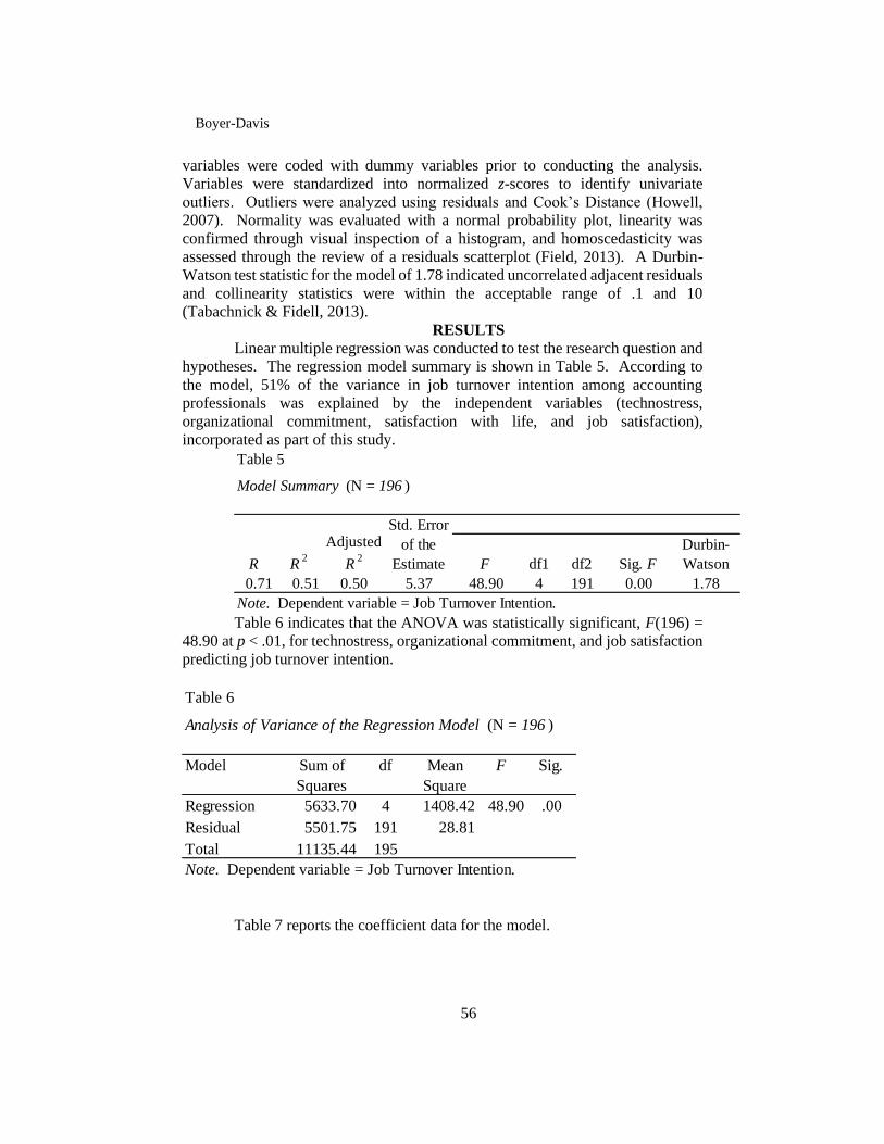
Boyer-Davis

56

variables were coded with dummy variables prior to conducting the analysis.

Variables were standardized into normalized z-scores to identify univariate

outliers. Outliers were analyzed using residuals and Cook’s Distance (Howell,

2007). Normality was evaluated with a normal probability plot, linearity was

confirmed through visual inspection of a histogram, and homoscedasticity was

assessed through the review of a residuals scatterplot (Field, 2013). A Durbin-

Watson test statistic for the model of 1.78 indicated uncorrelated adjacent residuals

and collinearity statistics were within the acceptable range of .1 and 10

(Tabachnick & Fidell, 2013).

RESULTS

Linear multiple regression was conducted to test the research question and

hypotheses. The regression model summary is shown in Table 5. According to

the model, 51% of the variance in job turnover intention among accounting

professionals was explained by the independent variables (technostress,

organizational commitment, satisfaction with life, and job satisfaction),

incorporated as part of this study.

Table 6 indicates that the ANOVA was statistically significant, F(196) =

48.90 at p < .01, for technostress, organizational commitment, and job satisfaction

predicting job turnover intention.

Table 7 reports the coefficient data for the model.

Table 5

Model Summary (N = 196 )

F df1 df2 Sig. F

Durbin-

Watson

0.71 0.51 0.50 5.37 48.90 4 191 0.00 1.78

Note. Dependent variable = Job Turnover Intention.

R R2

Adjusted

R2

Std. Error

of the

Estimate

Table 6

Analysis of Variance of the Regression Model (N = 196 )

Sum of

Squares

df Mean

Square

F Sig.

5633.70 4 1408.42 48.90 .00

5501.75 191 28.81

Total 11135.44 195

Model

Note. Dependent variable = Job Turnover Intention.

Regression

Residual


57

Technostress (β = .21, t(196) = p < .00), organizational commitment (β =

-.45, t(196) = p < .00), and job satisfaction (β = -.19, t(196) = p < .03), were

statistically significant in predicting job turnover intention in accounting

professionals. However, satisfaction with life was not significant (β = -.06, t(196)

= p < .28).

Table 8 summarizes the regression results and the overall findings of the

study based on the research question and sub-hypotheses.

DISCUSSION

This study identified that a relationship exists between

technostress and job turnover intention in the accounting profession. From a

practitioner standpoint, managers now have an awareness that technostress is of

considerable concern and can lead to an increased incident of job turnover rates in

the accounting profession. Firms are now able to strategize how to minimize the

stressors associated with technology.

One way that businesses can potentially curb technology stress is

to provide staff training prior to an implementation and system support thereafter.

Knowledge acquisition not only can reduce the uncertainty that employees feel

about the technology but can moderate the perception of its complexity. Likewise,

effective workplace communication is pivotal to lessen insecurities and

ambiguities surrounding a technology event. Companies should staff

appropriately so that role overload can be eased during the transition.

Table 7

Variables B SE β t Sig.

Constant 23.99 3.42 7.02 0.00

Technostress 0.06 0.02 0.21 3.79 0.00

Organizational Commitment -0.20 0.04 -0.45 -5.76 0.00

Satisfaction with Life -0.07 0.06 -0.06 -1.09 0.28

Job Satisfaction -0.04 0.02 -0.19 -2.17 0.03

Note. Constant (y-intercept). Overall model R2 = .71, F (4, 191) = 48.90, p = .001.

Multiple Regression Model Coefficient Data (N = 196 )

Table 8

Summary of Hypothesis Testing Results

Hypothesis Variable t Value Results

H1 Technostress .00 Rejected

H2 Organizational Commitment .00 Rejected

H3 Satisfaction with Life .28 Not Rejected

H4 Job Satisfaction .03 Rejected

Boyer-Davis

58

Employers should beware that policies that promote constant

connectivity by their employees may drive up technostress and cause job turnover.

Managers should respect employee personal time as much as possible and avoid

contact after hours. Furthermore, leaders should set the tone by unplugging

themselves.

In addition to the impact of job turnover, the economic blow of

technostress can be massive, equating to 225 million lost workdays and $300

billion in lost productivity per year (American Institute of Stress, 2007). Other

destructive outcomes include decreased profit and company value, a degradation

of services, and an increase in job vacancies (Moses, 2013). Technostress can

create a toxic work environment, accelerating workplace conflicts, permanently

damaging the corporate culture. This study has reinforced the merit of developing

approaches to lessen or eliminate the effects of technostress.

Companies should focus on improving the organizational commitment and

job satisfaction of their personnel since both were found to be negatively

associated with job turnover intention. Strategies such as building a culture of trust

and transparency, offering incentives, providing constructive criticism and

professional development opportunities, may be beneficial. Although the

satisfaction with life scale was not statistically significant in this study, work-life

balance has been identified as a highly critical component to retention rates.

Companies must continue to engage in work-life balance initiatives.

From a theoretical perspective, this landmark study established

that a statistical relationship exists between technology stress and job turnover in

the accounting profession. Future research should seek to determine causality

between technostress and job turnover using structural equation modeling. A

longitudinal study could be performed to measure the perceived variations in

technostress across the accounting profession. A final area of future research that

should be piloted is a cross-comparison of technostress among non-related

professions.

Limitations of the study include the use of a Likert-scale survey as a data

collection tool. Respondents were not provided with the opportunity to expand

upon or explain their answers. The study was limited to the accounting profession.

Results may differ in other occupations or industries. A survey panel was used to

gather data. Accountants not registered as part of the panel may have different

experiences than those surveyed for this study.

CONCLUSION

The accounting profession is poised for monumental change,

driven by advances in technology. Firms must carefully position themselves to

embrace the transformation without further driving up job turnover rates. Through

an awareness of and by implementing approaches to reduce technostress, the

accounting profession can be successful. The workforce will benefit from a more

technostress-conscious workplace.


59

REFERENCES

Agervold, M. (1987). New technology in the office: Attitudes and consequences.

Work & Stress, 1(2), 143-153.

Allen, N. J., & Meyer, J. P. (1996). Affective, continuance, and normative

commitment to the organization: An examination of construct validity.

Journal of Vocational Behavior, 49, 252-276.

American Institute of Stress. (2007). Job stress. Retrieved from

http://www.stress.org/job.htm

Asiedu-Appiah, F., Mehmood, A., & Bamfo, B. A. (2015). Work-life balance

practices, job performance and turnover intentions. International Journal

of Arts & Sciences, 8(4), 379-404.

Babbie, E. R. (2010). The practice of social research (12th ed.). Belmont, CA:

Wadsworth Cengage.

Bao, B., Bao, D., & Vasarhelyi, M. (1986). A stochastic model of professional

accountant turnover. Accounting, Organizations, and Society, 11, 289-

296.

Bedeian, A. G., & Armenakis, A. A. (1981). A path-analytic study of the

consequences of role conflict and role ambiguity. Academy of

Management Journal, 24, 417-424.

Benz, M., & Frey, B. S. (2008). Being independent raises happiness at work.

Swedish Economic Policy Review, 11, 95-134.

Boshoff, C., & Mels, G. (1994). A causal model to evaluate the relationships

among supervision, role stress, organizational commitment and internal

service quality. European Journal of Marketing, 29(2), 23-42.

Brillhart, P. E. (2004): Technostress in the workplace: Managing stress in the

electronic workplace. Journal of American Academy of Business,

Cambridge, 5, 302-307.

Brod, C. (1984). Technostress: The human cost of the computer revolution.

Boston, MA: Addison-Wesley.

Chen, G., Ployhart, R. E., Cooper Thomas, H., Anderson, N., & Bliese, P. D.

(2011). The power of momentum: A new model of dynamic relationships

between job satisfaction and turnover intentions. Academy of Management

Journal, 54, 159-181.

Chong, V. K., & Monroe, G. S. (2015). The impact of the antecedents and

consequences of job burnout on junior accountants’ turnover intentions: A

structural equation modelling approach. Accounting and Finance, 55, 105-

132.

Chua, S. L., Chen, D. T., & Wong, A. F. L. (1999). Computer anxiety and its

correlates: A meta-analysis. Computers in Human Behavior, 15(5), 609-

623.

Dale, K., & Fox, M. L. (2008). Leadership style and organizational commitment:

Mediating effect of role stress. Journal of Managerial Issues, 20(1), 109-

130.

Boyer-Davis

60

Diener, E., Emmons, R. A., Larsen, R. J., & Griffin, S. (1985). The Satisfaction

with Life Scale. Journal of Personality Assessment, 49(1), 71-75.

Doll, B. F. (1983). Staff turnover: How to manage it? Journal of Accountancy, 161,

76-82.

Drew, J. (2018). How AI, blockchain, and automation will reinvent accounting.

Journal of Accountancy. Retrieved from

https://www.journalofaccountancy.com/podcast/ai-blockchain-

automation-reinventing-accounting.html

Durndell, A., & Haag, Z. (2002). Computer self-efficacy, computer anxiety,

attitudes towards the Internet and reported experience with the Internet, by

gender, in an East European sample. Computers in Human Behavior, 18,

521-535.

Faul, F., Erdfelder, E., Lang, A. G., & Buchner, A. (2007). G*Power-3: A flexible

statistical power analysis program for the social, behavioral, and

biomedical sciences. Behavior Research Methods, 39(2), 175-191.

Felps, W., Mitchell, T. R., Heckman, D. R., Lee, T. W., Holtom, B. C., & Harman,

W. S. (2009). Turnover contagion: How coworkers’ job embeddedness

and job search behaviors influence quitting. Academy of Management

Journal, 52: 545-561.

Field, A. (2013). Discovering statistics using SPSS (3rd ed.). London, UK: Sage.

Fogarty, T. J., Singh, J., Rhoads, G. K., & Moore, R. K. (2000). Antecedents and

consequences of burnout in accounting: Beyond the role stress model.

Behavioral Research in Accounting, 12, 31-67.

Greenberg, J. (2005). Managing behavior in organizations, (4th ed). Upper Saddle

River, NJ: Pearson.

Greenhaus, J. H., Collins, K. M., & Shaw, J. D. (2003). The relation between work-

life balance and quality of life. Journal of Vocational Behavior, 63, 510-

531.

Gregson, T. (1992). An investigation of the causal ordering of job satisfaction and

organizational commitment in turnover models in accounting. Behavioral

Research in Accounting, 4, 80-95.

Grzywacz, J. G., Butler, A. B., & Almeida, D. (2009). Work, family, and health:

Work-family balance as a protective factor against stresses of daily life.

In The changing realities of work and family: A multidisciplinary

approach (pp. 194-215). Hoboken, NJ: Wiley-Blackwell.

Harrell, A. (1990). A longitudinal analysis of large CPA firm auditors’ personnel

turnover. Advances in Accounting, 8, 233-246.

Howell, D. C. (2007). The analysis of missing data. In W. Outhwaite, & S. Turner

(Eds.), Handbook of social science methodology (pp. 336-346). London,

UK: Sage.

Huselid, M. A. (1995). The impact of human resource management practices on

turnover, productivity, and corporate financial performance. Academy of

Management Journal, 30(4), 721-743.

https://www.journalofaccountancy.com/podcast/ai-blockchain-automation-reinventing-accounting.html

https://www.journalofaccountancy.com/podcast/ai-blockchain-automation-reinventing-accounting.html


61

Kahn, R. L., Wolfe, D. M., Quinn, R. P., Snock, J. D., & Rosenthal, R. A. (1964).

Organizational stress: Studies in role conflict and role ambiguity. New

York, NY: Wiley.

Kim, S. S., Im, J., & Hwang, J. (2015). The effects of mentoring on role stress, job

attitude, and turnover intention in the hotel industry. International Journal

of Hospitality Management, 48, 68-82.

Lambert, E. G., Hogan, N. L., Elechi, O. O., Jiang, S., Laux, J. M., Dupuy, P., &

Morris, A. (2009). A further examination of antecedents of correctional

staff life satisfaction. The Social Science Journal, 46, 689-706.

Lee, B. H., & Jamil, M. (2003). An empirical study of organizational commitment:

A multi-level approach. Journal of Behavioral and Applied Management,

4(3), 176-189.

Lee, S. H., & Jeong, D. Y. (2017). Job insecurity and turnover intention:

Organizational commitment as mediator. Social Behavior and

Personality: An International Journal, 45(4), 529-536.

Lee, S. H., Shin, Y., & Baek, S. I. (2017). Task characteristics and work

engagement: Exploring effects of role ambiguity and ICT presenteeism.

Sustainability, 9(10), 1-13.

Locke, E. A. (1976). The nature and causes of job satisfaction. In Handbook of

Industrial and Organizational Psychology. Chicago, IL: Rand McNally.

Linkedin. (2018). Linkedin data analysis reveals the latest turnover trends.

Retrieved from https://business.linkedin.com/talent-solutions/blog/trends-

and-research/2018/the-3-industries-with-the-highest-turnover-rates

Mathieu, J. E., & Zajac, D. M. (1990). A review and meta-analysis of the

antecedents, correlates, and consequences of organizational commitment.

Psychological Bulletin, 108(2), 171-194.

Mitra, A., Jenkins, G. D., & Gupta, N. (1992). A meta-analytic review of the

relationship between absence and turnover. Journal of Applied

Psychology, 77(6), 879-889.

Mitrovska, S., & Eftimov, L. (2016). Calculating the cost for employee turnover

in the IT industry in Macedonia by using a web calculator. Journal of

Human Resource Management, 19(1), 24-33.

Moses, O. S. (2013). Minimizing the effects of technostress in today’s

organization. International Journal of Emerging Technology and

Advanced Engineering, 3(11), 649-658.

Mowday, R. T., Porter, L. W., & Steers, R. M. (1979). The measurement of

organizational commitment. Journal of Vocational Behavior, 14, 224-247.

Nouri, H. (2017). Turnover in public accounting firms: The effect of position,

service line, ethnicity, and gender. Review of Business, 37(2), 14-27.

O’Reilly, C. (1989). Corporations, culture and commitment: Motivation and social

control in organizations. California Management Review, 31(4), 9-25.

Parker, R. J., & Kohlmeyer, J. M. (2005). Organizational justice and turnover in

public accounting firms: A research note. Accounting, Organizations and

Society, 30(4), 357-369.

https://business.linkedin.com/talent-solutions/blog/trends-and-research/2018/the-3-industries-with-the-highest-turnover-rates

https://business.linkedin.com/talent-solutions/blog/trends-and-research/2018/the-3-industries-with-the-highest-turnover-rates

Boyer-Davis

62

Pasewark, W. R., & Strawser, J. R. (1996). The determinants and outcomes

associated with job insecurity in a professional accounting environment.

Behavioral Research in Accounting, 8, 91-113.

Pew Research Center (2016). Public predictions for the future of workforce

automation. Retrieved from

http://www.pewinternet.org/2016/03/10/public-predictions-for-the-

future-of-workforce-automation/

Pitman, M. K., Gaertner, J. F., & Hemmeter, P. (2011). A study of male and female

employee turnover in public accounting firms. Journal of Applied

Business Research, 5(3), 10-15.

Pucci, E., Cristina, S., Antonaci, F., Costa, A., Imbriani, M., & Taino, G. (2015).

Technostress and primary headache: Psychosocial risk. The Journal of

Headache and Pain, 16(1), 29-31.

Riedl, R., Kindermann, H., Auinger, A., & Javor, A. (2012). Technostress from a

neurobiological perspective: Systems breakdown increases the stress

hormone cortisol in computer users. Business & Information Systems

Engineering, 4(2), 61-69.

Schieman, S., Milkie, M. A., & Glavin, P. (2009). When work interferes with life:

Work-nonwork interference and the influence of work-related demands

and resources. American Sociological Review, 74(6), 966-988.

Senatra, P. T. (1980). Role conflict, role ambiguity, and organizational climate in

a public accounting firm. The Accounting Review, 55, 594-603.

SHRM, (2014). Turnover cost calculator. Retrieved from

https://www.shrm.org/resourcesandtools/tools-and-samples/hr-

forms/pages/1cms_011163.aspx

Siu, O. L. (2003). Job stress and job performance among employees in Hong Kong:

The role of Chinese work values and organizational commitment.

International Journal of Psychology, 38(6), 337-347.

Spector, P. E. (1985). Measurement of human service staff satisfaction:

Development of the Job Satisfaction Survey. American Journal of

Community Psychology, 13(6), 693-713.

Tabachnick, B. G.. & Fidell, L. S. (2013). Using multivariate statistics (6th ed.).

New York, NY: Pearson Education, Inc.

Tarafdar, M., Tu, Q., Ragu-Nathan, B., & Ragu-Nathan, T. (2007). The impact of

technostress on role stress and productivity. Journal of Management

Information Systems, 24(1), 301-328.doi:10.2753/MIS0742-1222240109

Tarafdar, M., Tu., Q., Ragu-Nathan, T. S., & Ragu-Nathan, B. S. (2011). Crossing

to the dark side: Examining creators, outcomes, and inhibitors of

technostress. Communications of the ACM, 54(9), 113-120.

Tett, R. P., & Meyer, J. P. (1993). Job satisfaction, organizational commitment,

turnover intention and turnover: Path analyses based on meta-analytic

findings. Personnel Psychology, 46(2), 259-293.

Toker, B. (2012). Life satisfaction among academicians: An empirical study on the

Universities of Turkey. Social and Behavioral Sciences, 47, 190-195.

https://www.shrm.org/resourcesandtools/tools-and-samples/hr-forms/pages/1cms_011163.aspx

https://www.shrm.org/resourcesandtools/tools-and-samples/hr-forms/pages/1cms_011163.aspx

http://dx.doi.org/10.2753/mis0742-1222240109


63

Tu, Q., Ragu-Nathan, B., & Ragu-Nathan, T. S. (2001). A path analytic study of

the antecedents of organizational commitment of IS managers.

Information Resources Management Journal, 14(3), 27-36.

U.S. Bureau of Labor Statistics. (2018). Job openings and labor turnover,

September 2018 report. Retrieved from https://www.bls.gov/jlt/

Vakola, M., & Nikolaou, I. (2005). Attitudes towards organizational change: What

is the role of employees’ stress and commitment? Employee Relations,

27(2), 160-174.

Viator, R. E. (2001). The association of formal and informal public accounting

mentoring with role stress and related job outcomes. Accounting,

Organizations and Society, 26, 73-93.

Walsh, J. P., Ashford, S. J., & Hill, T. E. (1985). Feedback obstruction: The

influence of the information environment on employee turnover. Human

Relations, 38(1), 23-46.

Wright, K. B., Abendschein, B., Wombacher, K., O’Connor, M., Hoffman, M.,

Dempsey, M., Krull, C., Dewes, A., & Shelton, A. (2014). Work-related

communication technology use outside of regular work hours and work

life conflict: The influence of communication technologies on perceived

work life conflict, burnout, job satisfaction, and turnover intentions.

Management Communication Quarterly, 28(4), 507-530.

https://www.bls.gov/jlt/



64

THE COMPREHENSIVE TAXATION SYSTEM

EXISTING DURING THE ROMAN EMPIRE

Darwin L. King

Carl J. Case

Jared L. Roosa

St. Bonaventure University

ABSTRACT

This paper reviews the various forms of Roman taxes that existed during

the period of the Roman Empire. The first section of this paper reviews the

tremendous growth of the Roman Empire over several hundred years. In order to

fund the expansion of the empire and fund the armies, Roman rulers utilized a wide

variety of taxes. The intent of this paper is to review the extremely large amount

of taxes that were extracted from inhabitants of Roman conquered lands. Roman

taxes were in addition to religious taxes paid by Jewish inhabitants of all Roman

controlled lands. This created a system of double taxation which became very

oppressive to those affected.

The first portion of this paper briefly traces the growth of the Roman

Empire over the period from 753BC to 476AD. The major portion of this paper,

however, reviews the Roman taxation system in existence during the years that the

empire existed. Following the brief summary of the growth of the Roman Empire,

but prior to an analysis of the Roman taxation system, is a discussion of the

occupation of the “tax collector” or “publican.” The occupation of tax collector or

“tax farmer,” during this period, was one of very low social status equal to that of

prostitutes and other unsavory vocations. The final portion of this paper reviews

the question of whether or not the inability to assess and collect these various taxes

may have contributed to the fall of the Roman Empire.

Key words: Roman empire, comprehensive taxation system, Romulus and

Remus, Julius Caesar

INTRODUCTION

One of the most impressive civilizations in history is that of the Romans.

Most historians trace the Roman Empire over a period of many centuries.

Depending of the historian, the Roman Empire began with the founding of Rome

by the twin brothers Romulus and Remus (Sidebottom, 2016). As legend has it,

Romulus founded the city on the Palatine Hill. This paper focuses on the taxes that

the Roman government employed to fund all its expenditures including those


65

needed to support the armies. Similar to the taxation system of today, taxes took

many forms including an income tax, a sales tax, various property taxes, and

numerous customs fees and duties.

This paper begins with an overview of the growth and expansion of the

Roman Empire from approximately 753 BC (or BCE) to 476 AD (or CE). The

authors will use the traditional BC (Before Christ) and AD (Anno Domini - Latin

for year of the Lord) in this paper instead of the BCE (Before the Common Era)

and CE (Common Era) designations. Depending on the historian, the period of the

Roman Empire may differ significantly from the dates mentioned above. However,

the authors will adhere to these dates mentioned above. The following paragraphs

discuss the growth of the Roman Empire.

ORIGIN AND GROWTH OF THE ROMAN EMPIRE

During very early times, many Roman citizens believed that Rome was

founded precisely in 753 BC (Sidebottom, 2016). This is the date of the traditional

story when the twins, Romulus and Remus, sons of the god Mars, were placed in

a basket on the river Tiber and left to die. The basket landed on the riverbank at

the future location of the city of Rome. The babies were nursed by a female wolf

and later raised by a local shepherd.

Sidebottom continues the Romulus/Remus myth that disclosed that upon

adulthood Romulus founded the city of Rome on Palatine Hill and killed his

brother Remus. The story is very similar to the Bible’s Old Testament story of Cain

and Able where brother also killed brother. Although Sidebottom admits that there

is no basis in fact for the Romulus and Remus story, he states that archeologists

have found evidence of a city on Palatine Hill as early as 1,000 BC (Sidebottom,

2016). Although an exact date cannot be accurately determined when the city of

Rome first appeared, historian agree that it was at approximately this date.

N.S. Gill provides a brief summary of the periods of history in ancient

Rome (Gill, 2017). He identifies these periods as Regal Rome, Republican Rome,

the Roman Empire, and the Byzantine Empire. The following paragraphs briefly

summarize each of these periods which begin in 753 BC and conclude in 476 AD

(or as late as 1453 AD according to some historians).

Gill states that the Regal Period lasted from 753 BC to 509 BC. This was

a period when kings ruled over Rome with the first being Romulus. Romulus,

according to legend, was the son of the god Mars and a Vestal Virgin named Rhea

Silvia (Gill, 2017). Gill believes that the brothers, Romulus and Remus, were

raised by a prostitute rather than a she-wolf, since the Latin word for brothel is

“lupanar.” The Latin for both prostitute and she-wolf is “lupa.”

Gill also describes a second version of the founding of Rome. The Roman

poet Virgil describes, in the Aeneid, the founding of the town of Lavinium by

King, Case and Roosa

66

Aeneas in approximately 1176 BC. Ascanius, son of Aeneas, built the city of Alba

Longa in 1152 BC. Both these cities were located where the future city of Rome

would be built.

Gill adds that most of what is known about early Rome comes from the

Roman historian, Titus Livius (or Livi) (Livius, 1928). He lived from 59 BC to 17

AD and authored the text “History of Rome From Its Foundation.” Both six and

two volume sets of this work are available online (public domain).

As mentioned above, during the Regal period of 753 BC to 509 BC, Rome

was ruled by seven Kings. Gill adds that legend has it that the Seven Hills of Rome

are associated with these seven original kings. Romulus was king from 753-715

BC. He was followed by Numa Pompilius (715-673 BC), Tullus Hostilius (673-

642 BC), Ancus Martius (642-617 BC), L. Tarquinius Priscus (616-579 BC),

Servius Tullius (578-535 BC), and finally Tarquinius Superbus (Tarquin the

Proud) (534-510 BC). Legend has it that Superbus came into power following the

assassination of Servius Tullius. Superbus and his family were purported to be so

evil and vicious that legend states they were forcibly removed from power by

Brutus and other members of the Senate (Gill, 2017). During this period, the kings

answered to the Senate and did not possess absolute power.

Gill identifies the second period in Roman history as the Roman Republic

or Republican Rome which lasted from 509 BC to 27 BC (Gill, 2017). During this

period, Rome elected the governor of the various regions. To prevent abuse of

power, the Romans allowed the “comitia centuriata” to elect a pair of top officials

who were called “consuls.” The comitia centuriata was a political assembly

comprised of 30 kinship groups into which Roman families were divided. These

kinship groups (called curiae) were comprised of three families that existed when

Romulus was king. These tribes were the Ramnenses, Titienses, and Luceres (Gill,

2017).

The consuls were elected Roman magistrates during the Roman

Republican Period (Gill, 2018). By 181 BC, these men had to be at least 43 years

old and of good character. These individuals possessed a limited term of near

absolute power. They were, however, less powerful than the king because their

term was limited to one year and the power was split between the two consuls.

Consuls were very powerful, since they were responsible for decisions on war,

justice, and finance. Each consul had the power to negate the other. They were,

however, supposed to abide by the senate’s advice.

One of the most important figures during the Roman Republic period was

Julius Caesar who was born in 100BC and lived until he was assassinated on March

15, 44 BC by Marcus Brutus. According to History.com authors, the assassination

conspiracy may have included as many as 60 of his senators who were angry about

the prospect of taking orders from Caesar’s subordinates. These individuals were


67

scheduled to replace Caesar while he was off fighting a war scheduled to begin on

March 18th (History.com authors, 2009).

The third period of the history of Rome, the Roman Empire or Imperial

Rome, according to historiography convention, dates from 27 BC to 284 AD

(Encyclopedia Britannica, 2018). During the period, the Roman Empire spread at

an astounding rate. According to Joshua Mark, the Roman Empire, at its height in

117 AD was the most extensive political and social structure in western civilization

(Mark, 2018). The Roman Empire was so vast in 285 AD that Emperor Diocletian

divided it into a Western and Eastern Empire. The Eastern Empire remained strong

(after 476 AD) operating out of its capital city of Constantinople created by

Emperor Constantine in 330 AD.

This “two headed” empire (Rome and Constantinople) was firmly

established by 395 AD. During this period, Rome was extremely powerful

controlling the Mediterranean, the Balkans, Turkey, and the modern areas of the

Netherlands, southern Germany, France, Switzerland, and England (Gill, 2017).

The Western Empire was dissolved in 476 AD when Rome fell to Germanic King

Odoacer. Some authors consider this date to be the close of the Roman Empire

while others consider the end of the empire to be nearly 1,000 years later.

The fourth period of the history of Rome centered upon the Eastern Empire

referred to as the Byzantine Empire (Mark, 2018). As mentioned above, the capital

city was Constantinople which is modern-day Istanbul. When King Odoacer seized

Rome in 476 AD, he did not destroy the Roman Empire in the east which is known

today as the Byzantine Empire (Gill, 2017). Residents of this area spoke either

Greek or Latin but were citizens of the Roman Empire. However, the culture in

this area was more Greek than Roman.

Although the Western Empire collapsed in 476 AD, the Eastern Empire

continued to exist for approximately 1,000 years. It was not until the Ottoman

Turks conquered the area in 1453 AD (Gill, 2017) Using this date, most historians

identify the timeline for the Roman Empire to begin in 753 BC and end in 1453

AD. This 2,200 year period marked the beginning and end of one of the most

recognized and respected civilizations in our history.

The remainder of this paper will review several types of taxes assessed

upon residents of the Roman Empire. A comprehensive tax system was essential

in order to finance the cost of the Roman armies and provide services for all

inhabitants of the vast empire. Prior to the review of the Roman tax system, a

description of the duties and responsibilities of a publican or tax farmer (collector)

is appropriate.


68

THE PROFESSION OF PUBLICAN OR TAX COLLECTOR (FARMER)

The word “publican” is an English translation of the Greek word “telones”

which means “tax-farmer” (Badian, 1983). Therefore, a publican had the task of

collecting taxes for the Roman government. During the period of the expansion of

the Roman Empire, these individuals would bid to acquire a “tax franchise” for a

particular area that enabled them to collect a variety of taxes from occupants of the

area. These tax farmers were responsible for converting taxes collected in-kind

(crops/animals) into hard currency. Therefore, publicans collected enough money

from taxpayers to cover the taxes due, exchange fees, and provide themselves with

a profit. (Bartlett, 1994). In addition to an already extravagant salary, the publicans

would collect additional taxes above those required by Rome which would further

increase their total income.

During the first century AD, Jerusalem was under Roman control being

conquered by Roman general Pompey during his eastern campaign when he

established the Roman province of Syria in 64 BC and conquered the city of

Jerusalem in 63 BC (Barraclough, 1981). In this region, publicans were typically

Jews who worked for the despised Roman government collecting various taxes

from Jewish citizens. Publicans were despised in most cultures, since they were

automatically assumed to be dishonest, unethical, and without character.

Basically, the invading Roman government employed citizens of

conquered lands to perform the undesirable task of collecting taxes. The Roman

government accomplished this by promising significant bonuses. This allowed the

publicans to extort as much money as possible from the local citizens thereby

increasing the publican’s total income. It is easy to imagine the significant

corruption that existed in this type of tax collection system. It is also

understandable that the publicans were despised and deemed to be traitors to their

own nation. Given this situation, publicans had few friends and were forced to

associate with other publicans or the criminal element of the population. The Bible

states, in many of its books, that association with a publican automatically cast

suspicion on that person’s reputation.

The Bible reports that Jesus was often found in the company of publicans.

For example, one of the disciples, Matthew (also called Levi) was a tax collector.

“And as Jesus passed forth from thence, he saw a man, named Matthew, sitting at

the receipt of custom: and he saith unto him, Follow me. And he arose, and

followed him” (Matthew 9:9). This appalled the religious Jewish leaders as verse

11 continues with, “And when the Pharisees saw it, they said unto his disciples,

Why eateth your Master with publicans and sinners?” The Bible contains many

verses where tax collectors are on the same level as prostitutes and other

undesirables such as Matthew 21:32 (publicans and prostitutes (harlots)), Luke

5:30 (publicans and sinners), and Mark 2:16 (publicans and sinners).


69

John MacArthur also comments on the social status of the publican. He

discusses the disciple Matthew who possessed the occupation least likely to

warrant discipleship. MacArthur states that tax collectors were the most despised

people in Israel (MacArthur, 2002). He states the citizens of that period deemed

them to be lower and more worthy of scorn that the occupying Roman Army.

MacArthur reports that publicans extorted money from the people often using hired

thugs. In his words, publicans were considered “despicable, vile, unprincipled

scoundrels.” MacArthur states that publicans had an unspoken agreement with the

Roman Emperor that besides collecting legitimate taxes owed to Rome that they

could also assess additional fees and taxes. These additional monies could be

retained by the publican in full or shared with Rome on a percentage basis.

MacArthur reports that there were two types of tax collectors known as

the “Gabbai” and the “Mokhes” (MacArthur, 2002). The first group (Gabbai) were

general tax collectors who collected property, income, and poll taxes. The second

type (Mokhes) collected duties on imports and exports, goods for domestic trade,

and virtually everything that was moved by road. In addition, they established tolls

on roads and bridges, taxes on beasts of burden, and taxes on transport wagons

based on the number of axles. Finally, MacArthur added that publicans were

allowed to assess taxes on packages/parcels, letters, and any other type of personal

property.

There were two types of Mokhes referred to as the Great Mokhes and the

Little Mokhes (McArthur, 2002). A Great Mokhes operated behind the scenes and

hired others to actually collect the taxes in his place. A Little Mokhes operated a

tax office where he would deal with people on a face to face basis. MacArthur

believes that the disciple Matthew was a Little Mokhes because he was dealing

with people face-to-face at a tax office when Jesus found him (Matthew 9:9).

MacArthur stresses how much publicans were hated by the local people. He states

that no self-respecting Jew would become a tax collector. This action cut him off

from his people and his God, since he was banned from the synagogue and

forbidden to sacrifice and worship in the temple. As mentioned earlier, the

publicans had few friends other than fellow publicans and the socially undesirable.

George Shillington discusses the “Tale of Two Taxations” (Shillington,

1997). This relates to taxation at the time of Christ during the first century AD.

Inhabitants of Jerusalem during this period were required to pay both Roman and

Jewish taxes which created a dual tax system. The publicans were especially hated

because they extracted money from Jewish residents that was budgeted for one of

their three required religious taxes. These included a wave or first fruits offering

of typically 3%, a 10% annual tithe (for support of the priests and Levites), and a

second 10% tithe for a total of approximately 23%. The second portion of the dual

tax system included the Roman taxes collected by the publicans. Shillington

references Titus Flavius Josephus who wrote that the primary taxes extracted by

the Romans were the poll (head tax) and land taxes. In addition to these two taxes,


70

the Roman government also collected various land transfer taxes, export and

import duties, and a real estate tax on all the houses in Jerusalem (Josephus,

78AD). It is easy to understand the hatred towards the Publicans who extracted

numerous taxes to finance a foreign government. This left residents of conquered

lands with less funds to pay necessary living expenses and pay required Jewish

religious taxes identified in both the books of the old and new testaments of the

Bible.

The next portion of this paper identifies the significant number of taxes

that were utilized by the Roman government. These included real estate taxes,

excise and custom taxes, marriage taxes on unmarried men and women who could

not bear children, inheritance taxes, poll taxes, and many more. The final segment

of this paper reviews the question of whether massive tax evasion was a major

reason for the fall of the Roman Empire.

THE EXTENSIVE ROMAN TAXATION SYSTEM

The Roman Empire extracted a number of direct and indirect taxes or

tributes. The two basic types of direct taxes were tributum soli and tributum capitis

(Encyclopedia Britannica, 2018). According to Brunt, tributum soli was a tax on

the land (Brunt, 1981). It was not a tax on harvests or crops. Nor was it a tax on

“movables” such as slaves, animals, and equipment for cultivating and processing

crops. Since land was the chief source of wealth during the period of the Roman

Empire, the land tax produced the majority of total tax revenues.

Caesar Augustus (or Octavian until 27BC), the first Roman emperor,

following the republic, from 30BC to 14AD, established a number of fiscal and

monetary reforms. In particular, he introduced three new taxes including a land tax

(tributum soli), a general sales tax, and a flat-rate poll tax (tributum capitis)

(Davies, 2002). The tributum soli or land tax was established at one percent of the

assessed value of the land. The general sales tax of 1% and flat-rate poll tax on

adults from the age of 12 or 14 to age 65 will be discussed later in this paper.

Brunt states that in the Roman census process, the imperial government

had a model for registration and taxation of all forms of property including both

real and tangible personal property. This included land, buildings, cash, debts due

from others (accounts receivable), clothing, jewels, and slaves (Brunt, 1981). The

worth of all these forms of capital was valued apparently using a set of formulas

established by the censors who were government officials who conducted the

census. This valuation system required the possessors of the land to specify the

acreage that could be cultivated and farmed, the number of grade vines, and the

acreage containing olive trees (Brunt, 1981).

Since the land tax was such a vital part of the Roman taxation system, there

were significant penalties for false declarations concerning the acreage and value

of the property. Slaves implicated in the frauds would often suffer death. The


71

testimony of slaves was often sufficient to convict the land owner. Septimius

Severus, Roman emperor from April 193AD to February 211AD ruled that slaves

could be examined against their owners for only the crimes of census fraud and

adultery (Brunt, 1981).

A second type of Roman tax was called “Collatio lustralis” or a tax on

“traders in the widest sense.” It was a tax on anyone who produces a product or

provides a service, with the exception of farmers, physicians, and teachers (Oxford

Classical Dictionary, 1970). This tax was instituted by Constantine, Roman

Emperor who ruled from 306 to 337AD. According to the Byzantine writer

Zosimus, Constantine established this tax as early as 325AD (Goffart, 1971).

The tax was originally collected annually in either gold or silver but in the

late 4th century it was only payable in gold. In the early 5th century, the tax was

required to be paid once every four years. Zosimus reported the extreme hardship

caused by this tax, since it was collected in a lump sum every four years (Goffart,

1971). It was devastating to parents who were forced into selling their children into

slavery or prostitution in order to pay this tax.

The tax was abolished by Anastasius I in 498AD in the Eastern Roman

Empire as part of his monetary and fiscal reforms (Nicks, 1998). Anastasius was

known for his administrative efficiency. For example, he changed the payment

method for governmental transactions from goods to hard currency (Treadgold,

2001). Upon leaving the imperial government, he was recognized for establishing

a significant budget surplus due to internal controls introduced to minimize

governmental corruption. The state treasury, at the time of his death, was three

hundred and twenty thousand pounds (Nicks, 1998). In addition, Anastasius

reformed the tax code of the period and introduced an improved form of currency

(Treadgold, 2001).

A third type of Roman tax was called Portoria which was also referred to

as a harbor or customs tax. This was a 2½% ad valorem (based upon value) tax

collected in virtually every port in the Mediterranean on nearly every type of

product (Finley, 1973). The only items exempted from the tax were shipments of

imperial annona (corn supplies) for the armies and the citizens of Rome.

The system supplying Rome, the armies, and other valuable cities with

grains (mainly corn) and other foodstuffs came to be known as the annona

(Erdkamp, 2016). The grain distribution system was first introduced in 123BC by

C. Sempronius Gracchus (a Roman populist and reformist politician). Given that

the harbor tax or customs duty was assessed on virtually all goods moving in and

out of Mediterranean ports, this tax produced significant revenue for the Roman

government. This system ended in 429AD when Africa was conquered by the

Vandals, since most grains at this time were shipped to Rome from African ports.

https://en.wikipedia.org/wiki/Ancient_Rome

https://en.wikipedia.org/wiki/Populares


72

The Roman tax system also included two taxes assessed on orphans,

widows, and single women that was used for the purchase and upkeep of the

Roman army’s horses. These taxes were termed “aes equestre” and “aes

hordearium” (Hill, 1943). The aes equestre was the monetary sum of 10,000 asses.

The as (plural asses) was originally introduced in approximately 280BC as a large

cast bronze coin (later copper) that was minted during the periods of the Roman

Republic and Roman Empire.

The aes equestre was given to a cavalry soldier often called the “equus

publicus” (equestrian order) for the purchase of a horse. The equus publicus was a

wealthy secondary property-based class of ancient Rome who ranked below the

senatorial class. In more modern times, this class would have been known as

“knights.” Therefore, the cavalry was composed of men from fairly affluent

heritage.

The aes equestre was collected from single women (maidens and widows)

and orphans provided that they owned a certain amount of property (Smith, 1875).

This was based on the argument that women and children should contribute to the

military who fight on their behalf. The Roman government deemed this to be a fair

tax given the fact that women and children were not included in the census and

therefore were exempt from other taxes such as the poll tax which was assessed

primarily on adult men (Niebuhr, 1835). Revenue from this tax was deposited and

accumulated in the public treasury. Later, these revenues were paid from the public

treasury to a cavalry soldier in lots of 10,000 asses in order to purchase a horse

(Smith, 1875).

The aes hordearium amounted to the sum of 2,000 asses annually for the

care and feeding of a horse (Smith, 1875). Like the aes equestre, the tax was

assessed against single women and orphans who owned a certain amount of

property. In other words, it was not collected from women and orphans who had

little or no assets. The cavalry soldier received this annual 2,000 asses stipend from

the public treasury at the rate of 200 asses per month for 10 months (Niebuhr,

1835).

Niebuhr states that in these early times ten months were considered to be

one year and 10 months times the 200 asses per month equals the aes hordearium

total of 2,000 asses for a year. He continues that the cavalry rate of 200 asses per

month was twice the 100 asses received by a foot-soldier or infantryman (Niebuhr,

1835). Niebuhr adds that generals in the Roman Army received 300 asses per

month. The general’s triple pay (triple the infantryman’s salary of 100 asses) was

introduced in 354AD by the military tribune Cn. Cornelius Cossus (Niebuhr,

1835).

Another Roman tax was called the “aes uxorium” which was a tax imposed

upon women who could not bear children, with the exception of Vestal Virgins,


73

and unmarried men who had reached adulthood without marrying (Peck, 1898). It

was first introduced by the censors M. Furius Camillus and M. Postumius in

403BC (Smith, 1875). This tax did not apply to unmarried men age 60 and older

nor to unmarried women age 50 or more. It is uncertain how long this tax remained

in existence.

Prior to the reign of Rome’s first emperor, Augustus Caesar, from 27BC

to 14AD, no inheritance taxes were recorded for the Roman Republic. Augustus

introduced the “vicesima hereditatium” or inheritance tax of approximately 5%

(Gardner, 2001). This tax applied to inheritances that were received by way of a

will and any close relatives were exempt from paying it. Close relatives included

the deceased individual’s grandparents, parents, children, grandchildren, and

siblings. Roman custom from the late Roman Republic and afterwards was that

husbands and wives kept their own property separate from that of the spouse. This

resulted in Roman women remaining a part of her birth family. She was not

considered to be under the legal control of her husband. Therefore, in many cases

it was questionable if the wife was exempt from the tax. Many authors feel that

Roman social values regarding marital devotion probably exempted the wife from

tax in most cases (Gardner, 2001).

Another tax that was introduced by Augustus Caesar was a 1% general

sales tax (Davies, 2002). The tax was designed to fund the military and was

instituted in approximately 6AD. It was termed the “centesima rerum venalium”

which roughly translates to “a hundredth of the value of everything sold.” This tax

was later reduced to one half percent by Tiberius and finally eliminated by

Caligula. Tiberius was emperor from 14AD to 37AD following Augustus. Caligula

followed Tiberius as emperor from 37AD to 41AD. This unpopular sales tax

existed for less than 40 years.

A Roman tax that was specifically imposed upon Jewish people living in

the Roman Empire was called the “fiscus Judaicus” (Gottheil & Krauss, 1906).

According to Josephus, the tax was imposed by Roman Emperor Vespasian as a

result of the First Roman-Jewish War (first Jewish revolt) of 66-73AD. The tax

was imposed following the destruction of the second Temple in 70AD. This two

denarii (or one-half shekel) tax was in place of the Temple tax (Exodus 30:vs.11-

13) paid in prior years by the Jewish people for the upkeep of the Temple. This tax

was a major humiliation for the Jews who had just experienced the destruction of

their Temple for the second time. Unlike the Temple tax of previous years that was

paid only by adult men between the ages of 20 and 50, the fiscus Judaicus was

imposed on all Jewish people including women, children and the elderly (Schäfer,

1998).

The extensive Roman tax system also included a poll or head tax (of two

denarii) called the “tributum capitis” (Digest 50, tit.15, 1932). The Roman

government imposed this direct tax on all the people living in the controlled


74

provinces. This tax was assessed primarily on the Roman subjects living in the

provinces and not on Roman citizens. For this reason, it was a much hated tax

referred to by Tertullian (an early Christian author) as a "badge of slavery." (Audi,

(1999). According to Tertullian, this tax provoked numerous civil revolts. The

most famous of these being the Zealot revolt in Judea in 66AD following the

destruction of the temple in 70AD. These taxes were typically collected by the

private tax farmers or publicans discussed earlier. According to Tertullian, these

taxes were assessed annually on males over age 14 and females over age 12 until

they reached the age of 65.

The final two Roman taxes included in this paper are typically called slave

taxes (Bradley, 2016). The “vicesima libertatis” was a tax on slave owners who

freed slaves. The tax was 5% of the value of the slave (Dilke, 2016). The tax was

either paid by the owner, if he freed the slave, or by the slave, if he redeemed

himself with his own money. The second slave related tax was called the “quinta

et vicesima venalium mancipiorum.” This was a 4% tax on the owners who sold

slaves (Dilke, 2016). Information is very scarce concerning these taxes such as the

years they existed and the methods used to value the slaves. No doubt age and sex

were important assessment factors but details on this valuation process have been

lost over the centuries.

It is obvious that the Romans were forced to utilize a wide range of taxes

in order to finance the expansion of the empire and purchase food, supplies, and

armaments for the armies. In addition, funds were needed to purchase food for the

large population (approximately one million) living in the city of Rome. Davies

estimates that Rome needed to import at least 150,000 tons of grain each year to

feed the inhabitants (Davies, 2002). Much of this grain was needed to feed the poor

of the city. Davies states that as many as 200,000 of the poor in Rome received

free distributions of wheat from the Roman government. It is not surprising that

the cost of funding the armies and expanding the empire required the emperors to

consider all possible forms of additional tax revenues.

A number of Roman emperors revised and modified the monetary and tax

system for Rome. One of the most successful in these endeavors was Augustus

Caesar emperor from 30BC to 14AD. He instituted a set of three principal taxes to

generate the much needed revenues for the period (Davies, 2002). As mentioned

earlier, these included a 1% sales tax, a 1% tax on land (tributum soli), and the poll

or head tax of two denarii on men aged 14 to 65 and women aged 12 to 65. Many

of details of the taxes discussed above have be lost over the centuries such as the

exact year introduced and removed. Finally, an interesting fact is that the majority

of the Roman taxes (real estate, sales, etc.) discussed in this paper are still common

today in many countries around the world.


75

FINAL THOUGHTS – TAXES AND THE DECLINE OF THE ROMAN

EMPIRE

No doubt the decline of the Roman Empire was the result of numerous

factors. However, two of the major causes for the decline could have logically been

the widespread tendency of the people to evade as many of the multitude of taxes

as possible and the inefficient and ineffective tax assessment and tax collection

processes of the Roman government.

Pulliam discusses a number of reasons why significantly more taxes were

collect than were actually deposited with the Roman government (Pulliam, 1924).

In addition to taxpayers evading these taxes, there was also a huge amount of fraud

and embezzlement on the part of tax assessment and tax collection personnel.

Pulliam argues that that “while the revenue secured was usually adequate for all

expenses of the government, the system of taxation had a number of serious defects

(Pulliam, 1924).

The primary defect, according to Pulliam, was the method of collecting

the taxes. As discussed earlier in this paper, the publicans (tax farmers) were

considered cheats and fraudsters. Pulliam states that publicans collected exorbitant

amounts of tax well above the required amount. He says that the publican became

the “most odious figure in provincial life and perhaps the most galling feature of

Roman domination was the tax that Rome collected” (Pulliam, p.548).

The second basic problem of the Roman tax system, according to Pulliam

was the range of duty rates charged on goods moved from one province to another.

The trade districts were often arbitrarily determined and did not correspond to

provincial boundaries (Pulliam, p.548). Pulliam states that the duties on goods

going from one province to another were much higher than goods going from a

province to Rome. In addition, harbor duties and road and bridge tolls made the

cost of transporting products from province to province cost prohibitive. Pulliam

argues that free movement of trade throughout the empire would have increased

the overall wealth of the empire significantly.

A final problem of the Roman Empire taxation system, according to

Pulliam, was the lack of overall general administration (Pulliam, p.549). The

Roman government never attempted to appoint an experienced, effective, and

efficient manager to the finance and taxation department of the government. The

head of finance and expenditures, called a “quaestor,” served for only one year

thereby never becoming familiar with the details of the financial management area

of the government. Pulliam states that the budgeting process was nonexistent and

that there was no attempt to balance taxation revenues and government

expenditures.


76

SUMMARY AND CONCLUSIONS

This paper reviewed many of the taxes collected by the Roman

government during the period of the Roman Empire. It appears that most every

type of tax in existence today is rooted in the history of the Roman Empire which

covered many centuries from 753BC to 476AD. The tax system of this period was

a major hardship on the people living within the empire. This resulted, in large

part, from the fraudulent and dishonest actions of the publicans or tax collectors of

the period. It is easy to understand the importance of internal controls in today’s

business environment. Unfortunately, such controls did not exist during the period

of the Roman Empire.

REFERENCES

Audi, R. (1999). The Cambridge Dictionary of Philosophy. Cambridge

University Press, 908.

Badian, E. (1983). Publicans and Sinners. Cornell University Press

Barraclough, G., ed. (1981). The Times Atlas of World History.

Bartlett, B. (1994). How Excessive Government Killed Ancient Rome, Cato

Journal, 14. 2 (Fall).

Bradley, K. (2016). The vicesima libertatis: Its History and Significance. Klio,

66.66, 75-182. Retrieved, from doi:10.1524/klio.1984.66.66.175.

Brunt, P. (1981). The Revenues of Rome. The Journal of Roman Studies, 71,

161-172. doi:10.2307/299505

Davies, G. (2002). A History of Money, University of Wales Press,

Cardiff, 96. Digest 50, tit.15, 1932.

Dilke, O. A. W. (1987). Mathematics and Measurement, Berkeley:

University of California Press, 51.

ENCYCLOPEDIA BRITANNICA. (2018). ROMAN EMPIRE ANCIENT

STATE [27 bc-476 ad], retrieved from

https://www.britannica.com/place/roman-empire

Erdkamp, P. (2016). Annona (grain), Oxford Classical Dictionary. Retrieved

from http://oxfordre.com/classics/view/10.1093/acrefore/

Finley, M. I. (1973). The Ancient Economy, University of California Press,

Berkeley and Los Angeles, CA.,159.

https://en.wikipedia.org/wiki/Geoffrey_Barraclough

https://en.wikipedia.org/wiki/The_Times_Atlas_of_World_History

https://www.britannica.com/place/roman-empire


77

Gardner, J. F. (2001). Nearest and dearest: liability to inheritance tax in Roman

Families, Class and Kin in the Roman World. Routledge, 205-220.

Gill, N.S. (2107). Periods of History in Ancient Rome, Thought Co.

Retrieved from https://www.thoughtco./periods-of-ancient-rome.

Gill, N.S. (2107). Romulus-Roman Mythology About the Founding and First

King of Rome, Thought Co. Retrieved from

https://www.thoughtco.com/romulus-roman-mythology.

Gill, N.S. (2107). Who Were the Early Kings of Rome? Thought Co.

Retrieved from https://www.thoughtco.com/the-early-kings-of-rome

Gill, N.S. (2108). Who Were the Roman Consuls and How Did They Rule

Rome? Thought Co. Retrieved from https://www.thoughtco.com/who-

were-the-roman-consuls

Goffart, W. (1971). Zosimus, The First Historian of Rome's Fall. The

American Historical Review, 76.2, 412-441. doi:10.2307/1858706

Gottheil, R. & Krauss, S., (1906). Jewish Encyclopedia of 1906. Retrieved from

http://jewishencyclopedia.com/articles/6157-fiscus-judaicus on 1/14/19.

Hill, H. (1943). Aes Equestre, Aes Hordearium, and Triplex Stipendium.

Classical Philology, 38.2, 132-134. Retrieved from

http://www.jstor.org/stable/264298

History.com (2009). The ides of March: Julius Caesar is murdered, A&E

Television Networks, November 13.

Holy Bible, King James Online Version. Retrieved from

https://www.kingjamesbibleonline.org

Josephus, T.F. (78AD). The Wars of the Jews, xix.vi.3.

Livius, T. (1928). History of Rome, translated by George Baker, British

Library (Historical Print Editions), originally published in six volumes in

1828 and later published in a two volume set in 1844.

MacArthur, J. (2002). Twelve Ordinary Men, Thomas Nelson Publishing,

151-157.

Mark, J.J. (2018). Roman Empire, Ancient History Encyclopedia.

Retrieved from https://www.ancient.eu/Roman_Empire/

http://centaur.reading.ac.uk/view/creators/99000029.html

https://www.thoughtco./periods-of-ancient-rome

https://www.thoughtco.com/romulus-roman-mythology

https://www.thoughtco.com/the-early-kings-of-rome

http://jewishencyclopedia.com/articles/6157-fiscus-judaicus%20on%201/14/19

http://www.jstor.org/stable/264298

https://www.kingjamesbibleonline.org/


78

Niebuhr, G.B. (1835). The History of Rome, translated by J.C. Hare and C.

Thirlwall, Volume II, Thomas Wardle, Philadelphia, PA.

Nicks, F.K. (1998). The Reign of Anastasius I, 491-518, St. Hilda’s College,

Oxford.

Oxford Classical Dictionary, 2nd ed. (1970).

Peck, H.T. (1898). Harpers Dictionary of Classical Antiquities, New York.

Harper and Brothers.

Pulliam, R., (1924). Taxation in the Roman State, The Classical Journal, 19.9,

545-553.

Schäfer (1998). Digest 50, 113–114.

Shillington, V.G. (1997). Jesus and His Parables, T&T Clark LTD, Edinburgh,

Scotland, 23-33.

Sidebottom, H. (2016). 10 Key Roman Date You Need to Know, History

Extra, November.

Smith, W. (1875). Aes Equestre, Aes Hordearium, and Aes Militare, A

Dictionary of Greek and Roman Antiquities, John Murray, London, 26.

Treadgold, W. (2001). A Concise History of Byzantium, Houndmills,

Hampshire: Palgrave, 57.



79

KEEPING THE OIL AND GAS PIPELINES OPERATING

AS ASSETS: SAFETY ISSUES CAN MAKE THEM

LIABILITIES

Carol Sullivan

University of Texas Permian Basin

ABSTRACT The purpose this research is to examine the pros and cons of oil and gas

pipelines. While most people think of these pipelines as “Assets”, they can become

“Liabilities”. Risk assessment and legal liability issues will be examined. The key

to upholding safety standards is vigilant behavior on the part of the corporate

leaders, operating managers, employees, and even the general public. Observation

and “see something, say something” measures can prevent huge losses – human

life, environmental damage, and monetary payouts. The research is important for

USA energy security concerns, USA jobs, environmentalists, and taxpayers.

Key Words: Risk Assessment, Oil and Gas, Pipelines, Safety

INTRODUCTION While the typical price of a barrel of oil ranged from about $50-70 in 2018,

the estimated cost of a barrel of spilled oil is about $19,800. The oil spill costs at

Marshall, Michigan were as high as $60,000 per barrel in 2010! The purpose this

research is to examine the pros and cons of oil and gas pipelines. While most

people think of these pipelines as “Assets”, they can become “Liabilities” with

mishaps and negligence. The purpose of this research is to examine some of the

incidents in West Texas, the United States, and other parts of the world in order to

educate people about the types of risk taken when dealing with oil and gas

pipelines. While pipelines continue to be the safest mode of product transportation,

it is important to remain vigilant about the risks and ways in which these assets can

turn into liabilities.

LITERATURE REVIEW

According to Global Data (2018), the global oil and gas pipeline industry

is expected to witness the start of the operation of 504 pipelines during the 2015–

2018 period. Of these, 315 will be natural gas pipelines, 105 will be crude oil

pipelines. Makholm (2016) describes that the regulatory treatment of oil

pipelines in the United States has progressed, as the Federal Energy Regulatory

Commission (FERC) attempts to reconcile what it knows about regulating gas

pipelines as a highly competitive transport business with its oil pipeline duties.

Mogel and Gregg (2004) asserts that natural gas now is more expensive than fuel

oil in many parts of the US. This has caused a significant problem for interstate

natural gas pipelines which find that their markets are eroding at the same time

when they must take or pay for large volumes of natural gas because of

contractual obligations incurred in the middle and late 1970s. As a partial

solution, some have argued that the existing approximately 269,000 mile natural

Sullivan

80

gas pipeline transportation system is a barrier to the sale, transportation, and use

of natural gas unless that system is converted to one of common, or at least,

contract carriage. Klass,& Meinhardt (2015) explores the history and geography

of oil and natural gas to help explain why US regulation of the infrastructure for

transporting these two similar types of energy resources to markets developed so

differently. Notably, while interstate natural gas pipelines are reviewed and

permitted at the federal level by the Federal Energy Regulatory Commission

(FERC), interstate oil pipelines are reviewed and permitted almost exclusively at

the state level. This research considers whether changes in the regulatory

agencies for oil or natural gas transportation are now needed to promote more

effective cross-country transportation of new sources of shale oil and gas made

available by hydraulic fracturing technologies.

Dey, et al (2004) describes how offshore oil and gas pipelines are

vulnerable to environment as any leak and burst in pipelines cause oil/gas spill

resulting in huge negative impacts on lives. Breakdown maintenance of these

pipelines is also cost-intensive and time-consuming resulting in huge tangible and

intangible loss to the pipeline operators. This study develops a risk-based

maintenance model whereby risk-based inspection and maintenance methodology

is particularly important for oil pipelines system, as any failure in the system will

not only affect productivity negatively but also has tremendous negative

environmental impact. The research proposes a model that helps the pipelines

operators to analyze the health of pipelines dynamically, to select specific

inspection and maintenance method for specific section in line with its probability

and severity of failure. Glukhova & Zubarev (2017) focuses on an economically

expedient resolution of the problem of industrial and environmental safety of

operation of the existing gas pipelines. It highlights the importance of safety and

reliability of pipeline transportation for the economic stability of the industry and

energy security of the country and demonstrates economic impacts of accidents on

the main gas and oil pipelines. Rigney (2015) Technological advancement in

drilling techniques, primarily hydraulic fracturing, has provided access to

previously unreachable natural gas reserves. Much of this increase in natural gas

production is derived from the Marcellus Shale, a shale formation that spans Ohio,

Pennsylvania, West Virginia, and New York. This surge in natural gas production

has prompted natural gas pipeline companies to upgrade their pipeline networks.

Pipeline companies must apply for certificates of public convenience and necessity

from the Federal Energy Regulatory Commission (FERC) and, if approved,

perform an environmental evaluation, as required by the National Environmental

Policy Act (NEPA). In examining the environmental impacts of the pipeline

project, pipeline companies must be careful not to impermissibly segment the

project into component parts, thereby failing to consider a proposed project's full

range of environmental impacts. This is referred to as the rule against

segmentation, developed by courts to ensure that companies consider the full range

of environmental consequences of proposed projects. A worldwide approach to the

issues can be found in Kolb (2012) as it examines the ongoing natural gas


81

revolution and assesses its impact on the energy industry and societies of Central

Asia. The natural gas revolution consists of three related technological

developments - hydraulic fracturing, horizontal drilling, and the increasing build-

out of the world liquid natural gas (LNG) infrastructure. The article focuses on

Turkmenistan and its rich reserves of natural gas and explores the conditions under

which Turkmenistan currently reaches international markets through pipelines to

China, Iran, and Russia. It also assesses Turkmenistan's future prospects for

reaching additional world markets and for sustaining the markets it presently

serves. Finally, the article analyzes the difficulties that Turkmenistan's gas industry

are likely to face and the implications these continuing energy industry tribulations

will have for social development in Central Asia.

Leitzinger & Collette (2002) identifies lessons learned from the

restructuring of the natural gas industry. The replacement of regulated wholesale

merchants by new entrants did not occur because of competitive efficiencies.

Competition in wholesale gas marketing has produced consumer benefits in the

form of innovation, new product development, broader choices and possibly

reduced costs. Mbara & Van (2011) describes the rapid growth in the use of

pipelines to transport energy products. Due to the strategic nature of energy

products that are transported by pipelines, the importance of risk awareness,

assessment and management cannot be over-emphasized. With the risk of pipeline

disruptions increasing globally, energy pipeline organizations are compelled to

incorporate measures that should help to identify and address areas that can lead

to energy pipeline disruptions. Given the strategic importance of energy pipelines,

the main purpose of this research is to ascertain awareness of the risks associated

with the energy pipeline’s physical environment, not only from the energy pipeline

operators, but also from communities who are exposed to such risks. The findings

show that the corporate energy sector in South Africa is aware of risks associated

with energy pipeline supply chains while the general public’s awareness is very

low.

Jamal (2015) asserts that ensuring the availability of basic

resources and energy services, in adequate quantities and at reasonable prices, is a

vital aspect of national energy policy everywhere. Hence, transnational pipeline

projects for the transportation of oil and gas products play a significant role in the

global quest for energy security. The construction and operation of cross-border

pipeline systems from producing countries to consumer markets entail huge

financial commitments for investors. Likewise, such long-term infrastructure

projects straddling several jurisdictions have implications for the rights of

livelihood-affected people and may adversely impact the environmental

sustainability along the project area. The research pays close attention to the

Energy Charter Treaty, the only multilateral legal instrument dealing exclusively

with the energy sector.

Hellmann (2015) describes how the threat of large-scale cyber

attacks on the nation's oil and gas pipeline systems is increasing. With increased

Sullivan

82

information sharing between the private sector and the government, and specific,

numeric objectives to work toward in developing cybersecurity programs for

pipeline systems, the voluntary measures currently in place might prove effective

in protecting systems nationwide. These voluntary measures could be strengthened

through legislation streamlining the information sharing process and providing

liability and privacy protection for oil and gas pipeline owners, which would

further incentivize industry participation.

In summary, it is important to remember the difference in price

between a product that is transported properly and remains an asset as compared

the product becoming a “Liability”. Just because the federal government is pro-

pipeline, that will not eliminate the risk assessment stage and the legal liability that

can result from mishaps.

TEXAS PIPELINES AND MISHAPS

Activity in the Permian Basin area of Texas has reached levels

higher than any recorded in history and this region is one of the main reason why

the United States is a world oil producer now. There is motivation for the oil

pipeline rivals to consolidate some of the West Texas projects because the lack of

pipeline transports is the major constraint in the area. While consolidation can take

advantage of certain companies’ expertise, there is also risk involved if the

companies do not work together properly in their new roles. There has been an

increase in natural gas flaring simply because the area has insufficient pipeline

infrastructure and flaring causes light pollution for the area. This creates concerns

for the McDonald Observatory enthusiasts in the area.

A new natural gas pipeline is being proposed from southeast New

Mexico to Corpus Christi. The 650-mile pipeline will transport 220,000 barrels per

day of natural gas liquids when completed. Natural gas liquids include propane,

butane, and ethane, which is used in plastics production and as a petrochemical

feedstock. The pipeline will extend from the Permian basin in southeast New

Mexico and West Texas to Corpus Christi, where a fractionation complex will be

built to separate the various liquids.

In addition, eight other companies are exploring the Delaware

Basin. There is a new finding of oil in the area of Balmorhea Lake in southern

Reeves County, about 100 miles from the heart of the Permian Basin oil patch too.

Apache, the oil company involved with it, estimates that the area may contain 3

billion barrels of oil. The company named the new field Alpine High. Further

south, in Big Bend country, Energy Transfer Partners has built two natural gas

pipelines, the Comanche Trail and Trans-Pecos pipelines. "The pipelines are really

starting to lay the groundwork of what made it possible for companies to frack in

these parts of the Permian Basin. The new pipelines come at the best possible time

for Apache, which will need a way to move the oil it produces.

Increased energy production will have an environmental impact

on the region. Increases in fracking in the Permian Basin overall have already

stressed the environment. The main question is whether the country's natural


83

resources and wild spaces will be used for development. Water is a key concern

in the region and the unique spring-fed pool at Balmorhea State Park is of major

concern. It is the west Texas desert oasis that drives tourism in the area, and the

economy.

With all of the production and oil activities, the assets can quickly

be transformed into liabilities when construction is not properly conducted and

when operations go awry. Here are a sample of very recent Texas mishaps that

costs both companies and the state money:

• On January 30, 2017: A Texas Department of Transportation crew dug

into the 30-inch-diameter Seaway Pipeline, near Blue Ridge, Texas,

spraying crude oil across road. About 210,000 gallons of crude were

spilled. There were no injuries.

• On February 15, 2017: A 36-inch-diameter Kinder Morgan natural gas

pipeline exploded and burned in Refugio County, Texas. There were no

injuries. The flames were visible 50 miles away. Refugio County Chief

Deputy Sheriff Gary Wright said the explosion occurred at an apparent

weak point in the pipeline that must have required maintenance, but KM

disputed the issue. Residents as far as 60 miles away thought it was an

earthquake, while others described it as "a thunder roll that wouldn’t end.”

According to the PHMSA incident listing, "the incident was most likely

caused by some combination of stress factors on the pipeline." The

explosion and resulting fire cost $525,197 in property damage. The pipe

was installed in 1964.

• On February 27, 2017: A crude oil pipeline ruptured in Falls City, Texas,

spilling about 42,630 gallons of crude oil. The cause was from internal

corrosion.

• On July 13, 2017: A contractor doing maintenance on Magellan's

Longhorn Pipeline hit that pipeline, in Bastrop County, Texas. About

87,000 gallons of crude oil were spilled, resulting in evacuations of nearby

residents.

• On December 13, 2017: An Energy Transfer Partners gas pipeline

exploded and burned, in Burleson County, Texas. There were no injuries

reported.

While pipelines are still the safest model of oil and gas

transportation, there are risks. Here are examples of pipeline problems throughout

the USA. From 1994 through 2013, the U.S. had 745 serious incidents with gas

distribution, causing 278 fatalities and 1059 injuries, with $110,658,083 in

property damage. From 1994 through 2013, there were an additional 110 serious

incidents with gas transmission, resulting in 41 fatalities, 195 injuries, and

$448,900,333 in property damage. From 1994 through 2013, there were an

additional 941 serious incidents with gas all system types, resulting in 363

fatalities, 1392 injuries, and $823,970,000 in property damage. It is interesting to

Sullivan

84

note that most pipeline accidents are discovered by local residents, not the

companies that own the pipelines!

PIPELINE MISHAPS IN THE UNITED STATES

Here are a sample of USA mishaps that costs both companies and the

USA money as well as lives lost:

• September 9, 2010: A PG&E 30-inch natural gas line exploded in San

Bruno, California and killed 8 people. Eyewitnesses reported the initial

blast "had a wall of fire more than 1,000 feet high".

• July 25, 2010: Crude oil pipeline ruptures near Marshall, Michigan,

spilling over 840,000 gallons of oil into the Kalamazoo River.

• December 12, 2012: A 20-inch transmission line owned by NiSource Inc.,

parent of Columbia Gas, exploded, leveling 4 houses, between Sissonville

and Pocatalico in Kanawha County, West Virginia (WV). When it blew,

nobody at pipeline operator, Columbia Gas Transmission knew it. An 800'

section of I-77 was completely destroyed. "The fire melted the interstate

and it looked like lava, just boiling." Later the West Virginia Public

Service Commission released several pages of violations by Columbia

Gas. Forty families were "impacted" by the explosion. The investigation

cited "external corrosion" as the cause of the blast.

• May 26, 2014: Viking gas pipeline explosion near Warren, Minnesota shot

a fireball over 100 feet in the air. Roads within a two-mile radius were

blocked off. Authorities suspected natural causes because there was still

frost in the ground and the soil was wet.

• November 16, 2017: TransCanada's Keystone Pipeline leaks 210,000

gallons (5,000 barrels) of crude oil in Marshall County (northeastern South

Dakota). Officials don't believe the leak affected any surface water bodies

or threatened any drinking water systems.

WORLDWIDE MISHAPS

While safety standards are better in the United States, both lives and

money has been lost with the pipeline problems. Since most USA oil companies

are multinational in nature, it is important to discuss the pipeline safety issues

with a global emphasis. Here are some examples of worldwide accidents that cost

both the companies and the countries lives and money:

• 1965: An explosion from a gas line destroyed several apartments in the

LaSalle Heights Disaster (LaSalle, Quebec), killing 28 people, the worst

pipeline disaster in Canadian history.

• 1978: A gas pipeline exploded and burned, killing 52 people in Colonia

Benito Juarez, Mexico, and injuring 11 in a town of only 100 people. The

failure created a crater 300 feet wide and 20 feet deep.

• 2006: A vandalized oil pipeline exploded in Lagos, Nigeria. Up to 500

people may have been killed.


85

• 2011: Nairobi pipeline fire kills approximately 100 people and

hospitalized 120.

• 2013: A Sinopec Corp. oil pipeline exploded in Huangdao, China. 55

people were killed.

• 2014: A pipeline blast in Southern Indian state of Andhra Pradesh killed

22 people and injured 37. The pipeline was operated by Gas Authority of

India Limited (GAIL) and a preliminary investigation revealed faulty

operational procedures as a cause of fire.

• 2014: A string of explosions originating in buried gas pipes occurred in

the city of Kaohsiung, Taiwan. Leaking gas, suspected to be propylene,

filled the storm drains along several major thoroughfares and the resulting

explosions turned several kilometers of road surface into deep trenches,

sending vehicles, people and debris high into the air and igniting fires over

a large area. At least 30 people were killed and over 300 injured.

CONCLUDING REMARKS

Pipelines are still the safest mode of transportation for oil and gas

products. People thinking about pipeline safety need to consider about the Exxon

Valdez accident and other tanker transport accidents. However, safety is of

utmost importance when conducting oil and gas business with the pipelines as the

primary mode of transportation. Please remember the differential in prices when

the product is an “Asset” and when the product is a “Liability”!

REFERENCES

Dey, P. K., Ogunlana, S. O., & Naksukakul, S. (2004). Risk-based maintenance

model for offshore oil and gas pipelines: A case study. Journal of

Quality in Maintenance Engineering, 10(3), 169-183.

Glukhova, M. G., & Zubarev, A. A. (2017). Economic appraisal of the program

of diagnostics of main gas pipelines, International Journal of Energy

Economics and Policy, 7(2)

Hellmann, H. (2015). Acknowledging the threat securing United States Pipeline

SACAD Systems, Energy Law Journal, 36(1), 157-178.

Jamal, F. (2015). Legal aspects of transnational energy pipelines: A critical

appraisal. European Networks Law and Regulation Quarterly (ENLR),

3(2), 103-116.

Klass, A. B., & Meinhardt, D. (2015). Transporting oil and gas: U.S.

infrastructure challenges. Iowa Law Review, 100(3), 947-1053.

Kolb, R. W. (2012). The natural gas revolution and central asia. The

Journal of Social, Political, and Economic Studies, 37(2), 141-180.

Leitzinger, J., & Collette, M. (2002). A retrospective look at wholesale gas:

Industry restructuring. Journal of Regulatory Economics, 21(1), 79.

Sullivan

86

Makholm, J. D., PhD., & Olive, L. T. W., PhD. (2016). The Politics of

U.S. Oil Pipelines: The First-Born Struggles to learn from the clever

younger sibling. Energy Law Journal, 37(2), 409-427.

Mbara, T., & Van, B. (2011). An analysis of perceptions and awareness of risk

associated with energy pipelines in South Africa. Journal of Transport

and Supply Chain Management, 5(1)

Mogel, W. A., & Gregg, J. P. (2004). Appropriateness of imposing common

carrier status on interstate natural gas pipelines, Energy Law Journal,

25(1), 21-56.

North America and Russia to dominate global oil and gas pipeline construction

by 2018. (2015). (). London: Global Data Ltd. Retrieved from

ABI/INFORM Global Retrieved from http://ezproxy.utpb.edu/login

Retrieved from ABI/INFORM Global.

Rigney, M. E. (2015). Clogging the pipeline: Exploring the D.C. circuit improper

segmentation analysis in Delaware riverkeeper network v. FERC and its

implications for the United States’ domestic natural gas production,

American University Law Review, 64(6), 1465-1502.



87

AN ANALYSIS OF ALTERNATIVE WORK

ARRANGEMENTS TO ADDRESS THE GENDER GAP

IN PUBLIC ACCOUNTING

John Anderson

Hannah Smith San Diego State University

ABSTRACT Women make up approximately half of the full time staff at U.S.

accounting firms and one fourth of the partners and principals. These firms have

conducted extensive research to document the need for closing the gender gap

worldwide. Accounting firms are currently advocating alternative work

arrangements (AWAs) as part of a solution to close this gender gap. The purpose

of this study is to review the current advocacy for alternative work arrangements,

followed by a review of the academic literature, both theoretical and empirical, to

document the historical progress of and lessons learned in use and implementation

of AWAs. In this literature review, the paper specifically considers who are the

participants of AWAs and the outcomes to the employee and to the employer of

utilizing and/or implementing AWAs.

Keywords: Gender gap, public accounting, alternative work

arrangements, biases

INTRODUCTION Current business news articles document the lack of women in executive

positions. Fewer Fortune 500 chief executives are women than are named John

(Miller, Quealy, and Sanger-Katz, 2018). Women hold almost 52% of

professional-level jobs, earn 60% of master’s degrees, and represent 49% of the

college educated labor force (Herd and Jasik, 2018, p. 45). However, women still

appear to be hitting a ceiling at middle management. In 2017, 6.4% of the CEOs

at Fortune 500 companies were women (up from 4.8% in 2014), and women held

only 18% of board seats at S&P 1500 companies (Herd and Jasik, 2018, p. 45).

In March 2018 PricewaterhouseCoopers (PwC), published the results of

their international research report, concluding that the gender gap remains wide

and underemployment of women remains a pressing issue (PwC, 2018b, p.5). The

women in the survey were aged 28 to 40 and were at the point in their working

lives where the gap between men and women’s progression begins to widen

dramatically. This is also the time in women’s lives where the challenges of

combining careers and personal priorities increase (PwC, 2018a, p. 5).

According to the PwC report, the evidence suggests that both structural

and policy factors help explain the gender pay gap. The quantitative theory of

human capital investments suggests that since many women take time off to have

children (i.e., maternity leave) or plan to at some point take time off to have

Anderson and Smith

88

children, women may on average spend less time at work or have less incentive to

put in more hours, and therefore build up lower levels of human capital, which

could result in lower earnings (Erosa, Fuster, and Restuccia, 2016). Evidence also

supporting the quantitative theory of human capital investments was found in

analysis of MBA students (Bertrand, Goldin, and Katz, 2010).

The Peterson Institute showed in a 2015 study that companies with more

women at the executive and board levels perform better (Herd and Jasik, 2018).

Additionally, the academic literature finds that firms with women on boards and

in senior management have higher earnings quality and higher earnings

management restraint (Krishnan and Parsons, 2008; Srinidhi, Gul, and Tsui, 2011;

Arun, Almahrog, and Aribi, 2015; Kyaw, Olugbode, and Ptracci, 2015; Khliff and

Achek 2017; Duong and Evans 2016). The literature also finds that firms with

women on their boards have lower likelihood of fraud and internal control

weaknesses (Capezio and Mavisakalyan, 2016; Chen, Eshleman, and Soileau,

2016; Khliff and Achek, 2017).

To close the gender gap in positions of leadership, current literature from

all four of the largest public accounting firms currently advocates the need for

alternative work arrangements (AWAs) and a work environment where women

can thrive (Deloitte, 2018; Ernst and Young, 2017; KPMG, 2018; PwC, 2018b).

Given this emphasis in current practitioner literature on the need for

AWAs and the potential AWAs have to influence positively the gender gap in

public accounting, the following academic literature review will focus on AWAs.

This review of the academic literature on AWAs starts by examining (1) who

participates in the AWAs, followed by a discussion of (2) the outcomes to

employees who participate in AWAs, and concluding with a discussion of (3) the

outcomes to employers who offer AWAs.

LITERATURE REVIEW Who Participates in AWAs: Non-Accounting Specific Literature

First, the literature that examines who participates in AWAs in a non-

accounting related workplace is discussed, followed by a discussion of literature

that examines AWA participation in a specifically accounting related context. In

examining who participates in AWAs, Hall (1990) finds that both men and women

face struggles in balancing a family and a career. Specifically, he speculates that

men and women with children especially face the struggles of balancing family

and career thus suggesting that both men and women with children face the

necessity of participating in AWAs. Additionally, he finds that some employees,

specifically those with children, may be participating in their own form of AWAs

even when formal AWAs are not provided. Informal AWAs can manifest through

an employee arriving outside the traditional start time, working through lunch, or

taking some work home (Hall 1990).

A unique finding in Kossek, Noe, and DeMarr (1999) is that firms that

have formal AWAs may not actually be the firms that have employees working in

AWAs. They suggest that it takes more for a firm than simply to adopt AWA

policies to have employees utilizing AWAs. Subsequent research shows that


89

organizational culture supportive of AWAs is required for employees to actually

participate in and use AWAs (Kossek, Barber, and Winters 1999).

Kossek, et al. (1999a), using a field study design, examine one facet of

organizational culture: peers’ influence on an employee utilizing an AWA. They

find that employees’ with peers that previously utilized (or planned to utilize in the

future) AWAs were significantly more likely to actually utilize an AWA

themselves compared to those without such peers. They also found that women

were more likely to utilize AWAs than men were. They specifically examined

flexible schedules, part-time work, and leaves of absence. Their results suggest

that organizational culture strongly drives whether an individual participates in an

AWA. Besides the organizational culture aspect of peer influence, specific job

characteristics influence whether an individual participates in an AWA (Powell

and Mainiero, 1999).

After an organization adopts policies allowing for formal AWAs,

individuals interested in these arrangements must request and obtain approval by

someone at the firm for this arrangement (Powell and Mainiero, 1999). Work

disruption theory suggests that managers consider how much work the

arrangement will disrupt if they approve an arrangement (Powell and Mainiero,

1999). Specifically, AWAs are more likely to get approved for and thus get used

by those working on less critical tasks or having fewer special skills, those without

supervisory roles, and those that suggest a more temporary arrangement (Powell

and Mainiero, 1999). While not everyone may be allowed an AWA, work/family

border theory suggests that some sort of work/life integration is occurring whether

or not formal programs are used (Clark 2000).

Work/family border theory developed in Clark (2000) suggests that

everyone with an outside-the-home job must figure out how to integrate and

balance their outside work with their family life. With work family

balance/integration as the goal, Clark’s border theory predicts as follows: (1)

AWAs will benefit those where work and family are more similar, (2) AWAs will

benefit individuals that prioritize family over work, (3) individuals with more

influence and control both at home and work will benefit more than those with less

influence and control in either home or work. AWAs according to this theory are

more likely to benefit individuals and situations with certain characteristics.

However, this theory also suggests that regardless of whether a formal AWA

exists, work life integration may occur with non-ideal balancing of work and life

demands.

Guest (2002) discusses why work-life balance is currently an important

issue. “[T]he demands of work contribute to a reduced participation in non-work

activities resulting in an imbalance.” This relates to AWAs as most view AWAs

as promoting or increasing work-life balance. Work-life balance has become a

bigger issue with women in the workforce, since the intensity of work as well as

work hours has been increasing over time, and since Generation X (a group that

values a good work life balance) is joining the workforce. Whether work and life

are in balance depend on a number of factors including workplace and job

characteristics, family culture and family demands, and individual characteristics

Anderson and Smith

90

such as work orientation, personality, energy, gender, age, career stage, etc. (Guest

2002). While work/life balance depends on certain factors and characteristics, use

of family-friendly benefits such as AWAs also relates to certain factors and

characteristics, but not in all of the expected ways (Butler, Gasser, and Smart,

2004). Thus, the necessity for AWA use has increased as more women have

entered the workforce over the decades.

Butler, et al. (2004) examine individual psychological characteristics as

well as demographics that predict participating in and using family-friendly

benefits (including AWAs). They find that gender and marital status do not

influence, while age of youngest child does influence the likelihood of using

family-friendly benefits. They also find that work outcome expectancies, but not

family outcome expectancies influence an individual’s decision to use the family

friendly benefit. While these are interesting and potentially useful findings, the

generalizability of the results found in that study may be limited due to the sample

used (i.e., the parents and family of college students at a university) (Butler, et al.

2004).

Who Participates in AWAs: Specific Accounting Literature

Almer, Cohen, and Single (2003) examine who is interested in and who

actually participates in AWAs in the assurance line of public accounting firms.

They examine individual and firm characteristics and find that an employee is

more likely to express interest in adopting an AWA if he or she perceives the

existence of organizational support and support from those who review him or her.

Additionally, they find that family considerations, gender, marital status, and

position at the firm all impact an employee’s likelihood of participating in an AWA

(Almer et al., 2003).

Gallhofer, Paisey, Roberts, and Tarbert (2011) examine the work-lifestyle

choices of female accountants in Scotland, with special focus on whether women

face employer imposed constraints or self-made constraints via choices related to

prioritizing family. Using surveys and interviews to gather data, they find that

women face some organizational issues in the workplace, but often choose family

over work thus leading to lost work opportunities. One way in which they choose

family over work is by choosing to use AWAs. Further, they find that women

generally prefer to forego their lost opportunities in order to prioritize family. The

findings support preference theory that suggests, “women’s choices owe less to

inequalities in the workplace and more to the preferences of individual,

particularly, but not exclusively, women”. The findings also support difference

feminism, which allows women and men to operate differently due to inherent

differences and choices. Preference theory and difference feminism, both

supported here, suggest that women are more likely to choose AWAs to allow for

more family time (Gallhofer et al., 2011).

Buchheit, Dalton, Harp, and Collingsworth (2016) examine multiple types

of organizations including large public accounting firms, smaller public

accounting firms, and industry accounting departments. They find that employees


91

working at Big 4 firms are least likely of all the groups surveyed to feel that they

could actually utilize an AWA. Moreover, they find no difference between those

working in audit or tax lines of service. In addition, they find that women feel more

organizational support for AWA use than men do, which supports the traditional

gender role theory found in Johnson, Lowe, and Reckers’s (2008) study.

Further, most accounting firms now offer AWAs. The accounting firms

specifically design their AWAs to attract female accountants. In addition, these

marketing efforts around AWAs have been successful with women being much

more likely to actually utilize AWAs than are men (Cohen, Dalton, Holder-Webb,

and McMillan, 2018; Almer et al., 2003; Dalton, Cohen, Harp, and McMillan,

2014; Johnson et al. 2008). However, some question whether these AWAs are

usable or underutilized (Dambrin and Lambert 2008). In interviews with French

Big Four employees, Dambrin and Lambert (2008) find that women are perceived

as utilizing AWAs at the time right around when they have their first child.

Additionally, those interviewed thought those working in taxation may be more

able to utilize AWAs. Lupu (2012) also interviewing French accountants finds

that women with or about to have children are the ones seeking AWAs. In addition,

senior women who have proven themselves in their jobs prior to seeking an AWA

are more likely to be the ones approved to work an AWA. Whiting and Wright

(2001) in an examination of the New Zealand accounting profession also find that

women around the time they become mothers are the ones seeking out AWAs.

In an analysis of one Big 4 accounting office, Kornberger, Carter, and

Ross-Smith (2010) found that in 2009, 245 females and 40 males participated in

the firm’s AWA program. They also found evidence that women raising a family

were the ones most utilizing AWAs, which supports prior literature (e.g., Dambrin

and Lambert 2008, Whiting and Wright 2001).

Outcomes to Employee from AWAs: Non-Accounting Specific

Literature

Next, the outcomes to the employee from working an AWA are examined,

focusing first on research in non-specific accounting literature, followed by a

discussion of specifically accounting literature. The literature finds that the main

benefits of AWAs to the employee participating in the AWA are reduced stress

and burnout as well as increased job satisfaction and commitment (Johnson, et al.,

2008; Kossek and Ozeki, 1999; Baltes et al., 1999; Powell and Mainiero, 1999,

Rhodes, 2001; Scandura and Lankau, 1997). The main drawbacks of AWAs to the

employee participant in the AWA are reduced promotions, raises, and status within

the organization and assignment to less challenging work (Johnson et al., 2008;

Butler et al., 2004; Judiesch and Lyness, 1999; Nord, Fox, Phoenix, and Viano,

2002; Rogier and Padgett, 2004; Butler et al., 2004; Hall, 1990; Kossek et al.,

1999a).

Justice theory suggests that workers believe rewards should be allocated

in a certain way, specifically, equity based allocation should be used when

productivity is the goal, equality based allocation should be used when team

Anderson and Smith

92

building and good social relationships are the goals, and need based should be used

when social responsibility are the goals. According to justice theory, at for-profit

firms, profitability is the goal and thus managers should allocate rewards based on

productivity. Providing family friendly policies that benefit only those with

children provides rewards based on a need basis, which would be appropriate when

social responsibility is the goal, but not when profitability is the goal. Thus,

resentment by others may result when an employee utilizes an AWA. (Rothausen,

Gonzalez, Clarke, and O’Dell, 1998)

Hill, Miller, Weiner, and Colihan (1998) examine one specific type of

AWA, telecommuting, and examine its effects on work-life balance. Interestingly,

they find that employees perceive telecommuters to have greater productivity,

higher morale, more flexibility, longer working hours, and less teamwork than

non-telecommuters; however, when they examine actual outcomes, they find that

productivity and flexibility only are improved. This paper’s most interesting

finding is that what is perceived by the employees is not the same as what actually

occurs. This finding may explain other mixed findings in the literature when a

study relies on perceptions instead of actual effects (Hill et al., 1998).

Judiesch and Lyness (1999), using a field study design, examined the

impact of leaves of absence on career promotions and salary increases. In line with

what both human capital theory and gendered culture theory predict, they found

that employees taking a leave of absence faced fewer subsequent promotions and

smaller salary increases. Human capital theory says that leaves of absence prevent

at least some human capital from accruing, thus those taking a leave of absence

have lower human capital. Additionally, gendered culture theory says that

organizational cultures reflect male values and, a leave of absence, as it is often

associated with maternity leave, goes against the organizational culture. (Judiesch

and Lyness, 1999).

Studies have shown that fewer employees use AWAs than was expected

when the firms implemented the AWAs (Schwartz, 1994). As discussed

previously, it takes more than just the offering of AWAs for employees to utilize

AWAs (Kossek et al., 1999a). Schwartz (1994) has shown that employees avoid

fully utilizing these arrangements due to fears of negative career consequences

including delayed career advancement and not feeling truly free to take on and

adopt available AWAs. This research has also shown that these fears are somewhat

true and that those taking on AWAs do experience career penalties related to their

work arrangements (Schwartz, 1994).

Clark (2001) examines the flexibility of working hours and the flexibility

of work itself as it relates to work/family balance for individuals likely to be facing

difficulty balancing work/family. This study focuses on the outcomes to the

employee at home and at work. She finds that more flexible work increased

satisfaction and well-being with work and family, while flexibility of work time

did not have any benefits. In a univariate test, they do find results with flexibility

of work time, but after controlling for flexibility of the work itself, the flexibility

of work time no longer explains anything (Clark 2001).


93

In a qualitative study on the implications of a specific type of AWA,

reduced workload, Lee et al. (2002) found that the employees participating in the

AWA were generally quite happy and satisfied with their arrangement and the

potential tradeoffs they were facing. Specifically, the participants seemed to think

that their AWA participation affected their short-term career advancement.

Further, the researchers found that a combination of an employee’s individual

characteristics as well as organizational and job specific characteristics influenced

the success of the AWA. Specifically, the individual characteristics that led to a

successful arrangement included hard working, self-motivated, having unique

skills, and organized. The job specific and organizational characteristics that

seemed to have a positive effect on AWA were having project-oriented work,

supportive coworkers, and an organizational culture that promoted employee-

friendly values. The most important characteristic they found was having a

supportive boss. This study was unique in that it focused on high-level managers

and professionals, which are the types of employees and jobs that most perceive as

being less suited to an AWA (Lee et al., 2002).

A study on another type of family friendly policy, specifically leaves of

absence, found that men faced a social penalty when taking a leave, whereas

women did not (Wayne and Cordeiro, 2003). Specifically, in an experimental

setting, participants rated men as less likely to be good organizational citizens at

work when choosing to take a leave of absence. Organizational citizenship

behaviors are extra behaviors or acts that an employee performs that are beyond

the job description (Wayne and Cordeiro, 2003). While organizational citizenship

is clearly beneficial to the employer, the employee does not go unrewarded. In fact,

research has found that employees perceived to be better organizational citizens

receive higher performance ratings and rewards (MacKenzie, Podsakoff, and

Fetter 1991; Borman and Motowidlo, 1997; Wayne and Cordeiro, 2003).

Butler and Skattebo (2004) examine the performance rating of employees

after experiencing a family-work conflict. They find the performance rating for

men declines while the performance rating for women is unaffected. Eagly’s

(1987) social role theory and Dipboye’s (1985) stereotype fit model predict the

results the authors find in this study as the behavior is inconsistent with traditional

gender roles. Interestingly, the gender of the evaluator does not affect the results –

i.e., both genders seem to punish men for deviating from the traditional gender

roles (Butler and Skattebo, 2004).

Rogier and Padgett (2004) examine the perceptions of career advancement

for women who participate in AWAs in an experimental setting. In their study,

they find that participants perceive women as having less career advancement

potential, specifically lower job and career dedication and lower motivation for

advancement. These results are consistent with other research findings that women

participating in AWAs face negative career advancement perceptions.

Smithson and Stokoe (2005) use focus groups to examine the participants’

perceived repercussions from participation in AWAs. They find that the

participants perceive those participating in AWAs as being less committed and as

choosing family more over career. Further, they find that resentment arises against

Anderson and Smith

94

those that are participating, as the idea exists that someone else will need to pick

up the work from the employee participating in the AWA.

Outcomes to Employee from AWAs: Specific Accounting Literature

Next, the outcomes to the employee from AWA participation in the

accounting industry specifically are examined. In one study (Almer and Kaplan,

2002), the authors surveyed a group of CPAs working in public accounting. They

compared those that were currently working in an AWA with those that were likely

candidates for working in an AWA. The study focused on characteristics relating

to the employee’s feelings about their job – i.e., job satisfaction, turnover intention,

burnout, and stress. They found that employees in an AWA had greater job

satisfaction, reduced plans of turnover, less burnout, and less stress as compared

to those on a traditional work schedule. Further, the survey found these same

results occurred when employees switched from a traditional schedule to an AWA.

In the firms studied, the employee generally had to have a conversation with his or

her superiors and define their workload, assignments, working arrangement, etc.

to begin an AWA. The authors suggest that this conversation may have an impact

on the employee’s feelings about his or job. The authors surmise that this

conversation and role defining may be an unintended benefit of AWA participation

(Almer and Kaplan, 2002).

While Almer and Kaplan (2002) find benefits to participation in AWAs,

they do not examine potential negative consequences. In a research design where

the participants evaluate their “peers” at a public accounting firm, Cohen and

Single (2001) find that participants rated those engaged in an AWA as having

lower likelihood of professional success, higher anticipated turnover, and less

likely to be chosen on a subsequent engagement than those not working in an

AWA.

Frank and Lowe (2003) examine participation in AWAs in private

accounting. They examine the impact participation in AWAs has on performance

evaluations, job commitment, and career progression and whether gender

influences any effect. They find that participation in an AWA did not affect short-

term current task performance or job commitment and dedication but did

negatively influence perceptions of long-term career potential. Specifically, they

found that those in an AWA were perceived as more likely to perform poorly in

the future, less likely to be chosen for special projects, more likely to be given less

challenging work, and less likely to be promoted. In addition, they find that gender

of the individual participating in the AWA did not seem to influence the results.

Further, they find evidence that those that are currently engaged in an AWA do not

have negative perceptions of long-term career prospects (Frank and Lowe 2003).

These findings from private accounting contribute to the other papers discussed in

this section and suggest that the negative actual and negative perceptions

surrounding those who participate in AWAs may extend beyond traditional public

accounting work. Additionally, some of these same negative consequences of


95

AWA participation researchers also found in non-accounting industry jobs as

discussed previously (e.g., Rothausen et al., 1998, Schwartz 1994).

Johnson et al. (2008), using manager level employees at Big 4 accounting

firms, examine the effect of AWA use on potential career advancement in an

experimental setting. Using unique questioning, they are able to disentangle the

effects AWA participation has on formal evaluation separate from informal

evaluations. Consistent with firms promoting their work-life balance initiatives,

they find that AWAs do not impact formal evaluations; however, participation in

AWAs does appear to influence informal evaluations. Further, consistent with

traditional organizational role views, they find that participants informally rated

males participating in AWAs lower than females participating in AWAs (Johnson

et al., 2008).

Further, organizational policies and decisions, including providing AWAs

at a firm that attempt to help women achieve work-life balance may in fact be

harming women’s careers (Lyness and Thompson, 1977; Cohen et al., 2018). The

mechanism may be that women are assigned lower risk jobs that also have fewer

developmental opportunities in order to help women achieve work-life balance

(Lyness and Thompson, 1977, Cohen et al., 2018). Findings from interviews done

with French Big 4 employees further support this, where they find that employees

perceive those that utilize AWAs will face marginalization on the path to

partnership. Those interviewed suggested that those utilizing AWAs were likely to

be put on a different path not leading to partnership, such as director track

(Dambrin and Lambert, 2008). Additionally, those utilizing AWAs may face a

“drop in status” and significantly lower salary (Dambrin and Lambert, 2008).

Dalton et al. (2014) find that employees feel lower levels of gender

discrimination at firms that are more supportive of AWAs. However, in line with

prior research (e.g., Kossek, et al., 1999b), Dalton et al. (2014) find that the benefit

of decreased gender discrimination at a firm requires actual organizational support

for AWAs and not just the offering of the AWA. Further, they find that the

decreased gender discrimination at a firm from support for AWAs also leads to

lower levels of turnover intention. This suggests that individuals at firms with

support for AWAs experience lower levels of gender discrimination, which leads

to them staying at their job and not searching for new work, which may or may not

be a positive outcome to the employee. This finding of lower turnover when AWAs

and flexibility in work are offered is also in line with what Dambrin and Lambert

(2008) find in their interviews of employees at French Big Four firms. Specifically,

they find that not offering flexibility is perceived to lead to higher turnover.

In structured interviews with employees at a Big 4 accounting firm office,

Kornberger et al. (2010) find evidence that employees participating in AWAs face

a questioning of their individual work performance due to less “face time” in the

office during normal office hours. Additionally, these AWA participants faced

“greater managerial surveillance when they were at work”, not being selected for

the “large and prestigious engagements”, the perception of not being able to

appropriately serve clients, and the perception of “not being serious” about work.

They further found that this lower perceived visibility due to AWA usage led to

Anderson and Smith

96

negative perceptions of career progression within the firm. Lupu (2012) finds

similar results in a French setting. Specifically, the author finds that those working

AWAs face organizational marginalization through exclusion from important

client meetings, a path on a non-partner track, the perception of partial

disengagement, lack of loyalty, and incompatibility for a management position.

Additionally, in a large scale analysis of women in accounting literature, Haynes

(2017) comes to the conclusion that women utilizing AWAs face stereotyping,

lower pay, gendered hierarchies, and discrimination.

Public accounting firms in the U.S. have adopted AWAs to counteract the

gender gap that results from women leaving public accounting before moving up

in the firm. However, if participating in these AWAs has negative consequences

to career advancement, these AWAs may not be serving their intended purpose.

Outcomes to Employer from AWAs: Non-Accounting Specific

Literature

Next, research that has examined outcomes to the employer from

implementing or having AWAs is discussed. First, this literature is examined in

the context of any type of business, and then examined by looking solely at what

research has found in the accounting industry related to the benefits and drawbacks

on employers who offer AWAs.

Prior literature finds that the main benefits to the employer of offering and

having their employees participate in an AWA are increased productivity and

reduced turnover (Johnson et al., 2008; Hill et al., 1998; Nord, et al., 2002; Connor,

Hooks, and McGuire, 1999; Dalton and Mesch, 1990). The main drawbacks to the

employer of offering and having their employees participate in an AWA are

increased difficulty of work scheduling and job coverage, potential declines in

quality or client service, increased supervisor workload, and resentment by non

participants (Johnson et al., 2008; Nord et al., 2002; Baltes et al., 1999; Kossek

and Ozeki, 1999; Lee et al., 2002; Parker and Allen, 2001).

Flexibility in the workplace can help to create balance between home and

work life (Hall 1990). This flexibility does not have to always be a formal AWA.

Hall’s (1990) work suggests that even firms that do not have formal AWAs in place

likely already have informal AWAs in place, and thus formalizing AWAs may

have potential benefits – i.e., retaining top employees.

In a naturally occurring field experiment related to the implementation of

an AWA, employee absenteeism decreased significantly during the period of

flexible work arrangements, but employee turnover was unaffected (Dalton and

Mesch, 1990).

Scandura and Lankau (1997) examine how the perceptions of an

organization having AWAs affected organizational commitment and job

satisfaction of the employees. Research has found job satisfaction is a prerequisite

for organizational commitment by the employee (Scandura and Lankau, 1997;

Vandenberg and Lance, 1992, Williams and Hazer, 1986). In addition,

organizational commitment is associated with and may lead to many positive


97

benefits to the employer including beneficially affecting: performance, turnover,

participation, power, teamwork, and professionalism (Scandura and Lankau, 1997;

Aranya, Kushnir, and Valency, 1986; Mathieu and Zajac, 1990; Welsch and

LaVan, 1981). Scandura and Lankau (1997) find that employees working at

organizations where they perceive AWAs exist (regardless of whether they

themselves participate) self-report higher levels of job satisfaction and

organizational commitment. Further, these results are stronger for women and

those with children.

Since companies are in the business of making a profit, for an employer to

set up an AWA there must be some benefit to the employer. Baltes et al. (1999)

find that the effects of AWAs to the employer are positive overall with the

employees working in an AWA having improved productivity/performance, job

satisfaction, absenteeism, and satisfaction with work schedule. These outcomes

additionally benefit the employer and are not short lived but rather are long term.

However, these findings only apply to lower level employees (Baltes et al., 1999).

Employees often underutilize family friendly policies, including AWAs,

provided by the employer (Kossek and Ozeki, 1999; Kossek et al., 1999b). Some

researchers also found these policies to be ineffective in achieving the goals

thought to be important to the employer (Kossek and Ozeki, 1999). According to

Kossek and Ozeki (1999), mixed evidence at best is found regarding AWAs benefit

to the employer in the form of lower turnover, lower absenteeism, and increased

employee commitment. When measuring turnover intentions, some research finds

no effect, but some research finds lower turnover when AWAs are put into place

(Dalton and Mesch, 1990; Dunham, Pierce, and Castenada, 1987; Pierce and

Newstrom, 1982; Rothausen, 1994). Regarding absenteeism, research found that

certain specific types of AWAs worked in some situations and not in others (Dalton

and Mesch, 1990; Krausz and Freibach, 1983; McGuire and Liro, 1987; Pierce and

Newstrom 1982, 1983; Thomas and Ganster, 1995). Thus, the benefits, if any,

accruing to the employer seem to be very specific to the type of AWA and the type

of workplace examined.

A major detriment and hurdle to overcome in achieving successful AWAs

is feelings of resentment and unfairness towards those participating in AWAs felt

by the non-participants (Rothausen et al., 1998). In a study examining individual

employee characteristics related to perceptions of unfairness, the authors found

that “younger workers, minorities, those who had used flexible work arrangements,

and workers in jobs requiring a greater degree of task interdependence had more

favorable perceptions concerning work/family benefits than did older workers,

Caucasians, individuals who had not used flexible work arrangements, and those

working in jobs requiring a lesser degree of task interdependence” (Parker and

Allen, 2001). Hegtvedt, Clay-Warner, and Ferrigno (2002) also study potential

resentment by those employees that are not able to take advantage of the family

friendly benefits, including AWAs. Those that do not utilize AWAs may feel

resentful because they are not getting the benefit, and think their employer may

expect them to pick up extra work. Using the National Survey of the Changing

Workforce, Hegtvedt et al., (2002) find that 40 percent of the employees in the

Anderson and Smith

98

survey would feel resentment if their employer provided family friendly benefits

that did not help them personally. They also found that 16 percent of those

surveyed would feel resentment if they had to pick up extra work due to the family

and personal commitments of others. They find that a supportive workplace

reduces resentment. Additionally, they find women feel less resentment than men

in regards to picking up extra work due to someone else’s family commitments,

but both men and women feel the same level of resentment towards family friendly

benefits that do not personally benefit them (Hegtvedt et al., 2002).

One of the greatest benefits to the employer of offering AWAs is in

recruiting and potentially retaining workers who value this benefit (Nord et al.,

2002). Besides recruiting and retaining top employees, most of the benefits of

AWAs seem to accrue to the employee participating (Nord et al., 2002). Some of

the indirect costs of these programs to the employer includes loss of productivity

and feelings of unfairness by non-participants (Nord et al., 2002).

As some studies have found that women more often push for and then

utilize AWAs than men (Goodstein, Gautam, and Boeker, 1994; Powell and

Mainiero, 1999), and AWAs have been shown in some studies to increase

productivity and reduce turnover (Johnson et al., 2008; Hill et al., 1998; Nord et

al., 2002; Connor et al., 1999; Dalton and Mesch, 1990), it stands to reason that

firms with AWAs find particular value in the skills women bring to their

organizations. Parker (2008) examined differences in strategic management and

accounting processes caused by gender differences. He finds evidence that both

feminine and masculine features are important in the workplace (Parker, 2008).

Women tend to use more “interactive, participative leadership styles and to exhibit

the transformational leadership style in particular” while men tend to use a

“transactional leadership” style (Parker, 2008; Burke and Collins, 2001; Kim and

Shim, 2003; Trinidad and Normore, 2005; Wilson, 1995). Further research has

found that women make more “ethically based decisions than men” (Glover, 2002;

Parker, 2008).

Outcomes to Employer from AWAs: Specific Accounting Literature

Implementing AWAs at accounting firms and in the accounting industry

specifically is extremely important as Cohen and Single (2001) found out while

interviewing Human Resources and Auditing personnel at a public accounting firm

for a case study, and as is also evidenced through the literature the large accounting

firms publish related to their AWA availability (e.g., PwC, 2018b, p. 6). In the

Cohen and Single (2001) study, participants thought women were much more

likely to be interested in AWAs than men were. Losing a manager and retraining

someone to take his or her place costs a firm approximately 150% of the manager’s

salary (Coolidge and D’Angelo, 1994). This suggests potential benefit from

retaining an employee even if an AWA has significant costs. Additional potential

consequences to accounting firms of offering AWAs include: (1) the inability of

the individual on a flexible work arrangement to stay career focused and generate

new business, (2) increased commitment to the firm by the individual, and (3) once


99

a program is put into place, doing away with it would generate negative publicity

(e.g., Yahoo CEO Marissa Mayer’s 2013 ban on working remotely).

Additionally, in interviews with French Big 4 employees, interviewers

found evidence of resentment and feelings of injustice towards those participating

in AWAs, which follows what is found in non-accounting industries (Dambrin and

Lambert 2008; Rothausen et al., 1998; Hegtvedt et al., 2002). Also in a French

setting, Lupu (2012) finds that managers have more difficulty managing

employees who participate in AWAs than employees who follow normal working

schedules.

The perception that AWAs may prevent fully servicing a client’s need is

a negative outcome of AWA participation found in Kornberger et al.’s (2010)

study. However, they also found a positive outcome in providing AWAs at a Big

4 accounting firm: AWAs provided benefits to the reputation of the firm in the

professional service and general business community. They find that the AWA

program actually enhanced gender barriers at the firm as the formal AWA program

gave the firm an excuse as to why women were not progressing in the firm.

CONCLUSION

The gender pay gap and lack of women at top levels of

management is an ongoing issue in the United States and abroad in large public

accounting firms. In the long term, a comprehensive solution involving public

policy may be necessary. However, in the short term, accounting firms are trying

to utilize AWAs to attempt to narrow this gap. Effectively implementing AWAs,

prior literature finds, is possibly even more important than just the offering of

AWAs. AWAs may have unintended consequences for both the participant and the

offering firm. Careful analysis of the specifics of the AWA program as well as the

implementation of the AWA will be necessary to ensure the firms meet the

intended goals. However, the unintended costs of AWAs can be quite large.

Accounting firms will need to carefully identify their goals and continuously

measure their progress to be successful. By examining in this article the literature

that studies historical results of implementation and/or use of AWAs, this paper

sheds some light on how best to structure and implement AWAs.

REFERENCES

Almer, E., Cohen, J., and Single, L. (2003). Factors affecting the choice to

participate in flexible work arrangements. Auditing: A Journal of Practice

and Theory, 22, 69-91.

Almer, E. and Kaplan, S. (2002). The effects of flexible work arrangements on

stressors, burnout and behavioral job outcomes. Behavioral Research in

Accounting, 14, 1-34.

Aranya, N., Kushnir, T., and Valency, A. (1986). Organizational commitment in a

male-dominated profession. Human Relations, 39, 433-448.

Anderson and Smith

100

Arun, T.G., Almahrog, Y.E., and Aribi, A.Z. (2015). Female directors and earnings

management: evidence from UK companies. International Review of

Financial Analysis, 39, 137-146.

Baltes, B., Briggs. T., Huff, J., Wright, J., and Neuman, G. (1999). Flexible and

compressed workweek schedules: a meta-analysis of their effects on work-

related criteria. Journal of

Applied Psychology, 84, 496-513.

Bertrand, M., Goldin, C., and Katz, L. (2010). Dynamics of the gender gap for

young professionals in the financial and corporate sectors. American

Economic Journal: Applied Economics, 2, 228-255.

Borman, W. and Motowidlo, S. (1997). Task performance and contextual

performance: The meaning for personnel selection research. Human

Performance, 10, 99–109.

Buchheit, S., Dalton, D., Harp, N., and Hollingsworth, C. (2016). A contemporary

analysis of accounting professionals’ work-life balance. Accounting

Horizons, 30, 41-62.

Burke, S. and Collins, K.M. (2001). Gender differences in leadership styles and

management skills. Women in Management Review, 16, 244-56.

Butler. A., Gasser. M., and Smart, L. (2004). A social-cognitive perspective on

using family-friendly benefits. Journal of Vocational Behavior, 65, 57-70.

Butler, A. and Skattebo, A. (2004). What is acceptable for women may not be for

men: the effect of family conflicts with work on job-performance ratings.

Journal of Occupational and Organizational Psychology, 77, 553-564.

Capezio, A. and Mavisakalyan, A. (2016), Women in the boardroom and fraud:

evidence from Australia. Australian Journal of Management, 41, 719-734.

Chen, Y., Eshleman, J.D., and Soileau, J. (2016). Board gender diversity and

internal control weaknesses. Advances in Accounting, Incorporating

Advances in International Accounting, 33, 11-19.

Clark, S. (2000). Work/family border theory: a new theory of work/family balance.

Human Relations, 53, 747-770.

Clark, S. C. (2001). Work cultures and work/family balance. Journal of Vocational

Behavior, 58, 348-365.

Cohen, J., Dalton, D., Holder-Webb, L., and McMillan, J. (2018). An analysis of

glass ceiling perceptions in the accounting profession. Journal of Business

Ethics, 1-22.

Cohen, J. and Single, L. (2001). An examination of the perceived impact of flexible

work arrangements on professional opportunities in public accounting.

Journal of Business Ethics, 32, 317-328.

Connor, M., Hooks, K., and McGuire, T. (1999). Gaining legitimacy for flexible

arrangements and career paths: The business case for public accounting and

professional service firms. In S. Parasuraman & J. Greenhaus (Eds.),

Integrating work and family: Challenges and choices for a changing world.

Westport, CT: Praeger.

Coolidge, L. and D'Angelo, D. (1994). Family issues to shape the profession's

future. The CPA Journal, 16-21.


101

Dalton, D., Cohen, J., Harp, N., and McMillan, J. (2014). Antecedents and

consequences of perceived gender discrimination in the audit profession.

Auditing: A Journal of Practice & Theory, 33, 1-32.

Dalton, D. and Mesch, D. (1990). The impact of flexible scheduling on employee

attendance and turnover. Administrative Science Quarterly, 35, 370-387.

Dambrin, C. and Lambert, C. (2008). Mothering or auditing? The case of two big

four in France. Accounting, Auditing & Accountability Journal, 21, 474-506.

Deloitte. (2018). The gender dividend: Making the business case for investing in

women. Retrieved from

https://www2.deloitte.com/content/dam/Deloitte/ru/Documents/public-

sector/gender-dividend-en.pdf .

Dipboye, R. L. (1985). Some neglected variables in research on discrimination in

appraisals. Academy of Management Review, 10, 116–127.

Dunham, R.B., Pierce, J.L., and Castenada, M.B. (1987). Alternative work

schedules: Two field quasi-experiments. Personnel Psychology, 40, 215-

242.

Duong, L. and Evans, J. (2016). Gender differences in compensation and earnings

management: evidence from Australian CFOs. Pacific-Basin Finance

Journal, 40, 17-35.

Eagly, A. (1987). Sex differences in social behavior: A social-role interpretation.

Hillsdale, NJ: Erlbaum.

Ernst and Young. (2017). Five lessons from EY’s gender gap journey. Retrieved

from https://www.ey.com/en_gl/workforce/five-lessons-from-eys-gender-

gap-journey .

Erosa, A., Fuster, L., and Restuccia, D. (2016). A quantitative theory of the gender

gap in wages. European Economic Review, 85, 165-187.

Frank, K. and Lowe, D.J. (2003). An examination of alternative work

arrangements on perceptions of performance and career success in private

accounting practice. Accounting Horizons, 17, 139-152.

Gallhofer, S., Paisey, C., Roberts, C., and Tarbert, H. (2011). Preferences,

constraints and work-lifestyle choices: The case of female Scottish chartered

accountants. Accounting, Auditing & Accountability Journal, 24, 440-470.

Glover, S.H. (2002). Gender differences in ethical decision making. Women in

Management Review, 17, 217-27.

Goodstein, J., Gautam, K., and Boeker, W. (1994). The effects of board size and

diversity on strategic change. Strategic Management Journal, 15, 241-50.

Guest, D. (2002). Perspectives on the study of work-life balance. Social Science

Information, 41, 255-279.

Hall, D. (1990). Promoting work/family balance: an organization-change

approach. Organizational Dynamics, 18, 5-18.

Haynes, K. (2017). Accounting as gendering and gendered: a review of 26 years

of critical accounting research on gender. Critical Perspectives on


https://www2.deloitte.com/content/dam/Deloitte/ru/Documents/public-sector/gender-dividend-en.pdf

https://www2.deloitte.com/content/dam/Deloitte/ru/Documents/public-sector/gender-dividend-en.pdf

https://www.ey.com/en_gl/workforce/five-lessons-from-eys-gender-gap-journey

https://www.ey.com/en_gl/workforce/five-lessons-from-eys-gender-gap-journey

Anderson and Smith

102

Hegtvedt, K., Clay-Warner, J., and Ferrigno, E. (2002). Reactions to injustice:

factors affecting workers' resentment toward family—friendly policies.

Social Psychology Quarterly, 65, 386-400.

Herd, W.W. and Jasik, M. (2018). The Business Case (and plan) for Gender

Equality. The Future of Everything, A Look Ahead From the Wall Street

Journal. May 2018, 44.

Hill, E., Miller, B., Weiner, S., and Colihan, J. (1998). Influences of the virtual

office on aspects of work and work/life balance. Personnel Psychology, 51,

667-683.

Johnson, E., Lowe, J., and Reckers, P. (2008). Alternative work arrangements and

perceived career success: Current evidence from the big four firms in the

US. Accounting, Organizations and Society, 33, 48-72.

Judiesch, M. and Lyness, K. (1999). Left behind? The impact of leaves of absence

on managers' career success. Academy of Management Journal, 42, 641-

651.

Khliff, H. and Acheck, I. (2017). Gender in accounting research: a review.

Managerial Auditing Journal, 32, 627-655.

Kim, H.S. and Shim, S. (2003). Gender-based approach to the understanding of

leadership roles among retail managers. Human Resource Development

Quarterly, 14, 321-42.

Kornberger, M., Carter, C., and Ross-Smith, A. (2010). Changing gender

domination in a big four accounting firm: flexibility, performance and client

service in practice. Accounting, Organizations and Society, 35, 775-791.

Kossek, E., Barber, A., and Winters, D. (1999a). Using flexible schedules in the

managerial world: the power of peers. Human Resource Management, 38,

33-46.

Kossek, E., Noe, R., and DeMarr, B. (1999b). Work-family role synthesis:

individual and organizational determinants. International Journal of

Conflict Management, 10, 102-129.

Kossek, E., and Ozeki, C. (1999). Bridging the work-family policy and

productivity gap: a literature review. Community, Work and Family, 2, 7-

32.

KPMG (2018). Women’s leadership study: Moving women forward into

leadership roles. Retrieved from

https://home.kpmg.com/content/dam/kpmg/ph/pdf/ThoughtLeadershipPubl

ications/KPMGWomensLeadershipStudy.pdf .

Krausz, M. and Freibach, N (1983). Effects of flexible working time for employed

women upon satisfaction, strains, and absenteeism. Journal of Occupational

Psychology. 56, 155-159.

Krishnan, G.V. and Parsons, L.M. (2008), “Getting to the bottom line: an

exploration of gender and earnings quality”, Journal of Business Ethics, 78,

65-76.

Kyaw, K., Olugbode, M., and Ptracci, B. (2015), Does gender diverse board mean

less earnings management? Finance Research Letters, 14, 135-141.

https://home.kpmg.com/content/dam/kpmg/ph/pdf/ThoughtLeadershipPublications/KPMGWomensLeadershipStudy.pdf

https://home.kpmg.com/content/dam/kpmg/ph/pdf/ThoughtLeadershipPublications/KPMGWomensLeadershipStudy.pdf


103

Lee. M., MacDermid, S., Williams, M., Buck, M., and Leiba-O'Sullivan, S. (2002).

Contextual factors in the success of reduced-load work arrangements among

managers and professionals. Human Resource Management, 41, 209-223.

Lyness, K.S. and Thompson, D.E. (1997). Above the glass ceiling? A comparison

of matched samples of female and male executives. Journal of Applied

Psychology, 82, 359-375.

Lupu, I. (2012). Approved routes and alternative paths: the construction of

women’s careers in large accounting firms. Evidence from the French big

four. Critical Perspectives on Accounting, 23, 351-369.

MacKenzie, S., Podsakoff, P., and Fetter, R. (1991). Organizational citizenship

behavior and objective productivity as determinants of managerial

evaluations of salespersons’ performance. Organizational Behavior and

Human Decision Processes, 50, 123–150.

Mathieu, J. E. and Zajac, D. M. (1990). A review and meta-analysis of the

antecedents, correlates and consequences of organizational commitment,

Psychological Bulletin, 108, 171-194.

McGuire, J.B. and Liro, J.R. (1987). Absenteeism and flexible work schedules.

Public Personnel Management, 16, 47-59.

Miller, C.C., Quealy, K., and Sanger-Katz. (2018). 500 Fortune 500 Chief

Executives who are women, 500 Fortune 500 Chief Executives named John.

New York Times, April 25, 2018, 1.

Nord, W., Fox, D., Phoenix, A., and Viano. K. (2002). Real-world reactions to

work-life balance programs: lessons for effective implementation.

Organizational Dynamics, 30, 223-238.

Parker, L. and Allen. T. (2001). Work/family benefits: variable related to

employees' fairness perceptions. Journal of Vocational Behavior, 58, 453-

468.

Parker, L. (2008). Strategic management and accounting processes:

acknowledging gender. Accounting, Auditing & Accountability Journal,

21(4):611-31.

Pierce, J.L. and Newstrom, J.W. (1982). Employee responses to flexible work

schedules: An inter-organization, inter-system comparison. Journal of

Management, 8, 9-25.

Pierce, J.L. and Newstrom, J.W. (1983). The design of flexible work schedules and

employee responses: Relationships and process. Journal of Occupational

Behavior, 4, 247-262.

Powell, G., and Mainiero, L. (1999). Managerial decision making regarding

alternative work arrangements. Journal of Occupational and Organizational

Psychology, 72, 41-56.

PwC. (2018a). PwC Time to talk: What has to change for women at work.

Retrieved from https://www.pwc.com/timetotalk .

PwC. (2018b). PwC Women in Work Index, Closing the gender pay gap. March

2018. Retrieved from https://www.pwc.co.uk/economic-

services/WIWI/women-in-work-index-2018.pdf .

https://www.pwc.com/timetotalk

https://www.pwc.co.uk/economic-services/WIWI/women-in-work-index-2018.pdf

https://www.pwc.co.uk/economic-services/WIWI/women-in-work-index-2018.pdf

Anderson and Smith

104

Rhodes, D. (2001). Balanced lives: Changing the culture of legal practice.

American Bar Association: Commission on Women in the Profession,

Chicago.

Rogier, S. and Padgett, M. (2004). The impact of utilizing a flexible work schedule

on the perceived career advancement potential of women. Human Resource

Development Quarterly, 15, 89-106.

Rothausen, T (1994). Job satisfaction and the parent worker: The role of flexibility

and rewards. Journal of Vocational Behavior, 44, 317-336.

Rothausen, T., Gonzalez, J., Clarke, N., and O'Dell, L. (1998). Family—friendly

backlash—fact or fiction? The case of organizations' on-site child care

centers. Personnel Psychology, 51, 685-706.

Scandura, T. and Lankau, M. (1997). Relationships of gender, family

responsibility and flexible work hours to organizational commitment and job

satisfaction. Journal of Organizational Behavior, 18, 377-391.

Schwartz, D. (1994). An examination of the impact of family-friendly policies on

the glass ceiling. New York: Families and Work Institute.

Smithson, J. and Stokoe, E. (2005). Discourses of work-life balance: Negotiating

'genderblind' terms in organizations. Gender, Work and Organization, 12,

147-168.

Srinidhi, B., Gul, F., and Tsui, J. (2011), “Female directors and earnings quality”,

Contemporary Accounting Research, 28, 1610-1644.

Thomas, L.T. & Ganster, D.C. (1995). Impact of family-supportive work variables

on workfamily conflict and strain: A control perspective. Journal of Applied

Psychology, 80, 6-15

Trinidad, C. and Normore, A.H. (2005). Leadership and gender: a dangerous

liaison? Leadership & Organization Development Journal, 26, 574-90.

Vandenberg, R. J. and Lance, C. E. (1992). Examining the causal order of job

satisfaction and organizational commitment. Journal of Management, 18,

153-167.

Wayne, J. and Cordeiro, B. (2003). Who is a good organizational citizen? Social

perception of male and female employees who use family leave. Sex Roles,

49, 233-246.

Welsch, H. P. and LaVan, H. (1981). Inter-relationships between organizational

commitment and job characteristics, job satisfaction, professional behavior,

and organizational climate. Human Relations, 34, 1079-1089.

Whiting, R.H. and Wright, C. (2001). Explaining gender inequity in the New

Zealand accounting profession. British Accounting Review, 33, 191-222.

Williams, L. J. and Hazer, J. T. (1986). Antecedents and consequences of

satisfaction and commitment in turnover models: A reanalysis using latent

variable structural equation methods. Journal of Applied Psychology, 71,

219-231.

Wilson, F. (1995). Organizational Behavior and Gender. McGraw-Hill, London.



105

VARIATIONS IN UNFUNDED PENSION

LIABILITIES ACROSS U.S. STATES

Paul A. Tomolonis Western New England University

ABSTRACT

Unfunded state pension liabilities are a rising concern for states and

taxpayers as the bills from previous promises are coming due, and investment

returns are at low point. The provenance of these looming obligations can help us

understand how to mitigate this issue. This paper demonstrates a lack of

association of a state’s ability to pay as a driver of unfunded pension liabilities

(gross state product or tax revenues). Further, this work provides evidence that

service levels (state employees per capita) and promises made to state retirees

(total liability per member) are potential drivers of unfunded public pension

liabilities. Given these results, we might conclude that state governments are their

own worst enemy in the generation of these unfunded pension liabilities, especially

since there is evidence suggesting that these deals were crafted for political

expedience such as delaying the inevitable facing of fiscal imbalance (debt and

deficits correlated with unfunded pension liabilities). Further complicating this

issue is the possible flight of the tax base of a given state as the residents

(taxpayers) discover the truth about the looming fiscal issues and conclude that a

more prudent state government would better serve them.

Key words: Pensions, unfunded pension liabilities, state pensions, pension

obligation

INTRODUCTION

In 2013, US states reported a total unfunded pension costs for state

employees of $968 billion or 6.9% of aggregate state income (Pew 2017). Pension

liabilities arise from state promises to its current and former employees (state

workers) to fund their retirement, often including healthcare coverage or other

postemployment benefits (OPEB). Unfunded pension liabilities represent the

estimated portion of this future cost (liability) that is not set aside (invested) today

based on estimated future payouts and investment returns over the relevant time-

period. To be clear, the $968B in unfunded pension obligations cited here excludes

OPEB. If included, it is estimated to add an additional 28% to this amount at the

state level (Munell, Aubry & Crawford 2016). To estimate unfunded pension

liabilities, actuaries consider several uncertain aspects of a given pension plan’s

members; such as their current ages and expected lifespans as well as those of their

Tomolonis

106

spouses, because pension payments often continue until death of both household

members. These pension characteristics can vary by plan (across and within states)

and are are accounted for by actuaries that deal with statistical predictions from

demographic trends.

The generosity of survivor benefits (percent of payment that continues

after the death of the primary beneficiary) is where the promises of politicians first

start to affect actuarial distributions of these defined benefit programs. A common

theme among the politicians that seek election (and re-election) from their

constituents is to make the present seem better or improved at a low cost. This can

be achieved by a sleight of hand regarding the future since people tend to discount

future costs more heavily than future benefits, especially when the cost is borne by

society while the benefit accrues to individuals. Further, by shifting costs to future

periods, balancing the state budget (required in several states) is made easier.

Survivor benefits are just the tip of the iceberg in state pensions since

current negotiations with state employee unions include retirement age, years of

service calculations, average wage calculations (e.g. weighting more recent pay

higher), cost of living adjustments, and various other “credits” that improve the

future payout of pensions, often in return for lower wages today. These future

benefit promises are easier to ignore since their cost can be shifted to future periods

and further obfuscated by over-estimation of pension plan return on investment.

Of course, states must invest in order to expect any return, and this is where

unfunded pension liabilities create the trade-off between future benefits and

current costs. State governments often make optimistic assumptions about

investment returns and actuarial estimations compensate with conservative

assumptions in their predictions about the future costs of administering state

pension plans. Actuarial reports regarding the “health” of a given pension plan are

commissioned by the states on a regular basis, although not required or consistently

formed (estimated). A “healthy” plan is often regarded as one that is at least 90%

funded. However, the true health of a pension plan can be difficult to judge

accurately because of a combination of a lack of consistent standards of

measurement and a lack of actuarial independence, both under the auspice of the

state government.

The funding status of a state’s pension fund is considered fully funded

when, based on actuarially estimated returns and payouts, the fund has enough

current investments to pay the future anticipated costs (note that current

contributions to the fund should be invested and not used to pay current retirees

who are paid from the funds returns and principal). Ideally, any pension fund

would set aside the anticipated costs when the employee performs the work and

thus earns the right to the future cash flow (retirement benefit) but, as with all

budgets, current costs appear more significant than distant future payments. Add

to this time-horizon issue the overly optimistic estimates of low payouts along with

equal or greater optimism for high investment returns and the results are low


107

perceived current costs (pension investments set aside) with rising future

obligations that are unfunded, even in the actuarial (conservative) sense. While

this appears to a significant issue for the states, a state by state comparison reveals

that the health of state pension plans varies dramatically from fully funded

(actuarially) to substantial looming costs (unfunded) to keep up with future (and

current) expectations of pension members (Barkley 2012). So, what causes this

disparity across the states?

Funding Disparity

As with any budget, an imbalance can be analyzed from the flow of

resources available to finance spending, from the flow of resources spent

(promised), or both. Since the financial crisis of 2008, states have recovered at

different rates impacting their ability to collect tax revenue (Pew 2017). Tax

revenue and the source of that revenue (state income or gross state product) are

simple enough to measure with Census data. On the spending side, promises made

to fund pension plans can arise from the level of state services provided or from

the promises made to the state employees (or both). These spending side levels can

be approximated with the number of state employees per capita (as a proxy for the

level of state services) and total pension liability per member of the pension plan

or per capita. Since both low inflows and high outflows could be happening

simultaneously, it is natural to begin with the association between state resources

and total pension liability.

While correlation does not imply causality, if total pension liability is

positively correlated with state resources (ability to pay) then perhaps the “rich”

states are over-promising to their employees because they feel rich. If total pension

liability is negatively correlated with a state’s ability to pay then perhaps the state

is making pension promises in lieu of an ability to compensate state employees in

the current period and that might lead to greater underfunding of the pension

obligation (liability). If there is no correlation, then the question of underfunding

may be undetected or unrelated to ability to pay and our focus should turn to

promises made. These posited relationships are summarized in Chart 1.

CHART 1: Correlations and possible causes

Positive Correlation: Ability to Pay

(GSP) & Total Pension Liability

Rich states remunerating state

employees from state largesse

Negative Correlation: Ability to

Pay (GSP) & Total Pension Liability

Poor states using pension promises to

forestall current budget issues

No Correlation: Ability to Pay (GSP)

& Total Pension Liability

Ability to pay not driving pension

funding status, check promises made

Tomolonis

108

Using 2013 data adjusted for cost of living differences among the states,

there appears to be no correlation (or ever so slight positive correlation) between a

state’s ability to pay and its total pension liabilities (as discussed next).

Figure 1 shows a scatter plot of a state’s total pension liability per capita

versus gross state product (income) per capita by state.

FIGURE 1: Total Pension Liability per capita v GSP per capita with median

The graph (Figure 1) shows all states and has a median GSP of about

$44,000 and total pension liability per capita of about $10,000 (bold vertical and

horizontal lines) dividing states into high and low ability to pay (above or below

median GSP) and high and low promises of state services (above or below median

pension liability per capita). Adding a trend line to this graph results in a R2 of

about 7.45% or very little correlation between a state’s ability to pay and it pension

liability per capita.

Removing the outliers of Alaska, Hawaii, Vermont, Delaware, and Wyoming,

reduces the R2 to less than 0.1% (0.06%) and allows a clearer focus on the

Alaska

California

Delaware

Hawaii

Illinois

Massachusetts

Mississippi

Nebraska

Nevada

New Hampshire

New Jersey

New Mexico

New York

North Dakota

Ohio

Oregon

Texas

Vermont

Wisconsin

Wyoming

R² = 0.0745

$5,000.00

$7,000.00

$9,000.00

$11,000.00

$13,000.00

$15,000.00

$17,000.00

$19,000.00

$21,000.00

$23,000.00 $33,000.00 $43,000.00 $53,000.00 $63,000.00

GSP/cap

Liab/Cap


109

remaining states. Again, there appears to be no correlation between pension

liabilities and a state’s ability to pay for them in a per capita sense. There does

appear to be larger UNFUNDED liabilities as the total liability per capita grows,

but this should come as no surprise since there are fewer taxpayers to foot the bill.

Investigating the relationship between total liabilities per pension plan

member and gross state product has similar results (i.e. little correlation). Here the

interpretation on ability to pay is the same, but now considering the total pension

liability per member of the plan is used as a proxy for the level of promises made

to the plan members for future benefits. The full panel of states has an R2 of 1.4%,

with a median total pension liability per member of over $127,000. Removing the

outliers of Nevada, Delaware, Hawaii, and Alaska, raises the median promise level

to $130,000 and slightly increases the R2 to 1.7%, confirming what can be seen in

both approximations: no correlation between a state’s ability to pay and its

promises per member of the state work force. Interestingly, some of the largest

unfunded pension liabilities are in the high ability to pay, high promises made to

state workers quadrant when separating by median ability (GSP per capita) and

median promise (pension liability per capita).

These preliminary results leave open the question of how state resources

(ability to pay) affect the funding status of the state pensions. It could be that states

with lower ability to pay cannot afford to meet similar obligations for pension plans

as other states with more resources leading to hypothesis 1:

Hypothesis 1: States with a lower ability to pay will face higher unfunded

pension liabilities.

It is also possible that state governments make promises of higher levels

of state service for the broader electorate to curry favor at re-election time or to

ameliorate some real or perceived social inequity.

Hypothesis 2: States with a higher percentage of state employees will

face higher unfunded pension liabilities.

It might be the case that state governments make more significant pension

promises to state employees as a form of deferred compensation or to appease a

particularly vocal constituency (state employees).

Hypothesis 3: States with higher level of total pension liabilities will face

higher unfunded pension liabilities.

This last hypothesis has an obvious mechanical nature to it since higher

levels of pensions promises are likely to lead higher unfunded pension liabilities,

but controlling for ability to pay and taking a longer-term perspective allows for

some additional insight.

Tomolonis

110

As a corollary to Hypothesis 3, states might provide additional pension

(deferred) compensation in exchange for lower current period costs if the state is

in a fiscal bind, especially if the state budget is required to be balanced by state

law.

Hypothesis 4: States with more significant budget issues (deficits and

debt) will face higher unfunded pension liabilities.

As preliminary results, the level of state resources (income or tax revenue)

reveals no correlation between the source of funding and unfunded pension

liabilities despite the wide variance in unfunded liabilities across states. The results

from level of state services (state employees per capita) shows weak correlation

with unfunded pension liabilities; whereas data on promises made to state

employees (total pension liability per plan member) reveals stronger correlations

despite the confounding issues of the time members are in the state pension plan

and the total level of membership. Results on the level of debt per capita and

deficits both indicate a strong correlation with unfunded pension liabilities, which

should come as no surprise since robbing the future is a common way to pay for

the present.

After a brief overview of the literature in this area, this paper will discuss

the methodology used to address the potential causes of variation in funding status

across the states, offer a summary of the results, and provide some concluding

remarks regarding the causes and possible avenues to address these issues. The

hope is that states that are in funding trouble might be able to learn from the states

that are funded, unless there are significant differences that preclude the

application of these results.

LITERATURE REVIEW

The Pew reports (2017, 2014) are good at quantifying and comparing the

state pension funding issues, but are only a part of the problem. Lutz & Sheiner

(2014) estimate that unfunded OPEB might be as much as an additional half the

size of unfunded pensions (despite being about a quarter of the overall cost) and

demonstrate a similar variation across the states. OPEB unfunded obligations are

often easier to “hide” since there are more estimations and therefore more opacity

to the situation as a whole. Just on the pension side, even the actuarial estimates

forecast an increase in ARC (annual required contribution) to keep the pension

system current (Brainard & Brown 2015). These actuaries are paid by the state

running the fund and thus, even their favorable estimations are based on statistical

analysis of past trends that do not fully incorporate current financial market

expectations as used by the financial professionals that manage the pension funds’

investments. In fact, Rauh & Novy-Marx (2010) estimate that even with zero cost

of living adjustment and a move to the Social Security retirement age (many

pensions allow for early retirement after 20 or 30 years of service) using Treasury


111

Bill discount rates would put the pension deficit at $1.5 Trillion rather than the

actuarially estimated $968 Billion. Liu, Lu & Zheng (2010) perform a similar

ranking of pension status with qualitatively similar results to Pew and while

actuarial discounting might understate the problem, it does not appear to change

the relative ranking of pension funds.

While we can all agree that a problem exists and that it clearly varies by

state, there is more of a paucity of research on the choices as well as the causes.

Gale & Krupkin (2016) argue that options are limited since these pension (and

collective bargaining) agreements are binding as well as being a political hot

button. Abrogation of the contracts through bankruptcy is the threat point to

engender renegotiation of the contracts but the lack of political will to upset the

system that the politicians rely on to deliver services to their constituents as well

as the state employee constituency itself does not favor reform. Yet reform such as

concessions, increases in taxes, or cuts in state service levels is necessary to meet

the obligations in a way that is fair to all. Even as far back as Porterba (1996) we

see evidence of short term budgeting at the state fiscal level that favors current

constituents by passing the costs on to future generations. Porterba noted that many

states have a balanced budget amendment in their state constitutions and a popular

way to get around that restriction is through pension promises for tomorrow to get

lower wage increases today. Compounding these issues are the downward biased

actuarial estimates of the unfunded pension obligation generated by using

upwardly biased estimations of long-run returns to the pension assets. Johnson

(1997) finds that states are using these mis-estimations to fund current period lower

taxes and allow for generous pension promises that are unfunded today. Cheney,

et al (2003) provide further empirical evidence of states underfunding and or mis-

estimating due to budget constraints in taxes or spending. Those mis-estimations

in actuarial assumptions are associated with states that have most fiscal difficulty

according to Eaton and Nofsinger (2004) and this extends into private pensions (as

would be expected) according to Comprix and Muller (2006).

Missing from this stream of literature is additional research on the

fundamental causes of the pension problem. Is it just political expedience that

creates this issue, or are more basic economics such as the ability to pay or the

level of services at the root of these funding problems? Exposing these issues more

clearly provides insight so that we can learn from past mistakes and not fall prey

to the same issues as we try to repair the current system. Isolating the economic

cause allows those that will face this issue (future generations of citizens) to make

wiser choices in the politicians they elect and the places they choose to live.

METHODOLOGY

With so many states facing unfunded pension obligations, it raises the

question: whence do these issues arise? We can think of it in two ways: either the

state wishes to provide services for its residence on par with other states but cannot

Tomolonis

112

afford it (ability to pay) or states that have the ability to pay are making promises

of higher pensions to their state employees. The latter could be either a case of

pension promises that are consistent with a higher level of state services to

residents (e.g. more state employees per capita). A more nefarious motivation such

as to defer current pay (or pay increases) in order to balance a fiscal budget today

or even a political side payment for election support, is a possible future area of

research. In order to attempt separating and testing these possibilities we can think

of states as either high or low ability to pay states (HA, LA) as well as either high

or low promise of future pay states (HP, LP). Since these conditions are not

mutually exclusive we have a two by two categorization of states, represented in

Chart 2 below.

CHART 2: State public pension characteristics (ability to pay and

promises made to workers)

High Ability (HA), High Promise (HP) High Ability (HA), Low Promise (LP)

Low Ability (LA), High Promise (HP) Low Ability (LA), Low Promise (LP)

To discern a state’s ability to pay both Gross State Product (GSP) and Tax

Revenues (TR) are considered (Census Bureau data). Gross State Product is, of

course, a measure of the total income of a state and should be highly correlated

with ability to pay for state worker pensions. The confounding factors include

states with porous borders (small states or states with significant portions of the

population at a border) especially those with high tax rates relative to the bordering

states. To account for this, tax revenues collected by the states is tested for

association with unfunded pensions and this results in qualitatively similar results

in all cases. Tax revenues are clearly dependent on the tax rate(s) in each state, but

tax arbitrage (competition) among the states (especially those with porous borders)

limits the amount of variance to some degree; so, the similar results should not be

surprising.

The ability to pay results indicate that the level of unfunded pension

obligations (Pew Report) in a state is, at best, unrelated to both measures of ability

to pay (when adjusting for the cost of living between states). Further, unfunded

pension liabilities are actually positively correlated with ability to pay when using

unadjusted (CoL) levels (GSP: 0.1 p=0.011, TR: 0.6, p=0.031) which is counter to

the expectation (Pew Report). Thus, it can be concluded that relatively poor states

with less ability to pay for state services provided by state employees are not a

significant driver of unfunded pension liabilities.

So then, what is driving some states further into an unfunded status while

others are able to fully (actuarially speaking) fund future pensions obligations. One

possible explanation is that states make “promises” to state employees for either a

higher level of state services (i.e. lower pay today, but more generous pensions) or

for political expedience such as delaying compensation in order to balance the


113

current fiscal period’s budget. Regardless of the reason, let us consider how to

measure these promises made and then attempt to disentangle the potential causes.

In this study, the level of promises made to state employees is proxied by

the total pension liability per capita (LpC) and total pension liability per member

of the pension plan (LpM), which includes past and present employees. Total

pension liability means that this is the total pension cost for future payments based

on past employment (as actuarially determined), not just the unfunded portion of

that liability. Higher pension liability per capita suggest that state employees are

paid and or promised more future pay, which could result from higher state

services being provided or a higher cost of living. To compensate for the cost of

living differences the Census Bureau regional price deflators by state are used to

adjust the data. Higher total liability per capita is also consistent with higher

deferred compensation in exchange for pay concessions today (reduce current

fiscal pressures) which is more likely to correlate with higher unfunded portions

of this liability. The data show that total liabilities per capita (LpC) has significant

(p=0.000) correlation with unfunded pension liabilities (point estimates from 0.41

to 0.35) when using both cost of living adjusted data and unadjusted data and

whether or not including GSP as a control for ability to pay. This suggests that the

level of promises made to state employees is a driver of unfunded pension

liabilities regardless of the relative cost of living or state’s ability to pay (overall

or per capita).

It could also be the case that there are more state pension members

(consistent with a higher service level) so total pension liability per plan member

is also considered. Pension liability per plan member rises as the level of promises

to each member increases, which is a more direct measurement of the promises,

but with less connection to state services levels provided to the state’s citizens.

However, this measure also suffers from diffusion over a longer time frame: it

includes as members those just hired all the way out to those who might have been

retired for 20 or more years. The level of promises is likely to have varied greatly

over that time frame and more recent hires are in the divisor (denominator) despite

not contributing much to the dividend (numerator). Despite this bias, the LpM still

produces weakly significant point estimates (within the 10% range: p=0.003 for

uncontrolled, unadjusted data to p=0.076 for GSP controlled and cost of living

adjusted data with point estimates from 0.01 to 0.02) indicating correlation to

unfunded pension liabilities. This suggests that these unfunded liabilities are

partially correlated with promises made to state employees.

To further explore the relation between these promises made to state

employees and their causes, the level of services provided is estimated by the

number of current state employees per capita and the total state retirement plan

membership per current capita. The number of current (EE/capita) or current and

former (Member/capita) state employees per capita is suggestive of the level of

services provided but could be confounded with low productivity of employees (to

the extent that varies by state) or by excessive hiring as a concession to state unions

Tomolonis

114

for lower current fiscal period pay increases to existing members. Of course, we

would expect higher levels of members per capita to be associated with higher total

pension cost and higher unfunded pension liabilities as these higher costs are

spread among fewer residents, and the results are significant (p=0.000,

point=77,713). However, to the extent that prior state employment levels are

correlated with current state employees (consistent with the level of service

argument for higher pension costs), we would expect higher current employment

levels to also be associated with higher pension costs and greater unfunded pension

liabilities. This is a reasonable assumption barring any significance difference in

longevity or retirement age (an open question relating back to promises made for

political expedience). The results indicate a break between current and former plan

members since the liability per capita is not correlated with current state employees

per capita (p=0.27). This break suggests that the level of service argument is not

supported as a reason for a state to have excessive unfunded pension liabilities.

RESULTS

Estimating the link between ability to pay and unfunded liabilities suggests

a simple correlation model:

(1) Unfunded level = α + β(ability to pay) + ε

With the unfunded level and ability to pay measures normalized by

population (per capita); additionally, cost of living adjustments by state are made

using Census deflators.

RESULTS 1: Unfunded pension liabilities on GSP or Tax Revenue (ability

to pay)

Dep.Var. =

unfunded

pension

liabilities per

capita

Intercept β CoL adjusted β

GSP per capita (p

value)

-1162.57 (0.50)

1924.43 (0.257)

0.098 (0.012)**

0.026 (0.494)

Tax Revenue per

capita (p value)

1720.84

(0.032)**

2379.08

(0.002)***

0.0005

(0.041)**

0.0003 (0.306)

To compare with prior research on political and fiscal motivations for

unfunded pension liabilities (Chaney et. al, 2003; Eaton & Nofsinger 2004) the

fiscal stress of a state is considered as a driver of unfunded pension liabilities.


115

When the level of unfunded pension liability per capita is compared with the level

of state debt or current year deficits per capita (and controlling for income as well

as using cost-adjusted data) higher debt or deficits are significant drivers of

unfunded liabilities (p=0.026 and p=0.049, respectively).

Thus, no association between ability to pay (state resources) and unfunded

pension liabilities appears, similar to the earlier results regarding total pension

liabilities and a state’s ability to pay measures; Hypothesis 1 fails. That re-opens

the question as to what does cause some state’s to run into pension funding trouble

while others seem to be able to fully fund their state pensions.

Estimating the link between the level of state services to the public and

unfunded liabilities is accomplished with state employees per capita and state

pensions members per capita (past level of services) while controlling for ability

to pay:

(2) Unfunded level =α + β(level of service to public) + γ(ability to pay

control) +ε

RESULTS 2: Unfunded pension liabilities on number of state workers or

pension plan members

Dep.Var. =

unfunded

pension

liabilities per

capita

Intercept β ᵞ

State Emp per

capita (p value) -2,480 (0.1498) 119,939 (0.0128) 0.08 (0.0280)

Plan members per

capita (p value) -2,888 (0.1319) 22,500 (0.0578) 0.09 (0.0133)

State Emp per

capita - CoL

adjusted (p

value)

115 (0.95417) 82,368 (0.0641) 0.04 (0.3480)

Plan members

per capita-CoL

adjusted(p value)

425 (0.8024) 27,170 (0.0127) 0.01 (0.8319)

It appears that there is at least a weak association between the level of state

services provided and the unfunded pension liabilities. So, appeasing state voters

by providing a higher level of services and then delaying the payment for these

services is at least mildly suggested. The level of state services as measured by

total pension plan members (retired and active) per capita is more strongly

Tomolonis

116

associated (at the 5% level) with unfunded pension liabilities, suggesting that at

least part of the unfunded liability is a result of the state government’s provision

of services. This provides some support for Hypothesis 2 but using total plan

members per capita as a measure of state services suffers from the possibility of

changes in the denominator (population) driving the results. For example, as states

make increasing high promises to state workers in the future (pension promises) it

drives up the expected cost and hence likely future burden on taxpayers. To the

extent that these taxpayers are mobile, they might move to states with a lower

expected future burden on taxpayers (e.g. migration from the Northeast to the

Southeast that has been witnessed over recent decades).

So then, if a state’s ability to pay is unrelated to unfunded pension

liabilities and the level of services provided is only weakly associated with them,

it might be that states are promising their employees too much in the future,

possibly to defer that cost. Using the total level of pension liabilities (funded and

unfunded) as a measure of these promises (both per capita and per plan member)

provides some insight into the relationship between pension promises and

unfunded pension liabilities:

(3) Unfunded level = α + β(pension promises) + γ (ability to pay control)

+ ε

RESULTS 3: Unfunded pension liabilities on total pension liabilities

Dep.Var. =

unfunded pension

liabilities per

capita

Intercept β Γ

Total liability

per capita (p

value)

-1,986 (0.1644) 0.3867 (0.0000) 0.021 (0.5267)

Total liability per

plan member (p

value)

-1,290 (0.4395) 0.015 (0.0453) 0.054 (0.2020)

Total liability

per capita - CoL

adjusted (p

value)

132 (0.9306) 0.3611 (0.0000) -0.014 (0.6814)

Total liability

per plan member

-CoL adjusted (p

value)

260 (0.8902) 0.015 (0.0764) 0.019 (0.6141)

The results of the pension promises show strong correlation on a per capita

basis, but the natural bias there is towards correlation since higher total liability


117

per capita is more likely to drive higher unfunded liability per capita, even when

controlling for a state’s ability to pay. The weaker statistical significance (at the

10% level) with total pension liability per plan member also biased, but away from

results since the higher promises are likely to be the more current agreements

whereas the older agreements (with current retirees) are the ones that would drive

higher unfunded pension liabilities given the longer time horizon of accumulation

and the shorter time horizon for investment returns. When taken together, these

results suggest that the level of promises made to state workers is weakly

associated with higher unfunded pension liabilities under Hypothesis 3.

The question of why state governments would make these pension

promises to state employees is still unanswered. One possibility is the deferral of

compensation for state employees to make the state budget easier to balance

(especially if it is required to balance by law). Some light may be shed on this by

considering the association between state debt (or deficit) levels and unfunded

pension liabilities.

Estimating the connection between budget shortfalls and unfunded

pension liabilities can be done with state debt per capita and state deficits

controlling for a state’s ability to pay since debt might be substituted for a state’s

ability to pay:

(4) Unfunded level = α + β(debt or deficit) + γ (ability to pay control) + ε

RESULTS 4: Unfunded pension liabilities on state debt or deficit

Dep.Var. =

unfunded

pension

liabilities per

capita

Intercept β Γ

State debt per

capita (p value) 162 (0.9252)

0.365

(0.0184) 0.037 (0.391)

State deficit (p

value) -2,887,624 (0.1318) 22,500 (0.0578) 94.07 (0.0133)

State debt per

capita

CoL adjusted

(p value)

488 (0.7782) 0.370 (0.0260) 0.0298 (0.4199)

State deficit

CoL adjusted (p

value)

1,434,401 (0.3871) 18,970 (0.0492) 1.13 (0.9769)

From these results there appears to be strong support for the association

between state debt (or deficit) and unfunded pension liabilities as hypothesized

Tomolonis

118

(Hypothesis 4). It should be noted that while debt per capita produces significant

results, deficit per capita was not even close (p=0.756), yet deficit level versus

unfunded pension liability per capita was significant (see tabulated results). This

could be the result of high deficit states looking to balance the budget with an

extraordinary move like slowing funding payments to pensions whereas low deficit

states turn to other measures. That result is obfuscated by dispersing the current

deficit over more citizens. Also, the recency of deficits versus debt could be a

factor as well: a deficit this year might not change the contribution made to the

pension plan very much whereas a series of deficits resulting in higher debt levels

(per capita) likely has a higher cumulative effect on unfunded pension liabilities

and states with a higher current deficit (in total) are more likely to have higher debt

levels (long term deficits). In other words, there are high and low spending states

but some of the high spending states have a higher population and so get shifted

into the middle on a per capita basis and these high spending states are the one

having trouble funding their pensions regardless of population.

Given the results (summarized in Chart 3) from the tests of association

between unfunded pension liabilities by state and the possible causes, it seems that

funding is within the control of the state governments.

CHART 3 RESULTS SUMMARIZED by hypothesis

Unfunded

pension

liabilities are

associated

with:

Measure: Significance: Result:

H1: a state’s

ability to pay

Income (GSP) pC

Tax revenue pC

None

None Fail

H2: a state’s

level of

service

provided

State employees

per capita (pC)

Plan members pC

10% level

5% level

Weak

pass

H3: a state’s

promises to

its pension

plan

Total pension

liability per capita

Total liability per

member

1% level

10% level

Pass

H4: a

state’s budget

balance

State debt per

capita

State deficit

5% level

5% level

Strong pass


119

So what does the future hold for these various pension plans with such

wide differences in funding status across states?

Obviously, states that are fully funded must keep up with the future retirees

but states that are behind in funding today must catch up or face the possible

migration of their tax base away from the future funding. These states might catch

a break if the number of state employees retired slows or reverses (this would also

make funded states have an even brighter future); however, if the upcoming

number of retirees is rising then states that are behind in funding will face even

more difficulty in funding, exacerbating the demographic migration threat. You

can only raise state taxes so much before your tax base moves to another state (tax

arbitrage) given the relative ease of moving. In fact, once this trend starts, it builds

on itself as the best and brightest seek opportunities and congregate in new areas,

bringing tax dollars, productivity, and output with them. This leaves the unfunded

and worsening states in a terrible predicament that might necessitate the re-

negotiation of state pension agreements or concessions from state workers unions.

Even those fully funded states might be subject to these same market (the market

for state services are a reasonable cost) forces as their future pension liabilities rise.

At least those states have choices in their future, but the states with the issue today

must solve the Laffer curve trade-off between tax rates and growth quickly or risk

losing their tax-paying base.

To visualize this issue, consider states along two dimensions: the funding

status of the current pension liabilities and the present level of state retirees per

capita. This suggests a two by two matrix of possibilities (Chart 4) in to which we

can map the various states by their current status.

CHART 4: State pension status by median (funding, current retirees)

Low Funding, Low Retirees Low Funding, High Retirees

High Funding, Low Retirees High Funding, High Retirees

Subtracting the current state employees per capita form the total state

pension membership per capita, an estimate of the number of retired state workers

per capita is found. Observing (see Figure 2) a clustering of states by unfunded

liabilities and the estimate of state pensioners per capita we can see four groupings

(quadrants), with low unfunded status and many retirees (lower right, e.g.

Wisconsin) as being the least risky group since they are paid up for those that are

retired now (little uncertainty about the bill). Next, funded states that have few

current retires (lower left, e.g. Tennessee) are current and have the flexibility to

stay out of trouble by not over-promising today. The upper right quadrant (e.g.

Mississippi) have a high number of current retirees and a low funding status, so

they are in current trouble but working through it; if they can pay now and avoid

Tomolonis

120

FIGURE 2: Unfunded Liabilities per capita v. retired state employees per

capita

Alaska

Arizona

California

Colorado

Connecticut

Delaware

Florida

Hawaii

Illinois

Iowa

Louisiana

Maine

Massachusetts

Minnesota

Mississippi

Montana

Nebraska

Nevada

New Hampshire

New Jersey

New Mexico

New York

North Dakota

Ohio

South Carolina

Tennessee

Texas

Vermont

Washington

Wisconsin

Wyoming

-800

200

1200

2200

3200

4200

5200

6200

7200

8200

9200

0.03 0.05 0.07 0.09 0.11 0.13

Unfunded Liability per capita

State Retireesper capita


121

making promises for the future they can head in the correct direction. The upper

left quadrant (e.g. Connecticut) has a low funded status and few retirees, so their

problems lie ahead, especially if they continue to make promises they cannot keep.

The funding status of state pensions is clearly a choice of the state

government, but so is the number of current state employees that will become

future retirees. Assuming a normal trend across states with reversion to the mean,

those states with a high level of current retirees are likely to see lower levels in the

future, and those with lower levels are likely to see a rise, unless the state

government of the given state is entrenched in its ways which might cause the trend

to continue of worsen. Factors such as these are what lead to the tax arbitrage

migration discussed in the preceding analysis.

So what drives states to make these promises? Political expedience in

balancing the state’s budget has been proffered as a reason. The test of this

relationship suggests that states that are in fiscal trouble have higher unfunded

liabilities. This is not surprising since if the state cannot balance its budget it is

likely to have difficulty in setting aside money for long-term obligations. Yet, the

compounding of the fiscal problems by under-funding the promises made to state

employees is, in part, masking the fiscal problems of the state, especially if the

worst days (most retirees) lie ahead.

CONCLUSION

When taken together, the lack of evidence on a state’s ability to pay as a

driver of unfunded pension liabilities, along with the evidence that service levels

and promises made to state retirees are a potential driver, we might conclude that

state governments are their own worst enemy in the generation of these unfunded

pension liabilities. This is especially true in light of the evidence suggesting that

these deals were crafted for political expedience such as delaying the inevitable

facing of fiscal imbalance. Further complicating this issue is the possible flight of

the tax base of a given state as the residents (taxpayers) discover the truth about

the looming fiscal issues and conclude that they would be better served by a more

prudent state government. This sleight of fiscal hand is leaving those taxed by the

state and its future pensioners potentially holding the bag; unfortunately, that bag

might not be as full as promised or envisioned.

REFERENCES

Barkley, Racheal Morningstar The State of State Pension Plans – A Deep Dive

Into Shortfalls and Surpluses, 2012 Web.

Brainard, Keith, and Alex Brown National Association of State Retirement,

Administrators March. The Annual Required Contribution Experience of

State Retirement Plans, FY 01 to FY 13. 2015 Web.

Tomolonis

122

Calabrese, Thad. Public Pensions, Public Budgets, and the Risks of Pension

Obligation Bonds., 2010. Web.

Chaney, Barbara A., Paul A. Copley, and Mary S. Stone. "The Effect of Fiscal

Stress and Balanced Budget Requirements on the Funding and Measurement

of State Pension Obligations." Journal of Accounting and Public Policy 21.4

(2003): 287-313. Web.

Comprix, Joseph, and Karl A. Muller. "Asymmetric Treatment of Reported

Pension Expense and Income Amounts in CEO Cash Compensation

Calculations." Journal of Accounting and Economics 42.3 (2006): 385-416.

Web.

Eaton, Tim V., and John R. Nofsinger. "The Effect of Financial Constraints and

Political Pressure on the Management of Public Pension Plans." Journal of

Accounting and Public Policy 23.3 (2004): 161-89. Web.

Gale, William G., and Aaron Krupkin. Financing State and Local Pension

Obligations: Issues and Options. The Brookings Institution, 2016. Web.

Johnson, Richard W. "Pension Underfunding and Liberal Retirement Benefits

among State and Local Government Workers." National Tax Journal (1997):

113-42. Web.

Liu, Jiapeng, Rui Lu, and Zhengyang Zhang. "Rating the State Government

Public Pension Plans in the US." Accounting and Finance Research 4.4

(2015)

Lutz, Byron and Louise Sheiner The Fiscal Stress Arising from State and Local

Retiree Health Obligations. Journal of Health Economics 2014 (38) p. 130-

146

Marks, Barry R., KK Raman, and Earl R. Wilson. "Toward Understanding the

Determinants of Pension Underfunding in the Public Sector." Journal of

Accounting and Public Policy 7.3 (1988): 157-83. Web.

Mitchell, Olivia S., and Ping Lung Hsin. Public Sector Pension Governance and

Performance. National Bureau of Economic Research, 1994. Web.

Munnell, Alicia, Jean-Pierre Aubry and Caroline Crawford “How Big A Burden

Are State and Local OPEB Benefits” Center for Retirement Research at

Boston College, March 2016.


123

Pew Charitable Trust Report: "Fiscal 50: State Trends and Analysis." 2017 Web

Accessed 3/17 http://www.pewtrusts.org/en/research-and-

analysis/collections/2014/05/19/fiscal-50-state-trends-and-analysis

Pew Charitable Trust Report: “The State Pension Funding Gap:2014.” 2014 Web

Accessed 3/17 http://www.pewtrusts.org/en/research-and-analysis/issue-

briefs/2016/08/the-state-pension-funding-gap-2014

Poterba, James M. "Budget Institutions and Fiscal Policy in the U.S. States." The

American Economic Review 86.2 (1996): 395-400. Web.

Rauh, Joshua, Robert Novy-Marx “Policy Options For State Pension Systems

And Their Impact On Plan Liabilities” NBER Working Paper 16453

(October 2010).

Rauh, Joshua D. "Are State Public Pensions Sustainable? Why the Federal

Government should Worry about State Pension Liabilities." (2010)Web



124

CONSISTENCY OF ETHICAL ANALYSIS

AMONG ACCOUNTING STUDENTS

Lisa Flynn

Charlene Foley Deno

Howard Buchan

SUNY Oneonta

ABSTRACT

This paper reports student responses to a series of fictitious ethical

dilemmas. We found that there was no clear indication that students use consistent

ethical frameworks when making decisions with moral content in the administered

survey situations. Additionally, we found little to no correlation between what a

student judged as important in the scenarios and the corresponding decisions that

were made. An important outcome of accounting ethics education is a student who

is equipped with the ability to make reasoned, consistent ethical decisions that

translate ethical ideals into action in real world situations, ensuring a logical and

analytical approach. Based upon our findings, that outcome has not been

completely or consistently attained. We concur that a focus on moral development

may be inadequate (see, for example, Jeffries & Lu, 2018 and Shawver & Sennetti,

2009) and suggest that ethics instruction incorporate more fully the complexities

involved in ethical decision-making. Improvements in moral reasoning may be

seen with improved classroom methods (Jones, 2009) and we encourage ethical

analysis to be viewed as a multi-faceted process that matures as the student

matures, with a corresponding focus on analytical ability that continues to develop

as situations become more complex and increasingly challenging.

Key Words: cognitive moral decision-making, ethical awareness, Defining

Issues Test II (DIT- 2), ethics instruction

INTRODUCTION

In an effort to determine the ethical thought processes and moral decision-

making abilities of our students, we administered the Defining Issues Test II (DIT-

2), which is widely used as a measure of cognitive moral decision-making, moral

reasoning, and cognitive moral development. The ethical framework used in moral

reasoning and decision-making should yield some consistent and correlated

responses between the moral statements deemed to be important in a given

scenario and the resulting choice of action. Ethical reasoning ability is a key

component in all our daily lives and is of particular importance for accounting

students that will soon be accounting professionals. As accounting professionals,

they will be charged with ensuring accurate and trustworthy financial reporting

activities. When asked to come to a decision about the appropriate action for a


125

given scenario, our findings show that students are not demonstrating an ability to

consistently apply such reasoning to diverse, ethically charged situations. The

amount and the frequency of exposure as well as the methods of delivery need

careful scrutiny to determine future approaches to ethics instruction.

BACKGROUND AND INSTRUMENTATION

Ethical analysis is often studied using the DIT-2 originally developed by

Rest (1979) as the Defining Issues Test and subsequently updated. It is grounded

in cognitive moral development theory (Kohlberg, 1969) and its three levels of

moral reasoning. The first level is labeled as pre-conventional thinking and is

characterized by punishment avoidance. The second level is labeled as

conventional thinking and focuses on following rules and laws to maintain order

for the proper functioning of society. The third level is labeled post- conventional

thinking and is characterized by principled thinking that transcends specific

societal rules in favor of universally applicable ideals. Rest (1986) expanded

cognitive moral development theory into a cognitive moral decision-making model

which posits four theoretically (though not necessarily in practice) sequential

components: moral issue identification, moral reasoning, moral intent, and moral

action.

The DIT-2 measures Rest’s (1986) second component, moral reasoning,

and characterizes results according to level of moral reasoning (pre-conventional,

conventional, post- conventional) as described by Kohlberg (1969). It provides five

ethical scenarios and lists several statements of ethical reasoning or justification

related to the given scenario. Respondents rank the list of statements according to

what is most important in choosing an action, and then respondents choose the

appropriate action for the scenario. The rankings provide data to determine the

level of moral reasoning, and the action chosen also indicates a respondent’s level

of moral reasoning.

Studies showing links between moral development scores and ethical

behavior provide mixed results. Christensen, et al. (2016) provide a

comprehensive review of DIT studies within the accounting field, looking at the

relationship between DIT-2 P scores and several variables, such as gender, political

affiliation, length of professional service, and effectiveness of types of ethics

instruction at the undergraduate level. Abdolmohammadi and Sultan (2002) and

Buono, et al. (2012) found that students with higher DIT-2 P scores were less likely

to engage in insider trading. West, et al. (2004) found that DIT scores did not

correlate consistently with cheating in a natural experiment on observed cheating

behavior. The authors suggested an investigation into more results than only DIT

P scores and N2 scores. Similarly, Bailey, et al. (2010) encourage a more wholistic

application of DIT survey output that investigates how respondents use moral

reasoning to make decisions.

Following Bailey, et al.’s (2010) suggestion, we focus on four other

measures calculated from the DIT-2 responses in the current study. Two provide

an indication of how consistent a respondent’s ethical reasoning is when making

Flynn, Deno and Buchan

126

value choices regarding relative importance of the statements accompanying the

scenario, and two relate to how well and how consistently ethical reasoning is

applied to the decision made. The four measures are described in the paragraphs

that follow.

The two variables relating to moral reasoning consistency measure

whether responses display consistent application of a moral level or whether

responses appear to indicate transitional thinking between levels of moral

reasoning (Thoma & Rest, 1999; Derryberry & Thoma, 2005). The Type Indicator

variable defines seven types, three for consolidated thinking for each of the levels

(pre-conventional (Type 1), conventional (Type 4), post-conventional (Type 7)),

and four for transitional thinking that leans more toward one level than the other

(e.g., Type 2 is transitional between pre-conventional and conventional but uses

more pre-conventional than conventional thinking while Type 3 is also transitional

between those two levels but uses more conventional than pre-conventional

thinking, and so on). Finally, the Type Indicator score is also condensed into a

Transitional/Consolidated score that groups respondents into either transitional or

consolidated thinking, regardless of level (i.e. 1 for transitional type indicators and

2 for consolidated type indicators).

The two variables that relate to application of ethical reasoning to

decisions made are the “Can’t Decide” score and the Utilizer score. The DIT-2

provides scores on the number of times respondents choose the option of “Can’t

Decide” when pondering the appropriate action to take in a scenario. As there are

5 scenarios in the DIT-2, the number of can’t decide responses may range from

zero to five. This variable indicates how much impact the ranked statements have

on the respondent’s action choice when deciding what to do in the given scenario.

The Utilizer score is an indication of how well the ranking of statements (and the

level of moral reasoning indicated thereby) corresponds to the decision choice,

assuming the respondent did not reply with a “can’t decide” answer. A high

Utilizer score would indicate that the action (and the level of reasoning represented

by that action choice) corresponds highly to the ranking of important statements in

making the judgment (and the level of reasoning represented by the rankings).

Since the Utilizer score cannot be computed if the respondent chose “Can’t

Decide”, there is no Utilizer score for any respondent with either four or five can’t

decide responses for the five scenarios, and the Utilizer score is 0 for any

respondent with three can’t decide responses out of the five scenarios (Bebeau &

Thoma, 2003).

SAMPLE AND FINDINGS

The sample consisted of 63 usable responses from accounting students in

an intermediate and an upper level accounting class. The overall level of moral

reasoning is provided in the N2 score, with a higher score indicating more post-

conventional thinking. In other words, there is an assumption in Kohlberg’s (1969)

cognitive moral development theory that higher levels of moral reasoning are

preferable. Commonly, respondents score at the conventional level of moral


127

reasoning. In the current sample there were no significant differences in average

N2 scores between the intermediate and upper level students.

The frequency of type for the sample is provided in Table 1 below. The

shading highlights the three stages of moral development by grouping transitional

types with the consolidated type closest to it. A total of 23% of the respondents

reasoned predominantly at the pre-conventional stage, a total of 40% of the

reasoned predominantly at the conventional stage, and nearly as many (37%)

reasoned predominantly at the post-conventional stage of moral reasoning.

Table 1: Grouping of Respondents by Type Indicator Score (Total N =

63)

Type Description N Percent Cumulative %

1 Consolidated, Pre-Conventional 1 1% 1%

2 Transitional, Mainly Pre- Conventional

14 22% 23%

3 Transitional, Mainly Conventional 12 19% 42%

4 Consolidated, Conventional 8 13% 55%

5 Transitional, Mainly Conventional 5 8% 63%

6 Transitional, Mainly Post- Conventional

15 24% 87%

7 Consolidated, Post-Conventional 8 13% 100%

Combining the scores into Consolidated vs. Traditional, a total of 17

respondents showed consolidated thinking and the other 46 respondents

demonstrated transitional thinking, thus 27% and 73% as consolidated and

transitional, respectively. This indicates that the students in the sample are not

consistently using one level of moral reasoning when they rank statements of

importance and when they decide upon the appropriate action for the five

scenarios.

Information about the number of can’t decide choices and the utilizer

scores for the sample is provided in Table 2. Since there are five scenarios in the

DIT-2 instrument, the number of can’t decide responses may range from zero to

five. Utilizer scores for the sample for zero, one, and two can’t decide responses

are shown. The utilizer score for three can’t decide options is zero, and there is no

ability to calculate a utilizer score for those respondents answering that they can’t

decide for four or five of the scenarios.


128

Table 2. Number Can’t Decide Answers and Utilizer Scores (Total N =

63)

Number of Can’t Decide Responses

Number of Respondents

U

tilizer

Score

N2 Score

Correlation: Utilizer and N2

0 (5 Decisions Made) 21 .18 29.8 -.353

1 (4 Decisions Made) 15 .14 30.1 -.425

2 (3 Decisions Made) 15 .19 25.5 -.281

3 (2 Decisions Made) 4 0 20.8 ---

4 (1 Decision Made) 3 --- 30.6 ---

5 (0 Decisions Made) 5 --- 34.9 --- Several things are noteworthy from the information provided in Table 2.

Fifty-one out of 63 respondents (81%) made a decision about what to do in a

majority of the scenarios. N2 scores are provided in the table to show the level of

moral reasoning by number of decisions made. It is unexpected to find that for the

respondents with a utilizer score different from zero, there is a negative correlation

between the utilizer score and the N2 score. In other words, respondents who made

a decision that more greatly corresponded to their ranking of importance of

statements about the scenario had lower N2 scores than respondents who did not

utilize their rankings to make a decision about what to do in a given scenario. The

ability to evaluate statements for their importance in helping to decide what to do

in a scenario and then to make a decision that is consistent with that evaluation (as

measured by the Utilizer score) is a desired outcome. To find a negative correlation

between N2 score and Utilizer score is and unexpected and undesired outcome of

the study.

Also of significant note is that although subsample size is very small, the

total of five respondents who made no decisions of an action to be taken in any of

the scenarios had the highest average N2 score of any of the other can’t decide

categories. This is consistent with the finding that higher utilizer scores were

associated with lower N2 scores. The group with the highest number of can’t

decide responses had the highest levels of moral reasoning, and the group that

made only one decision out of the five had the second highest mean N2 score.

Table 3 is a combination of the consistency measures presented separately

in Tables 1 and 2. It provides the number of can’t decide choices by Type Indicator

for the 63 respondents. It is a more detailed investigation of consolidated and

transitional thinking at each moral reasoning level paired with the ability to make

a choice about the most appropriate action to be taken.

The numbers below show a large dispersion of Type Indicator

representation for respondents that made three or more choices (0, 1, or 2 can’t

decide responses). Although much smaller numbers of respondents made less than

three choices (3, 4, or 5 can’t decide responses), those respondents are also

dispersed across Type Indicator categories. These results confirm that there is no


129

definitive relationship between level of moral reasoning categorized by Type and

ability to make a decision of an ethical nature.

Collapsing Type Indicator score into Consolidated vs. Transitional and

then grouping by number of can’t decide choices provides summarized

information regarding consistency of moral reasoning as it pertains to decision-

making ability. That information is presented in Table 4.

Table 3: Number of Can’t Decide Responses Grouped by Type Indicator

Type/No. of Can’t Decide (CD)

CD = 0 out of 5

CD = 1 out of 5

CD = 2 out of 5

CD = 3 out of 5

CD = 4 out of 5

CD = 5 out of 5

Total by Type

1: Pre-conv. Consolidated

1 0 0 0 0 0 1

2: Pre-conv. Transitional

6 2 3 1 1 1 14

3: Conv. Transitional

2 4 4 1 0 1 12

4: Conv. Consolidated

2 3 2 1 0 0 8

5: Conv. Transitional

4 0 1 0 0 0 5

6: Post-conv. Transitional

1 6 4 1 2 1 15

7: Post-conv. Consolidated

5 0 1 0 0 2 8

Total by No. of CD Choices

21 15 15 4 3 5 63

Table 4: Number of Can’t Decide Responses by Consolidated vs.

Transitional Classification

# of CD Choices

0 1 2 3 4 5 Total

Total 21 15 15 4 3 5 63

Consolidated 8 (38%) 3 (20%) 3 (20%) 1 (25%) 0 2 (40%) 17 (27%)

Transitional 13 (62%) 12 (80%) 12 (80%) 3 (75%) 3 (100%) 3 (60%) 46 (73%)


130

When Type Indicator is collapsed into only consolidated and transitional

classifications across all numbers of can’t decide choices, respondents are

overwhelmingly transitional in their moral reasoning. It is interesting to note that

at the extreme ends of both making a decision in all five scenarios and making a

decision in none of the five scenarios, the number of respondents in the two

classifications of consolidated vs. transitional comes closest to being distributed

equally. The four other can’t decide categories (from one to four decisions made)

range from a low of 75% to a high of 100% of respondents classified as transitional.

For one final parsing of the information, of the 51 respondents making a decision

a majority of the time (less than three can’t decide responses), 37 (73%) were

classified as transitional; of the 12 respondents not making a decision a majority

of the time, 9 (75%) were classified as transitional. It appears that consolidated

moral thinking has no impact on ability to make a decision.

DISCUSSION AND CONCLUSION

The findings presented here indicate that students do not consistently

apply ethical frameworks when making decisions with moral content in a survey

situation. There was virtually no correlation between the moral statements students

had judged to be important in the scenario and the decision that was made, and

most students did not exhibit a consolidated, consistent application of moral

reasoning level when answering questions of an ethical nature. The study adds to

the literature suggesting the need to investigate other components of Rest’s model

and other aspects of ethical behavior (Buono, et al., 2012; Jeffries & Lu, 2018;

Shawver & Sennetti, 2009) and it also investigates other variables provided by

DIT-2 results beyond the P score and N2 score (Bailey, et al., 2010).

The generally accepted approach to business ethics instruction has been to

provide a structured, multi-step model of analyzing an ethical situation in order to

clearly identify issues, options, probable outcomes of the options, and the best

choice to procure the best outcome. However, a formalized, academic approach

may not equip students with all of the tools needed to properly decipher complex

ethical dilemmas fraught with uncertainty and professional pressures. Our findings

add to the literature suggesting that students may not be graduating from

accounting and business programs with the mature understanding needed to reason

about ethical scenarios and then choose a logical action that flows from the

reasoning applied. The areas of immediate investigation would be whether there is

a breakdown in students’ ability to consistently apply ethical frameworks to

analyze specific situations; and whether there is a disconnect between consistent

reasoning (once achieved) and consistent application of the reasoning used to

determine the final action choice. Further research into these areas will hopefully

provide greater insight and avenues for improved ethics education.


131

REFERENCES

Abdolmohammadi, M.J. and J. Sultan (2002). “Ethical reasoning and the use of

insider information in trading.” Journal of Business Ethics. 37 (2): 165-

173.

Bailey, C.D., I. Scott, and S.J. Thoma (2010). “Revitalizing accounting ethics

research in the neo-Kohlbergian framework: Putting the DIT into

perspective.” Behavioral Research in Accounting. 22 (2): 1-26.

Bebeau, M.J. and S.J. Thoma (2003). Guide for DIT-2 – Center for the study of

ethical development. (Minneapolis: University of Minnesota Press).

Buono, A.F., D. Fletcher-Brown, R. Frederick, G. Hall, and J. Sultan (2012).

“Acting ethically: Moral reasoning and business school student behavior.”

SAM Advanced Management Journal. (Summer): 19-26.

Christensen, A.L., J. Cote, and C.K. Latham (2016). “Insights regarding the

applicability of the defining issues test to advance ethics research with

accounting students: A meta-analytic review.” Journal of Business Ethics.

133: 141-163.

Derryberry, W.P. and S.J. Thoma (2005). “Functional differences: comparing

moral judgement development phases of consolidation and transition.”

Journal of Moral Education. 34 (1): 89-106.

Jeffries, F.L. and Y. Lu (2018). “Emotional intelligence as in influence on ethical

behavior: A preliminary study.” Journal of Behavioral and Applied

Management. 19-32.

Jones, D.A. (2009). “A novel approach to business ethics training: Improving

moral reasoning in just a few weeks.” Journal of Business Ethics. 88: 367-

379.

Kohlberg, L. (1969). “Stages and sequences: the cognitive developmental

approach to socialization.” In D. Goslin (ed.), Handbook of Socialization

Theory and Research. (Chicago: Rand McNally).

Rest, J. (1979). Development in Judging Moral Issues. (Minneapolis: University

of Minnesota Press).

Rest, J. (1986). Moral Development: Advances in Research and Theory. (New

York: Praeger).

Shawver, T.J. and J.T. Sennetti (2009). “Measuring ethical sensitivity and

evaluation.” Journal of Business Ethics. 88: 663-678.


132

Thoma, S.J. and J.R. Rest (1999). “The relationship between moral decision

making and patterns of consolidation and transition in moral judgment

development.” Developmental Psychology. 35 (2): 323-334.

West, T., S.P. Ravenscroft, and C.B. Shrader (2004). “Cheating and moral

judgment in the college classroom: A natural experiment.” Journal of

Business Ethics. 54: 173-183.

Journal of Business and Behavioral Sciences

Vol 12, No 1; Fall 2019

133

FRAUD-DETECTING EFFECTIVENESS OF

MANAGEMENT AND EMPLOYEE RED FLAGS AS

PERCEIVED BY THREE DIFFERENT GROUPS OF

PROFESSIONALS

Glen D. Moyes University of Central Oklahoma

Asokan Anandarajan New Jersey Institute of Technology

Allen G. Arnold University of Central Oklahoma

ABSTRACT

All organizations are vulnerable to the risk of financial statement fraud. Companies

try to mitigate the threat of fraud by establishing preventive measures. These

measures include implementing specific policies, procedures, programs, and

training to identify potential fraud. These measures comprise the first tier line of

defense against financial statement fraud. The second tier line of defense involves

the establishment of red flags that could ostensibly identify the threat of fraud

occurring. However, not all red flags are equally effective in detecting fraud. The

purpose of this study was to explore how effective different types of flags are in

detecting fraud as perceived by managers. Research was conducted by

questionnaires sent to three distinct groups of professional financial statement

users: Chief Executive Officers and Chief Financial Officers; Controllers and

Treasurers; and Human Resource Directors. This represents a broad swathe of

professional users. These three different groups of professional users were surveyed

to obtain a broad range of perceptions regarding the effectiveness of different red

flags to detect fraud. Perceptions of surveyed professionals identified most

common red flag indicators. The findings of this study are useful in indicating, to

all users, which specific red flags are considered the most important by experienced

professional users. Generally, red flags represent warnings that something could be

wrong or hidden from evaluators. All users of financial statements need to be aware

of the most effective red flags in order to monitor a potentially disastrous situation

and then take immediate corrective measures, as needed.

Keywords: Fraud Detection, Management/Employee Red Flags, CEOs/CFOs,

Controllers/Treasurers, HR Directors


134

INTRODUCTION

A red flag is a set of circumstances that are unusual in nature or that vary from

normative activity. It is a signal that something out of the ordinary needs to be

investigated further. Dinapoli (2006) notes that red flags do not indicate guilt or

innocence but merely provide possible warning signals of fraud. The American

Institute of Certified Public Accountants (AICPA) Statement of Auditing Standards

(SAS) No. 99 highlighted the critical importance of fraud investigation. This

auditing standard that was adopted by the Private Company Accounting Oversight

Board (PCAOB) requires external auditors, assisted by internal auditors, to use 42

specific red flags to detect fraudulent activities in conducting financial statement

audits of publicly held corporations. This study focuses on another set of 20

management red flags and 13 employee red flags that were established by the New

York State Controller, Thomas P. DiNapoli. This article explores the level of

effectiveness of these management and employee red flags in detecting fraud as

perceived by 203 respondents, which include the three groups: Chief Executive

Officers and Chief Financial Officers, Controllers and Treasurers, and Human

Resource Directors. Being able to recognize red flags is necessary not only for

auditors and accountants but also for any executive business professional working

in the public sector, where the potential for fraud to occur exists.

LITERATURE REVIEW

The effectiveness of red flags to detect fraud may be directly related to the number

of years of both external auditing experience and internal auditing experience,

based on positional roles of executive and upper-middle corporate management.

Bonner and Lewis (1990) confirmed that more auditing experience improves the

effectiveness of auditors, since more experienced auditors have a greater ability to

apply their auditing knowledge than less experienced auditors, as concluded by

Choo and Trotman (1991). Auditing knowledge is acquired from years of auditing

experience, according to Wright and Wright (1997) and Prawitt, Smith, and Wood

(2008). Similarly, Shamki and Alhajri (2017) verified a positive relationship

between internal auditor effectiveness and their number of years of auditing

experience. Moreover, Bond and DePaulo (2008) found highly experienced

auditors demonstrate 67 percent accuracy in making auditing decisions, and 78

percent accuracy in making auditing decisions not involving fraud.

Many red flag studies focus exclusively on managers. Hackenbrack (1993)

discovered that external auditors of large audit clients concentrate more on the

fraud-risk attributes concerning opportunities for perpetuators to commit fraud.

Apostolou and Hassell (1993) found internal auditors perceived the importance of

red flags in identifying the possible occurrence of management fraud. Similarly,

Albrecht and Romney (1986) validated the significance of red flags as predictors of

management fraud as determined by audit partner respondents. This study indicates

Moyes, Anandarajan and Arnold

135

one-third of red flags are considered significant predictors of fraud and most red

flags tend to focus on the personal characteristics of management. Also, Apostolou,

Hassell, Webber, and Sumners (2001) found external and internal auditors rated

higher fraud indicators concerning management characteristics and their influence

over corporate control environment. Furthermore, Heiman-Hoffman and Morgan

(1996) surveyed external auditors of the then "Big Six" international public

accounting firms and they ranked the thirty most important warning signs of

possible fraud, of which management attitudes are considered the most important

red flags. Church, McMillan, and Scheider (2001) noted internal auditors perceive

red flags as more predictive when managers attempt to falsely overstate earnings in

order to earn bonuses.

METHODOLOGY

The study was conducted by means of a survey instrument. Red Flag

Questionnaires were sent to various types of business professionals to determine

the degree of effectiveness of management and employee red flags in detecting

fraud. The respondent professionals were Chief Executive Officers and Chief

Financial Officers, Controllers and Treasurers, and Human Resource Directors.

The red flag questionnaire used a six-point Likert scale to measure the

professionals’ perceptions of the level of effectiveness of red flags in detecting

fraud. Each professional evaluated the fraud-detecting effectiveness of each red

flag by selecting one of the following responses: not effective, slightly effective,

moderately effective, mostly effective, effective, or extremely effective. If the

professional decided the red flag was extremely effective in detecting fraud, the

value of 6 was entered into the database. In contrast, if the professional decided the

red flag was not effective in fraud detection, a value of 1 was entered into the

database.

The red flag questionnaire was completed and returned by 203 professional

respondents. The 203 respondents who completed the questionnaire are classified

into the following three groups: (1) Chief Executive Officers and Chief Financial

Officers, (2) Controllers and Treasurers, and (3) Human Resource Directors.

Breakdown of the respondents are shown in Tables 1 and 2. The red flags used in

the questionnaire were derived from an article entitled, “Red Flags for Fraud.” This

article listed numerous red flags used to detect fraud and was written by Thomas P.

Dinapoli, New York State Comptroller (n.d.).


136

Table 1: THREE DISTINCT CATEGORIES OF PROFESSIONAL

RESPONDENTS

Positional Titles of Professional Respondents Number of

Respondents

Percentages of

Respondents

Chief Executive Officers (CEOs) and Chief

Financial Officers (CFOs)

92 45.3%

Controllers and Treasurers 61 30.1%

Human Resource (HR) Directors 50 24.6%

Totals 203 100%

Table 2 shows various professional certifications of the respondents. The Certified

Public Accountants (CPA) certification represented the largest number with 81

(39.9%) respondents, followed by Chartered Financial Analysts (CFA) at 26

(12.8%); Certified Management Accountants at 18 (8.9%); and Certified Internal

Auditors (CIA) at 18 (8.9%) respondents. The rest of the respondents, at 60

(29.5%), had non-accounting/non-finance certifications.

Table 2: QUANTITY AND TYPES OF CERTIFICATIONS HELD BY

RESPONDENTS

Types of Certifications Number of

Certifications

Percentages of

Certifications

Certified Public Accountants (CPAs) 81 39.9%

Chartered Financial Analyst (CFAs) 26 12.8%

Certified Management Accountants (CMAs) 18 8.9%

Certified Internal Auditors (CIAs) 18 8.9%

Non-Accounting/Non-Finance Certifications 60 29.5

Totals 203 100%

The types of fraud detected by the respondents’ organizations were classified into

21 categories, according the 203 respondents in Table 3. The types of fraud that

occurred the most frequent were embezzlement, credit card fraud, and theft. The

next grouping included nine types of fraud that occurred with regular frequency:

internet, identity theft, money laundering, tax fraud, falsified documents, computer,

billing, payroll, and misappropriation of assets. Finally, a group of seven types of

fraud detected at the lowest frequency included: fraudulent transactions, insurance,

check forgery, misappropriation of funds, unauthorized purchases and payments,

unauthorized signatures, and double payments. This does not indicate that the latter

frauds are not significantly occurring; merely that these frauds have not been as

frequently identified by the respondents in our study.


137

Table 3: TYPES OF FRAUD DETECTED BY RESPONDENTS

Types of Fraud Detected

by Respondents

Number of Times

Each Fraud Type

Was Detected

Percentage of Each

Fraud Type Detected

Embezzlement 38 20.9%

Credit Card Fraud 27 14.8%

Theft 18 9.9%

Other Fraudulent Activities 17 9.3%

Fraudulent Financial Reporting 16 8.8%

Internet Fraud 10 5.5%

Identity Theft 7 3.9%

Money Laundering 5 2.8%

Tax Fraud 5 2.8%

Fraudulent Documents 5 2.8%

Computer Fraud 5 2.8%

Billing Fraud 5 2.8%

Payroll Fraud 5 2.8%

Misappropriation of Assets 4 2.2%

Fraudulent Transactions 3 1.7%

Insurance Fraud 3 1.7%

Check Forgery 2 1.1%

Misappropriation of Funds 2 1.1%

Unauthorized Purchases and

Payments

2 1.1%

Unauthorized Signatures 2 1.1%

Fraudulent Double Payment 1 0.55%

Totals 182 100%

The 203 respondents evaluated the level or degree of the fraud-detecting

effectiveness of the following 20 management red flags using a six-point Likert

scale. Table 4 shows the perceived level of effectiveness of each of the 20

management red flags in detecting fraud. The level or degree of fraud-detecting

effectiveness of each management red flag was determined by computing the

mathematical average, or mean, of all the response from the 203 respondents. The

20 management red flags are listed in the descending order of fraud-detecting

effectiveness as shown in the right most column of Table 4.

Management red flags represent a higher priority than employee red flags. Since

managers have the authority to over-ride internal controls and employees do not,

detection of fraud committed by management is considered critically more

important to detect than fraud committed by employees. Based on our survey, the

most significant indicators of management fraud are missing or unaccounted for

documents, financial transactions that are not logical and appear not to make sense,

contracts signed without any tangible evidence of output in the form of products,


138

reluctance to provide information to auditors, management decisions dominated by

a single individual or a small group, and high turnover of external auditors. For

further detailed analysis, see Table 4

Table 4: FRAUD DETECTING EFFECTIVENESS OF MANAGEMENT RED FLAGS

Management

Red Flags

Degree of Effectiveness of Red Flags in Detecting Fraud

Not

Effective

Slightly

Effective

Moderately

Effective

Mostly

Effective

Effective Extremely

Effective

Mean

Missing

Documents 17 24 32 35 35 60 4.12

Financial

Transactions

Do Not Make

Sense

18 16 45 33 44 47 4.03

Contracts

Resulting In

No Products

17 22 41 40 47 36 3.92

Management

Reluctance to

Provide

Information to

Auditors

18 26 52 29 41 37 3.79

Management

Decisions

Dominated by

Single

Individual or

Small Group

12 32 40 50 45 24 3.77

Frequent

Changes in

Banking

Accounts

20 27 45 35 42 34 3.76

Frequent

Changes in

External

Auditors

16 34 48 39 33 33 3.68

Unexpected

Overdrafts and

Declines in

Cash Balances

19 33 44 38 37 32 3.67

Management

Engaged in

Frequent

Disputes with

Auditors

24 33 36 39 48 23 3.61

Weak Internal

Control

Environment

27 24 49 34 39 30 3.61

Decentralize

Without

Adequate

Monitoring

22 26 51 41 42 21 3.58


139

Compensation

Excessively

Too High

24 28 49 41 35 26 3.56

Excessive

Number of

Year End

Transactions

20 29 55 44 33 22 3.53

Accounting

Personnel Are

Lax and

Inexperienced

with Their

Duties

25 30 50 34 39 25 3.53

Management

Refusal to Use

Pre-Numbered

Documents

24 29 52 43 25 30 3.52

Significant

Downsizing in

Healthy

Market

24 31 50 37 37 24 3.51

Company

Assets Sold

Under Market

Value

23 38 44 41 27 30 3.50

Excessive

Number of

Checking

Accounts

26 32 44 43 33 25 3.49

Continuous

Rollover of

Loans

23 30 54 40 33 23 3.49

Management

Displays

Significant

Disrespect for

Regulatory

Body

28 29 46 44 35 21 3.45

Table 5 shows the perceived level of effectiveness of each of 13 employee red flags

in detecting fraud. The level or degree of fraud-detecting effectiveness of each

management red flag was determined by computing the mathematical average, or

mean, of all the responses from the 203 respondents. These 13 employee red flags

are listed in the descending order of fraud-detecting effectiveness as shown in the

right most column of Table 5. In our survey, the top employee-related red flags are

carrying unusually large sums of cash, providing unreasonable responses to

questions, evidence of heavy gambling, creditors or collectors appearing in the

work place, bragging about significant new purchases, refusing promotions, lack of

segregation of duties among others.


140

Table 5: FRAUD DETECTING EFFECTIVENESS OF EMPLOYEE RED FLAGS

Employee Red

Flags

Degree of Effectiveness of Red Flags in Detecting Fraud

Not

Effective

Slightly

Effective

Moderately

Effective

Mostly

Effective

Effective

Extremely

Effective

Mean

Carrying

Unusually

Large Cash

14

27

40

36

44

42

3.96

Providing

Unreasonable

Responses to

Questions

15

29

36

45

44

34

3.87

Gambling

Beyond Ability

to Stand the

Loss

23

20

40

41

38

41

3.86

Creditors or

Collectors

Appearing in

Workplace

21

23

40

41

46

32

3.81

Bragging about

Significant New

Purchases

22

18

53

31

47

32

3.78

Refusing

Promotions in

Fear of

Detection

16

28

46

45

36

32

3.75

Lack of

Segregation of

Duties

17

26

49

42

41

28

3.73

Employee

Lifestyle

Changes

18

29

49

41

30

36

3.71

Excessive

Drinking or

Other Personal

Problems

20

29

43

44

37

30

3.68

Easily Annoyed

at Reasonable

Questions

17

31

51

36

42

26

3.66

High Employee

Turnover 20 34 43 41 38 27 3.61

Refusal for

Vacation or

Sick Leave

28

32

51

45

22

25

3.37

Borrowing

Money from

Co-Workers

24

36

43

38

38

24

3.50


141

Tables 6 and 7 indicate the level or degree of the effectiveness of each red flag in

detecting fraud as perceived by each of the three main groups of respondents. In

Table 6, the fraud-detecting effectiveness of each of the 20 management red flags

are showed by each of the three groups: Chief Executive Officers and Chief

Financial Officers, Controllers and Treasurers, and Human Resource Directors. In

Table 6, the level or degree of fraud-detecting effectiveness of each management

red flag is determined by: (1) Mathematical average, or mean, of the responses from

92 Chief Executive Officers and Chief Financial Officers, (2) Mathematical

average, or mean, of the responses from 61 Controllers and Treasurers, and (3)

Mathematical average, or mean, of the responses from 50 Human Resource

Directors.

In general, the Chief Executive Officers and Chief Financial Officers group

evaluates 20 management red flags as slightly more effective in detecting fraud than

the Controllers and Treasurers group. Likewise, the Controllers and Treasurers

group evaluated the management red flags as slightly more effective than the

Human Resource Directors group.

Across the board, management involved red flags include financial transactions not

making any sense; missing documents; management decisions dominated by a

single individual or small groups; unexpected overdrafts, frequent changes of bank

accounts, frequent changes in external auditors, higher compensation to

management relative to industry averages; management engaged in frequent

disputes with auditors, among others. For more detail, see Table 6.

Table 6: AVERAGE FRAUD DETECTING EFFECTIVENESS OF EACH

MANAGEMENT RED FLAG

Management Red Flag Indicators

Chief

Executive

Management

Controllers and

Treasurers

Human

Resource

Directors

Financial Transactions Do Not Make

Sense 4.26 3.90 3.76

Missing Documents 4.20 4.12 3.96

Management Decisions Dominated by

Single Individual or Small Group 4.01 3.74 3.33

Unexpected Overdrafts and Declines

in Cash Balances 3.99 3.52 3.24

Contracts Resulting in Not Products 3.96 3.91 3.84

Management Reluctance to Provide

Information to Auditors 3.93 3.74 3.57

Frequent Changes of Bank Accounts 3.92 3.69 3.53

Frequent Changes in External Auditors 3.84 3.62 3.43

Compensation Excessive Too High 3.75 3.50 3.24


142

Weak Internal Control Environment 3.74 3.71 3.24

Management Engaged in Frequent

Disputes with Auditors 3.73 3.59 3.39

Decentralization without Adequate

Monitoring 3.73 3.59 3.29

Excessive Number of Year End

Transactions 3.69 3.48 3.27

Management Refusal to Use

Pre-Numbered Documents 3.74 3.47 3.16

Accounting Personnel are Lax and

Inexperienced with their Duties 3.67 3.52 3.27

Company Assets Sold Under Market

Value 3.65 3.40 3.33

Excessive Number of Checking

Accounts 3.64 3.45 3.27

Management Display Significant

Disrespect for Regulatory Agencies 3.59 3.52 3.10

Continuous Rollover of Loans 3.55 3.55 3.29

Significant Downsizing in Healthy

Market 3.55 3.57 3.37

In Table 7, the fraud-detecting effectiveness of each of the 13 employee red flags

are showed by each of the three groups: Chief Executive Officers and Chief

Financial Officers, Controllers and Treasurers, and Human Resource Directors. In

Table 7, the level or degree of fraud-detecting effectiveness of each employee red

flag is determined by: (1) Mathematical average, or mean, of the responses from 92

Chief Executive Officers and Chief Financial Officers, (2) Mathematical average,

or mean, of the responses from 61 Controllers and Treasurers, and (3) Mathematical

average, or mean, of the responses from 50 Human Resource Directors.

In general, the Chief Executive Officers and Chief Financial Officers group

evaluates 13 employee red flags as slightly more effective in detecting fraud than

the Controllers and Treasurers group. Likewise, the Controllers and Treasurers

group evaluated the employees red flags as slightly more effective than the Human

Resource Directors group.

Table 7: AVERAGE FRAUD DETECTING EFFECTIVENESS OF EACH

EMPLOYEE RED FLAG

Employee Red Flag Indicators

Chief

Executive

Management

Controllers

and

Treasurers

Human

Resource

Directors

Employees Carrying Unusual Large

Sums of Cash 4.21 3.95 3.49

Employees Providing Unreasonable

Responses to Questioning 4.15 3.59 3.65


143

Creditors and Collectors Appearing in

Workplace 4.00 3.72 3.53

Employees Bragging about Significant

New Purchases 3.96 3.86 3.35

Employees Gambling Beyond Ability to

Sustain the Loss 3.94 3.86 3.69

Lack of Segregation of Duties in More

Vulnerable Areas 3.94 3.76 3.29

Employee Lifestyle Changes 3.93 3.60 3.41

Employees Refusing Promotions in Fear

of Detection 3.89 3.74 3.51

Employees Excessive Drinking and

Other Personal Bad Habits 3.84 3.62 3.45

Employees Easily Annoyed at

Reasonable Questions 3.84 3.59 3.37

High Employee Turnover in More

Vulnerable Areas of Committing Fraud 3.83 3.43 3.39

Employees Refusal to Take Vacation or

Sick Leave 3.76 3.36 2.63

Employees Borrowing Money from Co-

Workers 3.71 3.45 3.16

The most common red flags for fraud committed by employees include employees

providing unreasonable responses to questioning, creditors and collectors appearing

in the work place, lack of appropriate segregation of duties, constantly refusing

promotion, and refusal to take vacation or sick leave among others.

In Table 8, the 203 respondents reported 27 different ways that fraud was detected

by their organizations. As shown in Table 8, the most common ways fraud was

detected was by informants and internal auditors. The most common methods were

informants followed by internal auditors, fraudulent documents, missing funds,

auditing of online transaction activities, among others. For more details, see Table

8.

Table 8: DIFFERENT WAYS THAT FRAUD WAS DETECTED BY

ORGANIZATIONS

Different Ways Fraud Was Detected Number Percentage

Informants 50 14.8%

Internal Auditing 38 11.2%

Fraudulent Transactions and Fraudulent

Documents 32 9.5%

Missing Funds 25 7.5%

Random Sample of Documents and Files 21 6.3%

Audited Online Transactional Activities 14 4.2%

Security System Checks and Analysis 14 4.2%

Personal Purchases Using Company Funds 14 4.2%


144

Unauthorized Purchases and Unauthorized

Payments 13 3.9%

Computer System Checks and Analysis 12 3.6%

Unauthorized Credit Card Charges 11 3.3%

Mathematical Discrepancies and Not Balancing 10 3.0%

Fraudulent Purchases and Altered Documents 9 2.7%

Missing Documents 9 2.7%

Compared Credit Card Receipts and Bank

Statements 9 2.7%

Audited Timecards and Electronic Surveillance 7 2.1%

Tax Discrepancies 6 1.8%

Auditing Software Analysis 6 1.8%

Electronic Analysis of Data 6 1.8%

Inventory Shortages 6 1.8%

Fraudulent Contractors 5 1.5%

Billing and Invoice Discrepancies 4 1.2%

IT Department Detection 4 1.2%

Fraudulent Wire Transfers 3 .9%

Perpetuators Arrested and Prosecuted 3 .9%

Fraudulent Computer Logging In Access

Attempts 2 .6%

Monthly Closing Processes 2 .6%

Totals 335 100%

In Table 9, the 203 respondents disclose 26 different types of evidence that proves

fraud was committed.

Table 9: TYPES OF EVIDENCE THAT PROVED FRAUD WAS

COMMITTED IN ORGANIZATIONS

Types of Evidence Proving Fraud Was Committed Number Percentage

Missing Funds 75 19.4% Fraudulent Documents 44 11.4% Informants 34 8.8% Fraudulent Credit Card Receipts 27 7.0% Fraudulent Transactions 21 5.5% Computer System Information Output 18 4.7% Internal Auditing Evidence 18 4.7% Fraudulent Computer or Online Transactions 18 4.7% Missing Documents 12 3.1% Fraudulent Vendor Invoices 12 3.1% Fraudulent Canceled Checks 11 2.9% Security System Information Output 11 2.9% Computer System Information Output 10 2.6%


145

Not Balancing 10 2.6% Fraudulent Payroll Documents 9 2.3% Fraudulent Tax Documents 8 2.1% Bank Documents, Statements and Reconciliations 7 1.8% Missing Inventory Items 6 1.6% Unauthorized Purchase Transactions 5 1.3% Unauthorized Signatures on Documents 5 1.3% Auditing Software Evidence 5 1.3% Spreadsheet Analysis of Data 5 1.3% Police Detected/Arrested and District Attorneys

Prosecuted 4 1.0%

Missing Assets 4 1.0% IT Department Detected Fraud 3 .8% Fraudulent Wire Transfer Documents 3 .8% Totals 385 100%

CONCLUSIONS

The purpose of this study was to examine which financial red flags are the most

effective in detecting fraud as seen from the eyes of three groups of professional

financial statement users: Chief Executive Officers and Chief Financial Officers,

Controllers and Treasurers, and Human Resource Directors. The findings of this

study has substantive validity in that this study’s respondents, Chief Executive

Officers and Chief Financial Officers, Controllers and Treasurers, and Human

Resource Directors, are highly qualified and experienced financial statement users

with stellar professional certifications. Their views based on survey responses

roughly converged highlighting the importance of the red flags addressed in this

research.

The types of fraud detected by the organizations were classified into 21 categories

according to the 203 respondents in Table 3. The type that occurred the most was

embezzlement, credit card fraud, and theft. According to Chief Executive Officers

and Chief Financial Officers, Controllers and Treasurers, and Human Resource

Directors, the most frequent management-involved red flags, in Table 4, include

missing documents, financial transactions not making any sense, contracts resulting

in no products, management reluctance to provide information to auditors, and

management decisions dominated by a single individual or small groups. In Table

5, the top four employee related red flags are carrying unusually large sums of cash,

providing unreasonable responses to questions, evidence of heavy gambling, and

creditors or collectors appearing in the work place. Employee behaviors send

warning signals to vigilant internal auditors and interested parties. These signals

could include lavish changes in life style, increased propensity for drinking and

gambling, and borrowing money from co-workers, among others.


146

The top three indicators of average fraud detecting effectiveness of red flags were

financial transactions not making any sense, missing documents, management

decisions dominated by a single individual or small groups for management red

flags, as shown in Table 6. Employee red flag average fraud detecting

effectiveness, in Table 7, were employees carrying unusual large sums of cash,

employees providing unreasonable responses to questioning, and creditors and

collectors appearing in workplace. Table 8 displayed the top four ways that fraud

was detected by organizations: informants, internal auditing, fraudulent

transactions and fraudulent documents, and missing funds. Table 9 focused on the

types of evidence proving that fraud was committed and the four prevalent

categories were missing funds, fraudulent documents, informants, and fraudulent

credit card receipts.

This research is obviously limited by the relatively small sample size (n = 203), but

the quality of the respondents indicates a very high level of reliability, as delineated

by their professional titular roles and credentials, as well as their earned

certifications. This study’s findings should lead to further research into usefulness

of indicating which specific red flags are considered the most important by

experienced professional users. All users of financial statements need to be aware

of the most effective red flags in order to monitor a situation and then take

immediate corrective measures, as needed.

REFERENCES

Albrecht, W. S., and Romney, M. B. (1986). Re-flagging management fraud: A

validation. Advances in Accounting, 3, 323-333.

Apostolou, B., and Hassell, J. M. (1993). An empirical examination of the

sensitivity of the analytical hierarchy process to departures from

recommended consistency ratios. Mathematical and Computer Modeling,

17(4-5), 163-170.

Apostolou, B., and Hassell, J. M., Webber, S. A., and Sumners, G. E. (2001). The

relative importance of management fraud risk factors. Behavioral

Research in Accounting, 13, 1-24.

Bond, C. F., and DePaulo, B. M. (2008). Individual differences in judging

deception: Accuracy and bias. Psychological Bulletin, 134, 477-492.

Bonner, E., and Lewis, B. L. (1990). Determinants of auditor expertise. Journal of

Accounting Research, 28, 1-20.


147

Choo, F., and Trotman, K. T. (1991). The relationship between knowledge

structure and judgments for experienced and inexperienced auditors. The

Accounting Review, 66(3), 464-485.

Church, B. K., McMillan, J. J. and Schneider, A. (2001). Factors affecting internal

auditors’ consideration of fraudulent financial reporting during analytical

procedures. Auditing: A Journal of Practice and Theory, 20(1), 65-80.

Dinapoli, T. P. (n.d.). Red Flags for Fraud. Retrieved from

https://www.osc.state.ny.us/localgov/pubs/red_flags_fraud.pdf

Hackenbrack, K. (1993). The effect of experience with different sized clients on

auditor evaluations of fraudulent financial reporting indicators. Auditing:

A Journal of Practice and Theory (Spring), 99-110.

Heiman-Hoffman, V. and Morgan, K. P. (1996). The warning signs of fraudulent

financial reporting. Journal of Accountancy (October), 75-77.

Prawitt, D. F., Smith, J. L. and Wood D.A. (2008). Internal audit quality and

earnings management. Institute of Internal Auditors Research

Foundation, 1-42.

Shamki, D. and Alhajri T.A. (2017). Factors influence internal audit function.

International Journal of Business and Management, 12(10), 143-154.

Wright, A. and Wright S. (1997). The effect of industry experience on hypothesis

generation and audit planning decisions. Behavioral Research in


https://www.osc.state.ny.us/localgov/pubs/red_flags_fraud.pdf

JOURNAL OF BUSINESS AND ACCOUNTING

Documents

Transcript of JOURNAL OF BUSINESS AND ACCOUNTING