Research Memorandum No. 916 June 14, 2004

Preliminary Analysis of Observations on the Ultra-Low

Frequency Electric Field in a Region around Beijing

Jiancang ZhuangDavid Vere-JonesHuaping GuanYosihiko Ogata

and

Li Ma

Preliminary Analysis of Observations on the Ultra-Low

Frequency Electric Field in a Region around Beijing

Jiancang Zhuang1, David Vere-Jones2, Huanping Guan 3

Yosihiko Ogata1 and Li Ma3

Abstract — This paper presents a preliminary analysis of observations on ultra-low frequency groundelectric signals from stations operated by the China Seismological Bureau over the last 20 years. A briefdescription of the instrumentation, operating procedures and data processing procedures is given. Thedata analysed consists of estimates of the total strengths (cumulated amplitudes) of the electric signalsduring 24 hour periods. The thresholds are set low enough so that on most days a zero observationis returned. Non-zero observations are related to electric and magnetic storms, occasional man-madeelectrical effects, and, apparently, some pre-, co-, or post-seismic signals. The main purpose of the analysisis to investigate the extent that the electric signals can be considered as pre-seismic in character. Forthis purpose the electric signals from each of five stations are jointly analyzed with the catalogue of localearthquakes within circular regions around the selected stations. A version of Ogata’s Lin-Lin algorithm isused to estimate and test the existence of a pre-seismic signal. This model allows the effect of the electricsignals to be tested, even after allowing for the effects of earthquake clustering. It is found that, althoughthe largest single effect influencing earthquake occurrence is the clustering tendency, there remains asignificant preseismic component from the electrical signals. Additional tests show that the apparenteffect is not post-seismic in character, and persists even under variations of the model and the timeperiods used in the analysis. Samples of the data are presented, and the full data sets have been madeavailable on local websites.

Key words: Ultra-Low frequency electric signal, earthquake risk, Hawkes’ self-exciting and mutuallyexciting model, Beijing

1 Introduction

Systematic studies on the ground electric field as a source of possible earthquake precursors were started inChina following reports of substantial electric anomalies before the MS7.8 Tangshan earthquake in 1976.Since that time more than 100 stations have been built in China for observing the ground electric field.Initially, observations were made over the whole frequency band. Experience showed that observationson specific frequency bands, particularly the frequencies from 0.1 to 20 Hz, were most effective and bestable to avoid contamination by industrial noise. In 1981, construction began on an ultra-low-frequency(ULF) observational network in the Beijing region, using a frequency band of 0.1-10 Hz. The first stationsfrom this network started operation in 1982, while others were added during the ensuing decade. Themain purpose of this paper is to provide a preliminary statistical analysis of accumulated data from thestations in this network.

Earlier studies of the electric signals data, of a more informal character and involving stations fromthe whole of China, were made by Chen and Xu (1994), and Guan et al. (1995, 1996, 1999, 2000). Theysuggested that anomalous fluctuations of the ultra-low frequency electric field may occur up to twentydays before a relatively large earthquake in a neighborhood of the future focal region, and that the char-acteristics of the anomalies may be related to the distance of the recording station from the epicenter, andthe magnitude of the coming earthquake. This paper concentrates on data from five selected stations in theBeijing network, and uses a statistical model to try to quantify the correlations between the occurrence ofanomalous fluctuations in the electric field, and the occurrence of local earthquakes. The earthquake data

1Institute of Statistical Mathematics,4-6-7 Minami Azabu, Minato-Ku, Tokyo 106-8569, Japan. E-

mail:zhuangjc@ism.ac.jp2School of Mathematical and Computer Science, Victoria University of Wellington, P.O. Box 600, Wellington, New

Zealand.3Center for Analysis and Prediction, China Seismological Bureau, 63 Fuxing Road, Beijing 100036, China.

1

used in this study are listed at the end of the paper, and were extracted from the China National Cata-logue. A sample of the electric field data used in this study is also listed at the end of the paper; the full set,together with the earthquake data, is available from website http://www.ism.ac.jp/∼ogata/RM916/Data.

In the following sections, we first give a brief account of the observational equipment and operatingprocedures used by stations in the network (Section 2). This is followed in Section 3 by an outline ofthe procedures used to obtain the earthquake and electric signals data in the form used in the analysis.Section 4 describes the main statistical model used, which is applied in Sections 5 and 6 to data fromthe five selected stations. The model is used to check the presence of both pre- and post-seismic effects,and allows for the effects of earthquake clustering. Section 6 also outlines some supplementary analysesdesigned to check internal consistency and other features. The final section sets out the main conclusionsof the paper.

2 Observation Network and Equipment

The electric signals observation network, from which the data for the present study was taken, is locatedin a broad region around Beijing: see Fig 1. It was started in 1981 with the aim of monitoring fluctuationsin the electro-magnetic radiations at frequencies in the 0.1–10 Hz (ULF) frequency band. The stationlocations were chosen to avoid, as far as possible, man-made sources of interference from electric railways,highways, underground metal pipes, power transformer substations, high-voltage power lines, areas of highenergy consumption, radio stations and power lines with ground connections. At the same time they wereselected to be close to known seismic belts or active faults. 8 stations are currently operating in thisnetwork, from which the 5 stations with the longest and highest quality records were selected for thepresent study. The locations of the selected stations, namely Langfang, Sanhe, Qingxian, Huailai andChangli, are also shown in Figure 1. Langfang, Sanhe, and Qingxian stations were set up in 1981–1982,Huailai in 1987, and Changli in 1990.

The equipment and observation systems are similar at all the above stations. They use the E-EMsystem designed by the Provincial Seismological Bureau of Hebei. We provide only a brief descriptionhere, referring to Chen and Xu (1994), Chen et al. (1998). for more detailed illustrations and technicalparameters of the operating systems.

The basic structure of the E-EM system is shown in Figure 2(a). It uses HBEMD-3 type sensors(see Chen et al, 1998) to detect the electric signals. To reduce the effects of polarization potential, theelectrodes of the sensor are made of high-quality stainless steel (Cr18Ni9C), and are cylinder shapedwith a height of 300mm and a radius of 4 mm; see Figure 2(b). In addition, 1000µFarad capacitors areconnected in series into the system at each station, to eliminate direct currents.

At each station, two pairs of electrodes are installed along perpendicular axes. The electrodes areburied from 6 meters to 12 meters deep, and some 40 meters apart. The electric signals detected by thesensor are transmitted to the pre-processor for preliminary noise reduction, and then to the recorder. Allwires used for signal transmission are screened by high quality metal nets, covered by water-proof pipes,and buried 0.6–0.8 meters below the surface. They go directly to the laboratory from underground, andit is checked that no power supply wires, communication cables or metal blocks are present nearby beforeoperation commences.

The pre-processor includes an impedance matching unit and filter. Its main functions are to preventany 50 Hz noise produced by industrial power supplies from coming into the amplifier, and to preventthe polarization potential from changing the working point of the amplifier.

The signals are then fed to the amplifier to activate the recorder pen. The recorders used (shown inFigure 2(c)) are a modification of the DJ-1 recorder, originally designed for recording the medium-longperiod components (0–10 HZ) of ground movement with the DK-1 seismometer. These recorders andseismometers are widely used in Chinese seismological stations. The recording method is by automaticcontinuous pen record.

In order to improve the power supply quality, a stabilization plant is used for the electricity supplyinstead of the usual commercial power supply. Power from automatically recharged batteries is usedwhen the power from the stabilization plant is cut off. In addition, dual T bandpass filters, together withimpedance matching methods, are used to filter out any 50 Hz signals deriving from local power suppliesor other sources.

The resulting record sensitivity is 0.5 mV/mm, with a noise level of less than 0.15 mV. The frequencyresponse function of the system is shown in Figure 3. It confirms that the main frequency band is 1-10Hz.

2

Noise reduction is a crucial feature of the operational system. Considerable care is needed in selectingthe site of the station, and adjusting the sensitivity so that the smaller anomalous signals lie just above thenoise threshold. Other design features which help in noise reduction include the choice of the observationalfrequency band, the depths to which the electrodes and transmission cables are buried, the use of high-quality electrodes to reduce the effects of polarization potential, use of a high input resistance, screeningof all transmission cables, filtering out of 50 Hz noise, and power-supply stabilization. Even despite theseefforts, the existing stations differ considerably in their ability to pick up or distinguish the anomaloussignals.

3 Data

3.1 Electric Signals Data

The data used for the present analysis is the list of signal strengths, as reported each day from each of theelectric signals stations to the Centre for Analysis and Prediction in Beijing. As already mentioned, thefive stations for the present study, chosen on the basis of the quality and completeness of their records,are Huailai, Changli, Sanhe, Qingxian and Langfang. Because the stations were set up at different times,and operated continuously over different periods, the observation time intervals for these stations aredifferent and are set out in detail in Table 1.

The signal strengths are determined on a daily basis according to the following protocol, whichwas established at the beginning of the observation period, and is observed in the same manner at eachstation. Each day, the drum record for each pair of electrodes is examined for the presence of anomalies.The threshold of the observing system is set low enough so that on most days the recording is close toa horizontal line (zero). Typically, the anomalous signals do not occur continuously throughout the day,but in episodes. A given episode may assume a variety of forms, but most commonly appears on the drumrecord as a signal of roughly sinusoidal character with irregular amplitude and frequency (see Fig 4).

The measure adopted to quantify the daily signal strength is a rough estimate of the total cumulativeamplitude (duration times mean amplitude), computed as set out below.

First, for each episode in each of the two measurement directions (N-S and E-W), an averageamplitude is estimated from the drum record by taking half the maximum throw on the chart plus halfan approximate mean square value. The average amplitude of the episode is then converted to an averageelectric field strength by multiplying by an instrument scaling factor (mV/mm) and dividing by thedistance between the electrodes.

Next, the average field strength for each episode is multiplied by the duration of the episode (inseconds, also taken from the drum record) to produce a measure A of the total strength of that particularepisode. If N episodes occur during the day, with associated total strengths (A1, . . . , AN ), the totalcumulated daily strength is determined as

Atotal = A1 + A2 + · · · + AN .

This procedure is used for each of the two measurement directions (N-S and E-W), and yields thetwo components ANS , AEW of the strengths which are reported each day to CAP in Beijing.

A sample of the records of the daily strengths from one of the stations is shown in Table 2. Fromthese it can be seen that the signal strengths vary greatly from day to day. Zero values indicate thedays on which no anomalous activity could be detected; non-zero values vary from one to around onethousand. The full set of daily strengths from the five stations is too lengthy to be listed in the paper,but is available from the ISM Website http://bemlar.ism.ac.jp/Data/.

For the purpose of the present analysis only, detailed variation of the daily strengths was ignored,and the days were crudely classified as either possessing (1) or not possessing (0) anomalous signals,according as to whether or not the the daily strengths satisfied the criterion

A = ANS + AEW ≥ 200

In this way, the signal data was transformed into a set of daily 0−1 values which were conventionallyregarded as occurring at 0.00 hours on the day following the signal readings. This series was then used asone of the components in the later correlation studies. Table 1 lists for each station the numbers of days onwhich earthquake events were recorded, the numbers of days on which signal events (1’s) were recorded,and the ratio between these numbers. The last column is included as a possible indicator of the noisiness

3

of the site, in terms of the number of electric signal days not directly associated with earthquakes. Theoccurrences are displayed in Figure 5, together with the earthquake data for each station.

3.2 Recognition of interference signals

Experience has shown that low-sky or sky-to-ground lightning, power lines that leak electricity to theground near the station, and local domestic or industrial activities may influence electric field observationsmade using the buried electrode method. Some such sources of noise can be distinguished easily fromthe anomalous signals described earlier by the differences in character of the recorded waveforms. As anexample, Figure 6 shows both waveforms typical of the anomalous signals, and a single large pulse typicalof an interference signal. Figure 6 shows the interference signals from low-sky lightning and power linesleakages near the station.

When clearly distinguishable features of the latter kind are observed, they are excluded from thecalculation of the daily strengths. In all other cases, irrespective of their supposed source, fluctuationsabove the noise level are assumed to form part of the anomalous signal, and are included in the calculationof the daily strengths.

3.3 Earthquake Data

For each station, a special sub-catalogue was prepared, consisting of events for which either

(a) the epicentral distance from the station was less than 200 km, and the local magnitude was 4.0 orgreater, or

(b) the epicentral distance from the station was less than 300 km, and the local magnitude was 5.0 orgreater.

The data for these subcatalogues was extracted from the main China catalogue prepared by CAP;copies of this catalogue, if required for research purposes, can be obtained from the weblink http://www-wdcds.seis.ac.cn (contact Professor Ma Li in case of difficulties, as the Website is currently in Chineseonly).

An epicentral plot of earthquakes with local magnitudes 4 and greater occurring within an approx-imately 800 km square region around Beijing is shown in Figure 1. Earthquakes falling into at least oneof the five sub-catalogues are shown with dark circles; other earthquakes are shown with light circles.Time-magnitude plots of the earthquakes from the subcatalogues for each of the five selected stations areshown in Figure 5.

The five sub-catalogues are also condensed and summarized in Table 3. The table lists origin times,epicentres and local magnitudes for each event, and indicates the stations for which the given eventfell within one or other of the two specified circles. For each station, the earthquake events satisfyingthe prescribed criteria were coded as a sequence of occurrence times, ignoring magnitudes and othercoordinates. The two series for each station, one series for the electric signals and the other for theearthquakes, formed the inputs for the analyses described below.

None of the subcatalogues has been declustered prior to the analysis; rather, the clustering effectis itself modelled through the self-exciting term in the models discussed in the next section. Indeed, asecondary aim of the paper is to check the extent to which clustering can affect the apparent significanceof the electric signals terms (cf Michael, 1997). With the exception of Huailai station, for which the 300kmobservation region includes the aftershock regions of both the Datong and Zhangbei events, the numberof direct aftershocks entering the subcatalogues is rather small, as can be verified from Figure 5.

3.4 Some features of the data

From the preceding tables and plots, several important features can be seen which may be useful to bearin mind for the subsequent analysis.

1. Much of the earthquake activity during the study period is associated with three major earthquakegroups. The first represents continuing low-level activity in an extended region around the epicentreof the 1976 MS=7.8 Tangshan earthquake. This activity continued into the early 1990’s. The othertwo major groups are mainly aftershocks of the two M = 6.4 Datong earthquakes of 1991/1992, andof the 1998 M = 6.2 Zhangbei earthquake. The whole region was quiet between these two events.

4

2. The clustering effect is particularly pronounced for the Huailai station, the study region for whichencompassed both the Datong and Zhangbei clusters, as well as partially extending into the regionof the Tangshan events. By contrast, the Changli station entered the study only in 1990, and liestoo far to the East to contain the smaller (4 ≤ M < 5) aftershocks from either the Datong or theZhangbei sequences. Its subcatalogue shows the least clustering of all five stations.

3. The electric signals are also very highly clustered, even on some occasions when there appear tobe no associated earthquakes. This feature is particularly pronounced for Langfang and Huailaistations, both of which show substantially increased electric signals activity in the later part of therecord. These two stations, especially Langfang, were affected by urbanization of their immediateenvironment during the study period. Urbanization has not occurred to the same extent at theother stations. The increased activity observed at the first two stations may therefore give someindication of the sort of interference effects to be expected from man-made sources.

4 Self-exciting and mutually exciting models

In this section we describe the model used for the major part of the analysis. The self-exciting andmutually exciting earthquake model was developed by Ogata and Utsu (see Ogata et al. 1982; Ogata,1983; Utsu and Ogata, 1997) from the Hawkes process (Hawkes, 1971). It is most easily described throughits conditional intensity function,

λ(t)dt = E[N(dt)|Ht], (1)

where Ht = {Observation history up to time t}. In essence, the conditional intensity function representsthe target process as a time-varying Poisson process with rate λ(t) conditioned by the past history. Theconditional intensity function of the combined self-exciting and mutually-exciting model (referred to asthe combined model in the rest of the paper) can be written as

λ(t) = µ + λS(t) + λE(t), (2)

where µ represents the constant background rate, λS is the self-exciting term, which models clusteringamong the target events, and λE is the external excitation term, which models the contribution to therate from the external process. The self-exciting term is taken in the form

λS(t) =∑ti<t

g(t − ti), (3)

with the summation extended to all the events occurring before time t in the target process {ti : i =1, 2, · · · , n1}, g(t) being a sum of Laguerre polynomials

g(t) = e−αt

NS∑k=0

pktk. (4)

Similarly, the external excitation term is written as

λE(t) =∑ui<t

h(t − ui), (5)

with the summation taken over all the events occurring before time t in the process of precursor events(here the electric signals) {ui : i = 1, 2, · · · , n2}, h(t) again being a sum of Laguerre polynomials,

h(t) = e−βt

NE∑k=0

qktk. (6)

The Laguerre polynomials are used here as a convenient family of orthogonal functions which inprinciple can be used to model the response functions to any required degree of accuracy; more detaileddiscussions of the model are given in Vere-Jones and Ozaki (1982), Ogata et al (1982), Ma and Vere-Jones(1997), or the IASPEI manual, Utsu and Ogata (1997). The model was used in the earlier studies mainlyto investigate possible triggering effects between different kinds of seismicity.

5

In practice the number of terms included in the sum has to be balanced between concerns ofsensitivity and over-fitting, and is the main target of the model-selection procedures described later.With limited data, as in the present situation, and little prior knowledge as to the likely form of theresponse functions, the fitted response functions can be interpreted only as crude approximations to anyunderlying physical processes.

Usually, the excitation effect in the fitted model reaches its maximum immediately or shortly afteran event occurs, then decays quickly with time and becomes negligeable after sufficient time.

If we drop out λE , the model becomes a self-exciting model; if we drop out λS , the model becomesan externally excited model; if both λS and λE are neglected, the model reduces to a Poisson model. Allof these types of models will be used in our analysis.

We shall keep the notation {ti : i = 1, 2, · · · , n1} for the main or target process, and {ui : i =1, 2, · · · , n2} for the external exciting process or secondary process.

In our analysis, we first take the earthquake events as the target process and the anomalous electricsignals as the external process, to see whether the electric signals have explanatory power in relation tothe occurrence times of earthquakes. Then we reverse the roles of the two processes, take the anomalyevents as the main process and earthquakes as the external process, to see whether the electric signalsmight be triggered by some mechanism following the occurrence of an earthquake.

Given a set of observation data, the parameters of the model can be estimated by maximizing thelikelihood function, which for a conditional intensity model has the standard form (analagous to that fora Poisson process)

log L(θ) =∑

i:0≤ti≤T

log λ(ti; θ) −

∫ T

0

λ(t; θ)du, (7)

where ti denotes the occurrence time of the ith event, [0, T ] is the observation time interval, and Θ isthe vector of parameters (see, for example, Daley and Vere-Jones, 2002, Chapter 7).

The parameters for the combined model can be written as

θ = (µ; α, p1, p2, · · · pNS; β, q1, q2, · · · , qNE

).

Model selection, particularly the determination of the numbers of parameters NS and NE in the Laguerreexpansions, was carried out using the Akaike Information Criterion (AIC, see Akaike, 1974). The statistic

AIC = −2 maxθ

log L(θ) + 2kp (8)

is computed for each of the models fitted to the data, where kp is the total number of fitted parameters. Incomparing models with different numbers of parameters, addition of the quantity 2kp roughly compensatesfor the additional flexibility which the extra parameters provide. The model with the lowest AIC valueis taken as giving the optimal choice for forward prediction purposes.

Insofar as it depends on the likelihood ratio, the AIC can also be used as a rough guide to modeltesting. As a rule of thumb, in testing a model with k + d parameters against a null model with just kparameters, we take a difference of 2 in AIC values as a rough estimate of significance at the 5% level.If standard asymptotics were applied, such a difference would correspond to a significance level of 4.6%when d = 1, 5% when d = 2, 4.6% when d=3, and 3.5% when d=5. Such figures give a rough guideto significance levels, but should be used conservatively, because of the relatively small sample sizes andother approximations.

One of the main advantages of the combined model in the present context is that it allows the effectof the electric signals terms to be examined even in the presence of clustering (modelled by self-excitation)in the earthquakes themselves.

5 Main Analysis

In the main analysis, we use the model format available within the Lin-Lin programme (Utsu and Ogata,1997). This requires all coefficients in the trend and polynomial expansions to be non-negative, thusensuring positivity of the conditional intensity, at the expense of some flexibility in the functional formsavailable.

The combined model is fitted separately to data from the five selected stations in the Beijing region,namely Huailai, Changli, Sanhe, Qingxian and Langfang. Because of data availability, the observationtime intervals for those stations are different, as summarized in Table 1.

6

Taking the earthquakes as the target events, we consider the following models to examine therelationship between the electric signals and the earthquakes:

1. Poisson process with polynomial trend (restricted to second order);

2. self-exciting model, without external excitation;

3. externally excited model without self-excitation;

4. combined model of both self-exciting and external excitation terms.

In Section 6, to test whether the electric signal might be a post-seismic effect, we interchange theroles of the electric signals and the earthquakes.

5.1 Self-exciting versus Poisson models.

The purpose of this step is to determine the size and significance of the clustering effect among theearthquakes before using the self-exciting model as a base model to determine the contribution of theelectric signals in fitting the earthquake data. This step was accomplished by fitting the self-excitingmodel to the earthquake data, and comparing it to the Poisson model with polynomial trend. The firstand second row blocks in Table 4 list the outputs from this analysis for each of the five selected stations.

From this table we can see that the clustering effect plays an important role in the process of theearthquake occurrences. For each station except Changli the reduction in AIC is very substantial, wellabove what would be required to establish significance at around the 5% level. The effect is particularlypronounced for Huailai, as we might expect from the clusters contained within the Huailai record. Thechanges in seismicity rate for Huailai were mainly caused by these clusters, so here and elsewhere we haverestricted the trend to a second degree polynomial with non-negative coefficients. The Changli station,by contrast, shows a relatively small degree of clustering, large enough for the self-exciting model to bepreferred to the Poisson model, but barely large enought to establish the significance of the clusteringeffect.

We conclude that clustering should be taken into account for all five stations, and that it is aparticularly important feature for the stations closest to the source regions of the Datong and Zhangbeiclusters.

5.2 Externally excited versus Poisson models

We next compare the Poisson model to the externally excited models for the five data sets (see the thirdrow block in Table 4. We see that the electric signals reduce the Poisson AIC values by amounts which areless than the reductions due to the self-exciting terms for Huailai and Langfang stations, but comparableto or greater than those reductions for Sanhe, Changli and Qingxian stations. These large differencessuggest that the external signals have considerable explanatory power. However, we shall see that thesevalues are somewhat inflated, being based in part on the fact that both earthquakes and signals areclustered, so that to a degree the electric signals can act as a surrogate for the self-exciting terms.

5.3 Combined versus self-exciting models.

Finally, we compare the fits of the self-exciting and combined models. The final row block of Table 4 showsthat addition of the external excitation terms to the self-exciting terms contributes further reductions ofthe AIC values for all five stations. All five reductions are substantial, even though smaller than thoseobtained by testing the electric signals models directly against the Poisson model. Note that the differencesin AIC values between the combined model and the Poisson model are much larger than the differencesbetween the externally excited model and the Poisson. Both effects show that the explanatory powerof the electric signals is considerably exaggerated unless the clustering terms are taken into account, asforewarned by Michael (1997). The important conclusion, however, is that the electric signals retain asignificant explanatory power even after the clustering has been taken into account by the self-excitingterms.

Additional insight can be obtained by examining the information gains per event. This quantity- here just the difference in log-likelihoods normalized by the number of events - is a measure of theimprovement in predictability in passing from the base model to the test model (see e.g. Vere-Jones

7

(1988) or Harte and Vere-Jones (2004) for further discussion; the idea goes back to early papers byKagan (eg Kagan and Knopoff, 1977). The gains per earthquake event for each station are shown inTable 5, together with the gains per signal event in passing from the self-exciting to the combined model.It is interesting that the stations showing the smallest degree of clustering show the largest gains/event.The low gains per electric signal for Huailai and Langfang suggest that these stations may be more subjectto interference from noisy signals than the other stations, although the low gains may also represent justa further nuisance effect of the clustering.

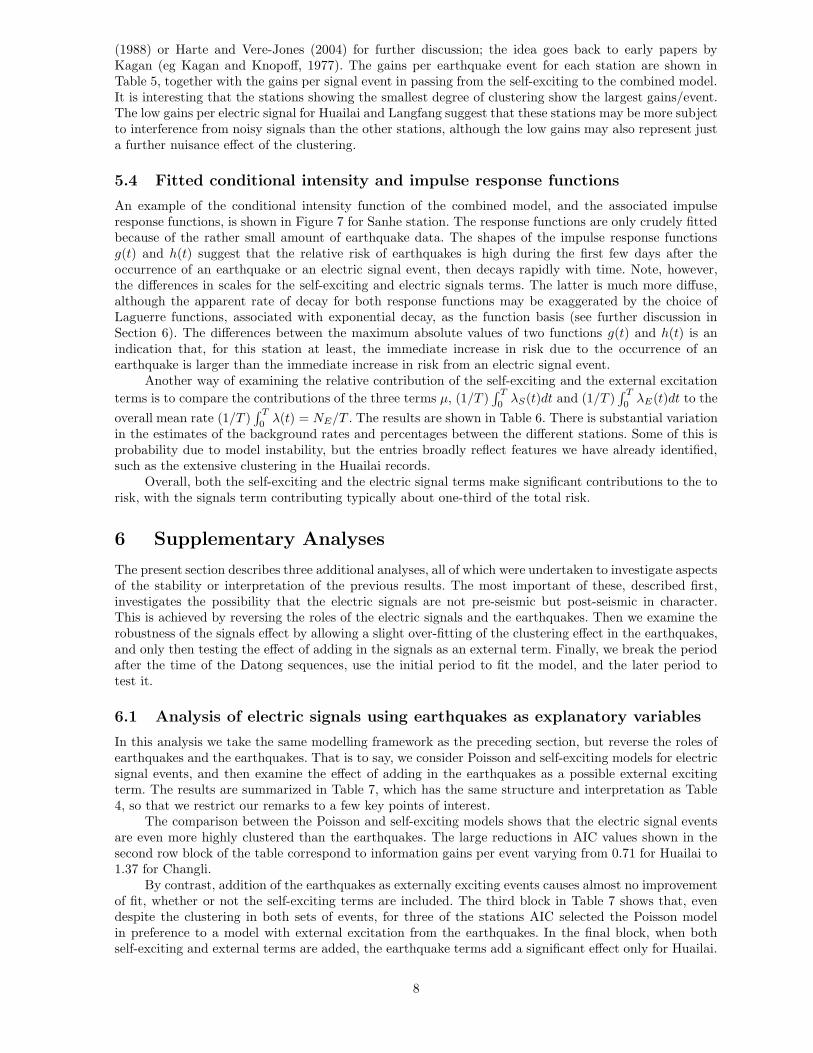
5.4 Fitted conditional intensity and impulse response functions

An example of the conditional intensity function of the combined model, and the associated impulseresponse functions, is shown in Figure 7 for Sanhe station. The response functions are only crudely fittedbecause of the rather small amount of earthquake data. The shapes of the impulse response functionsg(t) and h(t) suggest that the relative risk of earthquakes is high during the first few days after theoccurrence of an earthquake or an electric signal event, then decays rapidly with time. Note, however,the differences in scales for the self-exciting and electric signals terms. The latter is much more diffuse,although the apparent rate of decay for both response functions may be exaggerated by the choice ofLaguerre functions, associated with exponential decay, as the function basis (see further discussion inSection 6). The differences between the maximum absolute values of two functions g(t) and h(t) is anindication that, for this station at least, the immediate increase in risk due to the occurrence of anearthquake is larger than the immediate increase in risk from an electric signal event.

Another way of examining the relative contribution of the self-exciting and the external excitation

terms is to compare the contributions of the three terms µ, (1/T )∫ T

0λS(t)dt and (1/T )

∫ T

0λE(t)dt to the

overall mean rate (1/T )∫ T

0λ(t) = NE/T . The results are shown in Table 6. There is substantial variation

in the estimates of the background rates and percentages between the different stations. Some of this isprobability due to model instability, but the entries broadly reflect features we have already identified,such as the extensive clustering in the Huailai records.

Overall, both the self-exciting and the electric signal terms make significant contributions to the torisk, with the signals term contributing typically about one-third of the total risk.

6 Supplementary Analyses

The present section describes three additional analyses, all of which were undertaken to investigate aspectsof the stability or interpretation of the previous results. The most important of these, described first,investigates the possibility that the electric signals are not pre-seismic but post-seismic in character.This is achieved by reversing the roles of the electric signals and the earthquakes. Then we examine therobustness of the signals effect by allowing a slight over-fitting of the clustering effect in the earthquakes,and only then testing the effect of adding in the signals as an external term. Finally, we break the periodafter the time of the Datong sequences, use the initial period to fit the model, and the later period totest it.

6.1 Analysis of electric signals using earthquakes as explanatory variables

In this analysis we take the same modelling framework as the preceding section, but reverse the roles ofearthquakes and the earthquakes. That is to say, we consider Poisson and self-exciting models for electricsignal events, and then examine the effect of adding in the earthquakes as a possible external excitingterm. The results are summarized in Table 7, which has the same structure and interpretation as Table4, so that we restrict our remarks to a few key points of interest.

The comparison between the Poisson and self-exciting models shows that the electric signal eventsare even more highly clustered than the earthquakes. The large reductions in AIC values shown in thesecond row block of the table correspond to information gains per event varying from 0.71 for Huailai to1.37 for Changli.

By contrast, addition of the earthquakes as externally exciting events causes almost no improvementof fit, whether or not the self-exciting terms are included. The third block in Table 7 shows that, evendespite the clustering in both sets of events, for three of the stations AIC selected the Poisson modelin preference to a model with external excitation from the earthquakes. In the final block, when bothself-exciting and external terms are added, the earthquake terms add a significant effect only for Huailai.

8

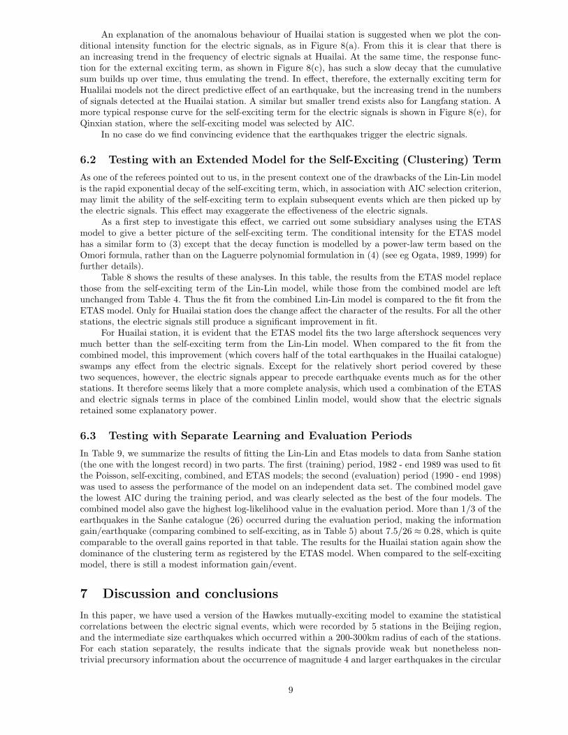
An explanation of the anomalous behaviour of Huailai station is suggested when we plot the con-ditional intensity function for the electric signals, as in Figure 8(a). From this it is clear that there isan increasing trend in the frequency of electric signals at Huailai. At the same time, the response func-tion for the external exciting term, as shown in Figure 8(c), has such a slow decay that the cumulativesum builds up over time, thus emulating the trend. In effect, therefore, the externally exciting term forHualilai models not the direct predictive effect of an earthquake, but the increasing trend in the numbersof signals detected at the Huailai station. A similar but smaller trend exists also for Langfang station. Amore typical response curve for the self-exciting term for the electric signals is shown in Figure 8(e), forQinxian station, where the self-exciting model was selected by AIC.

In no case do we find convincing evidence that the earthquakes trigger the electric signals.

6.2 Testing with an Extended Model for the Self-Exciting (Clustering) Term

As one of the referees pointed out to us, in the present context one of the drawbacks of the Lin-Lin modelis the rapid exponential decay of the self-exciting term, which, in association with AIC selection criterion,may limit the ability of the self-exciting term to explain subsequent events which are then picked up bythe electric signals. This effect may exaggerate the effectiveness of the electric signals.

As a first step to investigate this effect, we carried out some subsidiary analyses using the ETASmodel to give a better picture of the self-exciting term. The conditional intensity for the ETAS modelhas a similar form to (3) except that the decay function is modelled by a power-law term based on theOmori formula, rather than on the Laguerre polynomial formulation in (4) (see eg Ogata, 1989, 1999) forfurther details).

Table 8 shows the results of these analyses. In this table, the results from the ETAS model replacethose from the self-exciting term of the Lin-Lin model, while those from the combined model are leftunchanged from Table 4. Thus the fit from the combined Lin-Lin model is compared to the fit from theETAS model. Only for Huailai station does the change affect the character of the results. For all the otherstations, the electric signals still produce a significant improvement in fit.

For Huailai station, it is evident that the ETAS model fits the two large aftershock sequences verymuch better than the self-exciting term from the Lin-Lin model. When compared to the fit from thecombined model, this improvement (which covers half of the total earthquakes in the Huailai catalogue)swamps any effect from the electric signals. Except for the relatively short period covered by thesetwo sequences, however, the electric signals appear to precede earthquake events much as for the otherstations. It therefore seems likely that a more complete analysis, which used a combination of the ETASand electric signals terms in place of the combined Linlin model, would show that the electric signalsretained some explanatory power.

6.3 Testing with Separate Learning and Evaluation Periods

In Table 9, we summarize the results of fitting the Lin-Lin and Etas models to data from Sanhe station(the one with the longest record) in two parts. The first (training) period, 1982 - end 1989 was used to fitthe Poisson, self-exciting, combined, and ETAS models; the second (evaluation) period (1990 - end 1998)was used to assess the performance of the model on an independent data set. The combined model gavethe lowest AIC during the training period, and was clearly selected as the best of the four models. Thecombined model also gave the highest log-likelihood value in the evaluation period. More than 1/3 of theearthquakes in the Sanhe catalogue (26) occurred during the evaluation period, making the informationgain/earthquake (comparing combined to self-exciting, as in Table 5) about 7.5/26 ≈ 0.28, which is quitecomparable to the overall gains reported in that table. The results for the Huailai station again show thedominance of the clustering term as registered by the ETAS model. When compared to the self-excitingmodel, there is still a modest information gain/event.

7 Discussion and conclusions

In this paper, we have used a version of the Hawkes mutually-exciting model to examine the statisticalcorrelations between the electric signal events, which were recorded by 5 stations in the Beijing region,and the intermediate size earthquakes which occurred within a 200-300km radius of each of the stations.For each station separately, the results indicate that the signals provide weak but nonetheless non-trivial precursory information about the occurrence of magnitude 4 and larger earthquakes in the circular

9

region around the station. In the converse direction the results are equally unequivocal; in no case do theearthquakes appear to carry significant precursory information about the occurrence of the signal eventsrecorded at the station.

In response to concerns expressed by the referees and others who have commented on earlier draftsof this paper, we would like to make the following comments.

1. While it may be that the electric signals data analyzed in this study have been collected by relativelysimple equipment, and that the initial data handling requires a degree of subjective interventionand interpretation, the data analyzed are part of a systematic, standardized process of measurementand reporting that has been carried out in the Beijing region for the better part of twenty years.From the point where they have been collected by CAP, the data used are quantitative, objective,and available for analysis. Within CAP, they form a regular and integral part of the surveillanceand forecasting programme, and have done for many years.

2. During the period of the study, all five stations report very comparable effects, despite local vari-ations in seismicity and geological and man-made environment. Even if the observation period isbroken up into sections, similar effects are observed in each section, as outlined in section 6.3. Thegreatest deviations from the common pattern occur for Huailai station. Even here it seems likelythat the discrepancies are caused by the two large aftershock sequences which enter the earthquakesubcatalogue for this station, and that the discrepancies would be much reduced if the aftershockperiods were either better modelled in the combined model, or removed from the analysis.

3. The statistical analysis applied to this data is also crude. Information is lost in converting the signalsto 0-1 data, and only the simple Lin-Lin model has been used in the main analysis. Nevertheless itis sufficient to show that the precursory effect of the electrical signals persists even after allowancehas been made for earthquake clustering, and that the electric signals are pre- and not post-seismicin character. Interpretation of the AIC values and associated significance levels is subject to someuncertainty, but in most cases there is a large margin of error. The fact that similar significancelevels are recorded for all stations substantially increases the overall significance.

4. It is clear that in some cases the signals have been contaminated by the occurrence of electric storms,man-made electrical appliances, etc. Except in the most obvious cases, all such disturbances havebeen incorporated into the assessment of the daily strengths. In such a situation, unless the inter-fering signals carried predictive information similar to those of the anomalous signals themselves,one would expect them to act as noise and to decrease the apparent correlations between the signalsand earthquakes. Additional studies by Guan and coworkers suggest that in fact the majority ofthe observed signals are not related to interference from meteorological phenomena or magneticstorms. For example, the electric signals do not appear to reflect annual fluctuations in rainfall ortemperature (Guan et al, 1996), nor do the large-scale magnetic storms appear to be associated withmajor variations in either the electric signals or the earthquakes (ibid). As for man-made signals,the two sites most likely to be affected by these, namely Langfang and Huailai, both show increasedfrequency of electric signals with time, and are accompanied by rather low values of the predictivepower per signal. These features suggest that, for these stations at least, the earthquake-associatedsignals are indeed diluted by noise signals which build up as urbanization of the area increases. Atleast for the observation periods in the present study, however, these effects are not so large as todestroy the correlations with the earthquakes.

5. At present, we have no answer to what may be the most serious problem associated with the presenttopic, namely the absence of a plausible physical process that can explain the source and precursorycharacter of the electric signals. Our view here is that the existence of such a mechanism cannot yetbe ruled out, and that in such a situation the collection and presentation of empirical data, such asoutlined in the present study, is a necessary stage in the scientific process.

6. Although we are aware of the controversy which has surrounded earlier reports of links betweenground electric signals and earthquake occurrence, and the many serious criticisms which have beendirected towards some of these, we believe that the present data and analysis should be given theopportunity to be considered in their own right. At the least the data analyzed here summarize theresults of two decades of preparatory work which is unique of its kind in scale and consistency ofapplication.

10

In conclusion, we should emphasize that this is only a preliminary analysis of the data on electricsignals held by the China Seismological Bureau Centre of Analysis and Prediction. Its aim was to establishthat there is at least a prima facie case for taking seriously the claims that there may be a connectionbetween electric signals and earthquakes. At this point, we cannot fully exclude the possibility thatthe positive results obtained in this analysis have their roots in aspects of the data handling, selectionprocedures, and analysis, or in some coincidental relation between earthquake occurrence and man-madeor physical noise. Our belief, however, is that this is unlikely to be the case.

We should also emphasize that the present paper does not pretend to set up a quantitative forecastingscheme. It is based on a retrospective study of existing data, and leaves unresolved many issues relatingto the combination of information from the different stations, and the estimation of locations and sizesof possible future earthquakes, all of which would have to be resolved before a quantitative forecastingscheme could be put into place. Some of these aspects are pursued further in the companion study byZhuang et al (2002), which is currently available as a technical report; some part of its findings aresummarized in Ogata and Zhuang (2001).

At the present time, the electric signals stations around Beijing are in the process of being convertedto digital stations. When this process is completed, it should allow an unequivocal answer to be given toconcerns about reliability and objectivity of the data which have been raised. Should the results confirmthe findings in the present report, the existing data will be a unique source of information about theelectric signals, and their protection becomes a matter of both national and international importance.

Acknowledgements

We would like to acknowledge the critical but nonetheless helpful advice that we have received from theReferees (Yan Kagan and Francesco Mulargia), from Robert Davies, and from other colleagues, all of whichhave contributed substantially to improvements to the original draft of this paper. The work describedin the present study was initialized with assistance of No. 10371012 of the National Natural ScienceFoundation of China, then was surported primarily with partial assistance of a subcontract on earthquakeforecasting with the Institute of Geological and Nuclear Sciences on FRST Contract Natural Hazardsof New Zealand and Gran-in-Aid 11680334 for the Scientific Research from the Ministry of Education,Science, Sport and Culture, Japan. The observation part on the ground ULF electric signals by the fourthauthor has been supported by No. 2001BA601B01-05-03 of the 10th Five-Year-Term Scientific ResearchFunds of China Seismological Bureau. All of these financial assistance are gratefully acknowledged here.The writing of the paper was assisted by grants from the Centre for Mathematics and its Applicationsin Minneapolis.

References

Akaike, H. (1974), A New Look at the Statistical Model Identification, IEEE Transaction on AutomaticControl, AC-19, 716–723.

Chen, Z., Du, X., Song, R. and Guan H., Electromagnetic Radiation and Earthquakes (in Chinese),(Seismological Press, Beijing, 1998).

Chen, Z. and Xu, C., Features of Electric-Magnetic Radiation Between Some Shallow Earthquakes inNorth China, In Studies on New Method of Short-term Earthquake Prediction, (eds. Department ofMonitoring, State Seismology Bureau), (Seismological Press, Beijing, 1994).

Daley, D. and Vere-Jones, D., An Introduction to the Theory of Point Processes, Vol. 1. (2nd edition).(Springer, New York, 2002).

Guan, H. and Liu, G. (1995), Electromagnetic Radiation Anomalies Before Moderate and Strong Earth-quakes, Acta Seismologica Sinica, 9, 289–299.

Guan, H., Chen, Z. and Yu, S. (1996). Analysis on the Relationship Between Earthquakes and Electric-Magnetic Radiation, Earthquake Research in China, 16, 168–176.

Guan, H., Zhang, H., Liu, Y., Yu, S. and Chen, Z. (1999), Studies on the Relationship Between theAnomalies of the Ultra-Low Frequency Electric Field and Earthquakes (in Chinese with Englishabstract), Earthquake, 19, 142–148.

11

Guan, H., Chen, Z. and Yu, S. (2000), Study on Seismic Precursor Features of Electromagnetic Radiationin the Beijing Region and its Surrounding Area (In Chinese with English abstract), Earthquake,20, 65–70.

Harte, D. and Vere-Jones, D. (2004), The entropy score and its uses in earthquake forecasting, This

volume.

Hawkes, A. G. (1971), Spectra of Some Self-Exciting and Mutually Exciting Point Processes, Biometrika,58, 83–90.

Kagan, Y. Y. and Knopoff, L. (1977), Earthquake Risk Prediction as a Stochastic Process, Physics ofthe Earth and Planetary Interior, 14, 97–108.

Ma, L. and Vere-Jones, D. (1997), Application of M8 and Lin-Lin Algorithms to New Zealand EarthquakeData, New Zealand Journal of Geology and Geophysics, 35, 77–89.

Michael, A. (1997), Test Prediction Methods: Earthquake Clustering Versus the Poisson Model, Geo-physical Research Letters, 24, 1891–1894.

Ogata, Y., Akaike, H. and Katsura, K. (1982), The Application of Linear Intensity Models to the In-vestigation of Causal Relations Between a Point Process and Another Stochastic Process, Annals ofthe Institute of Statistical Mathematics, 34, 373–387.

Ogata, Y. (1983), Likelihood Analysis of Point Processes and its Application to Seismological data,Bulletin of the International Statistical Institute, 50, 943–961.

Ogata, Y. (1989), Statistical Model for Standard Seismicity and Detection of Anomalies by ResidualAnalysis for Point Process, Tectonophysics, 169, 1–16.

Ogata, Y., (1999), Seismicity Analysis Through Point-Process Modelling: A Review, Pure and AppliedGeophysics, 155, 471–507.

Ogata, Y. and Zhuang, J. (2001), Statistical examination of anomalies for the precursor to earthquakes,and the multi-element prediction formula: Hazard rate changes of strong earthquakes M ≥ 4.0around Beijing area based on the ultra-low frequency electric observation (1982-1997), Report ofthe Coordinating Committee for Earthquake Prediction, Geographical Survey Institute, Tsukuba,Japan, 66, 562–570.

Utsu, T. and Ogata, Y. (1997), Statistical analysis of seismicity. In Algorithm for Earthquake Statisticsand Prediction, IAPSPEI Software Library (International Association of Seismologigy and Physicsof the Earth’s Interior. 6, 13—94).

Vere-Jones, D. and Ozaki T. (1982), Some Examples of Statistical Estimation Applied to EarthquakeData , Annals of the Institute of Statistical Mathematics, 34, 189–207.

Vere-Jones, D. (1998), Probabilities and Information Gain for Earthquake Forecasting, ComputationalSeismology, 30, 248–263.

Zhuang, J., Ogata, Y., Vere-Jones, D., Ma, L. and Guan, H. (2002), Statistical confirmation of a relation-ship between excitation of the utra-low frequency electric signals and magnitude M ≥ 4 earthquakesin a 300 km radius region around Beijing, Research memorandum 847, Institute of Statistical Math-ematics, Tokyo, Japan.

12

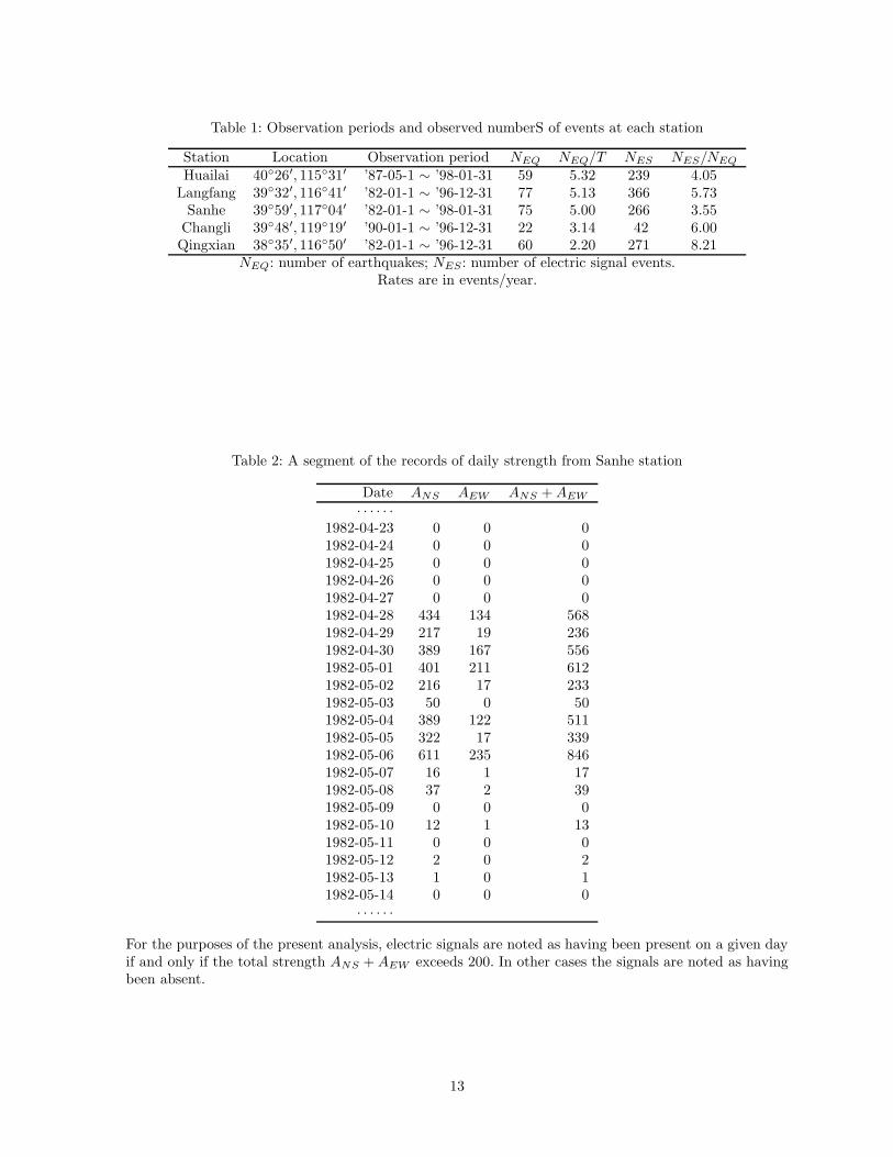
Table 1: Observation periods and observed numberS of events at each station

Station Location Observation period NEQ NEQ/T NES NES/NEQ

Huailai 40◦26′, 115◦31′ ’87-05-1 ∼ ’98-01-31 59 5.32 239 4.05Langfang 39◦32′, 116◦41′ ’82-01-1 ∼ ’96-12-31 77 5.13 366 5.73

Sanhe 39◦59′, 117◦04′ ’82-01-1 ∼ ’98-01-31 75 5.00 266 3.55Changli 39◦48′, 119◦19′ ’90-01-1 ∼ ’96-12-31 22 3.14 42 6.00Qingxian 38◦35′, 116◦50′ ’82-01-1 ∼ ’96-12-31 60 2.20 271 8.21

NEQ: number of earthquakes; NES : number of electric signal events.Rates are in events/year.

Table 2: A segment of the records of daily strength from Sanhe station

Date ANS AEW ANS + AEW

· · · · · ·1982-04-23 0 0 01982-04-24 0 0 01982-04-25 0 0 01982-04-26 0 0 01982-04-27 0 0 01982-04-28 434 134 5681982-04-29 217 19 2361982-04-30 389 167 5561982-05-01 401 211 6121982-05-02 216 17 2331982-05-03 50 0 501982-05-04 389 122 5111982-05-05 322 17 3391982-05-06 611 235 8461982-05-07 16 1 171982-05-08 37 2 391982-05-09 0 0 01982-05-10 12 1 131982-05-11 0 0 01982-05-12 2 0 21982-05-13 1 0 11982-05-14 0 0 0

· · · · · ·

For the purposes of the present analysis, electric signals are noted as having been present on a given dayif and only if the total strength ANS + AEW exceeds 200. In other cases the signals are noted as havingbeen absent.

13

Table 3: List of the earthquakes in this analysis. The coding inthe last columkn indicate the stations for which the given eventlay within one or other of the observation circles: H=Huailai, L= Langfang, S = Sanhe, C = Changli, Q = Qinxian. Lower suffix(eg H1) refers to smaller event within 200km radius. Upper suffix(1) refers to larger event in outer annulus (M > 5 between 200and 300km from station). Double suffix (1

1) refers to a larger event

within the smaller circle.

Date Time Latitude Longitude Magnitude Remark1982-01-20 14:54:13 37◦02′ 117◦32′ 4.2 Q1

1982-01-26 17:47:57 37◦24′ 114◦52′ 4.8 Q1

1982-01-27 12:30:42 39◦45′ 118◦46′ 4.4 S1C1

1982-02-09 17:33:37 39◦38′ 118◦09′ 4.7 L1S1C1

1982-03-08 03:41:59 39◦52′ 118◦40′ 4.9 S1C1

1982-03-30 12:06:33 39◦48′ 118◦30′ 4.2 S1C1

1982-07-09 17:18:24 38◦07′ 119◦23′ 4.1 C1

1982-08-09 04:07:11 38◦58′ 120◦35′ 4.0 C1

1982-10-19 20:46:01 39◦53′ 118◦59′ 5.3 L1S1C1

1

1982-12-10 02:16:46 40◦28′ 116◦33′ 4.9 H1L1S1

1983-01-31 01:50:03 37◦26′ 115◦01′ 4.1 L1Q1

1983-02-06 08:05:47 37◦31′ 114◦57′ 4.5 L1Q1

1983-04-03 10:16:30 40◦45′ 114◦47′ 5.1 H1

1L1

1983-07-21 05:55:55 40◦49′ 114◦42′ 4.4 H1

1983-08-03 14:21:15 37◦38′ 119◦06′ 4.4 C1

1983-08-08 09:04:58 40◦40′ 115◦23′ 4.1 H1L1

1983-08-21 05:00:31 39◦43′ 118◦19′ 4.1 S1C1

1983-08-26 17:22:18 39◦48′ 117◦13′ 4.3 H1L1S1C1

1983-09-09 22:12:45 40◦28′ 116◦34′ 4.0 H1L1S1

1983-09-15 12:18:35 37◦31′ 114◦16′ 4.1 Q1

1983-10-05 00:25:17 39◦51′ 118◦54′ 4.7 S1C1

1984-01-07 19:18:22 39◦43′ 118◦45′ 5.2 L1S1C1

1

1984-02-27 05:00:08 39◦26′ 118◦01′ 4.3 L1S1C1

1984-03-11 11:24:07 39◦38′ 118◦22′ 4.0 S1C1

1984-03-16 11:43:54 38◦28′ 119◦05′ 4.0 S1C1

1984-05-17 11:08:26 38◦58′ 119◦08′ 4.2 S1C1

1984-11-27 09:54:20 40◦30′ 114◦08′ 4.5 H1

1984-11-27 09:58:20 40◦29′ 114◦16′ 4.1 H1

1984-12-13 11:20:25 39◦39′ 118◦13′ 4.1 S1C1

1985-01-26 20:55:53 37◦22′ 114◦46′ 4.2 Q1

1985-04-22 11:31:33 39◦45′ 118◦46′ 5.0 L1S1C1

1

1985-04-22 19:02:37 39◦44′ 118◦47′ 4.3 S1C1

1985-04-22 19:56:59 39◦43′ 118◦46′ 4.7 S1C1

1985-05-22 18:51:44 39◦50′ 118◦32′ 4.7 S1C1

1985-08-11 01:17:16 39◦44′ 118◦45′ 4.0 S1C1

1985-08-11 01:30:32 39◦45′ 118◦47′ 4.5 S1C1

1985-08-11 02:29:15 39◦46′ 118◦46′ 4.0 S1C1

1985-08-23 23:19:31 39◦45′ 118◦45′ 4.0 S1C1

1985-08-25 17:05:19 39◦44′ 118◦30′ 4.4 S1C1

1985-10-05 12:01:58 39◦47′ 118◦27′ 5.0 H1L1S1

1C1

1Q1

1985-10-17 00:08:25 39◦17′ 114◦39′ 4.1 H1L1Q1

1985-11-21 19:42:22 40◦05′ 115◦50′ 4.7 H1L1S1

1985-11-23 08:47:14 38◦47′ 121◦11′ 4.5 C1

1985-11-30 22:38:00 37◦14′ 114◦49′ 5.6 L1S1Q1

1

1986-01-11 17:54:35 37◦26′ 114◦54′ 4.1 L1Q1

1986-02-05 17:18:36 39◦45′ 118◦26′ 4.0 S1C1

1986-02-15 07:08:47 37◦45′ 115◦14′ 4.8 L1Q1

14

Table 3: (continued)

Date Time Latitude Longitude Magnitude Remark1986-02-18 06:07:03 37◦48′ 115◦11′ 4.5 L1Q1

1986-07-02 11:56:58 38◦23′ 120◦29′ 4.6 C1

1986-07-02 11:58:29 38◦24′ 120◦30′ 4.3 C1

1986-11-10 16:58:05 40◦03′ 116◦43′ 4.7 H1L1S1

1986-12-16 07:25:56 37◦16′ 114◦45′ 4.2 Q1

1987-03-21 07:00:23 38◦17′ 114◦15′ 4.5 L1Q1

1987-05-22 11:50:42 40◦00′ 116◦47′ 4.0 H1L1S1

1987-06-07 12:26:23 39◦32′ 118◦05′ 4.5 L1S1C1

1987-07-16 02:16:28 39◦47′ 118◦38′ 4.5 S1C1

1987-08-08 07:35:06 39◦20′ 117◦53′ 4.7 L1S1C1

1987-08-08 17:35:08 39◦20′ 117◦54′ 4.1 L1S1C1

1987-11-11 21:18:39 40◦17′ 114◦48′ 4.7 H1L1

1988-05-09 06:22:01 39◦18′ 118◦06′ 4.2 L1S1C1

1988-07-23 13:51:43 40◦05′ 114◦13′ 5.0 H1

1L1

1S1Q1

1988-07-25 01:47:39 39◦31′ 118◦06′ 4.4 L1S1C1

1988-07-26 22:46:39 39◦34′ 118◦06′ 4.9 L1S1C1

1988-07-30 18:44:32 39◦46′ 118◦43′ 4.3 S1C1

1988-08-03 17:44:11 39◦36′ 118◦39′ 4.6 S1C1

1988-10-26 01:29:44 39◦52′ 118◦29′ 4.3 S1C1

1989-06-18 14:50:59 39◦40′ 118◦19′ 4.3 S1C1

1989-07-23 03:15:09 37◦22′ 115◦02′ 4.3 Q1

1989-10-05 11:55:35 39◦37′ 118◦15′ 4.2 S1C1

1989-10-18 22:57:23 39◦57′ 113◦50′ 5.7 H1

1L1S1Q1

1989-10-18 23:29:59 39◦57′ 113◦50′ 4.2 H1

1989-10-19 00:52:55 39◦57′ 113◦48′ 4.2 H1

1989-10-19 01:01:34 39◦57′ 113◦49′ 6.1 H1

1L1S1Q1

1989-10-19 01:09:43 39◦54′ 113◦46′ 4.0 H1

1989-10-19 01:11:17 39◦58′ 113◦49′ 5.1 H1

1L1S1Q1

1989-10-19 01:26:26 40◦00′ 113◦51′ 4.4 H1

1989-10-19 02:20:46 39◦59′ 113◦52′ 5.6 H1

1L1S1Q1

1989-10-19 05:02:03 39◦55′ 113◦49′ 4.4 H1

1989-10-19 18:29:03 39◦55′ 113◦44′ 5.1 H1

1L1S1Q1

1989-10-20 01:56:48 39◦56′ 113◦48′ 4.1 H1

1989-10-20 19:41:41 39◦59′ 113◦54′ 4.1 H1

1989-10-23 21:19:32 39◦55′ 113◦49′ 5.2 H1

1L1S1Q1

1989-10-29 10:22:43 39◦56′ 113◦49′ 4.1 H1

1989-12-09 07:04:51 39◦53′ 113◦49′ 4.2 H1

1989-12-13 09:10:11 39◦56′ 113◦53′ 4.1 H1

1989-12-14 12:13:01 37◦36′ 115◦17′ 4.8 L1Q1

1989-12-25 04:26:23 40◦20′ 118◦57′ 4.7 C1

1989-12-31 16:24:48 39◦58′ 113◦51′ 4.0 H1

1990-03-16 15:08:39 39◦46′ 118◦27′ 4.2 S1C1

1990-05-23 14:13:01 40◦13′ 116◦28′ 4.3 H1L1S1

1990-07-21 08:41:51 40◦35′ 115◦50′ 5.0 H1

1L1

1S1Q1

1990-07-23 16:41:32 39◦45′ 118◦29′ 4.9 S1C1

1990-08-03 18:05:44 37◦53′ 115◦02′ 4.2 L1Q1

1990-09-22 11:02:19 40◦05′ 116◦22′ 4.5 H1L1S1

1990-12-24 13:31:03 37◦54′ 115◦01′ 4.1 L1Q1

1991-01-29 06:28:04 38◦28′ 112◦32′ 5.5 H1

1991-03-26 02:02:38 39◦58′ 113◦51′ 6.1 H1

1L1S1Q1

1991-03-26 02:07:27 39◦59′ 113◦50′ 4.3 H1

1991-04-01 05:35:23 39◦54′ 113◦49′ 4.0 H1

1991-05-07 00:25:01 39◦48′ 118◦42′ 4.3 S1C1

1991-05-29 19:02:10 39◦43′ 118◦18′ 5.2 H1L1S1

1C1

1Q1

15

Table 3: (continued)

Date Time Latitude Longitude Magnitude Remark1991-05-30 07:06:55 39◦41′ 118◦16′ 5.6 H1L1S1

1C1

1Q1

1991-07-11 19:05:05 39◦41′ 118◦23′ 4.3 S1C1

1991-07-27 17:54:47 39◦51′ 118◦48′ 4.4 S1C1

1991-08-21 05:28:28 37◦20′ 114◦42′ 4.3 Q1

1991-08-22 06:23:37 37◦28′ 114◦44′ 4.1 Q1

1991-09-02 04:17:42 38◦49′ 119◦59′ 4.1 C1

1991-09-20 17:52:06 39◦20′ 114◦05′ 4.1 H1L1

1991-09-28 08:37:47 40◦05′ 117◦03′ 4.0 H1L1S1

1991-09-28 18:48:06 40◦04′ 117◦04′ 4.0 H1L1S1

1991-10-05 05:44:39 39◦18′ 117◦57′ 4.0 L1S1C1

1991-10-07 07:25:21 37◦56′ 115◦04′ 4.1 L1Q1

1991-10-17 02:19:42 39◦44′ 118◦25′ 4.3 S1C1

1992-02-14 17:08:43 39◦46′ 118◦26′ 4.4 S1C1

1992-07-22 05:43:02 39◦17′ 117◦56′ 4.9 L1S1C1

1993-06-14 03:01:00 37◦25′ 119◦56′ 4.1 C1

1993-08-30 07:27:59 39◦54′ 113◦49′ 4.1 H1

1993-08-30 08:13:38 39◦54′ 113◦49′ 4.0 H1

1993-09-27 15:44:16 39◦39′ 118◦42′ 4.0 S1C1

1993-11-18 07:05:09 39◦36′ 117◦27′ 4.4 L1S1C1

1994-10-04 15:54:17 39◦44′ 118◦26′ 4.0 S1C1

1994-12-23 13:13:40 40◦28′ 115◦33′ 4.3 H1L1

1995-06-27 09:39:51 38◦14′ 119◦28′ 4.0 C1

1995-07-20 20:51:23 40◦16′ 115◦26′ 4.1 H1L1S1

1995-10-06 06:26:53 39◦40′ 118◦20′ 5.4 H1L1S1

1C1

1Q1

1995-11-13 14:33:19 39◦22′ 113◦12′ 4.5 H1

1996-04-08 00:39:28 39◦51′ 118◦44′ 4.0 S1C1

1996-12-16 05:36:33 40◦10′ 116◦30′ 4.5 H1L1S1

1996-12-16 09:52:24 40◦06′ 116◦35′ 4.0 H1L1S1

1997-04-12 15:05:02 38◦17′ 120◦29′ 4.3 C1

1997-05-25 14:59:08 40◦42′ 114◦52′ 4.7 H1

1998-01-10 11:50:39 41◦06′ 114◦18′ 6.2 H1

1L1

1998-01-10 11:59:17 41◦20′ 114◦32′ 4.0 H1

1998-01-10 12:09:58 41◦06′ 114◦28′ 4.5 H1

1998-01-10 13:03:59 41◦05′ 114◦30′ 4.6 H1

1998-01-10 15:38:18 41◦09′ 114◦32′ 4.2 H1

1998-01-10 20:01:55 41◦07′ 114◦26′ 4.0 H1

1998-01-10 21:50:32 41◦11′ 114◦26′ 4.3 H1

1998-01-10 23:33:20 41◦04′ 114◦25′ 4.0 H1

1998-01-11 02:37:47 41◦05′ 114◦25′ 4.6 H1

1998-01-11 11:31:43 41◦05′ 114◦26′ 4.4 H1

1998-01-12 02:41:54 41◦08′ 114◦27′ 4.3 H1

1998-01-12 18:32:29 41◦12′ 114◦28′ 4.3 H1

1998-01-14 01:17:26 41◦04′ 114◦27′ 4.2 H1

1998-01-14 11:09:57 41◦11′ 114◦31′ 4.3 H1

1998-01-17 10:41:18 41◦06′ 114◦26′ 4.3 H1

1998-01-18 04:07:25 41◦09′ 114◦22′ 4.6 H1

1998-01-18 06:17:54 41◦07′ 114◦28′ 4.3 H1

1998-01-22 12:11:51 41◦08′ 114◦26′ 4.4 H1

1998-01-27 07:29:07 41◦02′ 114◦29′ 4.2 H1

1998-02-13 07:05:05 41◦03′ 114◦27′ 4.0 H1

1998-04-14 10:47:48 39◦41′ 118◦28′ 5.0 H1L1S1

1C1

1Q1

1998-04-14 10:48:06 39◦41′ 118◦28′ 4.4 S1C1

1998-04-16 07:13:44 41◦05′ 114◦27′ 4.0 H1

1998-06-02 09:32:04 41◦11′ 114◦24′ 4.8 H1

16

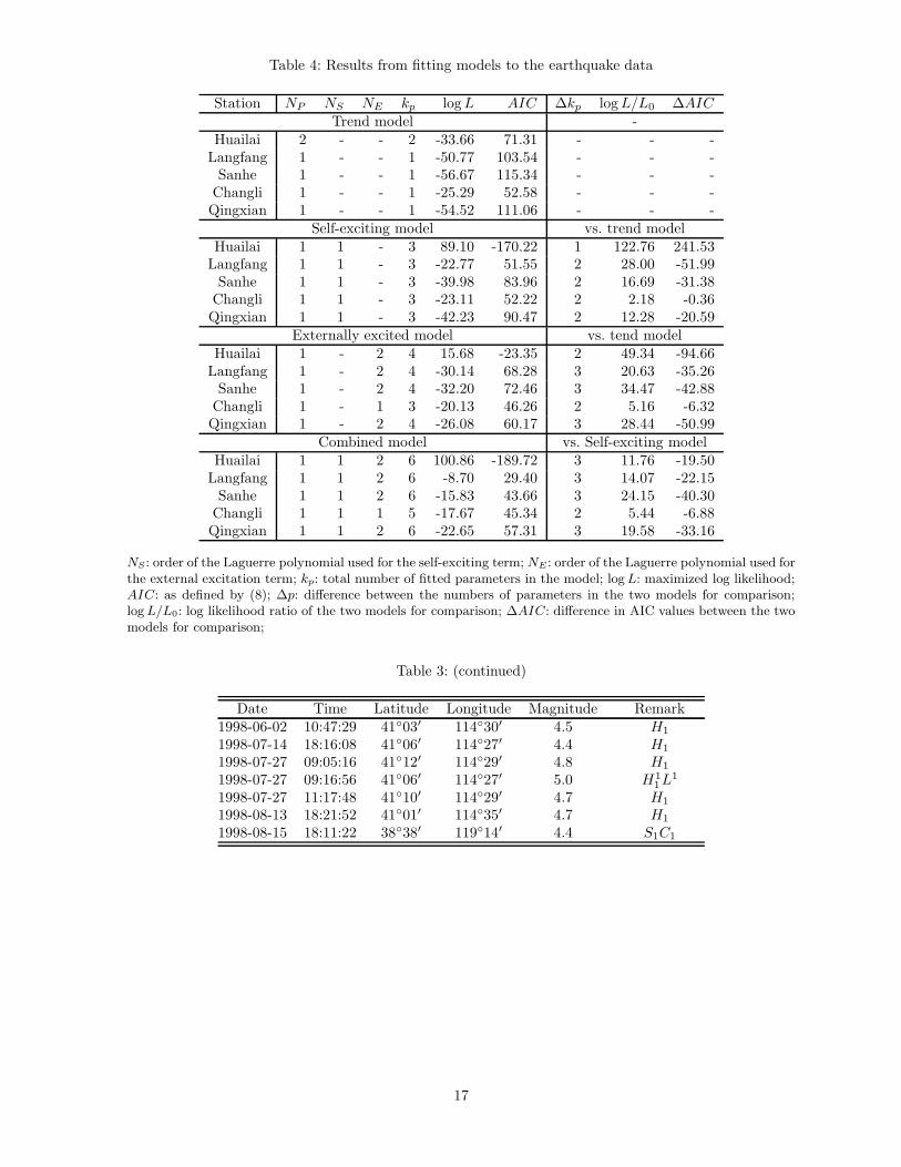
Table 4: Results from fitting models to the earthquake data

Station NP NS NE kp log L AIC ∆kp log L/L0 ∆AICTrend model -

Huailai 2 - - 2 -33.66 71.31 - - -Langfang 1 - - 1 -50.77 103.54 - - -

Sanhe 1 - - 1 -56.67 115.34 - - -Changli 1 - - 1 -25.29 52.58 - - -Qingxian 1 - - 1 -54.52 111.06 - - -

Self-exciting model vs. trend modelHuailai 1 1 - 3 89.10 -170.22 1 122.76 241.53

Langfang 1 1 - 3 -22.77 51.55 2 28.00 -51.99Sanhe 1 1 - 3 -39.98 83.96 2 16.69 -31.38

Changli 1 1 - 3 -23.11 52.22 2 2.18 -0.36Qingxian 1 1 - 3 -42.23 90.47 2 12.28 -20.59

Externally excited model vs. tend modelHuailai 1 - 2 4 15.68 -23.35 2 49.34 -94.66

Langfang 1 - 2 4 -30.14 68.28 3 20.63 -35.26Sanhe 1 - 2 4 -32.20 72.46 3 34.47 -42.88

Changli 1 - 1 3 -20.13 46.26 2 5.16 -6.32Qingxian 1 - 2 4 -26.08 60.17 3 28.44 -50.99

Combined model vs. Self-exciting modelHuailai 1 1 2 6 100.86 -189.72 3 11.76 -19.50

Langfang 1 1 2 6 -8.70 29.40 3 14.07 -22.15Sanhe 1 1 2 6 -15.83 43.66 3 24.15 -40.30

Changli 1 1 1 5 -17.67 45.34 2 5.44 -6.88Qingxian 1 1 2 6 -22.65 57.31 3 19.58 -33.16

NS : order of the Laguerre polynomial used for the self-exciting term; NE : order of the Laguerre polynomial used forthe external excitation term; kp: total number of fitted parameters in the model; log L: maximized log likelihood;AIC: as defined by (8); ∆p: difference between the numbers of parameters in the two models for comparison;log L/L0: log likelihood ratio of the two models for comparison; ∆AIC: difference in AIC values between the twomodels for comparison;

Table 3: (continued)

Date Time Latitude Longitude Magnitude Remark1998-06-02 10:47:29 41◦03′ 114◦30′ 4.5 H1

1998-07-14 18:16:08 41◦06′ 114◦27′ 4.4 H1

1998-07-27 09:05:16 41◦12′ 114◦29′ 4.8 H1

1998-07-27 09:16:56 41◦06′ 114◦27′ 5.0 H1

1L1

1998-07-27 11:17:48 41◦10′ 114◦29′ 4.7 H1

1998-08-13 18:21:52 41◦01′ 114◦35′ 4.7 H1

1998-08-15 18:11:22 38◦38′ 119◦14′ 4.4 S1C1

17

Table 5: Information gains per earthquake and per signal for each station

Station Infogain/earthquake Infogain/earthquake Infogain/signal(cluster v Poisson) (combined v cluster) (combined v cluster)

Huailai 2.08 0.20 0.049Langfang 0.36 0.18 0.038

Sanhe 0.22 0.28 0.091Changli 0.10 0.25 0.130Qingxian 0.20 0.33 0.072

The information gain means here the log-likelihood ratio, normalized bydividing by the number of earthquake events or the number of signal events.

Table 6: Comparison of intensities in the combined model.

Station µ Background Clustering Signals∫ T

0λEdt/NS

Huailai 0.3104 20.6% 50.8% 28.6% 0.071Langfang 0.7601 57.2% 14.9% 27.9% 0.056

Sanhe 0.6814 53.4% 10.5% 36.2% 0.102Changli 0.4143 48.1% 29.7% 22.2% 0.116Qingxian 0.4084 37.3% 15.7% 47.1% 0.104

µ is the estimated background rate in events per 100 days; the next three columns give percentages ofthe total rate due to each term in the intensity; the final column is a rough indication of the number of

predicted earthquakes per electric signal.

Table 7: Results from fitting models to the electric signals data

St. NP NS NE kp log L AIC ∆p log L/L0 ∆AICPoisson model -

Huailai 2 - - 2 195.23 -386.46 - - -Langfang 2 - - 2 479.90 -955.79 - - -

Sanhe 1 - - 1 135.76 -269.52 - - -Changli 1 - - 1 -21.12 44.25 - - -Qingxian 1 - - 1 162.32 -322.65 - - -

Self-exciting model vs. Trend modelHuailai 2 1 - 4 378.04 -748.08 2 182.81 -361.62

Langfang 2 1 - 4 741.20 -1474.40 2 261.30 -518.61Sanhe 1 2 - 4 384.47 -760.94 3 248.71 -491.42

Changli 1 1 - 3 28.45 -50.90 2 49.57 -95.15Qingxian 1 2 - 4 433.99 -859.98 3 271.67 -537.33

Externally excited model vs. Trend modelHuailai 1 - 3 5 221.16 -432.32 3 25.93 -45.86

Langfang 2 - 1 4 483.47 -958.95 2 3.57 -3.16Sanhe 1 - 3 5 137.58 -267.16 4 1.82 2.36

Changli 1 - 1 3 -21.12 48.25 2 0.00 4.00Qingxian 1 - 9 11 198.01 -334.01 10 35.69 -11.36

Combined model vs. Self-exciting modelHuailai 1 2 2 7 391.29 -768.59 3 13.25 -20.51

Langfang 2 1 1 6 741.20 -1470.40 2 0.00 4.00Sanhe 1 2 1 6 384.65 -757.30 2 0.18 3.64

Changli 1 1 1 5 30.34 -50.68 2 1.89 0.22Qingxian 1 2 2 7 434.56 -857.13 3 0.57 2.85

NS : order of the Laguerre polynomial used for the clustering term; NE : order of the Laguerre polynomial usedfor the external excitation term; kp: total number of fitted parameters in the model; log L: maximized logarithmlikelihood; AIC: as defined by (8); ∆p: difference between the numbers of parameters in the two models; log L/L0:logarithm likelihood ratio of the two models; ∆AIC: difference in AIC values between the two models.

18

Table 8: Fitting results from the ETAS model

Station µ K c α p log L AIC AICl

Huailai 0.3346 0.002340 0.0001442 2.608 1.088 120.2 -230.4 -189.72Langfang 1.008 0.006772 0.004906 1.012 1.200 -16.73 43.45 29.40

Shanhe .8576 0.02022 0.0007426 0.3438 1.094 -35.64 81.28 43.66Changli 0.7429 0.01807 0.01675 0.0000 1.423 -28.10 66.20 59.62

Qingxian 0.8161 0.005854 0.02902 0.2707 2.029 -42.32 94.63 57.31

AICl represent the AIC-values for the corresponding best combined model in Table 4.

Table 9: Training and evaluation

SanheTraining (NEQ = 49) Prediction (NEQ = 26)1982.1.1 – 1989.12.31 1990.1.1 – 1998.1.31

Model log L AIC log LCombined 0.87 10.26 -23.67

Self-exciting -11.07 28.15 -31.20ETAS -8.99 27.98 -29.08Poisson -23.67 49.34 -36.01

HuailaiTraining (NEQ = 23) Prediction(NEQ = 36)1982.1.1 – 1990.12.31 1991.1.1 – 1998.1.31

Model log L AIC log LCombined 43.18 -74.35 48.18

Self-exciting 38.16 -70.32 48.54ETAS 56.90 -103.80 60.37Poisson -10.59 23.18 -24.95

19

112 114 116 118 120 122

3637

3839

4041

4243

Latitude

Long

itude

BeijingL

S

Q

H

C

Figure 1: Distribution of earthquakes and electric signals observation stations around Beijing. Observationstations are denoted by black squares, with station initial inside. The two circles represent 200- and 300kmcircles around Lanfang station. Earthquakes are represented by small circles. The diameter correspondsto size of event, from ML = 4 for smallest to ML = 6.7 for largest. Dark circles denote events whichfell within the observation region for at least one station; light circles denote other events with similarmagnitudes. The Tangshan area is to the East, adjacent to the Changli station. The Datong and Zhangbeiaftershock sequences are the clusters to the S.W and N.W. of Huailai station, respectively.

20

(a)

(b)

(c)

Figure 2: (a) A general circuit diagram for the observation equipment; (b) A photograph of the electrodesand the DJ-1 recorder. The body of the sensor of the electrodes is made of high quality Cr18Ni9C stainlesssteel. The water-proof pipe (white) will cover the whole screened transmission cables (black) when theelectrodes are installed; (c) The DJ-1 recorder.

21

Periods in seconds

Res

pons

e

0.05 0.2 1 5 20

0.01

0.05

0.2

0.5

1

Figure 3: The observation system response function.

Figure 4: A photocopy of an original record. The fluctuations in the upper part of the chart are typical ofthe observed anomalous signals. The large pulse in the lower half of the chart is an example of a clearlydistinguishable interference pulse, not included in the computation of the daily signal strength.

22

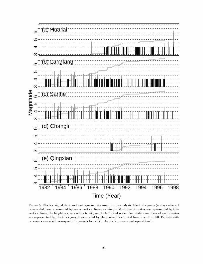
34

56

34

56

34

56

34

56

1982 1984 1986 1988 1990 1992 1994 1996 1998

Time (Year)

Mag

nitu

de(a) Huailai

(b) Langfang

(c) Sanhe

(d) Changli

(e) Qingxian

34

56

Figure 5: Electric signal data and earthquake data used in this analysis. Electric signals (ie days where 1is recorded) are represented by heavy vertical lines reaching to M=4. Earthquakes are represented by thinvertical lines, the height corresponding to ML on the left hand scale. Cumulative numbers of earthquakesare represented by the thick grey lines, scaled by the dashed horizontal lines from 0 to 80. Periods withno events recorded correspond to periods for which the stations were not operational.

23

(a)

(b)

Figure 6: A photocopy of a record with noises (the upper panel) from ground strong lightnings and (thebottom panel) from electricity leaked by power lines. In the upper panel, the short vertical bars, whichform up a line intersecting the horizontal line, are the timing marks at every minute, and irregular pulsescaused by strong ground lightnings are marked by arrows. In bottom, the part in black represent theperiod of power leakage.

24

Time (Year)

(a)E

vent

s/da

y

00.

30.

60.

91.

2

1982 1984 1986 1988 1990 1992 1994 1996 1998

Time (Year)

(b)

Eve

nts/

day

00.

30.

60.

91.

2

1989 1990 1991

0.00 0.05 0.10 0.15

010

2030

4050

Time (/100 days)

(c)

Eve

nts/

100d

ays

0.00 0.05 0.10 0.15

0.0

0.4

0.8

1.2

Time (/100 days)

(d)

Eve

nts/

100d

ays

Figure 7: Fitting results for the earthquake data around the Sanhe station using the ULF electric signalevents as explanatory factors. Top: Conditional intensity function throughout the whole time period;Middle: Conditional in a short period; Bottom left: impulse response from self excitation; Bottom right:impulse response from mutual excitation.

25

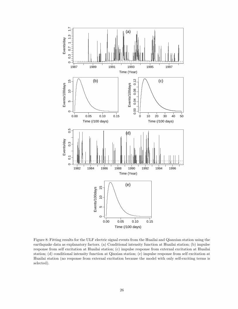
Time (Year)

Eve

nts/

day

00.

30.

71

1.3

1.7

1987 1989 1991 1993 1995 1997

(a)

0.00 0.05 0.10 0.15

05

1015

Time (/100 days)

Eve

nts/

100d

ays

(b)

0 10 20 30 40 50

0.00

0.04

0.08

0.12

Time (/100 days)

Eve

nts/

100d

ays

(c)

Time (Year)

Eve

nts/

day

(d)

00.

10.

30.

5

1982 1984 1986 1988 1990 1992 1994 1996

0.00 0.05 0.10 0.15

05

1015

Time (/100 days)

Eve

nts/

100d

ays

(e)

Figure 8: Fitting results for the ULF electric signal events from the Huailai and Qianxian station using theearthquake data as explanatory factors. (a) Conditional intensity function at Huailai station; (b) impulseresponse from self excitation at Huailai station; (c) impulse response from external excitation at Huailaistation; (d) conditional intensity function at Qinxian station; (e) impulse response from self excitation atHuailai station (no response from external excitation because the model with only self-exciting terms isselected).

26

REGISTRATION

of

Research Memorandum

Research Memorandum NO. 916 ; Received on(month)

06 ,(day)

14 ,(year)2004

by

Center for Information on Statistical Sciences

the Institute of Statistical Mathematics

(

Applicant: Zhuang Jiancangphone: 03-5421-8780, email: zhuangjc@ism.ac.jp

)

· · · · · · · · · · · · · · · · · · · · · · · · · · · · · · · · · · · · · · · · · · · · · · · · · · · · · · · · · · · · · · · · · · · · · · · · · · · · · · · · · · · · ·

Title:

Preliminary Analysis of Observations on the Ultra-Low Frequency ElectricField in a Region around Beijing

Author(Affiliation):

Zhuang, Jiancang (Institute of Statistical Mathematics, 106-8569, Tokyo,Japan);Vere-Jones, David (School of Mathematical and Computing Sciences, VictoriaUniversity of Wellington, PO Box 600, Wellington, New Zealand);Guan, Huaping (Center for Analysis and Prediction, China Seismological Bu-reau, 100036, Beijing, China);Ogata, Yosihiko (Institute of Statistical Mathematics, 106-8569, Tokyo, Japan);Ma, Li (Center for Analysis and Prediction, China Seismological Bureau,100036, Beijing, China)

Key words:

ultra-low frequency electric signal; earthquake; precursor; self-exciting andmutually exciting model

Abstract:

This paper presents a preliminary analysis of observations on ultra-lowfrequency ground electric signals from stations operated by the China Seismo-logical Bureau over the last 20 years. A brief description of the instrumenta-tion, operating procedures and data processing procedures is given. The dataanalysed consists of estimates of the total strengths (cumulated amplitudes) ofthe electric signals during 24 hour periods. The thresholds are set low enoughso that on most days a zero observation is returned. Non-zero observationsare related to electric and magnetic storms, occasional man-made electricaleffects, and, apparently, some pre-, co-, or post-seismic signals. The main

—to be continued —

Registration page 1

— continued —

purpose of the analysis is to investigate the extent that the electric signalscan be considered as pre-seismic in character. For this purpose the electricsignals from each of five stations are jointly analyzed with the catalogue oflocal earthquakes within circular regions around the selected stations. A ver-sion of Ogata’s Lin-Lin algorithm is used to estimate and test the existence ofa pre-seismic signal. This model allows the effect of the electric signals to betested, even after allowing for the effects of earthquake clustering. It is foundthat, although the largest single effect influencing earthquake occurrence isthe clustering tendency, there remains a significant preseismic componentfrom the electrical signals. Additional tests show that the apparent effect isnot post-seismic in character, and persists even under variations of the modeland the time periods used in the analysis. Samples of the data are presented,and the full data sets have been made available on local websites.

Registration page 2