Preliminary Analysis of Observations on the Ultra-Low Frequency

Electric Field in the Beijing Region

JIANCANG ZHUANG,1 DAVID VERE-JONES,2 HUAPING GUAN,3 YOSIHIKO OGATA,1 and

LI MA3

Abstract—This paper presents a preliminary analysis of observations on ultra-low frequency ground

electric signals from stations operated by the China Seismological Bureau over the last 20 years. A brief

description of the instrumentation, operating procedures and data processing procedures is given. The data

analyzed consists of estimates of the total strengths (cumulated amplitudes) of the electric signals during

24-hour periods. The thresholds are set low enough so that on most days a zero observation is returned.

Non-zero observations are related to electric and magnetic storms, occasional man-made electrical effects,

and, apparently, some pre-, co-, or postseismic signals. The main purpose of the analysis is to investigate

the extent that the electric signals can be considered as preseismic in character. For this purpose the electric

signals from each of five stations are jointly analyzed with the catalogue of local earthquakes within

circular regions around the selected stations. A version of Ogata’s Lin-Lin algorithm is used to estimate

and test the existence of a pre-seismic signal. This model allows the effect of the electric signals to be tested,

even after allowing for the effects of earthquake clustering. It is found that, although the largest single

effect influencing earthquake occurrence is the clustering tendency, there remains a significant preseismic

component from the electrical signals. Additional tests show that the apparent effect is not postseismic in

character, and persists even under variations of the model and the time periods used in the analysis.

Samples of the data are presented and the full data sets have been made available on local websites.

Key words: Ultra-low frequency electric signal, earthquake risk, Hawkes’ self-exciting and mutually

exciting model, Beijing.

1. Introduction

Systematic studies on the ground electric field as a source of possible earthquake

precursors were started in China following reports of substantial electric anomalies

before the MS7:8 Tangshan earthquake in 1976. Since that time more than 100

stations have been built in China to observe the ground electric field. Initially,

1 Institute of Statistical Mathematics, 4-6-7 Minami Azabu, Minato-Ku, Tokyo, 106-8569, Japan2 School of Mathematical and Computer Science, Victoria University of Wellington, P.O. Box 600

Wellington, New Zealand3 Center for Analysis and Prediction, China Seismological Bureau, 63 Fuxing Road, Beijing, 100036,

China

Pure appl. geophys. 162 (2005) 1367–13960033 – 4553/05/071367 – 30DOI 10.1007/s00024-004-2674-3

� Birkhauser Verlag, Basel, 2005

Pure and Applied Geophysics

observations were made over the whole frequency band. Experience showed that

observations on specific frequency bands, particularly the frequencies from 0.1 to 20

Hz, were most effective and best able to avoid contamination by industrial noise. In

1981, construction began on an ultra-low-frequency (ULF) observational network in

the Beijing region, using a frequency band of 0.1–10 Hz. The first stations from this

network started operation in 1982, while others were added during the ensuing

decade. The main purpose of this paper is to provide a preliminary statistical analysis

of accumulated data from the stations in this network.

Earlier studies of the electric signals data, of a more informal character and

involving stations from entire China, were made by CHEN and XU (1994), GUAN and

LIU (1995), and GUAN et al. (1996, 1999, 2000). They suggested that anomalous

fluctuations of the ultra-low frequency electric field may occur up to twenty days

before a relatively large earthquake in a neighborhood of the future focal region, and

that the characteristics of the anomalies may be related to the distance of the

recording station from the epicenter, and the magnitude of the coming earthquake.

This paper concentrates on data from five selected stations in the Beijing network,

and uses a statistical model to quantify the correlations between the occurrence of

anomalous fluctuations in the electric field and the occurrence of local earthquakes.

The earthquake data used in this study are listed at the end of the paper, and were

extracted from the China National Catalogue. A sample of the electric field data used

in this study is also listed at the end of the paper; the full set, together with the

earthquake data, is available from the website http://www.ism.ac.jp/�ogata/RM916/

Data.

In the following sections, we first give a brief account of the observational

equipment and operating procedures used by stations in the network (Section 2).

This is followed in Section 3 by an outline of the procedures used to obtain the

earthquake and electric signals data in the form used in the analysis. Section 4

describes the main statistical model used, which is applied in Sections 5 and 6 to data

from the five selected stations. The model is used to check the presence of both pre-

and postseismic effects, and allows for the effects of earthquake clustering. Section 6

also outlines some supplementary analyses designed to check internal consistency

and other features. The final section sets out the main conclusions of the paper.

2. Observation Network and Equipment

The electric signals observation network, from which the data for the present

study were taken, is located in a broad region around Beijing: see Figure 1. It was

started in 1981 with the aim of monitoring fluctuations in the electro-magnetic

radiations at frequencies in the 0.1–10 Hz (ULF) frequency band. The station

locations were chosen to avoid, as far as possible, man-made sources of interference

from electric railways, highways, underground metal pipes, power transformer

1368 J. Zhuang et al. Pure appl. geophys.,

substations, high-voltage power lines, areas of high energy consumption, radio

stations and power lines with ground connections. At the same time they were

selected to be close to known seismic belts or active faults. Eight stations are

currently operating in this network, from which the five stations with the longest and

highest quality records were selected for the present study. The locations of the

selected stations, namely Langfang, Sanhe, Qingxian, Huailai and Changli, are also

shown in Figure 1. Langfang, Sanhe, and Qingxian stations were set up in 1981–

1982, Huailai in 1987, and Changli in 1990.

The equipment and observation systems are similar at all the above stations. They

use the E-EM system designed by the Provincial Seismological Bureau of Hebei. We

provide only a brief description here, referring to CHEN and XU (1994) and CHEN

et al. (1998) for more detailed illustrations and technical parameters of the operating

systems.

The basic structure of the E-EM system is shown in Figure 2(a). It uses HBEMD-

3 type sensors (see CHEN et al. 1998) to detect the electric signals. To reduce the

effects of polarization potential, the electrodes of the sensor are made of high-quality

stainless steel (Cr18Ni9C), and are cylinder shaped with a height of 300 mm and a

radius of 4 mm; see Figure 2(b). In addition, 1000 l Farad capacitors are connected

in series into the system at each station, to eliminate direct currents.

112 114 116 118 120 122

3637

3839

4041

4243

Latitude

Long

itude

BeijingL

S

Q

H

C

Figure 1

Distribution of earthquakes and electric signals observation stations around Beijing. Observation stations

are denoted by black squares, with station initial inside. The two circles represent 200- and 300-km circles

around the Lanfang station. Earthquakes are represented by small circles. The diameter corresponds to

size of event, from ML ¼ 4 for smallest to ML ¼ 6:7 for largest. Dark circles denote events which fell within

the observation region for at least one station; light circles denote other events with similar magnitudes.

The Tangshan area is to the east, adjacent to the Changli station. The Datong and Zhangbei aftershock

sequences are the clusters to the southwest and northwest of the Huailai station, respectively.

Vol. 162, 2005 Analysis of Observations on the Ultra-Low Frequency Electric Field 1369

At each station, two pairs of electrodes are installed along perpendicular axes.

The electrodes are buried from 6 meters to 12 meters deep, and some 40 meters apart.

The electric signals detected by the sensor are transmitted to the preprocessor for

preliminary noise reduction, and then to the recorder. All wires used for signal

transmission are screened by high quality metal nets, covered by water-proof pipes,

and buried 0.6–0.8 meters below the surface. They go directly to the laboratory from

underground, and it is checked that no power supply wires, communication cables or

metal blocks are present nearby before operation commences.

The preprocessor includes an impedance matching unit and filter. Its main

functions are to prevent any 50 Hz noise produced by industrial power supplies from

Figure 2

A photograph of the electrodes and the DJ-1 recorder. The body of the sensor of the electrodes is made of

high quality Cr18Ni9C stainless steel. The water-proof pipe (white) will cover the whole screened

transmission cables (black) when the electrodes are installed. The top figure shows a general circuit

diagram for the observation equipment.

1370 J. Zhuang et al. Pure appl. geophys.,

coming into the amplifier, and to prevent the polarization potential from changing

the working point of the amplifier.

The signals are then fed to the amplifier to activate the recorder pen. The

recorders used (shown in Fig. 2(c)) are a modification of the DJ-1 recorder, originally

designed for recording the medium-long period components (0–10 Hz) of ground

movement with the DK-1 seismometer. These recorders and seismometers are widely

used at Chinese seismological stations. The recording method is by automatic

continuous pen record.

In order to improve the power supply quality, a stabilization plant is used for the

electricity supply instead of the usual commercial power supply. Power from

automatically recharged batteries is used when the power from the stabilization plant

is cut off. In addition, dual T bandpass filters, together with impedance matching

methods, are used to filter out any 50 Hz signals deriving from local power supplies

or other sources.

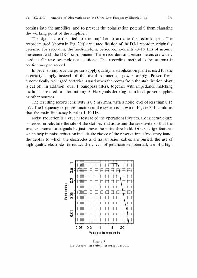
The resulting record sensitivity is 0.5 mV/mm, with a noise level of less than 0.15

mV. The frequency response function of the system is shown in Figure 3. It confirms

that the main frequency band is 1–10 Hz.

Noise reduction is a crucial feature of the operational system. Considerable care

is needed in selecting the site of the station, and adjusting the sensitivity so that the

smaller anomalous signals lie just above the noise threshold. Other design features

which help in noise reduction include the choice of the observational frequency band,

the depths to which the electrodes and transmission cables are buried, the use of

high-quality electrodes to reduce the effects of polarization potential, use of a high

Periods in seconds

Res

pons

e

0.05 0.2 1 5 20

0.01

0.05

0.2

0.5

1

Figure 3

The observation system response function.

Vol. 162, 2005 Analysis of Observations on the Ultra-Low Frequency Electric Field 1371

input resistance, screening of all transmission cables, filtering out 50 Hz noise, and

power-supply stabilization. Even despite these efforts, the existing stations differ

considerably in their ability to pick up or distinguish the anomalous signals.

3. Data

3.1 Electric Signals Data

The data used for the present analysis are the list of signal strengths, as reported

each day from each of the electric signals stations to the Centre for Analysis and

Prediction in Beijing. As already mentioned, the five stations for the present study,

chosen on the basis of the quality and completeness of their records, are Huailai,

Changli, Sanhe, Qingxian and Langfang. Because the stations were set up at different

times, and operated continuously over different periods, the observation time

intervals for these stations are different and are set out in detail in Table 1.

The signal strengths are determined on a daily basis according to the following

protocol, which was established at the beginning of the observation period, and is

observed in the same manner at each station. Each day, the drum record for each

pair of electrodes is examined for the presence of anomalies. The threshold of the

observing system is set low enough so that on most days the recording is close to a

horizontal line (zero). Typically, the anomalous signals do not occur continuously

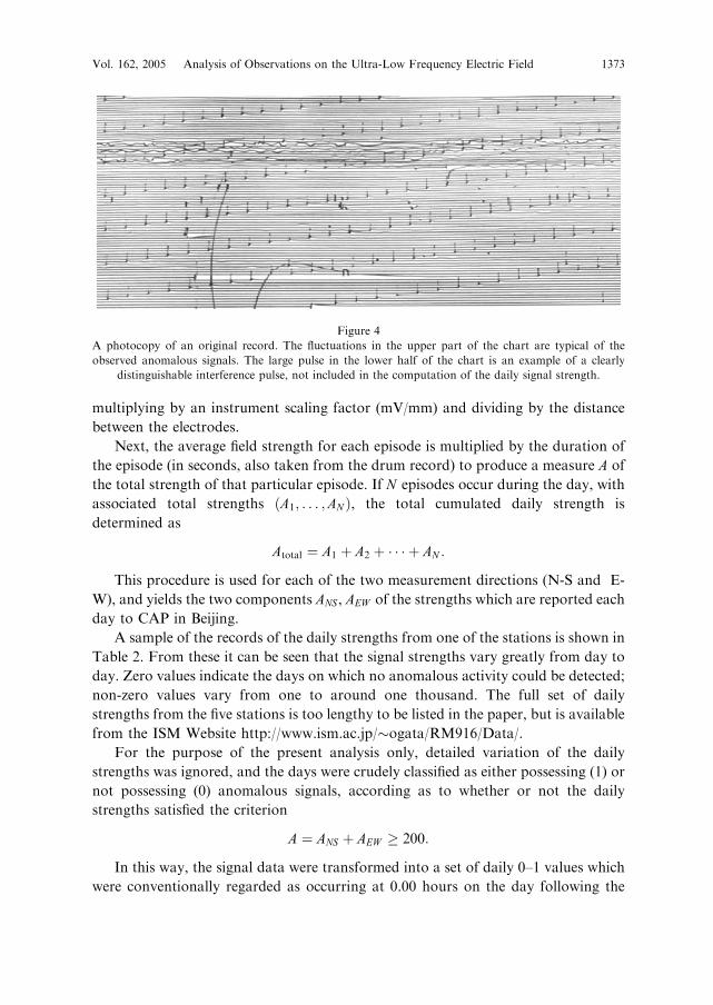
throughout the day, but in episodes. A given episode may assume a variety of forms,

but most commonly appears on the drum record as a signal of roughly sinusoidal

character with irregular amplitude and frequency (see Fig. 4).

The measure adopted to quantify the daily signal strength is a rough estimate of

the total cumulative amplitude (duration times mean amplitude), computed as

described below.

First, for each episode in each of the two measurement directions (N-S and E-W),

an average amplitude is estimated from the drum record by taking half the maximum

throw on the chart plus half an approximate mean-square value. The average

amplitude of the episode is then converted to an average electric field strength by

Table 1

Observation periods and observed numbers of events at each station

Station Location Observation period NEQ NEQ=T NES NES=NEQ

Huailai 40�260; 115�310 ’87-05-1 � ’98-01-31 59 5.32 239 4.05

Langfang 39�320; 116�410 ’82-01-1 � ’96-12-31 77 5.13 366 5.73

Sanhe 39�590; 117�040 ’82-01-1 � ’98-01-31 75 5.00 266 3.55

Changli 39�480; 119�190 ’90-01-1 � ’96-12-31 22 3.14 42 6.00

Qingxian 38�350; 116�500 ’82-01-1 � ’96-12-31 60 2.20 271 8.21

NEQ: Number of earthquakes; NES : Number of electric signal events. Rates are in events/year.

1372 J. Zhuang et al. Pure appl. geophys.,

multiplying by an instrument scaling factor (mV/mm) and dividing by the distance

between the electrodes.

Next, the average field strength for each episode is multiplied by the duration of

the episode (in seconds, also taken from the drum record) to produce a measure A of

the total strength of that particular episode. If N episodes occur during the day, with

associated total strengths ðA1; . . . ;AN Þ, the total cumulated daily strength is

determined as

Atotal ¼ A1 þ A2 þ � � � þ AN :

This procedure is used for each of the two measurement directions (N-S and E-

W), and yields the two components ANS , AEW of the strengths which are reported each

day to CAP in Beijing.

A sample of the records of the daily strengths from one of the stations is shown in

Table 2. From these it can be seen that the signal strengths vary greatly from day to

day. Zero values indicate the days on which no anomalous activity could be detected;

non-zero values vary from one to around one thousand. The full set of daily

strengths from the five stations is too lengthy to be listed in the paper, but is available

from the ISM Website http://www.ism.ac.jp/�ogata/RM916/Data/.

For the purpose of the present analysis only, detailed variation of the daily

strengths was ignored, and the days were crudely classified as either possessing (1) or

not possessing (0) anomalous signals, according as to whether or not the daily

strengths satisfied the criterion

A ¼ ANS þ AEW � 200:

In this way, the signal data were transformed into a set of daily 0–1 values which

were conventionally regarded as occurring at 0.00 hours on the day following the

Figure 4

A photocopy of an original record. The fluctuations in the upper part of the chart are typical of the

observed anomalous signals. The large pulse in the lower half of the chart is an example of a clearly

distinguishable interference pulse, not included in the computation of the daily signal strength.

Vol. 162, 2005 Analysis of Observations on the Ultra-Low Frequency Electric Field 1373

signal readings. This series was then used as one of the components in the later

correlation studies. Table 1 lists for each station the number of days on which

earthquake events were recorded, the number of days on which signal events (1’s)

were recorded, and the ratio between these numbers. The last column is included as a

possible indicator of the noisiness of the site, in terms of the number of electric signal

days not directly associated with earthquakes. The occurrences are displayed in

Figure 5, together with the earthquake data for each station.

3.2 Recognition of Interference Signals

Experience has shown that low-sky or sky-to-ground lightning, power lines that

leak electricity to the ground near the station, and local domestic or industrial

activities may influence electric field observations made using the buried electrode

method. Some sources of noise can be distinguished easily from the anomalous

signals described earlier by the differences in character of the recorded waveforms. As

an example, Figure 6 shows both waveforms typical of the anomalous signals, and a

single large pulse typical of an interference signal. Figure 6 shows the interference

signals from low-sky lightning and power line leakages near the station.

Table 2

A segment of the records of daily strength from the Sanhe station

Date ANS AEW ANS þAEW

1982-04-23 0 0 0

1982-04-24 0 0 0

1982-04-25 0 0 0

1982-04-26 0 0 0

1982-04-27 0 0 0

1982-04-28 434 134 568

1982-04-29 217 19 236

1982-04-30 389 167 556

1982-05-01 401 211 612

1982-05-02 216 17 233

1982-05-03 50 0 50

1982-05-04 389 122 511

1982-05-05 322 17 339

1982-05-06 611 235 846

1982-05-07 16 1 17

1982-05-08 37 2 39

1982-05-09 0 0 0

1982-05-10 12 1 13

1982-05-11 0 0 0

1982-05-12 2 0 2

1982-05-13 1 0 1

1982-05-14 0 0 0

For the purposes of the present analysis, electric signals are noted as having been present on a given day if

and only if the total strength ANS þ AEW exceeds 200. In other cases the signals are noted as having been

absent.

1374 J. Zhuang et al. Pure appl. geophys.,

When clearly distinguishable features of the latter kind are observed, they are

excluded from the calculation of the daily strengths. In all other cases, irrespective of

their supposed source, fluctuations above the noise level are assumed to form part of

the anomalous signal, and are included in the calculation of the daily strengths.

3.3 Earthquake Data

For each station, a special subcatalogue was prepared, consisting of events for

which either

(a) the epicentral distance from the station was less than 200 km, and the local

magnitude was 4.0 or greater, or

34

56

34

56

34

56

34

56

1982 1984 1986 1988 1990 1992 1994 1996 1998

Time (Year)

Mag

nitu

de

Huailai

Langfang

Sanhe

Changli

Qingxian

34

56

(a)

(b)

(c)

(d)

(e)

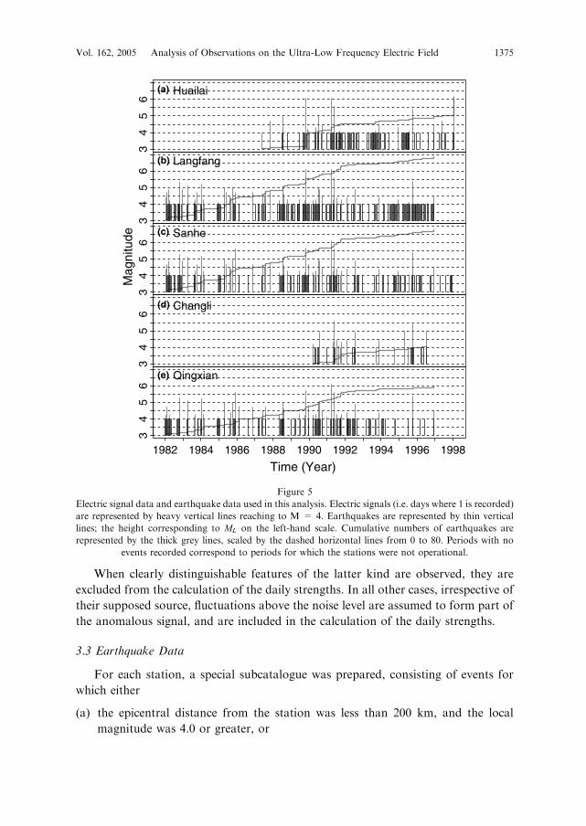
Figure 5

Electric signal data and earthquake data used in this analysis. Electric signals (i.e. days where 1 is recorded)

are represented by heavy vertical lines reaching to M = 4. Earthquakes are represented by thin vertical

lines; the height corresponding to ML on the left-hand scale. Cumulative numbers of earthquakes are

represented by the thick grey lines, scaled by the dashed horizontal lines from 0 to 80. Periods with no

events recorded correspond to periods for which the stations were not operational.

Vol. 162, 2005 Analysis of Observations on the Ultra-Low Frequency Electric Field 1375

(b) the epicentral distance from the station was less than 300 km, and the local

magnitude was 5.0 or greater.

The data for these subcatalogues were extracted from the main China catalogue

prepared by CAP; copies of this catalogue, if required for research purposes, can be

obtained from the weblink http://www-wdcds.seis.ac.cn (contact Professor Ma Li in

case of difficulties, as the Website is currently in Chinese only).

An epicentral plot of earthquakes with local magnitudes 4 and greater occurring

within an approximately 800-km square region around Beijing is shown in Figure 1.

Earthquakes falling into at least one of the five subcatalogues are shown with dark

circles; other earthquakes are shown with light circles. Time-magnitude plots of the

earthquakes from the subcatalogues for each of the five selected stations are shown in

Figure 5.

The five subcatalogues are also condensed and summarized in Table 3. The table

lists origin times, epicenters and local magnitudes for each event, and indicates the

stations for which the given event fell within one or the other of the two specified

circles. For each station, the earthquake events satisfying the prescribed criteria were

coded as a sequence of occurrence times, ignoring magnitudes and other coordinates.

The two series for each station, one series for the electric signals and the other for the

earthquakes, formed the inputs for the analyses described below.

None of the subcatalogues has been declustered prior to the analysis; rather, the

clustering effect is itself modelled through the self-exciting term in the models

discussed in the next section. Indeed, a secondary aim of the paper is to check the

extent to which clustering can affect the apparent significance of the electric signals

Figure 6

A photocopy of a record with noises (the upper panel) from ground strong lightning and (the bottom

panel) from electricity leaked by power lines. In the upper panel the short vertical bars, which form up a

line intersecting the horizontal line, are the timing marks at every minute, and irregular pulses caused by

strong ground lightning are marked by arrows. In the bottom panel, the part in black represents the period

of power leakage.

1376 J. Zhuang et al. Pure appl. geophys.,

Table 3

List of the earthquakes in this analysis. The coding in the last column indicates the stations for which the given

event lay within one or the other of the observation circles: H = Huailai, L = Langfang, S = Sanhe,

C = Changli, Q = Qingxian. Lower suffix (e.g., H1) refers to a smaller event within 200 km radius. Upper

suffix (1) refers to a larger event in outer annulus (M > 5 between 200 and 300 km from station). Double

suffix (11) refers to a larger event within the smaller circle

Date Time Latitude Longitude Magnitude Remark

1982-01-20 14:54:13 37�020 117�320 4.2 Q1

1982-01-26 17:47:57 37�240 114�520 4.8 Q1

1982-01-27 12:30:42 39�450 118�460 4.4 S1C1

1982-02-09 17:33:37 39�380 118�090 4.7 L1S1C1

1982-03-08 03:41:59 39�520 118�400 4.9 S1C1

1982-03-30 12:06:33 39�480 118�300 4.2 S1C1

1982-07-09 17:18:24 38�070 119�230 4.1 C1

1982-08-09 04:07:11 38�580 120�350 4.0 C1

1982-10-19 20:46:01 39�530 118�590 5.3 L1S1C11

1982-12-10 02:16:46 40�280 116�330 4.9 H1L1S1

1983-01-31 01:50:03 37�260 115�010 4.1 L1Q1

1983-02-06 08:05:47 37�310 114�570 4.5 L1Q1

1983-04-03 10:16:30 40�450 114�470 5.1 H11L

1

1983-07-21 05:55:55 40�490 114�420 4.4 H1

1983-08-03 14:21:15 37�380 119�060 4.4 C1

1983-08-08 09:04:58 40�400 115�230 4.1 H1L1

1983-08-21 05:00:31 39�430 118�190 4.1 S1C1

1983-08-26 17:22:18 39�480 117�130 4.3 H1L1S1C1

1983-09-09 22:12:45 40�280 116�340 4.0 H1L1S1

1983-09-15 12:18:35 37�310 114�160 4.1 Q1

1983-10-05 00:25:17 39�510 118�540 4.7 S1C1

1984-01-07 19:18:22 39�430 118�450 5.2 L1S1C11

1984-02-27 05:00:08 39�260 118�010 4.3 L1S1C1

1984-03-11 11:24:07 39�380 118�220 4.0 S1C1

1984-03-16 11:43:54 38�280 119�050 4.0 S1C1

1984-05-17 11:08:26 38�580 119�080 4.2 S1C1

1984-11-27 09:54:20 40�300 114�080 4.5 H1

1984-11-27 09:58:20 40�290 114�160 4.1 H1

1984-12-13 11:20:25 39�390 118�130 4.1 S1C1

1985-01-26 20:55:53 37�220 114�460 4.2 Q1

1985-04-22 11:31:33 39�450 118�460 5.0 L1S1C11

1985-04-22 19:02:37 39�440 118�470 4.3 S1C1

1985-04-22 19:56:59 39�430 118�460 4.7 S1C1

1985-05-22 18:51:44 39�500 118�320 4.7 S1C1

1985-08-11 01:17:16 39�440 118�450 4.0 S1C1

1985-08-11 01:30:32 39�450 118�470 4.5 S1C1

1985-08-11 02:29:15 39�460 118�460 4.0 S1C1

1985-08-23 23:19:31 39�450 118�450 4.0 S1C1

1985-08-25 17:05:19 39�440 118�300 4.4 S1C1

1985-10-05 12:01:58 39�470 118�270 5.0 H1L1S11C

11Q

1

1985-10-17 00:08:25 39�170 114�390 4.1 H1L1Q1

1985-11-21 19:42:22 40�050 115�500 4.7 H1L1S1

1985-11-23 08:47:14 38�470 121�110 4.5 C1

1985-11-30 22:38:00 37�140 114�490 5.6 L1S1Q11

1986-01-11 17:54:35 37�260 114�540 4.1 L1Q1

Vol. 162, 2005 Analysis of Observations on the Ultra-Low Frequency Electric Field 1377

Table 3

(Continued )

Date Time Latitude Longitude Magnitude Remark

1986-02-05 17:18:36 39�450 118�260 4.0 S1C1

1986-02-15 07:08:47 37�450 115�140 4.8 L1Q1

1986-02-18 06:07:03 37�480 115�110 4.5 L1Q1

1986-07-02 11:56:58 38�230 120�290 4.6 C1

1986-07-02 11:58:29 38�240 120�300 4.3 C1

1986-11-10 16:58:05 40�030 116�430 4.7 H1L1S1

1986-12-16 07:25:56 37�160 114�450 4.2 Q1

1987-03-21 07:00:23 38�170 114�150 4.5 L1Q1

1987-05-22 11:50:42 40�000 116�470 4.0 H1L1S1

1987-06-07 12:26:23 39�320 118�050 4.5 L1S1C1

1987-07-16 02:16:28 39�470 118�380 4.5 S1C1

1987-08-08 07:35:06 39�200 117�530 4.7 L1S1C1

1987-08-08 17:35:08 39�200 117�540 4.1 L1S1C1

1987-11-11 21:18:39 40�170 114�480 4.7 H1L1

1988-05-09 06:22:01 39�180 118�060 4.2 L1S1C1

1988-07-23 13:51:43 40�050 114�130 5.0 H11L

11S

1Q1

1988-07-25 01:47:39 39�310 118�060 4.4 L1S1C1

1988-07-26 22:46:39 39�340 118�060 4.9 L1S1C1

1988-07-30 18:44:32 39�460 118�430 4.3 S1C1

1988-08-03 17:44:11 39�360 118�390 4.6 S1C1

1988-10-26 01:29:44 39�520 118�290 4.3 S1C1

1989-06-18 14:50:59 39�400 118�190 4.3 S1C1

1989-07-23 03:15:09 37�220 115�020 4.3 Q1

1989-10-05 11:55:35 39�370 118�150 4.2 S1C1

1989-10-18 22:57:23 39�570 113�500 5.7 H11L

1S1Q1

1989-10-18 23:29:59 39�570 113�500 4.2 H1

1989-10-19 00:52:55 39�570 113�480 4.2 H1

1989-10-19 01:01:34 39�570 113�490 6.1 H11L

1S1Q1

1989-10-19 01:09:43 39�540 113�460 4.0 H1

1989-10-19 01:11:17 39�580 113�490 5.1 H11L

1S1Q1

1989-10-19 01:26:26 40�000 113�510 4.4 H1

1989-10-19 02:20:46 39�590 113�520 5.6 H11L

1S1Q1

1989-10-19 05:02:03 39�550 113�490 4.4 H1

1989-10-19 18:29:03 39�550 113�440 5.1 H11L

1S1Q1

1989-10-20 01:56:48 39�560 113�480 4.1 H1

1989-10-20 19:41:41 39�590 113�540 4.1 H1

1989-10-23 21:19:32 39�550 113�490 5.2 H11L

1S1Q1

1989-10-29 10:22:43 39�560 113�490 4.1 H1

1989-12-09 07:04:51 39�530 113�490 4.2 H1

1989-12-13 09:10:11 39�560 113�530 4.1 H1

1989-12-14 12:13:01 37�360 115�170 4.8 L1Q1

1989-12-25 04:26:23 40�200 118�570 4.7 C1

1989-12-31 16:24:48 39�580 113�510 4.0 H1

1990-03-16 15:08:39 39�460 118�270 4.2 S1C1

1990-05-23 14:13:01 40�130 116�280 4.3 H1L1S1

1990-07-21 08:41:51 40�350 115�500 5.0 H11L

11S

1Q1

1990-07-23 16:41:32 39�450 118�290 4.9 S1C1

1990-08-03 18:05:44 37�530 115�020 4.2 L1Q1

1990-09-22 11:02:19 40�050 116�220 4.5 H1L1S1

1378 J. Zhuang et al. Pure appl. geophys.,

Table 3

(Continued)

Date Time Latitude Longitude Magnitude Remark

1990-12-24 13:31:03 37�540 115�010 4.1 L1Q1

1991-01-29 06:28:04 38�280 112�320 5.5 H1

1991-03-26 02:02:38 39�580 113�510 6.1 H11L

1S1Q1

1991-03-26 02:07:27 39�590 113�500 4.3 H1

1991-04-01 05:35:23 39�540 113�490 4.0 H1

1991-05-07 00:25:01 39�480 118�420 4.3 S1C1

1991-05-29 19:02:10 39�430 118�180 5.2 H1L1S11C

11Q

1

1991-05-30 07:06:55 39�410 118�160 5.6 H1L1S11C

11Q

1

1991-07-11 19:05:05 39�410 118�230 4.3 S1C1

1991-07-27 17:54:47 39�510 118�480 4.4 S1C1

1991-08-21 05:28:28 37�200 114�420 4.3 Q1

1991-08-22 06:23:37 37�280 114�440 4.1 Q1

1991-09-02 04:17:42 38�490 119�590 4.1 C1

1991-09-20 17:52:06 39�200 114�050 4.1 H1L1

1991-09-28 08:37:47 40�050 117�030 4.0 H1L1S1

1991-09-28 18:48:06 40�040 117�040 4.0 H1L1S1

1991-10-05 05:44:39 39�180 117�570 4.0 L1S1C1

1991-10-07 07:25:21 37�560 115�040 4.1 L1Q1

1991-10-17 02:19:42 39�440 118�250 4.3 S1C1

1992-02-14 17:08:43 39�460 118�260 4.4 S1C1

1992-07-22 05:43:02 39�170 117�560 4.9 L1S1C1

1993-06-14 03:01:00 37�250 119�560 4.1 C1

1993-08-30 07:27:59 39�540 113�490 4.1 H1

1993-08-30 08:13:38 39�540 113�490 4.0 H1

1993-09-27 15:44:16 39�390 118�420 4.0 S1C1

1993-11-18 07:05:09 39�360 117�270 4.4 L1S1C1

1994-10-04 15:54:17 39�440 118�260 4.0 S1C1

1994-12-23 13:13:40 40�280 115�330 4.3 H1L1

1995-06-27 09:39:51 38�140 119�280 4.0 C1

1995-07-20 20:51:23 40�160 115�260 4.1 H1L1S1

1995-10-06 06:26:53 39�400 118�200 5.4 H1L1S11C

11Q

1

1995-11-13 14:33:19 39�220 113�120 4.5 H1

1996-04-08 00:39:28 39�510 118�440 4.0 S1C1

1996-12-16 05:36:33 40�100 116�300 4.5 H1L1S1

1996-12-16 09:52:24 40�060 116�350 4.0 H1L1S1

1997-04-12 15:05:02 38�170 120�290 4.3 C1

1997-05-25 14:59:08 40�420 114�520 4.7 H1

1998-01-10 11:50:39 41�060 114�180 6.2 H11L

1

1998-01-10 11:59:17 41�200 114�320 4.0 H1

1998-01-10 12:09:58 41�060 114�280 4.5 H1

1998-01-10 13:03:59 41�050 114�300 4.6 H1

1998-01-10 15:38:18 41�090 114�320 4.2 H1

1998-01-10 20:01:55 41�070 114�260 4.0 H1

1998-01-10 21:50:32 41�110 114�260 4.3 H1

1998-01-10 23:33:20 41�040 114�250 4.0 H1

1998-01-11 02:37:47 41�050 114�250 4.6 H1

1998-01-11 11:31:43 41�050 114�260 4.4 H1

1998-01-12 02:41:54 41�080 114�270 4.3 H1

1998-01-12 18:32:29 41�120 114�280 4.3 H1

Vol. 162, 2005 Analysis of Observations on the Ultra-Low Frequency Electric Field 1379

terms (cf. MICHAEL, 1997). With the exception of Huailai station, for which the 300

km observation region includes the aftershock regions of both the Datong and

Zhangbei events, the number of direct aftershocks entering the subcatalogues is

rather small, as can be verified from Figure 5.

3.4 Some Features of the Data

From the preceding tables and plots, several important features can be seen which

may be useful to bear in mind for the subsequent analysis.

1. Much of the earthquake activity during the study period is associated with three

major earthquake groups. The first represents continuing low-level activity in an

extended region around the epicenter of the 1976 MS ¼ 7:8 Tangshan earthquake.

This activity continued into the early 1990s. The other two major groups are

mainly aftershocks of the two M ¼ 6:4 Datong earthquakes of 1991/1992, and of

the 1998 M ¼ 6:2 Zhangbei earthquake. The entire region was quiet between these

two events.

2. The clustering effect is particularly pronounced for the Huailai station, the study

region for which encompassed both the Datong and Zhangbei clusters, as well as

partially extending into the region of the Tangshan events. By contrast, the

Changli station entered the study only in 1990, and lies too far to the East to

contain the smaller (4 � M < 5) aftershocks from either the Datong or the

Zhangbei sequences. Its subcatalogue shows the least clustering of all five stations.

Table 3

(Continued)

Date Time Latitude Longitude Magnitude Remark

1998-01-14 01:17:26 41�040 114�270 4.2 H1

1998-01-14 11:09:57 41�110 114�310 4.3 H1

1998-01-17 10:41:18 41�060 114�260 4.3 H1

1998-01-18 04:07:25 41�090 114�220 4.6 H1

1998-01-18 06:17:54 41�070 114�280 4.3 H1

1998-01-22 12:11:51 41�080 114�260 4.4 H1

1998-01-27 07:29:07 41�020 114�290 4.2 H1

1998-02-13 07:05:05 41�030 114�270 4.0 H1

1998-04-14 10:47:48 39�410 118�280 5.0 H1L1S11C

11Q

1

1998-04-14 10:48:06 39�410 118�280 4.4 S1C1

1998-04-16 07:13:44 41�050 114�270 4.0 H1

1998-06-02 09:32:04 41�110 114�240 4.8 H1

1998-06-02 10:47:29 41�030 114�300 4.5 H1

1998-07-14 18:16:08 41�060 114�270 4.4 H1

1998-07-27 09:05:16 41�120 114�290 4.8 H1

1998-07-27 09:16:56 41�060 114�270 5.0 H11L

1

1998-07-27 11:17:48 41�100 114�290 4.7 H1

1998-08-13 18:21:52 41�010 114�350 4.7 H1

1998-08-15 18:11:22 38�380 119�140 4.4 S1C1

1380 J. Zhuang et al. Pure appl. geophys.,

3. The electric signals are also very highly clustered, even on some occasions when

there appear to be no associated earthquakes. This feature is particularly

pronounced for Langfang and Huailai stations, both of which show substantially

increased electric signals activity in the later part of the record. These two stations,

especially Langfang, were affected by urbanization of their immediate environ-

ment during the study period. Urbanization has not occurred to the same extent at

the other stations. The increased activity observed at the first two stations may

therefore give some indication of the sort of interference effects to be expected

from man-made sources.

4. Self-exciting and Mutually Exciting Models

In this section we describe the model used for the major part of the analysis. The

self-exciting and mutually exciting earthquake model was developed by Ogata and

Utsu (see OGATA et al., 1982; OGATA, 1983; UTSU and OGATA, 1997) from the

Hawkes process (HAWKES, 1971). It is most easily described through its conditional

intensity function,

kðtÞdt ¼ E½NðdtÞjHt�; ð1Þ

whereHt ¼ fObservation history up to time tg. In essence, the conditional intensity

function represents the target process as a time-varying Poisson process with rate kðtÞconditioned by past history. The conditional intensity function of the combined self-

exciting and mutually-exciting model (referred to as the combined model in the rest

of the paper) can be written as

kðtÞ ¼ lþ kSðtÞ þ kEðtÞ; ð2Þ

where l represents the constant background rate, kS is the self-exciting term, which

models clustering among the target events, and kE is the external excitation term,

which models the contribution to the rate from the external process. The self-exciting

term is taken in the form

kSðtÞ ¼X

ti<t

gðt � tiÞ; ð3Þ

with the summation extended to all the events occurring before time t in the target

process fti : i ¼ 1; 2; . . . ; n1g, gðtÞ being a sum of Laguerre polynomials

gðtÞ ¼ e�atXNS

k¼0pktk: ð4Þ

Similarly, the external excitation term is written as

kEðtÞ ¼X

ui<t

hðt � uiÞ; ð5Þ

Vol. 162, 2005 Analysis of Observations on the Ultra-Low Frequency Electric Field 1381

with the summation taken over all the events occurring before time t in the process of

precursor events (here the electric signals) fui : i ¼ 1; 2; . . . ; n2g, hðtÞ again being a

sum of Laguerre polynomials,

hðtÞ ¼ e�btXNE

k¼0qktk: ð6Þ

The Laguerre polynomials are used here as a convenient family of orthogonal

functions which in principle can be used to model the response functions to any

required degree of accuracy; more detailed discussions of the model are given in

VERE-JONES and OZAKI (1982), OGATA et al. (1982), MA and VERE-JONES (1997), or

the IASPEI manual, UTSU and OGATA (1997). The model was used in the earlier

studies mainly to investigate possible triggering effects between different kinds of

seismicity.

In practice, the number of terms included in the sum has to be balanced between

concerns of sensitivity and overfitting, and is the main target of the model-selection

procedures described later.With limited data, as in the present situation, and little prior

knowledge as to the likely form of the response functions, the fitted response functions

can be interpreted only as crude approximations to any underlying physical processes.

Usually, the excitation effect in the fitted model reaches its maximum immediately

or shortly after an event occurs, then decays quickly with time and becomes

negligible after sufficient time.

If we drop out kE, the model becomes a self-exciting model; if we drop out kS , the

model becomes an externally excited model; if both kS and kE are neglected, the

model reduces to a Poisson model. All of these types of models will be used in our

analysis.

We shall keep the notation fti : i ¼ 1; 2; . . . ; n1g for the main or target process,

and fui : i ¼ 1; 2; . . . ; n2g for the external exciting process or secondary process.

In our analysis, we first take the earthquake events as the target process and the

anomalous electric signals as the external process, to ascertain whether the electric

signals have explanatory power in relation to the occurrence times of earthquakes.

Then we reverse the roles of the two processes, take the anomaly events as the main

process and earthquakes as the external process, to see whether the electric signals

might be triggered by some mechanism following the occurrence of an earthquake.

Given a set of observation data, the parameters of the model can be estimated by

maximizing the likelihood function, which for a conditional intensity model has the

standard form (analagous to that for a Poisson process)

log LðhÞ ¼X

i:0�ti�T

log kðti; hÞ �Z T

0

kðt; hÞdu; ð7Þ

1382 J. Zhuang et al. Pure appl. geophys.,

where ti denotes the occurrence time of the ith event, ½0; T � is the observation time

interval, and H is the vector of parameters (see, for example, DALEY and VERE-

JONES, 2002, Chapter 7).

The parameters for the combined model can be written as

h ¼ ðl; a; p1; p2; . . . ; pNS ; b; q1; q2; . . . ; qNEÞ:

Model selection, particularly the determination of the numbers of parameters NS and

NE in the Laguerre expansions, was carried out using the Akaike Information

Criterion (AIC, see Akaike, 1974). The statistic

AIC ¼ �2maxh

log LðhÞ þ 2kp ð8Þ

is computed for each of the models fitted to the data, where kp is the total number of

fitted parameters. In comparing models with different numbers of parameters,

addition of the quantity 2kp roughly compensates for the additional flexibility which

the extra parameters provide. The model with the lowest AIC value is taken as giving

the optimal choice for forward prediction purposes.

Insofar as it depends on the likelihood ratio, the AIC can also be used as a rough

guide to model testing. As a rule of thumb, in testing a model with k þ d parameters

against a null model with just k parameters, we take a difference of 2 in AIC values as

a rough estimate of significance at the 5% level. If standard asymptotics were

applied, such a difference would correspond to a significance level of 4.6% when

d ¼ 1, 5% when d ¼ 2; 4:6% when d ¼ 3, and 3.5% when d ¼ 5. Such figures give a

rough guide to significance levels, although should be used conservatively, because of

the relatively small sample sizes and other approximations.

One of the main advantages of the combined model in the present context is that

it allows the effect of the electric signals terms to be examined even in the presence of

clustering (modelled by self-excitation) in the earthquakes themselves.

5. Main Analysis

In the main analysis, we use the model format available within the Lin-Lin

program (UTSU and OGATA, 1997). This requires all coefficients in the trend and

polynomial expansions to be nonnegative, thus ensuring positivity of the conditional

intensity, at the expense of flexibility in the functional forms available.

The combined model is fitted separately to data from the five selected stations in

the Beijing region, namely Huailai, Changli, Sanhe, Qingxian and Langfang. Because

of data availability, the observation time intervals for those stations are different, as

summarized in Table 1.

Taking the earthquakes as the target events, we consider the following models to

examine the relationship between the electric signals and the earthquakes:

Vol. 162, 2005 Analysis of Observations on the Ultra-Low Frequency Electric Field 1383

1. Poisson process with polynomial trend (restricted to second order);

2. self-exciting model, without external excitation;

3. externally excited model without self-excitation;

4. combined model of both self-exciting and external excitation terms.

In Section 6, to test whether the electric signal might be a postseismic effect, we

interchange the roles of the electric signals and the earthquakes.

5.1 Self-exciting versus Poisson Models

The purpose of this step is to determine the size and significance of the clustering

effect among the earthquakes before using the self-exciting model as a base model to

determine the contribution of the electric signals in fitting the earthquake data. This

step was accomplished by fitting the self-exciting model to the earthquake data, and

comparing it to the Poisson model with polynomial trend. The first and second row

Table 4

Results from fitting models to the earthquake data

Station NP NS NE kp logL AIC �kp logL=L0 �AIC

Trend model –

Huailai 2 – – 2 )33.66 71.31 – – –

Langfang 1 – – 1 )50.77 103.54 – – –

Sanhe 1 – – 1 )56.67 115.34 – – –

Changli 1 – – 1 )25.29 52.58 – – –

Qingxian 1 – – 1 )54.52 111.06 – – –

Self-exciting model vs. Trend model

Huailai 1 1 – 3 89.10 )170.22 1 122.76 241.53

Langfang 1 1 – 3 )22.77 51.55 2 28.00 )51.99Sanhe 1 1 – 3 )39.98 83.96 2 16.69 )31.38Changli 1 1 – 3 )23.11 52.22 2 2.18 )0.36Qingxian 1 1 – 3 )42.23 90.47 2 12.28 )20.59

Externally excited model vs. Trend model

Huailai 1 – 2 4 15.68 )23.35 2 49.34 )94.66Langfang 1 – 2 4 )30.14 68.28 3 20.63 )35.26Sanhe 1 – 2 4 )32.20 72.46 3 34.47 )42.88Changli 1 – 1 3 )20.13 46.26 2 5.16 )6.32Qingxian 1 – 2 4 )26.08 60.17 3 28.44 )50.99

Combined model vs. Self-exciting model

Huailai 1 1 2 6 100.86 )189.72 3 11.76 )19.50Langfang 1 1 2 6 )8.70 29.40 3 14.07 )22.15Sanhe 1 1 2 6 )15.83 43.66 3 24.15 )40.30Changli 1 1 1 5 )17.67 45.34 2 5.44 )6.88Qingxian 1 1 2 6 )22.65 57.31 3 19.58 )33.16

NS : order of the Laguerre polynomial used for the self-exciting term; NE: order of the Laguerre polynomial

used for the external excitation term; kp: total number of fitted parameters in the model; logL: maximized

log likelihood; AIC: as defined by (8); Dp: difference between the numbers of parameters in the two models

for comparison; logL=L0: log-likelihood ratio of the two models for comparison; DAIC: difference in AIC

between the two models for comparison.

1384 J. Zhuang et al. Pure appl. geophys.,

blocks in Table 4 list the outputs from this analysis for each of the five selected

stations.

From this table we can see that the clustering effect plays an important role in the

process of the earthquake occurrences. For each station except Changli the reduction

in AIC is very substantial, well above what would be required to establish

significance at around the 5% level. The effect is particularly pronounced for Huailai,

as we might expect from the clusters contained within the Huailai record. The

changes in seismicity rate for Huailai were mainly caused by these clusters, therefore

here and elsewhere we have restricted the trend to a second degree polynomial with

nonnegative coefficients. The Changli station, by contrast, shows a relatively small

degree of clustering, large enough for the self-exciting model to be preferred to the

Poisson model, although barely large enought to establish the significance of the

clustering effect.

We conclude that clustering should be taken into account for all five stations, and

that it is a particularly important feature for the stations closest to the source regions

of the Datong and Zhangbei clusters.

5.2 Externally Excited versus Poisson Models

We next compare the Poisson model to the externally excited models for the five

data sets (see the third row block in Table 4). We see that the electric signals reduce

the Poisson AIC values by amounts which are less than the reductions due to the self-

exciting terms for Huailai and Langfang stations, but comparable to or greater than

those reductions for Sanhe, Changli and Qingxian stations. These large differences

suggest that the external signals have considerable explanatory power. However, we

shall see that these values are somewhat inflated, being based in part on the fact that

both earthquakes and signals are clustered, so that to a degree the electric signals can

act as a surrogate for the self-exciting terms.

5.3 Combined versus Self-exciting Models

Finally, we compare the fits of the self-exciting and combined models. The final

row block of Table 4 shows that the addition of the external excitation terms to the

self-exciting terms contributes further reductions of the AIC values for all five

stations. All five reductions are substantial, even though smaller than those obtained

by testing the electric signals models directly against the Poisson model. Note that the

differences in AIC values between the combined model and the Poisson model are

very much larger than the differences between the externally excited model and the

Poisson. Both effects demonstrate that the explanatory power of the electric signals is

considerably exaggerated unless the clustering terms are taken into account, as

forewarned by MICHAEL (1997). The important conclusion, however, is that the

electric signals retain a significant explanatory power even after the clustering has

been taken into account by the self-exciting terms.

Vol. 162, 2005 Analysis of Observations on the Ultra-Low Frequency Electric Field 1385

Additional insight can be obtained by examining the information gains per event.

This quantity — here just the difference in log-likelihoods normalized by the number

of events — is a measure of the improvement in predictability in passing from the

base model to the test model (see e.g., VERE-JONES (1998) or HARTE and VERE-JONES

(2005) for further discussion; the idea revisits early papers by Kagan (e.g., KAGAN

and KNOPOFF, 1977). The gains per earthquake event for each station are shown in

Table 5, together with the gains per signal event in passing from the self-exciting to

the combined model. It is interesting that the stations showing the smallest degree of

clustering show the largest gains/event. The low gains per electric signal for Huailai

and Langfang suggest that these stations may be more subject to interference from

noisy signals than the other stations, although the low gains may also represent just a

further nuisance effect of the clustering.

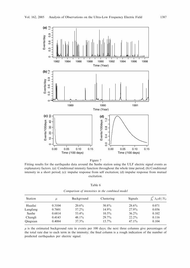
5.4 Fitted Conditional Intensity and Impulse Response Functions

An example of the conditional intensity function of the combined model, and the

associated impulse response functions, is shown in Figure 7 for the Sanhe station.

The response functions are only crudely fitted because of the rather small amount of

earthquake data. The shapes of the impulse response functions gðtÞ and hðtÞ suggestthat the relative risk of earthquakes is high during the first few days after the

occurrence of an earthquake or an electric signal event, then decays rapidly with

time. Note, however, the differences in scales for the self-exciting and electric signals

terms. The latter is much more diffuse, although the apparent rate of decay for both

response functions may be exaggerated by the choice of Laguerre functions,

associated with exponential decay, as the function basis (see further discussion in

Section 6). The differences between the maximum absolute values of two functions

gðtÞ and hðtÞ are an indication that, for this station at least, the immediate increase in

risk due to the occurrence of an earthquake is larger than the immediate increase in

risk from an electric signal event.

Table 5

Information gains per earthquake and per signal for each station

Station Infogain/earthquake Infogain/earthquake Infogain/signal

(cluster vs Poisson) (combined vs cluster) (combined vs cluster)

Huailai 2.08 0.20 0.049

Langfang 0.36 0.18 0.038

Sanhe 0.22 0.28 0.091

Changli 0.10 0.25 0.130

Qingxian 0.20 0.33 0.072

The information gain means here the log-likelihood ratio, normalized by dividing by the number of

earthquake events or the number of signal events.

1386 J. Zhuang et al. Pure appl. geophys.,

Time (Year)

(a)

Eve

nts/

day

00.

30.

60.

91.

2

1982 1984 1986 1988 1990 1992 1994 1996 1998

Time (Year)

(b)

Eve

nts/

day

00.

30.

60.

91.

2

1989 1990 1991

0.00 0.05 0.10 0.15

010

2030

4050

Time (/100 days)

(c)

Eve

nts/

100d

ays

0.00 0.05 0.10 0.15

0.0

0.4

0.8

1.2

Time (/100 days)

(d)

Eve

nts/

100d

ays

Figure 7

Fitting results for the earthquake data around the Sanhe station using the ULF electric signal events as

explanatory factors. (a): Conditional intensity function throughout the whole time period; (b) Conditional

intensity in a short period; (c): impulse response from self excitation; (d) impulse response from mutual

excitation.

Table 6

Comparison of intensities in the combined model

Station � Background Clustering SignalsR T

0 �Edt=NS

Huailai 0.3104 20.6% 50.8% 28.6% 0.071

Langfang 0.7601 57.2% 14.9% 27.9% 0.056

Sanhe 0.6814 53.4% 10.5% 36.2% 0.102

Changli 0.4143 48.1% 29.7% 22.2% 0.116

Qingxian 0.4084 37.3% 15.7% 47.1% 0.104

l is the estimated background rate in events per 100 days; the next three columns give percentages of

the total rate due to each term in the intensity; the final column is a rough indication of the number of

predicted earthquakes per electric signal.

Vol. 162, 2005 Analysis of Observations on the Ultra-Low Frequency Electric Field 1387

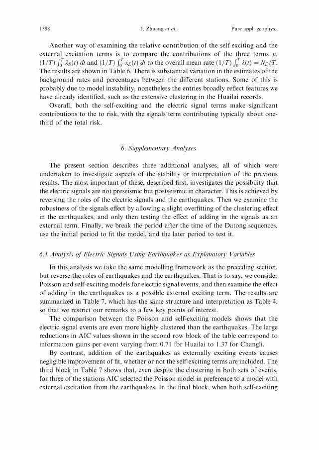
Another way of examining the relative contribution of the self-exciting and the

external excitation terms is to compare the contributions of the three terms l,ð1=T Þ

R T0 kSðtÞ dt and ð1=T Þ

R T0 kEðtÞ dt to the overall mean rate ð1=T Þ

R T0 kðtÞ ¼ NE=T .

The results are shown in Table 6. There is substantial variation in the estimates of the

background rates and percentages between the different stations. Some of this is

probably due to model instability, nonetheless the entries broadly reflect features we

have already identified, such as the extensive clustering in the Huailai records.

Overall, both the self-exciting and the electric signal terms make significant

contributions to the to risk, with the signals term contributing typically about one-

third of the total risk.

6. Supplementary Analyses

The present section describes three additional analyses, all of which were

undertaken to investigate aspects of the stability or interpretation of the previous

results. The most important of these, described first, investigates the possibility that

the electric signals are not preseismic but postseismic in character. This is achieved by

reversing the roles of the electric signals and the earthquakes. Then we examine the

robustness of the signals effect by allowing a slight overfitting of the clustering effect

in the earthquakes, and only then testing the effect of adding in the signals as an

external term. Finally, we break the period after the time of the Datong sequences,

use the initial period to fit the model, and the later period to test it.

6.1 Analysis of Electric Signals Using Earthquakes as Explanatory Variables

In this analysis we take the same modelling framework as the preceding section,

but reverse the roles of earthquakes and the earthquakes. That is to say, we consider

Poisson and self-exciting models for electric signal events, and then examine the effect

of adding in the earthquakes as a possible external exciting term. The results are

summarized in Table 7, which has the same structure and interpretation as Table 4,

so that we restrict our remarks to a few key points of interest.

The comparison between the Poisson and self-exciting models shows that the

electric signal events are even more highly clustered than the earthquakes. The large

reductions in AIC values shown in the second row block of the table correspond to

information gains per event varying from 0.71 for Huailai to 1.37 for Changli.

By contrast, addition of the earthquakes as externally exciting events causes

negligible improvement of fit, whether or not the self-exciting terms are included. The

third block in Table 7 shows that, even despite the clustering in both sets of events,

for three of the stations AIC selected the Poisson model in preference to a model with

external excitation from the earthquakes. In the final block, when both self-exciting

1388 J. Zhuang et al. Pure appl. geophys.,

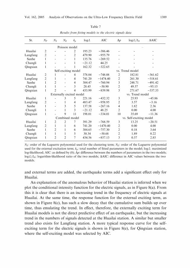
and external terms are added, the earthquake terms add a significant effect only for

Huailai.

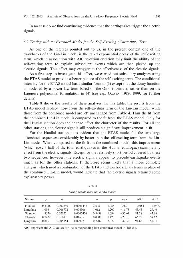
An explanation of the anomalous behavior of Huailai station is inferred when we

plot the conditional intensity function for the electric signals, as in Figure 8(a). From

this it is clear that there is an increasing trend in the frequency of electric signals at

Huailai. At the same time, the response function for the external exciting term, as

shown in Figure 8(c), has such a slow decay that the cumulative sum builds up over

time, thus emulating the trend. In effect, therefore, the externally exciting term for

Huailai models is not the direct predictive effect of an earthquake, but the increasing

trend in the numbers of signals detected at the Huailai station. A similar but smaller

trend also exists for Langfang station. A more typical response curve for the self-

exciting term for the electric signals is shown in Figure 8(e), for Qingxian station,

where the self-exciting model was selected by AIC.

Table 7

Results from fitting models to the electric signals data

St. NP NS NE kp logL AIC Dp logL=L0 DAIC

Poisson model –

Huailai 2 - - 2 195.23 )386.46 - - -

Langfang 2 - - 2 479.90 )955.79 - - -

Sanhe 1 - - 1 135.76 )269.52 - - -

Changli 1 - - 1 )21.12 44.25 - - -

Qingxian 1 - - 1 162.32 )322.65 - - -

Self-exciting model vs. Trend model

Huailai 2 1 - 4 378.04 )748.08 2 182.81 )361.62Langfang 2 1 - 4 741.20 )1474.40 2 261.30 )518.61Sanhe 1 2 - 4 384.47 )760.94 3 248.71 )491.42Changli 1 1 - 3 28.45 )50.90 2 49.57 )95.15Qingxian 1 2 - 4 433.99 )859.98 3 271.67 )537.33

Externally excited model vs. Trend model

Huailai 1 - 3 5 221.16 )432.32 3 25.93 )45.86Langfang 2 - 1 4 483.47 )958.95 2 3.57 )3.16Sanhe 1 - 3 5 137.58 )267.16 4 1.82 2.36

Changli 1 - 1 3 )21.12 48.25 2 0.00 4.00

Qingxian 1 - 9 11 198.01 )334.01 10 35.69 )11.36Combined model vs. Self-exciting model

Huailai 1 2 2 7 391.29 )768.59 3 13.25 )20.51Langfang 2 1 1 6 741.20 )1470.40 2 0.00 4.00

Sanhe 1 2 1 6 384.65 )757.30 2 0.18 3.64

Changli 1 1 1 5 30.34 )50.68 2 1.89 0.22

Qingxian 1 2 2 7 434.56 )857.13 3 0.57 2.85

NS : order of the Laguerre polynomial used for the clustering term; NE : order of the Laguerre polynomial

used for the external excitation term; kp: total number of fitted parameters in the model; logL: maximized

log-likelihood; AIC: as defined by (8); Dp: difference between the numbers of parameters in the two models;

logL=L0: logarithm-likelihood ratio of the two models; DAIC: difference in AIC values between the two

models.

Vol. 162, 2005 Analysis of Observations on the Ultra-Low Frequency Electric Field 1389

Time (Year)

Eve

nts/

day

00.

30.

71

1.3

1.7

1987 1989 1991 1993 1995 1997

(a)

0.00 0.05 0.10 0.15

05

1015

Time (/100 days)

Eve

nts/

100d

ays

(b)

0 10 20 30 40 50

0.00

0.04

0.08

0.12

Time (/100 days)E

vent

s/10

0day

s

(c)

Time (Year)

Eve

nts/

day

(d)

00.

10.

30.

5

1982 1984 1986 1988 1990 1992 1994 1996

0.00 0.05 0.10 0.15

05

1015

Time (/100 days)

Eve

nts/

100d

ays

(e)

Figure 8

Fitting results for the ULF electric signal events from the Huailai and Qiangxian stations using the

earthquake data as explanatory factors. (a) Conditional intensity function at Huailai station; (b) impulse

response from self excitation at Huailai station; (c) impulse response from external excitation at Huailai

station; (d) conditional intensity function at Qingxian station; (e) impulse response from self-excitation at

Qingxian station (no response from external excitation because the model with only self-exciting terms is

selected).

1390 J. Zhuang et al. Pure appl. geophys.,

In no case do we find convincing evidence that the earthquakes trigger the electric

signals.

6.2 Testing with an Extended Model for the Self-Exciting (Clustering) Term

As one of the referees pointed out to us, in the present context one of the

drawbacks of the Lin-Lin model is the rapid exponential decay of the self-exciting

term, which in association with AIC selection criterion may limit the ability of the

self-exciting term to explain subsequent events which are then picked up the

electric signals. This effect may exaggerate the effectiveness of the electric signals.

As a first step to investigate this effect, we carried out subsidiary analyses using

the ETAS model to provide a better picture of the self-exciting term. The conditional

intensity for the ETAS model has a similar form to (3) except that the decay function

is modelled by a power-law term based on the Omori formula, rather than on the

Laguerre polynomial formulation in (4) (see e.g., OGATA, 1989, 1999, for further

details).

Table 8 shows the results of these analyses. In this table, the results from the

ETAS model replace those from the self-exciting term of the Lin-Lin model, while

those from the combined model are left unchanged from Table 4. Thus the fit from

the combined Lin-Lin model is compared to the fit from the ETAS model. Only for

the Huailai station does the change affect the character of the results. For all the

other stations, the electric signals still produce a significant improvement in fit.

For the Huailai station, it is evident that the ETAS model fits the two large

aftershock sequences considerably by better than the self-exciting term from the Lin-

Lin model. When compared to the fit from the combined model, this improvement

(which covers half of the total earthquakes in the Huailai catalogue) swamps any

effect from the electric signals. Except for the relatively short period covered by these

two sequences, however, the electric signals appear to precede earthquake events

much as for the other stations. It therefore seems likely that a more complete

analysis, which used a combination of the ETAS and electric signals terms in place of

the combined Lin-Lin model, would indicate that the electric signals retained some

explanatory power.

Table 8

Fitting results from the ETAS model

Station � K c � p logL AIC AICl

Huailai 0.3346 0.002340 0.0001442 2.608 1.088 120.2 )230.4 )189.72Langfang 1.008 0.006772 0.004906 1.012 1.200 )16.73 43.45 29.40

Shanhe .8576 0.02022 0.0007426 0.3438 1.094 )35.64 81.28 43.66

Changli 0.7429 0.01807 0.01675 0.0000 1.423 )28.10 66.20 59.62

Qingxian 0.8161 0.005854 0.02902 0.2707 2.029 )42.32 94.63 57.31

AICl represent the AIC-values for the corresponding best combined model in Table 4.

Vol. 162, 2005 Analysis of Observations on the Ultra-Low Frequency Electric Field 1391

6.3 Testing with Separate Learning and Evaluation Periods

In Table 9, we summarize the results of fitting the Lin-Lin and ETAS models to

data from the Sanhe station (the one with the longest record) in two parts. The first

(training) period, 1982 to end 1989 was used to fit the Poisson, self-exciting,

combined, and ETAS models; the second (evaluation) period (1990 to end 1998) was

used to assess the performance of the model on an independent data set. The

combined model produced the lowest AIC during the training period, and was clearly

selected as the best of the four models. The combined model also yielded the highest

log-likelihood value in the evaluation period. More than 1/3 of the earthquakes in the

Sanhe catalogue (26) occurred during the evaluation period, making the information

gain/earthquake (comparing combined to self-exciting, as in Table 5) about

7:5=26 � 0:28, which is quite comparable to the overall gains reported in that table.

The results for the Huailai station again reveal the dominance of the clustering term

as registered by the ETAS model. When compared to the self-exciting model, there is

still a modest information gain/event.

7. Discussion and Conclusions

In this paper we have used a version of the Hawkes mutually-exciting model to

examine the statistical correlations between the electric signal events, which were

recorded by five stations in the Beijing region, and the intermediate-size earthquakes

which occurred within a 200–300 km radius of each of the stations. For each station

Table 9

Training and evaluation

Sanhe

Training (NEQ ¼ 49) Prediction (NEQ ¼ 26)

1982.1.1 – 1989.12.31 1990.1.1 – 1998.1.31

Model logL AIC logL

Combined 0.87 10.26 )23.67Self-exciting )11.07 28.15 )31.20

ETAS )8.99 27.98 )29.08Poisson )23.67 49.34 )36.01

Huailai

Training (NEQ ¼ 23) Prediction(NEQ ¼ 36)

1982.1.1 – 1990.12.31 1991.1.1 – 1998.1.31

Model logL AIC logL

Combined 43.18 )74.35 48.18

Self-exciting 38.16 )70.32 48.54

ETAS 56.90 )103.80 60.37

Poisson )10.59 23.18 )24.95

1392 J. Zhuang et al. Pure appl. geophys.,

separately, the results indicate that the signals provide weak but nonetheless

nontrivial precursory information regarding the occurrence of magnitude 4 and

larger earthquakes in the circular region around the station. In the converse direction

the results are equally unequivocal; in no case do the earthquakes appear to carry

significant precursory information pertaining to the occurrence of the signal events

recorded at the station.

In response to concerns expressed by the referees and others who have

commented on earlier drafts of this paper, we would like to make the following

comments.

1. While it may be that the electric signals data analyzed in this study have been

collected by relatively simple equipment, and that the initial data handling

requires a degree of subjective intervention and interpretation, the data analyzed

are part of a systematic, standardized process of measurement and reporting that

has been carried out in the Beijing region for the better part of twenty years. From

the point where they have been collected by CAP, the data used are quantitative,

objective, and available for analysis. Within CAP, they form a regular and

integral part of the surveillance and forecasting program, and have done so for

many years.

2. During the period of the study, all five stations report very comparable effects,

despite local variations in seismicity and geological and man-made environment.

Even if the observation period is sectioned, similar effects are observed in each

section, as outlined in Section 6.3. The principal deviations from the common

pattern occur for the Huailai station. Even here it seems likely that the

discrepancies are caused by the two large aftershock sequences which enter the

earthquake subcatalogue for this station, and that the discrepancies would be

extensively reduced if the aftershock periods were either better modelled in the

combined model, or removed from the analysis.

3. The statistical analysis applied to these data is also crude. Information is lost in

converting the signals to 0–1 data, and only the simple Lin-Lin model has been

used in the main analysis. Nevertheless it is sufficient to show that the precursory

effect of the electrical signals persists even after allowance has been made for

earthquake clustering, and that the electric signals are pre- and not postseismic in

character. Interpretation of the AIC values and associated significance levels is

subject to uncertainty, however in most cases there is a large margin of error. The

fact that similar significance levels are recorded for all stations substantially

increases the overall significance.

4. It is clear that in some cases the signals have been contaminated by the occurrence

of electric storms, man-made electrical appliances, etc. Except in the most obvious

cases, all such disturbances have been incorporated into the assessment of the

daily strengths. In such a situation, unless the interfering signals carried predictive

information similar to those of the anomalous signals themselves, one would

Vol. 162, 2005 Analysis of Observations on the Ultra-Low Frequency Electric Field 1393

expect them to act as noise and to decrease the apparent correlations between the

signals and earthquakes. Additional studies by Guan and coworkers suggest that

in fact the majority of the observed signals are not related to interference from

meteorological phenomena or magnetic storms. For example, the electric signals

do not appear to reflect annual fluctuations in rainfall or temperature (GUAN et

al., 1996), nor do the large-scale magnetic storms appear to be associated with

major variations in either the electric signals or the earthquakes (ibid). As for

man-made signals, the two sites most likely to be affected by these, namely

Langfang and Huailai, both show increased frequency of electric signals with

time, and are accompanied by rather low values of the predictive power per signal.

These features suggest that, for these stations at least, the earthquake-associated

signals are indeed diluted by noise signals which build-up as urbanization of the

area increases. At least for the observation periods in the present study, however,

these effects are not so large as to destroy the correlations with the earthquakes.

5. At present, we have no answer to what may be the most serious problem

associated with the present topic, namely the absence of a plausible physical

process that can explain the source and precursory character of the electric

signals. Our view here is that the existence of such a mechanism cannot yet be

ruled out, and that in such a situation the collection and presentation of empirical

data, such as outlined in the present study, is a necessary stage in the scientific

process.

6. Although we are aware of the controversy which has surrounded earlier reports of

links between ground electric signals and earthquake occurrence, and the many

serious criticisms which have been directed towards some of these, we believe that

the present data and analysis should be given the opportunity to be considered in

their own right. At the least the data analyzed here summarize the results of two

decades of preparatory work which is unique of its kind in scale and consistency

of application.

In conclusion, we should emphasize that this is only a preliminary analysis of the

data on electric signals held by the China Seismological Bureau Centre of Analysis

and Prediction. Its aim was to establish that there is at least a prima facie case for

taking seriously the claims that there may be a connection between electric signals

and earthquakes. At this point, we cannot fully exclude the possibility that the

positive results obtained in this analysis have their roots in aspects of the data

handling, selection procedures, and analysis, or in some coincidental relation

between earthquake occurrence and man-made or physical noise. Our belief,

however, is that this is unlikely to be the case.

We should also emphasize that the present paper does not pretend to set up a

quantitative forecasting scheme. It is based on a retrospective study of existing data,

and leaves unresolved many issues relating to the combination of information from

the different stations, and the estimation of locations and sizes of possible future

1394 J. Zhuang et al. Pure appl. geophys.,

earthquakes, all of which would have to be resolved before a quantitative forecasting

scheme could be put into place. Some of these aspects are pursued further in the

companion study by ZHUANG et al. (2002), which is currently available as a technical

report; its partial findings are summarized in OGATA and ZHUANG (2001).

Currently, the electric signals stations around Beijing are in the process of being

converted to digital stations. When this process is completed, it should allow an

unequivocal answer to be given to concerns about reliability and objectivity of the

data which have been raised. Should the results confirm the findings in the present

report, the existing data will be a unique source of information about the electric

signals, and their protection becomes a matter of both national and international

importance.

Acknowledgements

We would like to acknowledge the critical but nonetheless helpful advice that we

have received from the Referees (Yan Kagan and Francesco Mulargia), from Robert

Davies, and from other colleagues, all of whom have contributed substantially to

improvements to the original draft of this paper. The work described in the present

study was initialized with assistance of No. 10371012 of the National Natural Science

Foundation of China, then was supported primarily with partial assistance of a

subcontract on earthquake forecasting with the Institute of Geological and Nuclear

Sciences on FRST Contract Natural Hazards of New Zealand and Gran-in-Aid

(B)(2)14380128 for Scientific Research from theMinistry of Education, Science, Sport

and Culture, Japan. The observation part on the ground ULF electric signals by the

fourth author has been supported byNo. 2001BA601B01-05-03 of the 10th Five-Year-

Term Scientific Research Funds of China Seismological Bureau. J. Zhuang is also

supported by a post-doctoral program P04039 founded by Japan Society for the

Promotion of Science. All of this financial assistance is gratefully acknowledged here.

Thewriting of the paperwas assisted by grants from theCenter forMathematics and its

Applications in Minneapolis.

REFERENCES

AKAIKE, H. (1974), A New Look at the Statistical Model Identification, IEEE Trans. Automatic Control,

AC-19, 716–723.

CHEN, Z., DU, X., SONG, R., and GUAN, H., Electromagnetic Radiation and Earthquakes (in Chinese),

(Seismological Press, Beijing, 1998).

CHEN, Z. and XU, C., Features of electric-magnetic radiation between some shallow earthquakes in North

China. In Studies on New Method of Short-term Earthquake Prediction (eds. Department of Monitoring,

State Seismology Bureau), (Seismological Press, Beijing, 1994), 57–63.

DALEY, D. and VERE-JONES, D., An Introduction to the Theory of Point Processes, vol. 1. (2nd edition)

(Springer, New York, 2002).

GUAN, H. and LIU, G. (1995), Electromagnetic Radiation Anomalies Before Moderate and Strong

Earthquakes, Acta Seismologica Sinica 9, 289–299.

Vol. 162, 2005 Analysis of Observations on the Ultra-Low Frequency Electric Field 1395

GUAN, H., CHEN, Z., and YU, S. (1996) Analysis on the Relationship Between Earthquakes and Electric-

magnetic Radiation, Earthquake Research in China 16, 168–176.

GUAN, H., ZHANG, H., LIU, Y., YU, S., and CHEN, Z. (1999), Studies on the Relationship Between the

Anomalies of the Ultra-Low Frequency Electric Field and Earthquakes (in Chinese with English abstract),

Earthquake 19, 142–148.

GUAN, H., CHEN, Z., and YU, S. (2000), Study on Seismic Precursor Features of Electromagnetic Radiation

in the Beijing Region and its Surrounding Area (In Chinese with English abstract), Earthquake 20, 65–70.

HARTE, D. and VERE-JONES, D. (2005), The entropy score and its Uses in Earthquake Forecasting, Pure

Appl. Geophys. 162, 1229–1253.

HAWKES, A. G. (1971), Spectra of Some Self-exciting and Mutually Exciting Point Processes, Biometrika

58, 83–90.

KAGAN, Y. Y. and KNOPOFF, L. (1977), Earthquake Risk Prediction as a Stochastic Process, Phys. Earth

and Planet. Inter., 14, 97–108.

MA, L. and VERE-JONES, D. (1997), Application of M 8 and Lin-Lin Algorithms to New Zealand Earthquake

Data, New Zealand J. Geol. Geophys., 35, 77–89.

MICHAEL, A. (1997), Test Prediction Methods: Earthquake Clustering Versus the Poisson Model, Geophys.

Res. Lett., 24, 1891–1894.

OGATA, Y., AKAIKE, H., and KATSURA, K. (1982), The Application of Linear Intensity Models to the

Investigation of Causal Relations Between a Point Process and Another Stochastic Process, Ann. Inst.

Statist. Math. 34, 373–387.

OGATA, Y. (1983), Likelihood Analysis of Point Processes and its Application to Seismological Data, Bull.

Internat. Statist. Inst. 50, 943–961.

OGATA, Y. (1989), Statistical Model for Standard Seismicity and Detection of Anomalies by Residual

Analysis for Point Process, Tectonophysics 169, 1–16.

OGATA, Y. (1999), Seismicity Analysis Through Point-process Modelling: A Review, Pure Appl. Geophys.

155, 471–507.

OGATA, Y. and ZHUANG, J. (2001), Statistical examination of anomalies for the precursor to earthquakes,

and the multi-element prediction formula: Hazard rate changes of strong earthquakes M � 4:0 around

Beijing area based on the ultra-low frequency electric observation (1982–1997), Report of the

Coordinating Committee for Earthquake Prediction, Geographical Survey Institute, Tsukuba, Japan,

66, 562–570.

UTSU, T. and OGATA, Y. (1997), Statistical analysis of seismicity. In Algorithm for Earthquake Statistics

and Prediction, IAPSPEI Software Library (International Association of Seismolog and Physics of the

Earth’s Interior 6, 13—94).

VERE-JONES, D. and OZAKI, T. (1982), Some Examples of Statistical Estimation Applied to Earthquake

Data, Ann. Inst. Statist. Math. 34, 189–207.

VERE-JONES, D. (1998), Probabilities and Information Gain for Earthquake Forecasting, Computat. Seismol.

30, 248–263.

ZHUANG, J., OGATA, Y., VERE-JONES, D., MA, L., and GUAN, H. (2002), Statistical confirmation of a

relationship between excitation of the utra-low frequency electric signals and magnitude M � 4 earthquakes

in a 300 km radius region around Beijing, Research Memorandum 847, Institute of Statistical

Mathematics, Tokyo, Japan.

(Received September 15, 2003, accepted April 30, 2004)

To access this journal online:

http://www.birkhauser.ch

1396 J. Zhuang et al. Pure appl. geophys.,