1 2 3 4 5 6 7 8 9 1011121314151617181920212223242526272829303132333435363738394041424344454647484950515253545556575859606162636465

Design of steel beams with discrete lateral restraintsFinian McCanna,*, Leroy Gardnera and M. Ahmer Wadeea

email: finian.mccann07@imperial.ac.uk; leroy.gardner@imperial.ac.uk; a.wadee@imperial.ac.uk

aDepartment of Civil and Environmental Engineering, Imperial College London, London SW7 2AZ,

United Kingdom

*Corresponding author. Tel: +44 7517 477765

Abstract

Discrete lateral restraints offer an effective means of stabilizing beams against lateral-

torsional buckling. Design expressions for simply-supported beams braced regularly along

their span with elastic restraints, based on analytically-derived formulae, are presented herein.

These include the minimum restraint stiffness required to force the beam to buckle in between

the restraint nodes and the forces induced in the restraints, along with a brief treatment of

the critical moment of the beam. It is demonstrated that there is close agreement between the

values obtained from the design formulae and their original analytical counterparts. These are

also compared with the results from design formulae based on analogous column behaviour,

an approach commonly used in design codes. It is found that the column rules used by design

codes return values that, when compared with the results of the current analysis, are overly

conservative for cases where the restraints are positioned at the compression flange of the

beam but unsafe for restraints positioned at the shear centre.

Keywords: steel beams; discrete lateral restraints; beam stability; steel beam design

1

TitleClick here to view linked References

1 2 3 4 5 6 7 8 9 1011121314151617181920212223242526272829303132333435363738394041424344454647484950515253545556575859606162636465

1 Introduction

Slender beams are susceptible to failure through lateral-torsional buckling, an instability phe-nomenon involving both lateral deflection and twist of the cross-section of the beam. The classicalresult for the critical lateral-torsional buckling moment of an unrestrained simply-supported beamunder constant bending moment, as given by [1], is:

Mob =π2EIzL2

√IwIz

+L2GItπ2EIw

. (1)

where the material properties E and G are the Young’s modulus and elastic shear modulus,respectively, of steel; the cross-sectional properties Iz, Iw and It are the minor-axis second momentof area, the warping stiffness and the St. Venant’s torsional constant, respectively.

The stability of a beam can be enhanced through the provision of bracing members that restraineither one, or both, of these forms of displacement, thus increasing the overall load that the beamcan safely support. Restraints can be continuous, like profiled metal sheeting, or discrete, like roofpurlins. If they inhibit the amount of twist then they are described as torsional braces; if theyinhibit lateral deflection, they are described as lateral braces. The current work focusses on beamswith discrete lateral braces.

The British Standard BS 5950 [2] states that a cross-section can be assumed to be restrainedlaterally if the intermediate restraint at that section is sufficiently stiff to inhibit any lateraldeflection of the compression flange relative to the supports. Moreover, BS 5950 states that,for one or two restraints, the members should be able to withstand a total force of 2.5% of themaximum compressive force in the beam, divided amongst the restraints in proportion to theirspacing; for three or more restraints, each restraint should be able to withstand 1% of the maximumcompressive force (or the 2.5% force distributed in proportion to the restraint spacing). Meetingthese requirements allows the designer to divide the beam into segments with pin-joints assumedto exist at the bracing points. These segments are then checked individually to ensure stabilitythroughout the beam.

The American Institute of Steel Construction Specifications for Structural Steel Buildings [3]primarily requires that lateral bracing members are to be attached at the compression flange ofthe beam (or to both flanges if the beam is in double curvature); the scope of the current workexteneurocodeds to braces located at an arbitrary height relative to the shear centre of the beam.The finite element analysis of [4] showed the negative effect of web distortion on the efficacyof lateral restraints, and so it is assumed in the current work that adequate web-stiffening isprovided at bracing nodes. The cross-section of the beam at these points may hence be assumedto be rigid and that Vlasov conditions prevail. With regard to the strength of the braces, the AISCspecifications require that they must be able to withstand an equivalent of 2% of the maximumcompressive force in the beam for beams in single curvature (4% for restraints beside an inflectionpoint for beams in positive and negative curvature in the same span). The minimum stiffnessrequirement for nodal bracing, using the notation of the current work, is:

K =1

0.75

4M

Luhs(2)

where K is the restraint stiffness, M is the maximum moment in the beam, hs is the distancebetween the centroids of the flanges and Lu is the unbraced length of the beam. Interestingly, theformulation suggests that providing additional braces to a particular beam, which would reducethe unbraced length, leads to an increase in brace stiffness requirements.

The Eurocode EN 1993-1-1 [5] is less prescriptive than BS 5950 and the AISC specifications,merely stating that beams with sufficient restraint to the compression flange are not susceptible tolateral-torsional buckling and that the elastic critical moment should take into account (amongstother things) the influence of lateral restraints, thus leaving the designers to decide whether todivide the beam into laterally-unrestrained segments, or to use a method of determining the elasticcritical moment of a laterally-restrained beam. It does not specify one particular restraint force

1

ManuscriptClick here to view linked References

1 2 3 4 5 6 7 8 9 1011121314151617181920212223242526272829303132333435363738394041424344454647484950515253545556575859606162636465

ratio that the bracing members must be able to withstand, but instead, an equivalent stabilizingforce based on the initial imperfection of the beam is determined, and the bracing system as a wholeshould be able to withstand this. For one member restrained, assuming the initial imperfectionto be L/500, this rule equates to a distributed restraint force ratio of at least 1.6%, depending onthe stiffness of the bracing system. The 1.6% value is a lower bound, since it is based upon theassumption that the restraining system does not deflect. Previous work presented in [6], [7] and[8] suggest that a figure closer to 1% is sufficient, and that members with this level of strengthcan be assumed also to possess a level of stiffness adequate to restrain the bracing nodes fully;this assumption, however, does not hold for all geometries and bracing layouts, particularly wherebracing is provided closer to the shear centre of the beam.

Both the British and European design codes fail to provide a method of determining directly thestiffness required of the restraint to ensure that buckling occurs between the restraints, while theAmerican specifications are formulated for restraint provided at the compression flange. Methodsto determine the required stiffness for specific cases are detailed by [9], amongst others. It istherefore the aim of the current work to provide design formulae for beams with an arbitrarynumber of restraints spaced at regular intervals, positioned at an arbitrary height above the shearcentre.

2 Analytical method and results

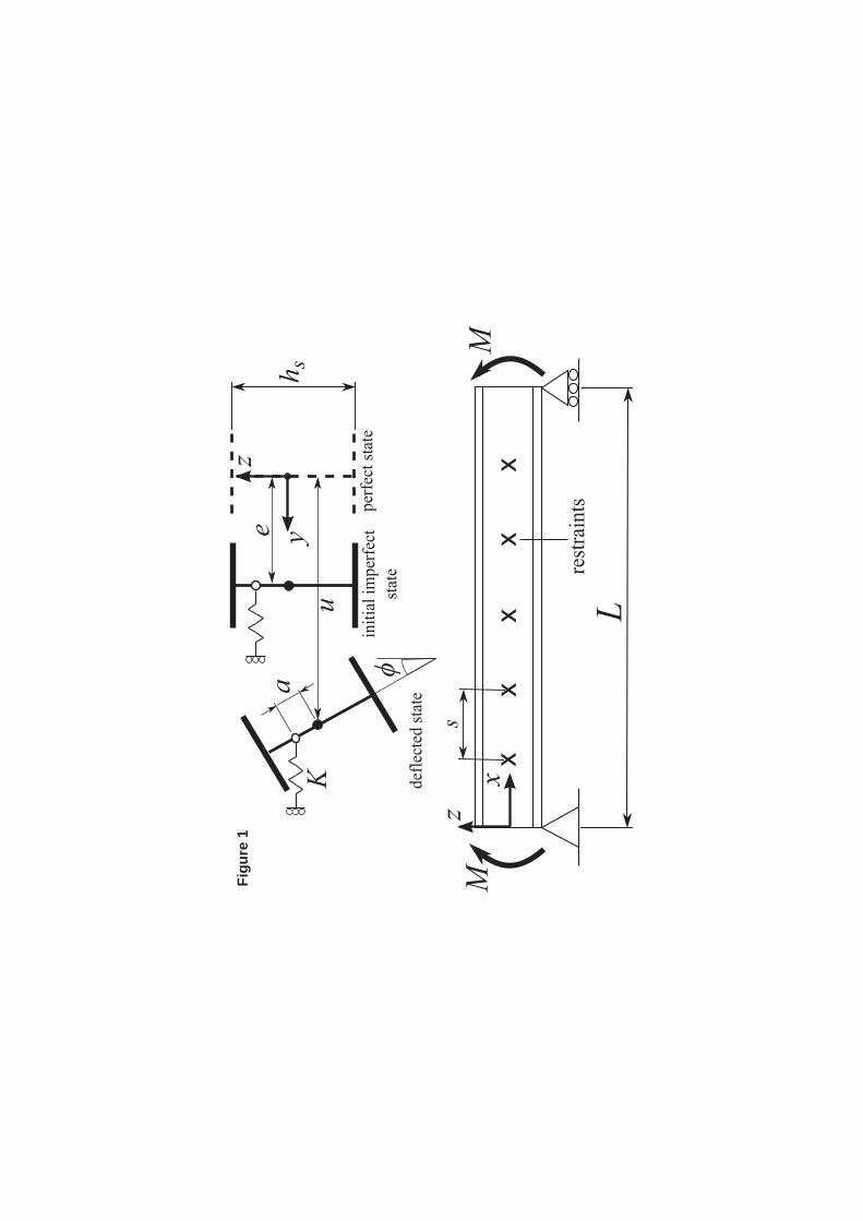
A linear Rayleigh–Ritz analysis is used to determine the critical moment and deflected shape ofa simply-supported doubly-symmetric I-section beam of span L, with a number nb of discreteelastic lateral restraints, of stiffness K, positioned at regular intervals along the span of the beam,such that the restraint spacing s = L/(nb + 1) (see Figure 1). The restraints are all positionedat a height a above the shear centre of the cross-section; positive values of a denote compressionside bracing, while negative values denote tension side bracing. The beam is loaded with major-axis end moments of magnitude M acting in opposite senses. In keeping with classical analysessuch as those of [10] and [1], the system is assumed to have two degrees-of-freedom: the lateraldisplacement of the shear centre, u and the angle of twist of the cross-section, φ; these are modelledas Fourier sine series, with the coefficients of cosine terms set equal to zero to satisfy the boundaryconditions of zero deflection and zero twist at the supports:

u =

∞∑n=1

un sin(nπx

L

), (3)

φ =∞∑

n=1

φn sin(nπx

L

), (4)

where un and φn are the generalized coordinates of the system. The initial lateral imperfection ofthe beam is represented by a single half-sine wave of amplitude e1, i.e. e = e1 sin(πx/L). Since thesystem is linearized by assuming small deflections and modelling the restraints as linear springs,the highest order of terms in un and φn in the potential energy functional of the system, V , istwo.

The deflected shape of the beam is determined by solving the simultaneous equilibrium equa-tions ∂V/∂un = 0 and ∂V/∂φn = 0 for un and φn. From these expressions it is possible tocalculate the forces induced in the restraints.

The critical moment of the beam is determined by solving det(H) = 0 for M , where H is thematrix of the second derivatives of V with respect to the generalized coordinates; these derivativesare equivalent to the coefficients of the second order terms of V because of the linear nature ofthe system. Analysis of the system shows that the possible buckling modes separate into twoclasses: a finite number nb of node-displacing modes and an infinite number of modes where thebeam buckles in between the restraints, which are related to harmonics that are integer multiplesof (nb + 1). A solution for the critical moment for such modes – termed internodal modes – is

2

1 2 3 4 5 6 7 8 9 1011121314151617181920212223242526272829303132333435363738394041424344454647484950515253545556575859606162636465

easily-obtainable; the most critical mode is that of a beam buckling in nb + 1 half-sine waves andso the associated critical moment, MT , is equivalent to the critical moment of an unrestrainedbeam segment of span s:

MT =π2EIzs2

√IwIz

+s2GItπ2EIw

. (5)

This moment is termed the threshold moment. In the case of the node-displacing modes, however,it is not possible to find a closed-form solution for M , but instead an implicit relationship betweenM and the coordinates can be determined [11].

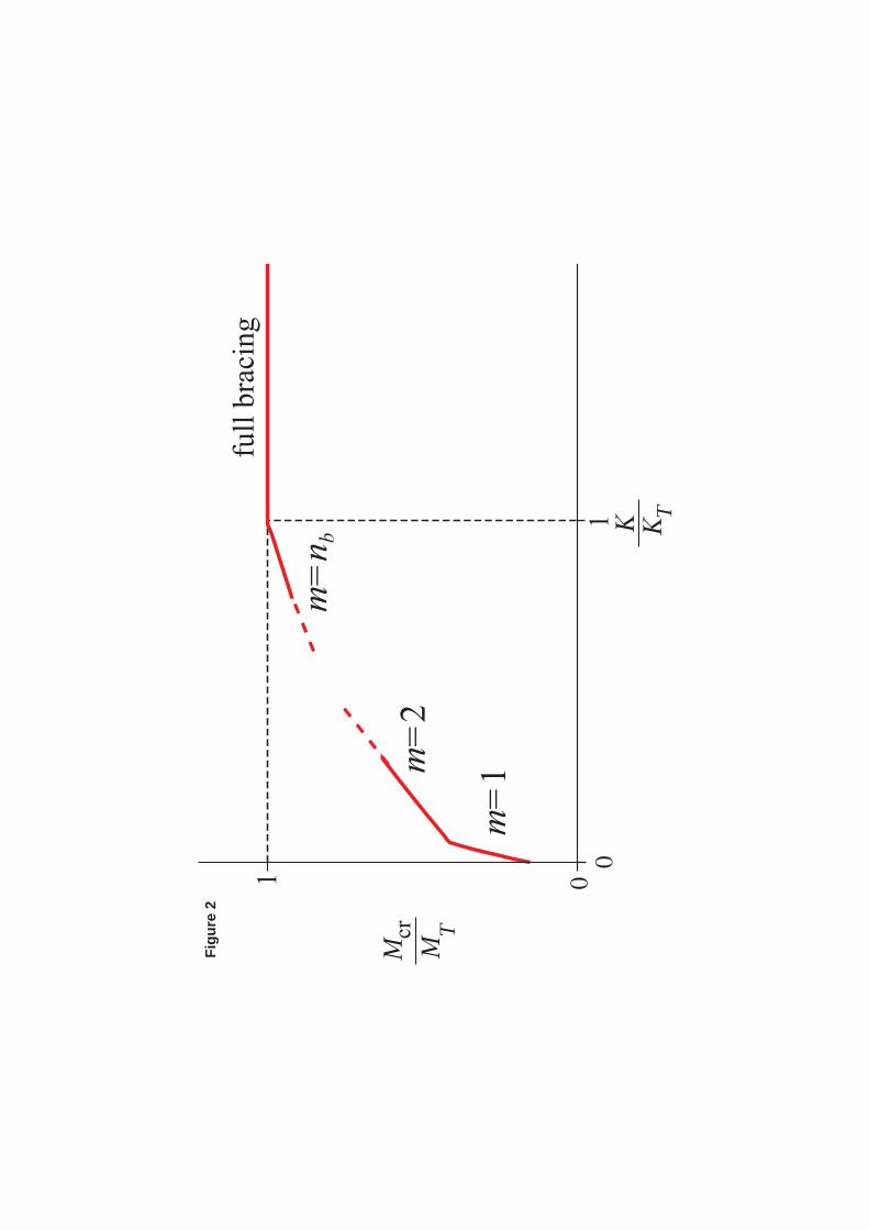
An unrestrained beam, i.e. whereK = 0, buckles into a single half-sine wave. AsK is increased,the critical mode changes, as shown in Figure 2. If the restraints possess adequate stiffness, thebeam buckles in between the restraints, i.e. the internodal buckling mode is critical and hencethe critical moment equals MT . This occurs if the stiffness K exceeds the threshold stiffness KT ;this level of bracing is termed full bracing. If K < KT , then one of the node-displacing modes iscritical. The value of KT for the mth node-displacing mode is determined by substituting MT intothe implicit load–deflection relationship for that mode and determining the conditions necessaryfor an infinite deflection, a condition associated with critical equilibrium in linear systems. It canbe shown [11] that if the restraint height a is greater than a certain limiting value alim then theoverall threshold stiffness of the system is associated with the nbth mode; if restraints are providedbelow this level, it may be assumed that the beam cannot ever develop the fully-braced conditionand hence the concept of a threshold stiffness does not apply. The value of alim is given by:

alim =hsκs

4√1 + κs

, (6)

where κ = L2GIt/π2EIw and κs = κ/(nb + 1)2.

3 Threshold stiffness

Provided the restraints are positioned at a level above alim then the beam has the potential tobe braced fully, the requirement for which being K > KT . The following formula, derived on thebasis of the analytical results, provides an estimate for the threshold stiffness:

KT =

(EIzs3

)62 (1 + κs)

A0 +A1a, (7)

where:A0 = 0.45 + 2.8νb,Tκs, (8)

A1 = 6.3νb,T + 2.2κs − 1, (9)

and the factor νb,T = {1 + cos [π/(nb + 1)]}−1. Values of νb,T for corresponding numbers of

restraints are given in Table 1. Figures 3 to 5 show the close agreement between the analyticaland design formula.

An axially-loaded column with a single restraint located at mid-height buckles into the secondmode if the stiffness of the restraint K > 16π2EIz/L

3; this value represents the equivalent thresh-old stiffness. This varies from being greatly conservative to greatly unsafe across the standardranges of a and κ: for a = 1 the column rule tends to provide estimates that are twice too large;for a = 0, the predicted values range from being 15% too low to nearly 5.5 times too low dependingon the value of κ. Percentage errors are given in Table 2.

4 Critical moment

If K � KT then the elastic critical moment of the beam is the threshold moment, MT :

MT =π2EIzs2

(hs

2

)√1 + κs. (10)

3

1 2 3 4 5 6 7 8 9 1011121314151617181920212223242526272829303132333435363738394041424344454647484950515253545556575859606162636465

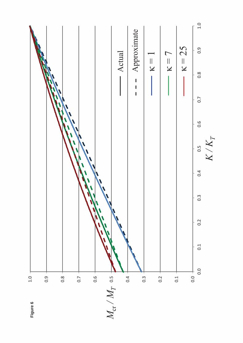
However, if it is the case that K < KT , then the value of Mcr is reduced from this thresholdamount. A conservative estimate for Mcr in such cases is provided by the linear approximation:

Mcr = Mob +K

KT(MT −Mob) . (11)

The above approximation is most accurate for a single restraint at midspan, positioned at thecompression flange, as shown in Figure 6. Accuracy decreases for lower restraint heights and forgreater numbers of restraints. Since there are many freely-available computer packages capableof determining the critical moment of a beam with arbitrary intermediate restraint conditions,further design guidance on the estimation of critical moments is deemed unnecessary. Moreover,it is more often the case that the restraining members are to be designed to brace the beam fully,and so the guidance provided in §3 is of greater use.

The SCI publication P093 [12], which has been updated by SCI publication P360 [13], statedthat a conservative approach to the problem of beam bracing behaviour can be provided bytreating the beam as an analogous column whereby the axial load P is equivalent to the maximumcompressive force in the flanges, = M/hs. For an axially-loaded column braced at midspan by anelastic restraint of stiffness K, the critical load is given by:

Pcr = PE +3

16KL, (12)

up to a limiting stiffness of 16π2EIz/L3, when the beam is fully braced. When compared with

the analytical results of the current work, for top flange bracing, the method returns conservativevalues for all but the smallest beams. However, for lower restraint heights, there exist ranges ofstiffnesses where the method returns conservative estimates for the critical moment and rangeswhere the estimates are unsafe. Hence, it can be said that application of analogous column rulesis not always appropriate in the determination of critical moments.

5 Restraint forces

The design formulae for the restraint force ratio F/P , where F is the force induced in the restraintand P = M/hs is the maximum compressive force in the beam, is obtained by exploiting the formof the analytical result of F/P . The function is rational in K, such that the graph of F/P againstK possesses a single horizontal asymptote, (F/P )∞, termed the “plateau” force, and a singlevertical asymptote, K∞, termed the “spike” stiffness:

F

P= (F/P )∞

(K

K −K∞

). (13)

Since the imperfection is assumed to be a half-sine wave, the restraint force also varies sinusoidallyalong the span of the beam; for convenience, the maximum possible force induced is determined,i.e. the force at midspan. It is initially assumed that the beam is to be designed to support loadlevels close to M = MT , and the design rules outlined in the current section are based upon thisconservative assumption. Methods to account for lower loading levels are treated subsequently.

5.1 Calculation of spike stiffness

Equation (7) is used to calculate K∞, except the factor νb,T is replaced with:

νb,∞ = {1− cos [π/(nb + 1)]}−1. (14)

It is noted that for nb = 1, K∞ = KT . Values of νb,∞ for calculating K∞ are provided in Table3. As is the case for calculating KT , the values of K∞ obtained are more conservative as κ isincreased and also for higher restraint heights, as shown by Figures 7 and 8. Percentage errors aregiven in Table 4.

4

1 2 3 4 5 6 7 8 9 1011121314151617181920212223242526272829303132333435363738394041424344454647484950515253545556575859606162636465

5.2 Calculation of plateau force

Assuming again that M = MT , the design formula is:(F

P

)∞

= 5(e1L

)[σ(nb + 1)

2a+

(1 + κ)σ

5.5 + 4.5nb

]−1

. (15)

For κ < 5(nb − 1), σ = 1; otherwise the following rules can be used to calculate σ for κ � 50 (avalue that greatly exceeds the range of practical UB values):

• For nb = 1, σ = 0.9− 0.01κ (but > 0.7).

• For nb = 2, σ = 0.99− 0.006κ (but > 0.8).

• For nb = 3, σ = 1− 0.004κ (but > 0.85).

• For nb � 4 a conservative value of σ = 0.95 can be taken.

It was advised in [6] that a force of 1% of the axial load in a flange may generally be assumedas the bracing-strength requirement. For restraints positioned close to the compression flange ofa sufficiently high stiffness this is indeed true, but for a combination of low restraint heights andlow values of κ, this is not the case, since F/P can also exceed the 2.5% limit set out by BS 5950,as clearly seen in Figures 9 to 11. As the number of restraints provided gets larger, the effect onF/P is different depending on the restraint height; the ratio reduces for larger restraint heights,but increases for restraints positioned closer to the shear centre. Percentage errors are given inTable 5.

5.3 Modifications for M < MT

In practice, it is desirable to configure the bracing system so that the effects of lateral-torsionalbuckling can be ignored. This condition is termed “fully-restrained” design and occurs whenλLT � λLT,0, where λLT =

√Mc,Rd/Mcr and Mc,Rd is the in-plane bending resistance of the

beam. Both the Eurocode and BS 5950 define λLT,0 = 0.4. If it is assumed that the beam isdesigned to carry a load close to its in-plane bending resistance, i.e. M ≈ Mc,Rd, and that therestraints are stiff enough so that it is fully braced, i.e. Mcr = MT , then M/MT = λ2

LT,0 = 0.16.Thus, in the sake of economy, the design formulae should take values of M < MT into account.

Modification of spike stiffness

A quick but conservative modification can be made by simply scaling K∞,M=MTby M/MT . This

increases in accuracy with increasing nb, especially for low values of κ and nb � 4.However, if greater accuracy is desired then the following modification factor can be applied

to K∞ with only moderately conservative results:

K∞K∞,M=MT

=M −Mob

MT −Mob. (16)

If M < Mob, then K∞ < 0 and for K > 0, 0 < F/P < (F/P )∞, owing to the function F/Ppassing through the origin. Hence, where M < Mob, the value of F/P corresponding to a stiffnessK � KT can be taken as being equal to (F/P )∞, and the actual value of K∞ need not becalculated.

Modification of plateau force

For a = 0, an approximation for (F/P )∞ can be found by simply scaling the value found in§5.2 by M/MT . For a = 1, simply using the value of (F/P )∞,M=MT

provides only slightlyconservative results, with accuracy improving for higher restraint values and low values of κ.If a � 0.15κ/nb, greater economy can be achieved by using a scaling factor of

√M/MT i.e.

(F/P )∞ =√

M/MT (F/P )∞,M=MT.

5

1 2 3 4 5 6 7 8 9 1011121314151617181920212223242526272829303132333435363738394041424344454647484950515253545556575859606162636465

5.4 Comparison with equivalent column rule

In §5.2 it was shown how the blanket rule of a 1% restraint force ratio suggested in [6] for beamswas adequate, if somewhat conservative for restraints positioned closer to the compression flange.For lower restraint heights, this rule and also the BS 5950 rule of 2.5%, which are based oncolumn buckling theory, have been shown to underestimate the actual restraint force ratio by aconsiderable margin. Expressions are provided in [7] and [14] for the restraint force ratio for asimply-supported axially-loaded strut for the cases of a single restraint attached at an arbitrarypoint along the span of the strut, restraints attached at third points and multiple restraints. Forthe case of a single restraint at midspan the following expression is given:

F

P=

e1L

1PE

P − 1

[PE

KL

P

PE+

1

2π

√PE

Ptan

(π

2

√P

PE

)− 1

4

]−1

. (17)

For two restraints, the force F in each restraint is given by:

F

P=

√3

2

e1L

1PE

P − 1

⎡⎣ PE

KL

P

PE+

sin(

π3

√PPE

)π√

PPE

[2 cos

(π3

√PPE

)− 1] − 1

3

⎤⎦−1

. (18)

Corresponding equations for (F/P )∞ are obtained by setting PE/KL = 0 in the denominator.Given a particular nondimensional restraint height a, it is possible to find at what value of κ thevalue of (F/P )∞, as calculated by the column rules, is equal to the corresponding value calculatedusing the beam rules of the current work. This value is denoted κlim. If κ < κlim then the columnrules provide unsafe values; if κ > κlim then the column rules provide conservative values. Forthe two cases above, values for a = 0 and a = 1 are given in Table 6, along with an almost exactformula for restraint heights in between. As can be seen, the rules provide unsafe values for typicalUB sections (1 � κ � 15) when restrained at the shear centre, and overly conservative values whenrestraint is provided at the compression flange.

For nb > 2, following the approach of the Eurocode, the total sum of the restraint forces,∑Fi, can be represented by an equivalent UDL, qF , such that

∑Fi = qFL, with the restraint

forces “smeared” as an equivalent continuous restraint of stiffness k. The following formula forthe magnitude of qF was provided:

qFL

P=

8

π2

kL2

PE

e1L

[1 +

kL2

π2PE− P

PE

]−1

. (19)

The approach of the Eurocode of representing the initial imperfection in the main members byan equivalent horizontal force in the restraining system was then applied. In the context of thecurrent investigation, this is equivalent to qF and it is related to the initial imperfection of themain member and the maximum lateral deflection of the restraining system, δq:

qFL

P=

8 (e1 + δq)

L. (20)

The value of δq = fmax/k, where f is the distributed restraint force. Since the initial imperfectionis assumed to be in the form of a half-sine wave, the restraint forces also vary sinusoidally, i.e.f = fmax sin(πx/L). Since the sinusoidally varying restraint force is now being represented byan equivalent UDL, for the moments at midspan to be equivalent, qF = 8fmax/π

2. Examiningthe derivation of restraint forces in the current work again, as fmax and Fmax are both calculatedbased on the restraint compression function X = F/K = f/k at a particular point and that p ismerely P scaled by 1/L, fmax/p can be rescaled to F/P , since it is assumed that the maximumdiscrete restraint force is being designed for. It is also noted that for nb discrete restraints ofstiffness K, the equivalent continuous stiffness k = nbK/L. Hence the Eurocode formula can berecast as:

F

P= π2 e1

L

[1− π2

nb

P

PE

PE

KL

]−1

. (21)

6

1 2 3 4 5 6 7 8 9 1011121314151617181920212223242526272829303132333435363738394041424344454647484950515253545556575859606162636465

If the limit of Equation (21) as K → ∞ is taken, then a value of (F/P )∞ = 1.97% is obtainedfor e1/L = 1/500. A comparison with Figure 11 shows that for higher restraint heights, thisrule is overly conservative, while for a combination of low restraint heights and low values of κthe Eurocode rule is unsafe. Moreover, as the number of restraints is increased, this effect isexacerbated.

6 Optimisation of stiffness and strength requirements

In the case where bracing members are attached to a system of primary beams orthogonally, thenthe stiffness of the bracing members is given by K = EAb/Lb, where the subscript b denotesproperties of the bracing member. If it is assumed that the bracing members only act in tensionthen the strength, or resistance, of the brace is given by F = Abfy. This implies that only bracingmembers on a particular side act to restrain the beam when it deflects. The design of the bracingmembers can be optimised by equating the area demands for both properties, i.e. strength andstiffness, resulting in the following expression for the cross-sectional areas of the bracing members:

Ab =K∞Lb

E+

M

hsfy

(F

P

)∞

. (22)

It should be noted, however, that this formula can return values for Ab that correspond to stiff-nesses that are less than KT ; since the formula is based on finding the ratio of K/K∞ at whichthe area demands are equivalent. This condition occurs when:

KT > K∞ +

(F

P

)∞

PE

Lbfy. (23)

There are numerous factors that influence the minimum value of KT for when this conditionoccurs, and thus finding a convenient rule is inhibited. It suffices to say that, in general, thecondition prevails for (i) a high number of restraints, (ii) high values of L/Lb i.e. for relativelyshort brace lengths, and (iii) low values of M/MT . Generally, the condition does not prevail forhigh values of a. In cases where the condition is satisfied, restraints of stiffness K � KT are ableto resist the load induced in them, and thus the design value of Ab should be based on satisfyingthe stiffness demand. Alternatively, in the interest of convenience, a maximum level of restraintforce can be specified and the corresponding value of K can be found using the relation presentedin §5.

7 Conclusions

Formulae for the design of beams with lateral restraints and the design of the bracing membersthemselves have been provided, based on analytical results derived from a linear Rayleigh–Ritzanalysis of the system. It has been demonstrated that the design rules agree closely with theanalytical results. These have also been compared with design rules developed based on analogieswith column behaviour, whereupon it was found that the column rules provided results that wereoverly conservative for restraints positioned close to the compression flange of the beam, and unsafefor restraints positioned close to the shear centre of the beam. A procedure has been developedto optimise the design of bracing members by taking both stiffness and strength into account.

Acknowledgements

The work was partially funded by the UK Engineering and Physical Sciences Research Councilthrough project grant: EP/F022182/1, and also by the Department of Civil and EnvironmentalEngineering at Imperial College London.

7

1 2 3 4 5 6 7 8 9 1011121314151617181920212223242526272829303132333435363738394041424344454647484950515253545556575859606162636465

References

[1] S. P. Timoshenko and J. M. Gere, Theory of elastic stability. New York, USA: McGraw-Hill,2nd ed., 1961.

[2] British Standards Institute, BS 5950-1:2000 Structural use of steelwork in building – Part1: Code of practice for design – Rolled and welded sections. London, UK: British StandardsInstitute, 2000.

[3] American Institute of Steel Construction, Steel Constructors Manual. Chicago, USA: Amer-ican Institute of Steel Construction, 13th ed., 2005.

[4] J. A. Yura and B. Phillips, “Bracing requirements for elastic steel beams,” Tech. Rep. No.1239-1, Center for Transportation Research, University of Texas at Austin, May 1992.

[5] Comite European de Normalisation, EN1993-1-1: Eurocode 3: Design of steel structures –Part 1-1 : General rules and rules for buildings. London, UK: British Standards Institute,2005.

[6] Y. C. Wang and D. A. Nethercot, “Bracing requirements for laterally unrestrained beams,”Journal of Constructional Steel Research, vol. 17, pp. 305–15, 1990.

[7] F. A. N. Al-Shawi, “Determination of restraint forces for steel struts,” Proceedings of theInstitution of Civil Engineers - Structures and Buildings, vol. 128, pp. 282–9, August 1998.

[8] J. A. Yura, “Fundamentals of beam bracing,” Engineering Journal, American Institute ofSteel Construction, vol. 38, pp. 11–26, First quarter 2001.

[9] N. Trahair, Flexural-torsional buckling of structures. London, UK: E & FN SPON, 1993.

[10] V. Z. Vlasov, Thin-walled elastic beams. Jerusalem, Israel: Israel Program for ScientificTranslations, 2nd ed., 1961.

[11] F. McCann, Stability of beams with discrete lateral restraints. PhD thesis, Imperial CollegeLondon, 2012.

[12] D. A. Nethercot and R. M. Lawson, Lateral stability of steel beams and columns – Commoncases of restraint. Ascot, UK: Steel Construction Institute, 1992. SCI publication P093.

[13] L. Gardner, Stability of steel beams and columns: in accordance with Eurocodes and the UKNational Annexes. Ascot, UK: Steel Construction Institute, 2011. SCI publication P360.

[14] F. A. N. Al-Shawi, “Stiffness of restraint for steel struts with elastic end supports,” Proceedingsof the Institution of Civil Engineers - Structures and Buildings, vol. 146, no. 2, pp. 153–9,2001.

8

1 2 3 4 5 6 7 8 9 1011121314151617181920212223242526272829303132333435363738394041424344454647484950515253545556575859606162636465

Captions for figures

Figure 1: Cross-sectional geometry, system axes and configuration of the analytical model.

Figure 2: Typical critical mode progression for beams with discrete restraints.

Figure 3: A comparison of actual and approximate values of KT for nb = 1.

Figure 4: A comparison of actual and approximate values of KT for nb = 2.

Figure 5: A comparison of actual and approximate values of KT for nb = 3.

Figure 6: A comparison of actual and approximated values of Mcr for nb = 1 and a = 1.

Figure 7: A comparison of actual and approximated values of K∞ for nb = 2 and M = MT .

Figure 8: A comparison of actual and approximated values of K∞ for nb = 3 and M = MT .

Figure 9: A comparison of actual and approximated values of (F/P )∞ for nb = 1 and M = MT .

Figure 10: A comparison of actual and approximated values of (F/P )∞ for nb = 2 and M = MT .

Figure 11: A comparison of actual and approximated values of (F/P )∞ for nb = 3 and M = MT .

1

CaptionsClick here to view linked References

1 2 3 4 5 6 7 8 9 1011121314151617181920212223242526272829303132333435363738394041424344454647484950515253545556575859606162636465

Captions for tables

Table 1: Values of νb,T used for calculating KT .

Table 2: Maximum, minimum and average percentage errors between actual and approximate

values of γs,T as shown in Figures 3 to 5. Negative errors correspond to ranges of restraint height

where the approximate formula underestimates the threshold stiffness.

Table 3: Values of νb,∞ used for calculating K∞.

Table 4: Maximum, minimum and average percentage errors between actual and approximate

values of γs,∞ as shown in Figures 7 and 8. Negative errors correspond to ranges of restraint

heights where the approximate formula underestimates the actual value.

Table 5: Maximum, minimum and average percentage errors between actual and approximate

values of (F/P )∞ for as shown in Figures 9 to 11. Negative errors correspond to ranges of restraint

heights where the approximate formula underestimates the actual value.

Table 6: Values of κlim.

2

nb νb,T nb νb,T

1 1.000 6 0.526

2 0.667 7 0.520

3 0.586 8 0.516

4 0.553 9 0.513

5 0.536 10 0.510

nb →∞ νb,T → 0.500

Table 1: Table 1

κ = 1 κ = 7 κ = 25

nb Max Min Avg Max Min Avg Max Min Avg

1 11.7 2.8 7.3 10.3 5.8 8.0 9.6 -0.9 3.0

2 13.3 1.2 6.8 6.3 -0.4 2.4 5.1 -6.0 -2.8

3 15.6 1.2 7.8 8.5 -2.7 2.5 1.2 -4.2 -3.2

Table 2: Table 2

nb νb,∞ nb νb,∞

2 2.000 7 13.14

3 3.414 8 16.58

4 5.236 9 20.43

5 7.646 10 24.69

6 10.10 11 29.35

Table 3: Table 3

κ = 1 κ = 7 κ = 25

nb Max Min Avg Max Min Avg Max Min Avg

2 7.6 4.0 5.6 17.6 0.9 11.8 20.5 2.6 13.6

3 7.0 3.5 4.1 15.2 2.3 11.4 26.6 2.9 17.9

Table 4: Table 4

κ = 1 κ = 7 κ = 25

nb Max Min Avg Max Min Avg Max Min Avg

1 4.9 -2.8 0.3 2.0 -0.4 0.4 -14.6 -16.0 -15.6

2 5.2 -3.8 2.0 2.1 0.4 1.0 -3.0 -6.7 5.8

3 2.3 -6.2 0.0 3.1 1.7 2.2 -2.3 -5.5 -4.8

Table 5: Table 5

1

Tables

nb = 1 nb = 2

a = 0 16.9 52.6

0 < a < 1 16.9− 24.7a+ 8.4a2 52.6− 74.5a+ 26.0a2

a = 1 0.6 4.1

Table 6: Table 6

2

Figu

re 1

Figu

re 2

Figu

re 3

Figu

re 4

Figu

re 5

Figu

re 6

Figu

re 7

Figu

re 8

Figu

re 9

Figu

re 1

0

Figu

re 1

1