J. R. Soc. Interface Published online Optimal movement in...

Ele10.

*A

ReAc

Optimal movement in the prey strikes of weaklyelectric fish: a case study of the interplay of body

plan and movement capability

ctronic su1098/rsif.2

uthor for c

ceived 4 Jucepted 4 Se

Claire M. Postlethwaite1, Tiffany M. Psemeneki1, Jangir Selimkhanov1,

Mary Silber1,2 and Malcolm A. MacIver3,*

1Department of Engineering Sciences and Applied Mathematics, 2Northwestern Institute onComplex Systems, 3Department of Mechanical Engineering, and Department of Biomedical

Engineering, R. R. McCormick School of Engineering and Applied Science, andDepartment of Neurobiology and Physiology, Northwestern University,

Evanston, IL 60208, USA

Animal behaviour arises through a complex mixture of biomechanical, neuronal, sensory andcontrol constraints. By focusing on a simple, stereotyped movement, the prey capture strikeof a weakly electric fish, we show that the trajectory of a strike is one which minimizes effort.Specifically, we model the fish as a rigid ellipsoid moving through a fluid with no viscosity,governed by Kirchhoff’s equations. This formulation allows us to exploit methods of discretemechanics and optimal control to compute idealized fish trajectories that minimize a costfunction. We compare these with the measured prey capture strikes of weakly electric fishfrom a previous study. The fish has certain movement limitations that are not incorporated inthe mathematical model, such as not being able to move sideways. Nonetheless, we showquantitatively that the computed least-cost trajectories are remarkably similar to themeasured trajectories. Since, in this simplified model, the basic geometry of the idealized fishdetermines the favourable modes of movement, this suggests a high degree of influencebetween body shape and movement capability. Simplified minimal models and optimizationmethods can give significant insight into how body morphology and movement capability areclosely attuned in fish locomotion.

Keywords: animal locomotion; optimal control; discrete mechanics

1. INTRODUCTION

Understanding the dynamics of behaviour is challen-ging because movement integrates multiple simul-taneous processes and constraints, such as themechanical and physical features of the animal and itshabitat. The interplay of these aspects of the problem iscomplex and recommends quantitative methods fortheir understanding. Under the assumption thatspecific behavioural epochs can be understood as asolution of a constrained optimization problem (Kern &Koumoutsakos 2006; Srinivasan & Ruina 2006; Tam &Hosoi 2007), the impact of an array of neuromechanicalconstraints that shape the behaviour can be investi-gated. For example, a movement may be hypothesizedto minimize the required force or time. The actualperformance of the system is then compared against amodel that generates optimal behaviour. If the real andoptimal behaviours are similar, this is consistent with

pplementary material is available at http://dx.doi.org/008.0286 or via http://journals.royalsociety.org.

orrespondence ([email protected]).

ly 2008ptember 2008 1

the biological system being configured to be optimal inthe hypothesized respect. For this approach to besuccessful, the behaviour should be simple, stereotypedand well characterized. The prey capture behaviour ofthe weakly electric black ghost knifefish (Apteronotusalbifrons) is one such example.

Black ghost knifefish continually emit a rapidlyoscillating (approx. 1 kHz) weak electric field (approx.1 mV cmK1 near the body). Perturbations of this fieldare sensed by over 10 000 sensory receptors scatteredover the entire body surface. These perturbations arecreated whenever something that differs from theelectrical properties of the surrounding water entersthe field. This unique mode of sensing, termed activeelectrosense, allows weakly electric fish to hunt atnight, in the muddy rivers of the Amazon where visionis rendered useless. Active electrosense in these animalshas become a leading system for investigations intohow vertebrates process sensory information (reviews:Bullock & Heiligenberg 1986; Turner et al. 1999), and,more recently, how sensory processing relates tomechanics (Cowan & Fortune 2007; Snyder et al.2007). Figure 1 illustrates the fish body plan.

J. R. Soc. Interface

doi:10.1098/rsif.2008.0286

Published online

This journal is q 2008 The Royal Society

http://dx.doi.org/10.1098/rsif.2008.0286

http://dx.doi.org/10.1098/rsif.2008.0286

http://journals.royalsociety.org

(a) (b)

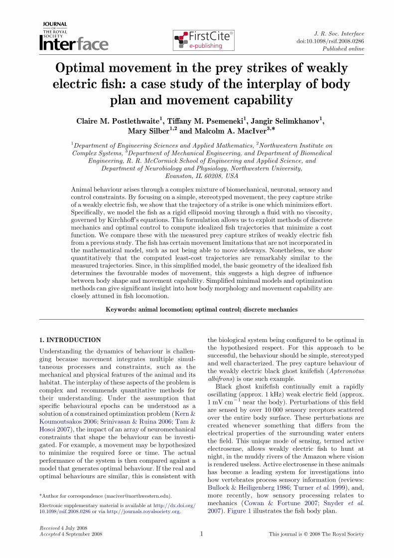
Figure 1.Body plan of fish and ellipsoidal model. The figure shows the outline of the ellipsoid model and a transparent body plan ofthe black ghost knifefish Apteronotus albifrons. Fish lengths varied from 12 to 15 cm. The length of the ellipsoid (2l1) is scaledsuch that the volumes of the fish and the ellipsoid match. Note that the ellipsoid is narrower than the fish at the front of the body,and wider than the fish at the rear of the body, with the consequent changes in the shading of the ellipsoid as it is covered by thesurface of the fish body. (a) The unbent fish and fitted volume-matched ellipsoid. (b) How the ellipsoid is oriented if the fish bodyis bent. The tip of the ellipsoid coincides with the location of the fish nose, and is oriented to coincide with the unbent rostral thirdof the fish.

2 Optimal movement in weakly electric fish C. M. Postlethwaite et al.

Prior work has shown that the volume in which preyare detected (approx. 3 cm out in all directions from thebody surface) is similar in size and shape to the volumewhich the animal needs to come to a halt to capture theprey (Snyder et al. 2007). A rapid and precise strikemust therefore be initiated almost immediately upondetection—otherwise, the prey will rapidly pass out ofthe sensory volume. Given this, and under theassumption that energy cost is proportional to musclework, we expect that strikes will be strongly con-strained by mechanical factors and that optimization ofan appropriately chosen mechanical utility functionmay be predictive of the behaviour.

The kinematics of the weakly electric fish’s prey strikehas been systematically examined empirically using anapproach that gives the full three-dimensional positionof the body over time (MacIver et al. 2001). The resultsshow the behaviour to be highly stereotyped. The fishgenerally swims forward at approximately 10 cm sK1, inthe dark, using its electrosensory system to detect preyin all directions around the body up to approximately3 cm away. Only a small fraction of the prey are detectedahead of the body. In the majority of cases, the fishrapidly reverses its body (in z100 ms) to bring itsmouth to the detected prey.

In our highly abstracted approach, we do not modelthe way the fish generates propulsion. Propulsion inaquatic animals generally occurs through flapping of finsor body undulation. These movements impart momen-tum to the fluid, and are generally associated with thedevelopment of characteristic vortices in the wake of theswimmer. This has been observed in both experimentsand numerical simulations. A few examples includevortices shed at the trailing edges of anguilliformswimming (i.e. eels; Tytell & Lauder 2004), vortex ringsshed by jellyfish (Dabiri et al. 2005a,b) and knifefish(Shirgaonkar et al. in press), and vortex structuresgenerated by the pectoral fins of sunfish (Drucker &Lauder 1999). Weakly electric fish swim using a uniqueadaptation, an elongated ribbon-like anal fin along theventral midline of the body. Rather than bend theirbody for propulsion asmany fishes do, these fish generatetravellingwaves along their ribbonfin, oftenkeeping theirbody straight (Blake 1983; Lighthill & Blake 1990).By changing the direction, frequency, amplitude andnumber of waves on the fin, they can precisely control


the magnitude and direction of thrust (Shirgaonkar et al.in press). During exploration of novel objects or inconfined spaces, bodybends canoccur to facilitate sensingor for turning, and this bending is decoupled frompropulsion (Assad et al. 1999). The prey strikes we aremodelling are high-speed transient movements. Duringthese high-speedmovements, just as in steady swimming,the body is kept straight—or if it was bent prior toprey detection, it is rapidly straightened (MacIver et al.2001), presumably to maximize the surge force arisingfrom the streamwise jet generated by the ribbon fin(Shirgaonkar et al. in press).

Given these considerations, as well as significantmathematical advantages, we model the fish body as arigid ellipsoid with no fins—which is clearly unable togenerate the types of forces described earlier, which arerequired for locomotion. In our model, the fish ispropelled by forces and torques which act at the centreof mass of the body, but we do not describe how theseforces originate. Our model does not consider thecomplicated fluid mechanics underlying the propulsionmethods discussed above, but assumes only that thefish has some mechanism of generating thrust, and thatthe generation of this thrust has some cost to the fish.

As with most fishes, the motion capabilities of theknifefish are limited. More precisely, if a rigid bodycan actively move in all six degrees of freedom (surge,heave and sway translational motions, and yaw, pitchand roll rotational motions—see figure 2), it is saidto be ‘fully actuated’, while if it cannot it is ‘under-actuated’. As we will provide evidence for below, theknifefish can move forward, backward, heave upward,roll and pitch—but cannot yaw, sway or heave down-ward. Thus, it is underactuated.

In this paper, we test the hypothesis that thetrajectory of the fish body, as approximated by anappropriately sized rigid ellipsoid, minimizes mechan-ical effort. Importantly, we allow our idealized fish to befully actuated. If the fully actuated idealized bodyfollows the same trajectory as the underactuated realfish, this would be indirect evidence that the fish, eventhough underactuated, is sufficiently actuated to per-form optimal movements. Another way to express thepoint is that the fish has all the movement capability itneeds for effective low-cost movement. To provide moredirect evidence for this claim, we also underactuate the

–100 –50 0 50 100 150 200–80–60–40–20

020406080

Q (deg.)

F (

deg.

)

heave up (yaw left)

heave down (yaw right)

sway right(pitch up)

sway left(pitch down)

surge forward(roll right)

surgebackward(roll left)

surge

heave(a) (b)

(roll)

(yaw)

(pitch)sway

F

Q

Figure 2. Velocity vector representation. We show the representation for translational and rotational velocities simultaneously,with labels related to the rotational velocity representation shown in parentheses. (a) Representing the directions of the linear (v)and rotational (u) velocity vectors as points on the surface of a sphere. The six shaded circles are regions close to a coordinateaxis. If a vector intersects the sphere in one of the circles, it can be associated with a simple movement in the direction of or aboutthat axis. A linear velocity vector v corresponds to a translation in the direction of that vector. A rotational velocity vector ucorresponds to a rotation of the body about that axis. We show an example vector, denoted by v (u). (b) The spherical angles Qand F (defined in §2.1.1) as rectangular coordinates. The shaded regions correspond to those in (a) and are labelled according tothe type of translational (or, in parentheses, rotational) movement that is associated with the velocity vectors within thoseregions. The indicated point v (u) illustrates how a vector is mapped from the sphere shown in (a).

Optimal movement in weakly electric fish C. M. Postlethwaite et al. 3

idealized fish in some of the same ways that the real fishis underactuated, and examine whether there is anychange in the generated optimal trajectories. If theoptimal trajectories are essentially unchanged, then wecan conclude that those additional degrees of freedom arenot needed by the fish to achieve optimal movements.

This paper is organized as follows. In §2 we describeour simplified mechanical model of the fish and ouroptimization procedure. In §3 we apply our optimizationmethods to test three hypotheses. We find that ouroptimal trajectories match the measured trajectorieswith excellent agreement, suggesting that the fish indeedmoves so as to minimize effort. This is discussed in §3.1.Further in §3.2 we find that optimal trajectories for a fishmodel that was underactuated in the same way as thereal fish have little difference from the fully actuatedcase. The fish therefore has all the movement abilities itneeds for low-cost movements. Finally in §3.3 we showthat we can use the minimum-effort criterion to detect aswitch from prey search behaviour to the goal-directedbehaviour of a prey strike in a post hoc analysis. This issimply because, prior to prey detection, the fish is notattempting to reach a specific point in space (the oneoccupied by the prey) withminimal effort; we can use theonset of an optimal trajectory to that point as a methodfor detecting a behavioural mode switch. Section 4concludes the paper with a discussion of the results, thelimitations of our mechanical model and some sugges-tions of how wemight further investigate the motion andsensing capabilities of the weakly electric fish using toolsof mechanics and optimal control.

2. METHODS

In a previously published study (MacIver et al. 2001),adult weakly electric fish (A. albifrons) were videotapedin a light-tight enclosure under infrared illumination.Individual water fleas (Daphnia magna, 2–3 mm inlength) were introduced near the water surface anddrifted downward; prey capture behaviour was


recorded using a pair of video cameras oriented alongorthogonal axes. Relative to the fish’s velocity (approx.10 cm sK1), the prey were relatively stationary (preyvelocity less than 2 cm sK1). Prey capture events (fromshortly before detection to capture) were subsequentlydigitized, and three-dimensional motion trajectories ofthe fish surface and prey were obtained using a model-based tracking system with a spatial resolution of0.5 mm and a temporal resolution of 1/60 s (MacIver &Nelson 2000). The time of prey detection (tD) wasdefined by the onset of an abrupt longitudinaldeceleration as the fish reversed swimming directionto capture the prey. These reversals are characteristicof most prey capture encounters. Initial prey sensingtends to be uniformly distributed along the entirelength of the body, so a reversal of swimmingdirection is typically required to intercept the prey.A total of 116 prey capture manoeuvres (hereafter,‘trials’) were recorded.

In our optimization procedure, we use an idealizedmodel of the fish in which we model the body as a solidrigid ellipsoid. In order to compare mechanicallyoptimal trajectories with the video-captured fishtrajectories described above, we fit a trajectory of anellipsoid to the video-captured data. Four fish ofslightly different sizes were used in the prey capturestudy (MacIver et al. 2001). For each prey capture trial,the corresponding model ellipsoid has the same width(2l2) and height (2l3) as the fish, but the length (2l1) ofthe ellipsoid is chosen such that the volumes of thefish and ellipsoid are equal. This results in an ellipsoidwith approximately 67 per cent of the length of the fish.We assume the fish is neutrally buoyant, so the densityof the ellipsoid is equal to that of the surrounding fluid.Equal volumes of the fish and ellipsoid then also resultin equal masses. For the four fish that were used in theprey capture study, the model ellipsoids have semi-axeslengths l1 ranging from 4.06 to 5.05 cm, l2 from 0.39 to0.46 cm and l3 from 0.85 to 1.08 cm.


The data from the digitized motion capture eventsgive the coordinates of the fish nose in a laboratory-fixed frame, and three angles that describe theorientation of the fish body, as functions of time. Wecreate an approximation to the fish’s trajectory byfitting the ellipsoid model to the trajectory of the fish.For each time step of the recorded behaviour, weposition the ellipsoid so that the front of the ellipsoidand the fish nose coincide, and orient the ellipsoid sothat the rostral part of the fish and the ellipsoid arealigned, as shown in figure 1. Throughout the paper, werefer to this rigid ellipsoid-fitted trajectory as the‘motion-capture fitted (MCF) trajectory.’

In comparisons between mechanically optimal andMCF trajectories, each of the two ellipsoids isrepresented by a surface mesh of 256 nodes. Weevaluate the distance between corresponding nodes toobtain a measure of how similar the two trajectoriesare. Details of this error measure calculation can befound in §2.4.

We next describe how the optimal trajectories arecomputed, beginning with a description of how we modelthe hydrodynamics of the submerged ellipsoidal approxi-mation to the fish. We then describe the optimizationprocedure, the objective function that is to be minimizedand the constraints on the optimization.

2.1. Equations of motion

The fish is modelled as a neutrally buoyant solid rigidellipsoid immersed in an infinitely large volume ofincompressible, inviscid fluid that is at rest at infinity.For Reynolds numbers typical of the fish motions(103–104) (Blake 1983; Shirgaonkar et al. in press), theinviscid assumption is reasonable. In some trials, owingto the small behavioural tank the original study wasconducted in, the fish is bent prior to prey detection. Asdiscussed in §1, this bending is not part of the fish’spropulsion mechanism. We discuss the bending of thefish and how we exclude such trials from our compari-son in §2.3.

It is well known (Lamb 1932) that the motion of suchan ellipsoid through an ideal fluid can be describedusing the Kirchhoff equations

M _v ZMv!uCF; ð2:1ÞJ _uZ Ju!uCMv!vCT ; ð2:2Þ

where v and u are three-vectors describing the velocityof the centre of mass of the ellipsoid and the angularvelocity of the body, respectively. The matrices M andJ are the effective mass and moment of inertia(discussed further below), and F and T are appliedforces and torques.

Recall that we do not discuss the origin of the appliedforces and torques, but only assume that they aregenerated by the fish, and producing forces in differentdirections costs the fish the same amount of effort. Wecan write FðtÞZðF1ðtÞ;F2ðtÞ;F3ðtÞÞ and TðtÞZðT1ðtÞ;T2ðtÞ;T3ðtÞÞ where F1 is the surge force, F2 is thesway force and F3 is the heave force, and T1 is the rolltorque, T2 is the pitch torque and T3 is the yaw torque.In this formulation, the forces and torques act atthe centre of mass of the body. Moreover, we allow the


body to be fully actuated, i.e. F(t) and T(t) can be anythree-vectors.

Since we assume the fluid is inviscid, this modeldoes not include the effects of drag. We discuss reasonswhy this is not expected to significantly affect ourresults in §4.

All quantities in equations (2.1) and (2.2) are givenin a frame of reference which rotates with the body. Werefer to this frame as the ‘body frame’, and to a fixedinertial frame of reference as the ‘laboratory frame’. Wechoose the body frame so the x -axis is aligned with thelong axis of the fish, as shown in figure 1. The matricesM and J are given by

M Z

m1 0 0

0 m2 0

0 0 m3

0B@

1CA; J Z

j1 0 0

0 j2 0

0 0 j3

0B@

1CA; ð2:3Þ

where M is the sum of the added mass matrix (due tothe volume of fluid accelerated by translations of theellipsoid) and the body mass matrix, and J is the sum ofthe added moment of inertia matrix (due to the volumeof fluid accelerated by rotations of the ellipsoid) and thebody moment of inertia matrix. Formulae to calculatemi and ji can be found in Holmes et al. (1998). Recallthat we use four model ellipsoids of slightly differentsizes in our calculations. For one of our four ellipsoidmodels, we find (m1, m2, m3)Z(6.04, 17.31, 8.39) g,( j1, j2, j3)Z(1.57, 27.78, 54.11) g cm2 and the mass ofthe ellipsoid,mZ5.84 g. The other three ellipsoids havesimilar values. The fluid motion enters the model onlythrough the added mass and inertia effects.

The position and orientation of the body withrespect to the laboratory frame are given by a three-vector b, which gives the position of the centre of massof the body, and a rotation matrix R, which we write interms of three Euler angles f, q and j (R is given interms of these angles in appendix A). We choose theEuler angles so that f is a rotation about the x -axis(roll), q is a rotation about the y-axis (pitch) and j is arotation about the z -axis (yaw). Note that the Eulerangles themselves do not give useful information forvisualizing the orientation of the fish, since if more thanone of the Euler angles is non-zero the fish has undergonea combination of rotations. Rotations of the fish arebetter understood by examining the form of the angularvelocity vector u. We discuss this further along with ourmethod of representing the rotations of the fish in §2.1.1.The choice of the Euler angles we make has singularitiesat qZG908, and so we restrict q2(K908Ce, 908Ke) forsome 0!e/1808. (Typically we choose ez68. Norestrictions are required on the other angles.)

The body-frame velocity v and angular velocity u arerelated to the state variables in _b and R by

v ZRK1 _b; _RZRu; ð2:4Þ

where if uZ(u1, u2, u3), then u is the matrix

uZ

0 Ku3 u2

u3 0 Ku1

Ku2 u1 0

0B@

1CA: ð2:5Þ


Equations (2.1)–(2.4) with prescribed forces andtorques F(t) and T(t), together with initial conditionsb(tI)Zb0, R(tI)ZR0, v(tI)Zv0 and u(tI)Zu0, fullydescribe the motion of the body through the fluid fortOtI. In the following, we refer to the trajectory interms of the state variables as a vector qðtÞZðbðtÞ;fðtÞ; qðtÞ;jðtÞÞ.

2.1.1. Velocity classifications. In the discussion of themotion of three-dimensional rigid objects, it is oftenconvenient to refer to velocities in simple terms such as‘heave’, ‘pitch’, ‘roll’, etc. Generic velocity vectors vand u cannot, however, be classified as such—theinstantaneous linear or rotational velocity of the bodywill be a complicated combination of several of thesemotions. In §3, however, we find it useful to classify thevelocity vectors into such categories whenever possible,as described below.

Since the velocities v and u are given in the body-fixed frame of reference shown in figure 1, if the vectorsare close to one of the coordinate axes, they can beassociated with what we term ‘simple’ translations orrotations. That is, translational velocity vectors closeto one of the coordinate axes are associated with thesimple translations ‘surge’ in the x -direction, ‘sway’ inthe y-direction and ‘heave’ in the z -direction. Similarly,rotational velocity vectors close to one of the coordinateaxes are approximately rotations about one of theprimary body axes: ‘roll’ about the x -axis; ‘pitch’about the y-axis; and ‘yaw’ about the z -axis. Thesesimple rotations correspond to varying just one of theEuler angles.

By plotting the velocity vectors using sphericalcoordinates (R, Q, F) instead of Cartesian coordinates,we construct a two-dimensional representation for eachof the linear and angular velocity vectors. Each vector vcan be written vZRðcos Q cos F; sin Q cos F; sin FÞwhere K1308%Q!2308 is the azimuthal angle andK908%F%908 is the polar angle measured from thexy-plane. (Q and F can be thought of as longitude andlatitude, respectively, for a projection of the vectorsonto a sphere.) The regions of the two-dimensional(Q, F)-space corresponding to the simple translationsand rotations are highlighted in figure 2. We usethis representation of the velocity vectors throughoutthis paper.

2.2. Optimization procedure

For a given trajectory q(t), with t2[tI,tF], describingthe motion of the ellipsoid through the fluid, andassociated forces and torques F(t) and T(t), we canassociate a cost C

C Z

ðtFtI

KðqðtÞ; _qðtÞ;FðtÞ;TðtÞÞdt; ð2:6Þ

for some function K, given below. The computation ofthe mechanically optimal trajectories is a constrainedoptimization problem: minimize the cost function C,subject to constraints on the trajectory q(t). Theconstraints consist of the equations of motion(equations (2.1) and (2.2)) as well as boundary


conditions, and, if desired, further constraints on theapplied forces and torques. The boundary conditionsand further constraints are discussed in §2.2.1. Notethat the duration (tFKtI) of the trajectory is fixed.

The objective function we choose to be minimizedcan be thought of as a proxy for the metabolic cost ofmuscle activation for the fish to complete the tra-jectory. Our approach, which models the fluid asinviscid, does not lend itself to the use of an energy-based cost function. We choose an objective functionsimilar to that used by Kanso & Marsden (2005),

KðqðtÞ; _qðtÞ;FðtÞ;TðtÞÞZX3iZ1

FiðtÞ2 CðaiTiðtÞÞ2:

ð2:7ÞThe scaling factors ai are included so that the terms inthe sum have the same dimension, and are equal to thereciprocals of the radii of gyration of the ellipsoid. Forour model ellipsoids, ai range from 0.26 to 1.93 cmK1.

In order to implement the optimization, the tra-jectory q(t) has to be discretized. We achieve this byapproximating q(t) by a piecewise linear function on anevenly spaced time grid ft IZt0; t1;.; tNK1Z tFg.That is,

qðtÞZ qn CtK tn

tnC1K tnðqnC1KqnÞ

for t 2 ½tn; tnC1�; n Z 0;.;NK2: ð2:8Þ

The equations of motion (which form constraints on theoptimization) must also be discretized. The discretiza-tion of both the trajectory and the equations of motionis discussed further in appendix A.

The optimization is performed using the packageSNOPT (Gill et al. 2002), an implementation of sequen-tial quadratic programming (SQP). The optimizationroutine finds a local minimum, subject to any number ofconstraints, of the objective function, given an ‘initialguess’ trajectory qinit(t). We discuss the sensitivity ofthe routine to choosing different qinit(t) in §2.2.2.

2.2.1. Constraints.The optimization of the cost functionC is performed by varying the state variables q(t) andthe applied forces and torquesF(t) andT(t). Throughoutthe paper, the equations of motion are constraintson the optimization procedure, but, for each of thethree hypotheses described in the introduction, we use adifferent set of additional constraints, as follows.

For the first hypothesis, that the fish trajectories areclose to mechanically optimal, we set the start time ofthe trajectory to be the time of prey detection (definedin §2), so tIZtD, and the final time of the trajectory tobe that of prey capture. (Recall that the duration of thetrajectory is fixed to match that of the motion capturedata.) Boundary conditions are chosen so the trajectorycan be compared with the motion capture data (theMCF trajectory). Here, we fix the initial (that is, attZtI) position, orientation and both linear and angularvelocities of the trajectory to match that of the motioncapture data. That is, q(tI) and _qðt IÞ are given. In thisstudy, we also fix q(tF) (the final position andorientation of the ellipsoid) to that of the MCFtrajectory, but _qðtFÞ is free to vary.

02

–150

–100

–50

0

50

468

10121416182022(a) (b)

0.1

posi

tion

of c

entr

eof

mas

s (c

m)

0.2 0.3 0.4time from detection (s)

0.5 0.6 0.7 0.8 0 0.1 0.2 0.3

Eul

er a

ngle

s (d

eg.)

0.4time from detection (s)

0.5 0.6 0.7 0.8

Figure 3.Optimal trajectories as N is varied. Optimal trajectories obtained for one trial, for variousN. HereNZ5 is shown by thedotted curves, NZ10 the dot-dashed curves, NZ20 the dashed curves and NZ40 the solid curves. As N is increased(N2{5,10,20,40}), the optimal trajectories converge to the same solution. (a) Position of centre of mass. (b) Euler angles.


For the second hypothesis, concerning the redundantand essential motor capacities, we produce twoadditional sets of trajectories that we term ‘redundantlyunderactuated’ (RUA) and ‘essentially underactuated’(EUA). The initial and final times of these trajectoriesand the boundary conditions on the position andvelocity of the ellipsoid at these times are the same asfor the first hypothesis, given earlier. However, weimpose additional constraints on the allowed forces andtorques for both the RUA and EUA trajectories. Theseare described in detail in §3.2.

For our third hypothesis, to determine whether achange in behaviour can be detected using optimalcontrol results, we produce optimal trajectories forwhich the initial time tI is not equal to the time ofdetection tD. The final time of the trajectory remainsequal to the time of prey capture. In this study, weadditionally fix the velocity of the ellipsoid at tZtF tobe that of the MCF trajectory. That is, q(tI), _qðt IÞ, q(tF)and _qðtFÞ are given.

2.2.2. Validation. The results of the optimization codedescribed above give only approximate solutions to theKirchhoff equations, owing to the discretization of boththe equations and the trajectory. Ideally, we would runthe optimization code with a very large N (the numberof discretized time intervals), but this is not possibledue to finite computing power. Here we describe how wechoose an appropriate N.

For 10 randomly chosen trials (out of the 116 motioncapture trials), we produced optimal trajectories forN2{5,10,20,40,80} using the MCF trajectory as theinitial guess qinit(t). The results from one of these trialscan be seen in figure 3. Note that the CPU time requiredto produce the optimal trajectories increases exponen-tially with N since both the number of constraints andthe number of variables increase with N.

The optimal trajectory clearly converges as N isincreased. We determine the N values for which theoptimal solutions are sufficiently discretized bycomparing the solutions with two different discretiza-tions of the Kirchhoff equations. As N increases, weexpect that the discrepancies between the solutions fordifferent discretizations will decrease to zero.


We set a discrepancy level using the following twocomparisons. First, using the functions F(t) and T(t)from the optimal trajectory, we obtained a correspond-ing q(t) by forward integrating equations (2.1)–(2.4)using a built-in Runge–Kutta (4,5) solver in MATLAB

(The Mathworks, Natick, MA, USA). This output wascompared with the q(t) provided by the optimizationcode. Second, we implemented a different discretizationof Kirchhoff’s equations (from that used as constraintsfor the optimization): we solved equations (2.1) and(2.2) for F(t) and T(t) using (the discretized) v(t) andu(t) from the optimal trajectory. This was comparedwith F(t) and T(t) provided by the optimization code.

For N ranging between 5 and 80, we found that, onaverage (for the 10 trials chosen above), the discrepancymeasure we used decreased by an order of magnitudeeach time N was doubled. We set an allowed tolerancelevel for this discrepancy measure, and found that, formost trials, NZ40 produced optimal solutions thatpassed this discrepancy check. Seven trials (out of 116)were excluded from the rest of our calculations becausethey did not meet our tolerance level on these checks.

For the same 10 trials used in our convergence testsdescribed above, we also investigated the robustness ofthe optimization results to different initial guesstrajectories qinit(t). This can indicate whether thecode is finding a local or global optimum. In additionto the MCF trajectory, we used three other types ofinitial guess trajectories, as follows: a straight linebetween the boundary conditions for each of the statevariables ðbðtÞ;fðtÞ; qðtÞ;jðtÞÞ; a quadratic polynomialconsistent with the boundary conditions; and atrajectory created by adding random noise (rangingup to 10%) to the MCF trajectory and then smoothingusing a low-pass digital Butterworth filter. For each ofthe different qinit(t) used, we found that the codeproduced an optimal solution that was almost identicalto the optimal solution produced using the MCFtrajectory as the initial guess: the maximum error was1.76!10K5 cm in position and 0.00178 in orientation.The optimization scheme (SNOPT, see §2.5) only findslocally optimal solutions, but the results of thisvalidation check provide convincing evidence thatthe solution obtained is the global minimum to theobjective function. In the following results, we usethe MCF trajectory as the initial guess qinit(t).

0.2 0.3 0.4 0.5 0.6 0.7 0.8 0.9 1.0 1.1 1.20

5

10

15

20

25

measure of bend

no. o

f tr

ials

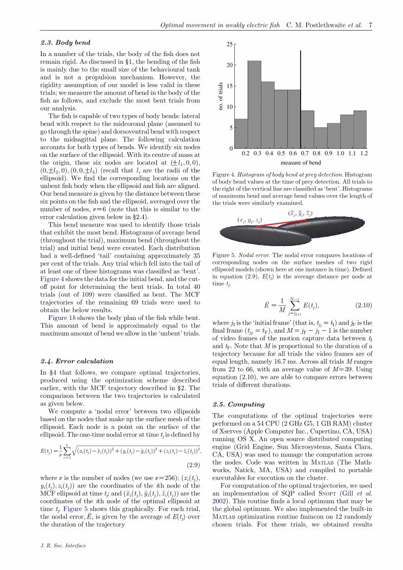
Figure 4.Histogram of body bend at prey detection. Histogramof body bend values at the time of prey detection. All trials tothe right of the vertical line are classified as ‘bent’. Histogramsof maximum bend and average bend values over the length ofthe trials were similarly examined.

Figure 5. Nodal error. The nodal error compares locations ofcorresponding nodes on the surface meshes of two rigidellipsoid models (shown here at one instance in time). Definedin equation (2.9), E(tj) is the average distance per node at


2.3. Body bend

In a number of the trials, the body of the fish does notremain rigid. As discussed in §1, the bending of the fishis mainly due to the small size of the behavioural tankand is not a propulsion mechanism. However, therigidity assumption of our model is less valid in thesetrials; we measure the amount of bend in the body of thefish as follows, and exclude the most bent trials fromour analysis.

The fish is capable of two types of body bends: lateralbend with respect to the midcoronal plane (assumed togo through the spine) and dorsoventral bendwith respectto the midsagittal plane. The following calculationaccounts for both types of bends. We identify six nodeson the surface of the ellipsoid. With its centre of mass atthe origin, these six nodes are located at ðGl 1; 0; 0Þ;ð0;Gl 2; 0Þ; ð0; 0;Gl 3Þ (recall that l i are the radii of theellipsoid). We find the corresponding locations on theunbent fish body when the ellipsoid and fish are aligned.Our bendmeasure is given by the distance between thesesix points on the fish and the ellipsoid, averaged over thenumber of nodes, nZ6 (note that this is similar to theerror calculation given below in §2.4).

This bend measure was used to identify those trialsthat exhibit the most bend. Histograms of average bend(throughout the trial), maximum bend (throughout thetrial) and initial bend were created. Each distributionhad a well-defined ‘tail’ containing approximately 35per cent of the trials. Any trial which fell into the tail ofat least one of these histograms was classified as ‘bent’.Figure 4 shows the data for the initial bend, and the cut-off point for determining the bent trials. In total 40trials (out of 109) were classified as bent. The MCFtrajectories of the remaining 69 trials were used toobtain the below results.

Figure 1b shows the body plan of the fish while bent.This amount of bend is approximately equal to themaximumamount of bendwe allow in the ‘unbent’ trials.

2.4. Error calculation

In §4 that follows, we compare optimal trajectories,produced using the optimization scheme describedearlier, with the MCF trajectory described in §2. Thecomparison between the two trajectories is calculatedas given below.

We compute a ‘nodal error’ between two ellipsoidsbased on the nodes that make up the surface mesh of theellipsoid. Each node is a point on the surface of theellipsoid. The one-time nodal error at time tj is defined by

EðtjÞZ1

n

XniZ1

ffiffiffiffiffiffiffiffiffiffiffiffiffiffiffiffiffiffiffiffiffiffiffiffiffiffiffiffiffiffiffiffiffiffiffiffiffiffiffiffiffiffiffiffiffiffiffiffiffiffiffiffiffiffiffiffiffiffiffiffiffiffiffiffiffiffiffiffiffiffiffiffiffiffiffiffiffiffiffiffiffiffiffiffiffiffiffiffiffiffiffiffiffiffiffiffiffiffiffiffiffiffiffiffiffiffiðxiðtjÞK~xiðtjÞÞ2CðyiðtjÞK~yiðtjÞÞ2CðziðtjÞK~ziðtjÞÞ2

q;

ð2:9Þ

where n is the number of nodes (we use nZ256); ðxiðtjÞ;yiðtjÞ; ziðtjÞÞ are the coordinates of the ith node of theMCF ellipsoid at time tj; and ð~xiðtjÞ; ~yiðtjÞ; ~ziðtjÞÞ are thecoordinates of the ith node of the optimal ellipsoid attime tj. Figure 5 shows this graphically. For each trial,the nodal error, �E, is given by the average of E(tj) overthe duration of the trajectory


�E Z1

M

XjFK1

jZj IC1

EðtjÞ; ð2:10Þ

where jI is the ‘initial frame’ (that is, tj IZ tI) and jF is thefinal frame ðtjFZ tFÞ, andMZ jFK jIK1 is the numberof video frames of the motion capture data between tIand tF. Note that M is proportional to the duration of atrajectory because for all trials the video frames are ofequal length, namely 16.7 ms. Across all trials M rangesfrom 22 to 66, with an average value of MZ39. Usingequation (2.10), we are able to compare errors betweentrials of different durations.

time tj.

2.5. Computing

The computations of the optimal trajectories wereperformed on a 54 CPU (2 GHz G5, 1 GB RAM) clusterof Xserves (Apple Computer Inc., Cupertino, CA, USA)running OS X. An open source distributed computingengine (Grid Engine, Sun Microsystems, Santa Clara,CA, USA) was used to manage the computation acrossthe nodes. Code was written in MATLAB (The Math-works, Natick, MA, USA) and compiled to portableexecutables for execution on the cluster.

For computation of the optimal trajectories, we usedan implementation of SQP called SNOPT (Gill et al.2002). This routine finds a local optimum that may bethe global optimum. We also implemented the built-inMATLAB optimization routine fmincon on 12 randomlychosen trials. For these trials, we obtained results

(b)(a) (c) (d ) (e) ( f )

0

5

10

15

20

25

posi

tion

of c

entr

e of

mas

s (c

m)

0 0.1 0.2 0.3 0.4 0.5 0.6 0.7 0.8–250

–200

–150

–100

–50

0

50

100

time from detection (s)

Eul

er a

ngle

s (d

eg.)

(a)

(b)

(c)

(d )

(e)

( f )

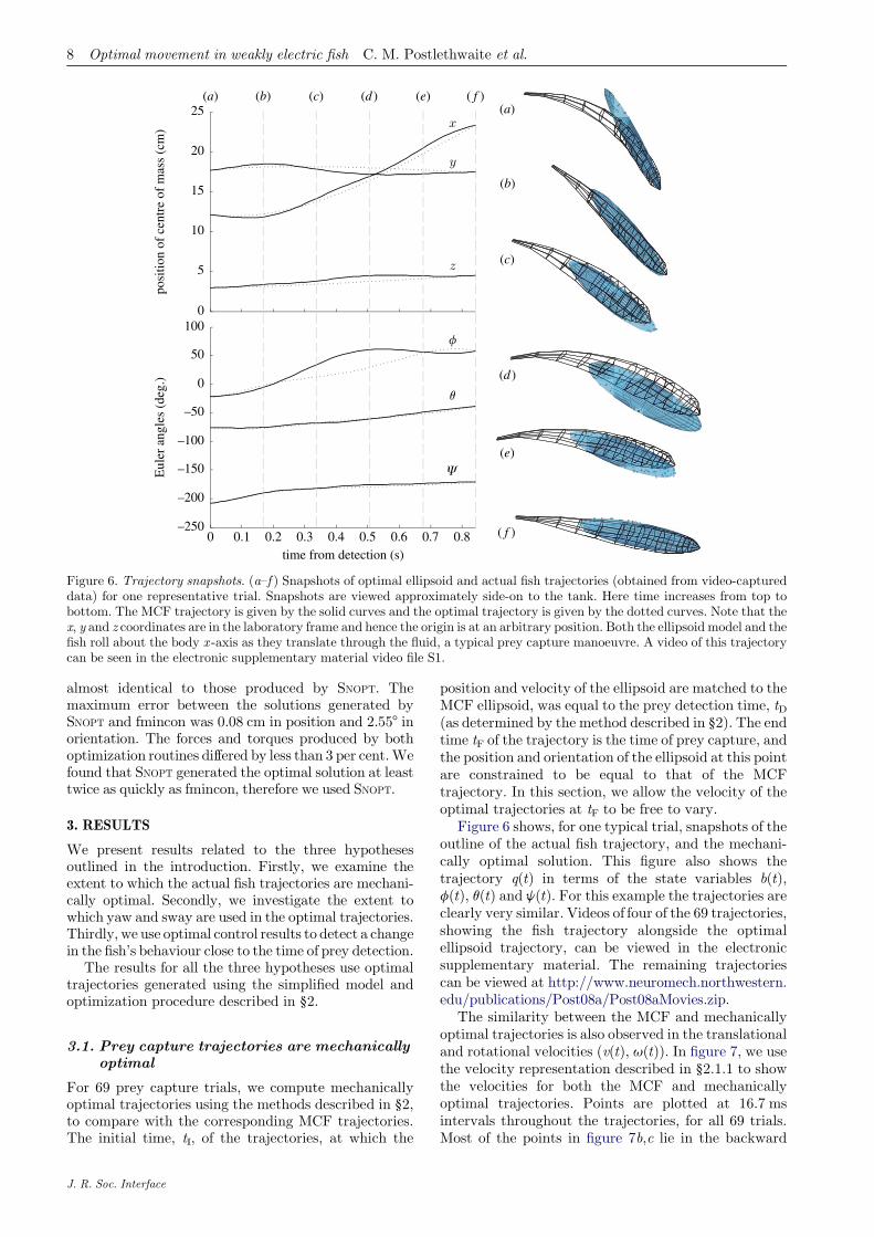
Figure 6. Trajectory snapshots. (a–f ) Snapshots of optimal ellipsoid and actual fish trajectories (obtained from video-captureddata) for one representative trial. Snapshots are viewed approximately side-on to the tank. Here time increases from top tobottom. The MCF trajectory is given by the solid curves and the optimal trajectory is given by the dotted curves. Note that thex, y and z coordinates are in the laboratory frame and hence the origin is at an arbitrary position. Both the ellipsoid model and thefish roll about the body x -axis as they translate through the fluid, a typical prey capture manoeuvre. A video of this trajectorycan be seen in the electronic supplementary material video file S1.


almost identical to those produced by SNOPT. Themaximum error between the solutions generated bySNOPT and fmincon was 0.08 cm in position and 2.558 inorientation. The forces and torques produced by bothoptimization routines differed by less than 3 per cent.Wefound that SNOPT generated the optimal solution at leasttwice as quickly as fmincon, therefore we used SNOPT.

3. RESULTS

We present results related to the three hypothesesoutlined in the introduction. Firstly, we examine theextent to which the actual fish trajectories are mechani-cally optimal. Secondly, we investigate the extent towhich yaw and sway are used in the optimal trajectories.Thirdly, we use optimal control results to detect a changein the fish’s behaviour close to the time of prey detection.

The results for all the three hypotheses use optimaltrajectories generated using the simplified model andoptimization procedure described in §2.

3.1. Prey capture trajectories are mechanicallyoptimal

For 69 prey capture trials, we compute mechanicallyoptimal trajectories using the methods described in §2,to compare with the corresponding MCF trajectories.The initial time, tI, of the trajectories, at which the


position and velocity of the ellipsoid are matched to theMCF ellipsoid, was equal to the prey detection time, tD(as determined by the method described in §2). The endtime tF of the trajectory is the time of prey capture, andthe position and orientation of the ellipsoid at this pointare constrained to be equal to that of the MCFtrajectory. In this section, we allow the velocity of theoptimal trajectories at tF to be free to vary.

Figure 6 shows, for one typical trial, snapshots of theoutline of the actual fish trajectory, and the mechani-cally optimal solution. This figure also shows thetrajectory q(t) in terms of the state variables b(t),f(t), q(t) and j(t). For this example the trajectories areclearly very similar. Videos of four of the 69 trajectories,showing the fish trajectory alongside the optimalellipsoid trajectory, can be viewed in the electronicsupplementary material. The remaining trajectoriescan be viewed at http://www.neuromech.northwestern.edu/publications/Post08a/Post08aMovies.zip.

The similarity between the MCF and mechanicallyoptimal trajectories is also observed in the translationaland rotational velocities (v(t), u(t)). In figure 7, we usethe velocity representation described in §2.1.1 to showthe velocities for both the MCF and mechanicallyoptimal trajectories. Points are plotted at 16.7 msintervals throughout the trajectories, for all 69 trials.Most of the points in figure 7b,c lie in the backward

http://www.neuromech.northwestern.edu/publications/Post08a/Post08aMovies.zip

http://www.neuromech.northwestern.edu/publications/Post08a/Post08aMovies.zip

70 190 310 430 550

vector magnitude (deg s–1)

yaw left

yaw right

pitchup

pitchdown

rollright

rollleft

–100 –50 0 50 100 150 200–80–60–40–20

020406080

(deg.)–100 –50 0 50 100 150 200

5 10 15 20 25

vector magnitude (cm s–1)

–80–60–40–20

020406080(a)

(b)

(c)

(d )

(e)

( f )

heave up

heave down

swayright

swayleft

surgeforward

surgebackward

–80–60–40–20

020406080

(deg.)

(de

g.)

(de

g.)

(de

g.)

Figure 7. Velocity vectors for all trials. (a–c) Translational and (d–f ) rotational velocities for the MCF and the mechanicallyoptimal trajectories, for all 69 trials. Figure 2 shows how the figures are generated. The colour bar corresponds to the magnitudesof the velocity vectors (cm sK1 for v(t) and deg sK1 for u(t)); velocities with the smallest magnitudes (25% of the data) have beenomitted here. Both (b) and (c) show clustering of points in the surge and upward heave regions and a lack of points in the sway anddownward heave regions. In (e) and ( f ), clustering is seen in the roll regions, but points are sparse in the yaw regions. (b,e) MCFand (c, f ) optimal.


surge region, which indicates that the optimal tra-jectories exhibit the same rapid-reversal manoeuvre thatis typically observed in the fish’s prey capture behaviour(MacIver et al. 2001). A concentration of points near thetop of the forward surge region can also be seen. Thiscorresponds to an upward heave during forwardtranslation. It is important to note the lack of points inboth the sway regions and the heave down region. This isconsistent with our understanding that the fish does notpossess the means to produce force or torque in thesedirections. A clustering of points is clearly visible in theroll regions in both figure 7e and figure 7f. There are veryfew points in the regions for yaw, a body rotation thatthe fish is not capable of performing. We examine theyaw and sway abilities in more detail in §3.2.

We calculate the nodal error, �E (as described in§2.4), between the MCF ellipsoid and mechanicallyoptimal trajectories over all 69 trials. The mean nodalerror is 1.31 cm with a standard deviation of 0.58 cm.We note that the mean nodal error for the 40 bent trialsis not significantly different: 1.38 cm with a standarddeviation of 0.50 cm.

We compare the mean nodal error for the mechani-cally optimal results to two length scales of the fishmotion. These length scales are the length of theellipsoids, and the total (integrated) distance travelled


by the centre of mass of the fish during the trajectory(from the time of prey detection to capture). The averagelength of the model ellipsoids is 9 cm (which is onlyapprox. 67% of the actual fish body length), and theaverage distance travelled by the fish is approximately8 cm. The mean nodal error (1.31 cm) is much smallerthan both of these. We note further that the range ofdistances travelled is large (3.5–16.8 cm), and there is nosignificant correlation between the distance travelled andthe nodal error across the trials. Since the error is smallcompared with typical length scales of the motion, weassert that the trajectories are similar, and so the MCFtrajectories are therefore close to being mechanicallyoptimal. Since the MCF trajectories are a closeapproximation of the actual motion of the fish, the fishtrajectories are also close to being mechanically optimal.

3.2. Distinguishing essential and redundantmotor capacities using optimal trajectories

As previously noted in §3.1, the prey capture trajectorymotions do not contain much sway or yaw motion.This can be seen in the MCF trajectories shown infigure 7. The dominant motions seen are surge androll. The mechanically optimal results also showsimilar patterns.

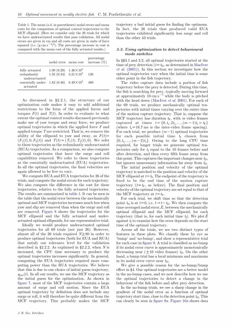
Table 1. The mean (s.d. in parentheses) nodal errors and meancosts for the comparison of optimal control trajectories to theMCF ellipsoid. (Here we consider only the 26 trials for whichwe have underactuated results that pass validation. All nodalerrors are given in cm and all costs are given in units of forcesquared (i.e. (g cm sK2)2). The percentage increase in cost iscompared with the mean cost of the fully actuated results.)

nodal error mean costpercentageincrease (%)

fully actuated 1.00 (0.29) 1.46!105

redundantlyunderactuated

1.35 (0.34) 3.21!105 120

essentially under-actuated

1.82 (0.46) 8.49!105 480


As discussed in §2.2.1, the structure of ouroptimization code makes it easy to add additionalrestrictions to the form of the applied forces andtorques F(t) and T(t). In order to evaluate to whatextent the optimal control results discussed previouslymake use of yaw torque and sway force, we produceoptimal trajectories in which the applied force F andapplied torque T are restricted. That is, we remove theability of the ellipsoid to yaw and sway, so FðtÞZðF1ðtÞ; 0;F3ðtÞÞ and TðtÞZðT1ðtÞ;T2ðtÞ; 0Þ. We referto these trajectories as the redundantly underactuated(RUA) trajectories. As a comparison, we also computeoptimal trajectories that have the surge and rollcapabilities removed. We refer to these trajectoriesas the essentially underactuated (EUA) trajectories.In all the optimal trajectories, the final velocities areagain allowed to be free to vary.

We compute RUA and EUA trajectories for 26 of thetrials, and compute the nodal errors for each trajectory.We also compute the difference in the cost for thesetrajectories, relative to the fully actuated trajectories.The results are summarized in table 1. It can be seen inthe table that the nodal error between the mechanicallyoptimal and MCF trajectories increases much less whenyaw and slip are removed than when the surge and rollare removed. Figure 8 shows the trajectories for theMCF ellipsoid and the fully actuated and under-actuated optimal ellipsoids, for one representative trial.

Ideally we would produce underactuated optimaltrajectories for all 69 trials (not just 26). However,almost all of the 26 trials required NR80 in order toproduce optimal trajectories (both for EUA and RUA)that satisfy our tolerance level for the validationdescribed in §2.2.2. As explained in §2.2.2, when N isincreased, the CPU time necessary to produce theoptimal trajectories increases significantly. In general,computing the EUA trajectories required more com-puting power than the RUA trajectories. We believethat this is due to our choice of initial guess trajectory,qinit(t). In all our results, we use the MCF trajectory asthe initial guess for the optimization. As shown infigure 7, most of the MCF trajectories contain a largeamount of surge and roll motion. Since the EUAoptimal trajectory by definition does not include anysurge or roll, it will therefore be quite different from theMCF trajectory. This probably makes the MCF


trajectory a bad initial guess for finding the optimum.In fact, the 26 trials that produced valid EUAtrajectories exhibited significantly less surge and rollthan the other 43 trials.

3.3. Using optimization to detect behaviouralmode switches

In §§3.1 and 3.2, all optimal trajectories started at thetime of prey detection (tZtD, as determined in MacIveret al. (2001)). In this section we investigate how theoptimal trajectories vary when the initial time is someother point in the fish trajectory.

The video capture data include a portion of fishtrajectory before the prey is detected. During this time,the fish is searching for prey, typically moving forwardat approximately 10 cm sK1 while the body is pitchedwith the head down (MacIver et al. 2001). For each ofthe 69 trials, we produce mechanically optimal tra-jectories with initial times varying over the entire timeof the motion capture trajectory. That is, suppose theMCF trajectory has duration tF, with m video framescaptured at times tZf0; ts; 2ts;.; ðmK1ÞtsZ tFg(where tsZ16.7 ms is the inter-video frame spacing).For each trial, we produce (mK1) optimal trajectoriesfor each possible initial time tI chosen fromf0; ts;.; ðmK2Þtsg. Owing to the long CPU timerequired, for longer trials we generate optimal tra-jectories only for tI equal to the 10 frames before andafter detection, and then every fifth frame away fromthis point. This captures the important changes near tD,but ignores unnecessary information far away from tD.

The initial position and velocity of the optimaltrajectory is matched to the position and velocity of theMCF ellipsoid at tZtI. The endpoint of the trajectory isfixed to be the end time of the motion capturetrajectory (tZtF, as before). The final position andvelocity of the optimal trajectory are set equal to that ofthe MCF trajectory at tZtF.

For each trial, we shift time so that the detectionpoint tD is at tZ0, i.e. t/tKtD. We then compute thetime-averaged nodal error, �E, between the mechanicallyoptimal ellipsoid and the MCF ellipsoid, for eachtrajectory (that is, for each initial time tI). We plot �Eagainst tI to examine how the error depends on the starttime of the optimal trajectory.

Across all the trials, we see two distinct types offeatures in these plots. We classify these by eye as‘bump’ and ‘no-bump’, and show a representative trialfor each case in figure 9. A trial is classified as no-bumpif its nodal error curve is approximately monotonicallydecreasing near (G10 video frames) tD. On the otherhand, a bump trial has a local minimum and maximumin its nodal error curve near tD.

We give a possible reason for the no-bump/bumpeffect in §4. Our optimal trajectories are a better modelin the no-bump cases, and we now describe how we usethe optimal trajectories to detect a change in thebehaviour of the fish before and after prey detection.

In the no-bump trials, we see a sharp change in thegradient of the nodal error as a function of optimaltrajectory start time, close to the detection point tD. Thiscan clearly be seen in figure 9a. Figure 10a shows data

09

101112131415161718(a) (b)

0.1 0.2 0.3

posi

tion

of c

entr

eof

mas

s (c

m)

Eul

er a

ngle

s (d

eg.)

0.4time from detection (s)

0.5

MCF

RUA

EUA

optimal

0.6 0.7 0–200

–150

–100

–50

0

50

0.1 0.2 0.3 0.4time from detection (s)

0.5 0.6 0.7

Figure 8. Underactuated optimal trajectories. Trajectories for one representative trial for the MCF ellipsoid (solid black), thefully actuated optimal ellipsoid (dashed blue), the RUA ellipsoid (dotted red) and the EUA ellipsoid (dot-dashed green). TheRUA trajectory is clearly similar to the fully actuated trajectory, while the EUA trajectory is significantly different. (a) Positionof centre of mass. (b) Euler angles.

–15 –10 –5 00 0

0.5

1.0

1.5

2.0

2.5

3.0

3.5

0.2

0.4

0.6

0.8

1.0

1.2

1.4

1.6

1.8(a) (b)

5 10 15 20 25 30 –15 –10 –5 0 5initial time frameinitial time frame

10 15 20 25 30

E

Figure 9. Nodal error versus initial time frame. The nodal error between the optimal and MCF trajectories for one representativetrial (a) without and (b) with the post-detection bump.

–20 –15 –10 –5 00 0

0.20.40.60.81.01.21.41.61.82.0

0.5

1.0

1.5

2.0

2.5

3.0

initial time frame

5 10 15 20 –20 –15 –10 –5 0

initial time frame

5 10 15 20

(a) (b)

E

Figure 10. Mean nodal error versus initial time frame. Mean nodal error (shown with standard deviation bars) over all 69 trialsplotted versus the initial time frame relative to the detection time frame, for (a) no-bump and (b) bump trials.


averagedoverall theno-bumptrials, and the samechangein gradient can still be seen. We attribute the sharpchange in the gradient to a change in the fish’s behaviour.

Recall that we match the initial position, orientationand velocity of the optimal trajectory to the MCFtrajectory. Consider an optimal trajectory with initialtime tI pre-detection. We do not expect the optimal andMCF trajectories to be similar, since before preydetection the fish has no reason to move in an optimalfashion towards the prey. However, since the optimal


and MCF trajectories have initial and final positionsand velocities which are equal, it is expected that thenodal error would decrease as the trajectory durationdecreases (the nodal error is clearly zero when themotion-capture trajectory contains fewer than fiveframes as all the coordinates are completely constrainedby the initial and final conditions).

However, post-detection, when we expect the fish tofollow an optimal trajectory from its current position towhere the (relatively stationary) prey is sensed to be


located, we would not expect such a rapid decrease innodal error as trajectory duration decreases. This isbecause any post-detection portion of the MCFtrajectory is already close to mechanically optimal,according to the results already presented.

4. DISCUSSION

There have been a number of prior studies of animallocomotion using optimization techniques. Two dis-tinct methods are found in the literature. The first isparameter optimization, which is different from themethod we have used. This can be seen in Tam & Hosoi(2007) (who study a three-link swimmer in low-Reynolds number flow) and Kern & Koumoutsakos(2006) (studying anguilliform swimming). In thesestudies, there are a number of parameters that can bevaried, which may affect body shape, stroke pattern,etc. For a specific set of parameters, the resultingtrajectory is computed from the equations of motion,and this results in an output efficiency. The parameterscan then be varied to optimize the efficiency. A study byLauga & Hosoi (2006) on the locomotion of gastropodsuses similar ideas; the parameters over which theoptimization is performed affect the rheology of themucus produced by the gastropod. The second method,which is the one we have used, is based on optimalcontrol. It is similar to that used by Srinivasan & Ruina(2006), who study a simplified model of a two-leggedwalker, and Kanso & Marsden (2005), who study a two-dimensional three-linked swimmer, and our own priorwork on the knifefish (MacIver et al. 2004).

Our current approach uses the Kirchhoff equations fora solid rigid ellipsoid moving through an inviscid fluid.This approach is suitable for transient movements inwhich acceleration dominates drag. It will be particularlyuseful for application to underwater vehicle designs or tofish which keep their body relatively rigid and rely on finmovements decoupled from body movements for propul-sion; however, itmay also be useful to apply the approachfor species of fish where these conditions do not hold. Todo so, ideally onewould firstmeasure the body position ofthe fish from initiation of the transient movement to itstermination. Then, a body-fitted ellipsoid would be fittedto the measured trajectories, corresponding to our MCFtrajectories.Theboundary conditionswouldbe extractedfrom the initial and final positions and velocity of the fish.If such data were not available, one could instead use anapproach whereby knowledge of typical fish behaviourcould be used. For example, typical search velocities andorientations could form the initial conditions. In the caseof a behaviour such as prey capture, any points in spacewhich are in the prey reactive volume or sensory volume(Asaeda et al. 2002; Snyder et al. 2007) of the fish could beused as the final position condition. Typical capturevelocity would be used as the final velocity condition.Orientations for the end of the transient motion wouldalso need to be approximated. Using these boundaryconditions, an optimal solution can be obtained using theequations ofmotion above and anoptimization algorithmsuch as SQP. Finally, the optimal solution would becompared with the measured trajectory through the useof the error metrics presented earlier.


While this approach cannot be expected to elucidatethe hydrodynamics of propulsion, it can be expected toprovide insight into why the fish is able to move moreeffectively in some directions rather than others. Ingeneral, as discussed further below, it should predictmotion capabilities consistent with the least-effortdirections of movement. Failure of this prediction canbe informative of other constraints not included in thishighly idealized approach.

Sections 4.1–4.3 focus on each of our three hypo-theses individually. We then discuss how the approachwe have developed here may contribute to our under-standing of the complementary nature of fish body planand actuation capabilities. We finish with a discussionof related future work that we intend to pursue.

4.1. The optimality of prey capture trajectories

In §3.1 we generated optimal trajectories that minimizethe cost function C, under the assumption that the fishis a rigid ellipsoid moving in an inviscid fluid. We showthat these trajectories are similar to actual fish preycapture trajectories. It is clear that our simplified modelof the fish motion suffers from a number of drawbacks.We begin this section by a discussion of these.

The most obvious simplification we make is themodelling of the fish body as (i) rigid and (ii) ellipsoidal.Concerning the rigidity assumption, the unique way inwhich this fish propels itself—by undulating a ventralribbon fin while keeping the trunk semi-rigid—makesthis a reasonable approach for this species. The tendencyof the fish to swim with a rigid trunk has been noted inthe literature for some time (Lissmann 1958, 1961; Blake1983). One suggested reason is that the trunk carries theelectrical emission system of the fish; thus, when the tailbends, there is a large modulation of the sensoryreceptors on the trunk surface (Bastian 1995; Chenet al. 2005). Decoupling propulsion from sensoryacquisition enables the independent control of thetrunk, which is populated with sensory receptors, as asensory organ, as seen in scanning behaviours where thefish will arch their trunk around a novel object whilemoving forward and backward (Assad et al. 1999).During prey capture strikes, the body bends that arepresent prior to prey detection are probably due to theuse of a relatively small tank (three body lengths in thelongest direction) for the prior behavioural study,necessitating frequent turns: during the strike itself,however, any body bend that was present was observedto rapidly decrease (MacIver et al. 2001).

Concerning the approximation of the body plan withan ellipsoid, the selection of appropriate dimensions forthe ellipsoid is not unique. We chose to match the fish’swidth, depth and volume, while sacrificing matchingthe length. This choice affects the values for the addedmasses used in the equations of motion, which in turnaffects the optimal trajectories. We suspect thatchoosing an ellipsoid of slightly different dimensionswould not significantly alter the trajectories. However,the added masses themselves may not be equal to thosefor the actual fish body, which would be very difficultto calculate.


The simplified equations of motion do not includethe effect of drag, since the fluid is assumed to beinviscid. However, since the drag forces would act inthe same direction as those created by the addition ofthe added masses in the equations of motion, we believethat this would not significantly affect the trajectories.In addition, in a recent study (Shirgaonkar et al.in press) it has been shown that, during prey strikes, theacceleration reaction forces are significantly larger(15 mN) than those due to drag (1 mN). Hence it isreasonable to neglect the effects of drag in this model.However, one effect which might be significant is thatwithout drag, the cost to our ellipsoid for accelerating isthe same as that for decelerating. Since the fish mayrely on passive drag during deceleration, while havingto activate muscles for acceleration, this may not be agood approximation.

Our optimization approach allows us to vary theconstraints on the ellipsoid trajectory. This invites thequestion—which parts of the trajectory should be fixedand which should be allowed to vary?We have fixed theinitial position and velocity of the ellipsoid to that ofthe MCF trajectory, as this is a natural way to comparethe trajectories. However, the correct constraints to useat the end of the trajectory are less obvious. We haveconsidered two cases where the final velocity of theellipsoid trajectory was either fixed to the final velocityof the fish trajectory or allowed to be free to vary. Inboth cases, the position and orientation of the bodywere fixed. It might be possible (and even desirable) tofix only the position of the head of the body (i.e. so itcan capture the prey) and allow the orientation to vary.In fact, we intend to continue this line of research in thefuture, although initial investigations have indicatedthat this may be computationally much more difficultthan the currently presented approach.

We also note that the optimal ellipsoid ‘knows’ theendpoint of the trajectory throughout, but the fish willbe continually collecting sensory data and possiblyadjusting its trajectory. This would be particularlynoticeable in trials in which the prey moves a significantamount after its detection. In these cases, an optimalcontrol approach that incorporates feedback (e.g.Todorov & Jordan 2002) is likely to give better results.In the majority of trials considered here, the prey movea negligible amount (less than 1 cm).

Across the trials, we see that a large proportion ofthe nodal error is caused by a lengthwise translationalshift between the optimal ellipsoid and the MCFtrajectory (see videos in the electronic supplementarymaterial). This can be attributed to an observed ‘lag’between the two trajectories. Examining individualtrajectories in detail led us to believe that the lag iscaused by ‘loitering’ of the fish in MCF trajectories nearthe end of the trial. That is, the fish will slow downbefore capturing the prey to an extent not seen in theoptimal trajectories. We suspect this is an additionalconstraint on the fish motion not captured by ourmodelling approach—the fish cannot capture theprey while travelling at too high a speed. (The actualengulfment of prey occurs through negative buccalpressure induced by hyoid depression. The negativepressure causes a small volume of water to be drawn


into the mouth along with the prey. Movement relativeto the prey may make this a more error-prone process.)

4.2. Distinguishing essential and redundantmotor capacities using optimal trajectories

In §3.2 we use optimal trajectories to distinguishbetween those forces and torques which are essentialto fish motion and those which can be thought of asredundant. We show that yaw torque and sway forceare redundant, but that surge force and roll torque areessential to the fish’s prey capture motions. We can seethis from table 1; the EUA trajectories have signi-ficantly larger nodal errors than either the fullyactuated or the RUA trajectories.

We also examine the cost of both sets of trajectoriesin table 1. It is clear that the cost of the EUAtrajectories is significantly higher than either the fullyactuated or the RUA trajectories. We note thatalthough RUA cost is twice that of the fully actuatedtrajectories, the trajectories can still be quite similar, asshown by the similarity of the nodal errors; this isbecause the ‘cost landscape’ of the trajectory space maybe very complicated. The nature of the optimizationproblem (that we are minimizing the cost whilesatisfying constraints) means that, as constraints areadded, the cost will always increase.

Computational analyses of the hydrodynamics of theribbon fin (Shirgaonkar et al. in press), actuated with atravelling sinusoid, allows us to estimate forces. We findthat this fin, the fish’s primary propulsor, can generatepositive and negative surges, as well as positive heave.Roll appears to be accomplished by holding the pectoralfins into the flow as steering surfaces, producing anupward jet on one side of the body and a downward jeton the other side of the body to generate a momentaround the body axis (M. A.MacIver 2001, unpublishedobservations). Pitch also appears to be accomplished inthis fashion, but the left and right pectoral fins are heldat similar angles of attack so that movement in adirection parallel to the body axis creates a forcepushing the head up or down, causing a pitch momentaround the centre of mass of the fish which lies justposterior to the fins. In summary, the fish can generate1.5 of 3 linear forces, surge and positive heave, and 2 of 3rotational forces, roll and pitch.

Given these observations, we would therefore expectthat, since the mechanically optimal trajectories areclose to actual fish trajectories, they would not requiresway or yaw thrust, since the fish cannot create theseforces. This is consistent with the results we find.

We also point out that as in §4.1 we are constrainingboth the position and orientation of the ellipsoid at theend of the trajectory to match that of the fish. Clearly,since the fish is itself underactuated, it will onlyreach positions consistent with its motor capacities,which should also be positions that a similarly under-actuated ellipsoid may reach. However, there may beless costly trajectories the fish could take if we did notconstrain the terminal position and orientation ofthe ellipsoid to be the same as the fish, and these lesscostly trajectories may require more degrees offreedom than the fish has. In the future, we will be


investigating the extent to which our minimal actua-tion results hold when the only constraint on the finalposition of the ellipsoid is the position of the head,with the final orientation left free.

4.3. Using optimization to detect behaviouralmode switches

In §3.3 we investigate how the nodal error between theMCF and optimal trajectories changes as the initialtime of the trajectory is varied. We find two types ofbehaviour which we term bump and no-bump.

We explain the reason for the bump and no-bumpbehaviours as described below. A typical behaviour inthe prey capture trajectories is the ‘rapid-reversal’manoeuvre; the fish moves forward until shortly afterprey detection, when it changes direction and movesbackwards until the prey is captured. We note adistinct difference in this motion between the MCFtrajectories that produce ‘bumps’ and those whichproduce ‘no-bumps’, as described in §3.3. In theno-bump trials, the deceleration of the fish is approxi-mately constant at the end of the trajectory, until theprey is captured. However, in the bump trials, boththe magnitude of the deceleration and the velocityof the fish decrease towards zero for approximately150 ms near the end of the trial, before prey capture.One possible explanation for this behaviour is that, inthese trials, the fish did not accurately detect thelocation of the prey, or, as mentioned above, that thefish cannot capture the prey while travelling at highspeeds. We find that this loitering effect is correlatedwith those trials that exhibit a bump as described in §3.3.

In the no-bump trials, we find a change in the slope ofthe graph of the nodal error �E plotted against the initialstart time tI, which we relate to a change in thebehaviour of the fish. However, this change occurs in anaverage of 50 ms after prey detection. There could be anumber of reasons for this delay. We give one possiblehypothesis here.

The detection point was determined in a previousstudy (MacIver et al. 2001) to be the time at which thefish begins decelerating due to the detection of theprey. The optimal ellipsoid, started from the time ofbehavioural reaction, has no uncertainty about whereits trajectory must end. By contrast, the fish hasconsiderable uncertainty about where its trajectorymust end. For example, from prior work, we know that,at the time of prey detection, the prey-related signal isextremely small. The length scale of the signal changeon the body at the time of detection is also roughly10 times the diameter of the prey (Nelson & MacIver1999; Snyder et al. 2007). Given these factors, it ishighly unlikely that the fish has a clear estimate ofthe prey position at strike initiation. It is thereforepossible that localization uncertainty causes the fishto initially pursue a trajectory that is not consistentwith the actual location of the prey (and therefore notconsistent with the optimal trajectory). A relevanttime scale that is similar to the 50 ms delay is the totaldelay from sensory input to motor output, which hasbeen estimated to be approximately 120 ms in thisanimal (Snyder et al. 2007). This hypothesis could


be examined in more detail by varying the degree ofsensory uncertainty, such as by making the watermore conductive, which past work has shown decreasesthe distance at which prey are sensed (MacIveret al. 2001).

We have provided evidence that the identification ofthe utility function that is being minimized by themotor system during a behaviour may be useful forascertaining when an animal switches into thatbehaviour. Such an approach may find application inneuroethology and other organismal-level researchwhere whole-animal behaviour needs to be quantifiedand segmented. This may work particularly well whenthe terminal point of the behaviour is easily ascer-tained, since this then provides a natural starting pointto work back from.

4.4. The complementarity of body plan andactuation

One of the intriguing results we found is that, even ifwe endow the fish model with all six rigid degrees offreedom, enabling it to move in ways that the real fishcannot, the best trajectories are the ones that use onlythe limited motion capabilities that the real fishpossesses. A natural question is how this could arise.One possibility has already been alluded to above: theboundary conditions are those consistent with move-ments of an underactuated fish, so in this way we can beexcluding trajectories that would require less effort for afish with different actuation capabilities.

However, there is another way in which to thinkabout the problem. The favourable modes of movementfor our ellipsoidal model are determined by theanisotropies in the mass and moment of inertia matricesgiven in §2.1. For example, the mass matrix indicatesthat it is better for the animal to move forward andbackward than to move laterally, since the effectivesurge mass for moving forward or backward is one-thirdthe effective sway mass for moving laterally. In themoment of inertia matrix, the differences are evenlarger: to yaw the body involves over 30 times moremoment than to roll the body. Indeed, turns observedprior to the initiation of a prey strike are executedthrough lateral body bends, not yaw rotations, asdiscussed above. One simple prediction, therefore, isthat, to the extent that an animal’s body plan isanisotropic in its mass or moment of inertia, for highacceleration transient movements at the animal’sbiomechanical extreme, the body will be configured soas to minimize those associated masses and inertiasduring the movement. In doing so, the animal canmaximize the movement resulting from its limited forceand torque generation capability. Thus, force gener-ation capabilities should be so as to translate or rotatethe body consistent with such minimization. It seemslikely that, over the course of evolution, the shape ofthe body and its actuation capabilities coevolve toensure this.

An additional level of integration to be considered isthe animal’s sensory capacity. Since the boundaryconditions of our optimization are set by objectsnecessarily within the sensory volume of the fish, sensory


capabilities are implicitly involved in the trajectoriesanalysed here. In the case of the weakly electric fish, preyare detected in all directions from the body. For mostvisually guided fish, prey are detected only in a wedge-shaped sector of space ahead of the body (e.g. Snyderet al. 2007, figure 8). The body shape, and thus actuationabilities, must be so as to enable rapidly reaching allparts of the prey detection sensory volume.

For example, the weakly electric fish’s sensor densityis the highest on the dorsum, where it tends to detectprey (Snyder et al. 2007). The positive heave observedin figure 7, which is generated as a proportion of surgeby the travelling waves on the ribbon fin (Shirgaonkaret al. in press), is the motor complement to this aspectof the fish’s perceptual abilities. Prey that are detectedbehind the head and lateral to the body wall are caughtby combining a rapid reversal with a roll to place theprey on the midsagittal plane, while positively heaving(MacIver et al. 2001, figure 10a). All these motions arehighly favoured by the body shape.

In comparison, with the forward-directed and flat-tened wedge-shaped sensory volume of a visually guidedfish, strikes will often be propelled by one or more rapidtail beats. This type of swimming is unstable in yaw(Weihs 2002), and consequently the fish is able toquickly manoeuvre to lateral positions of the sensoryvolume. The fish does not need to visit positions initiallybehind the head and lateral to the body wall as preywould not usually be detected there. Moreover, the verymechanism that the knifefish uses to visit thesepositions—roll—is largely prevented by a combinationof a deep body plan and a dorsal fin (Weihs 2002).

These considerations suggest that, even in caseswhere fish movement is poorly modelled by the rigid-body approximation, it may still be worthwhile toapply the simple mathematical approach presentedhere for insight into how body shape, motor capabilitiesand sensory performance are integrated.


4.5. Future studies

We consider now two extensions of our current model,which we intend to pursue in future studies. Ourcurrent optimization routine considers the duration ofthe trajectory to be fixed. This is clearly not arealistic constraint on the fish motion—in addition tomoving in a mechanically optimal manner, it isprobable that the fish will try to minimize the timetaken to capture the prey. It would be possible toconsider a joint time/mechanical optimization in thefollowing manner. The number of discretizationpoints, N, would be fixed, as before, but the lengthof time between each point would be allowed to vary.The cost function would then be a function of boththe total length (tFKtI) of the trajectory and themechanical cost function used here.

In §3.2 we considered constraining the forcesavailable for the model ellipsoid to be more similar tothose actually found in the fish body by not allowing thefish to sway or yaw—forces and torques which the fish isnot capable of generating. This procedure could beextended further to better model the forces produced bythe fish as it moves. As described in §4.2, the fish cangenerate 1.5 of 3 linear forces and 2 of 3 rotationalforces. In addition, these forces are unlikely to beindependent of each other, but will be restricted bysome relationships. Informed by hydrodynamic studies(Shirgaonkar et al. in press), we can include theseconstraints on the forces moving the model ellipsoid sothat it better models the fish.

This work was supported by NSF grant IOB-0517683 toM.A.M., and in part by NSF grant DMS-0709232 to M.S.T.M.P. acknowledges support from the DoD through theNDSEG Fellowship Program. The authors would like tothank Eva Kanso for helpful discussions regarding thediscrete Lagrangian approach, and James Snyder for comput-ing assistance. We also wish to thank the anonymous refereesfor their helpful comments.

APPENDIX A. DISCRETE LAGRANGIAN DERIVATION

This appendix describes the discretization procedure of the Kirchhoff equations that we use in our optimizationroutine. We use a discrete Lagrangian derivation of the equations of motion, following methods used in Kanso &Marsden (2005).

Recall that we use the Euler angles f, q and j to describe the orientation of the body frame with respect to thelaboratory frame. Combining the three rotations produces a matrix R, which maps vectors in the body frame tovectors in the laboratory frame. We write the rotation matrix R in terms of the Euler angles as

RZ

cos q cos j Kcos q sin j sin q

cos f sin jCsin f sin q cos j cos f cos jKsin f sin q sin j Ksin f cos q

sin f sin jKcos f sin q cos j sin f cos jCcos f sin q sin j cos f cos q

0B@

1CA; ðA 1Þ

and then the angular velocity u is given by

uZ

_f cos q cos jC _q sin j

K _f cos q sin jC _q cos j

_f sin qC _j

0BB@

1CCA: ðA 2Þ

Since the body is neutrally buoyant, the Lagrangian is equal to the total kinetic energy

LZ1

2VTIV ; ðA 3Þ


where

I ZM 0

0 J

!and V Z

v

u

� �: ðA 4Þ

Recall that vZRK1 _b, where bTZ(x, y, z) is the position of the centre of mass of the body in the laboratorycoordinate frame.

A.1. Discretization set-up

We discretize the trajectory q(t) by approximating it by a piecewise linear function on an evenly spaced time gridftIZt0; t1;.; tNK1Z tFg. That is,

qðtÞZ qn CtK tn

tnC1K tnðqnC1K qnÞ for t 2 ½tn; tnC1�; n Z 0;.;NK2; ðA 5Þ

where

qn Z ðxn; yn; zn;fn; qn;jnÞ; n Z 0;.;N K1: ðA 6Þ

The applied forces and torques are similarly discretized, and we write

fn Z ð fxn ; fyn ; fzn ; tfn; tqn ; tjn

Þ; n Z 0;.;N K1: ðA 7Þ

We introduce ‘hatted’ variables that are evaluated at the midpoints of the grid, and write derivatives as

qn ZqnC1 Cqn

2; _qn Z

qnC1K qnh

; n Z 0;.;NK2 ðA 8Þ

and for each component of qn, we similarly write

xn ZxnC1 Cxn

2; _xn Z

xnC1K xnh

; etc: n Z 0;.;NK2: ðA 9Þ

We write Rn to mean R evaluated at fn;qn;jn, and _bn to be the vector ð _xn; _yn; _znÞT. Note that

vxnvxn

ZvxnK1

vxnZ

1

2;

v _xnvxn ZK

1

h;

v _xnK1

vxnZ

1

h: ðA 10Þ

The Lagrangian is discretized by writing

LðqðtÞ; _qðtÞÞzXNnZ0

Ldðqn; qnC1Þ; ðA 11Þ

where

Ldðqn; qnC1ÞZ hLðqn; _qnÞ; n Z 0;.;NK2: ðA 12Þ

The discrete Lagrange–d’Alembert principle (see Junge et al. 2005; Kanso & Marsden 2005 for details) givesthe following equations:

vLdðqnK1; qnÞvqn

CvLdðqn; qnC1Þ

vqnCfCnK1 C fKn Z 0; n Z 1;.;NK2; ðA 13Þ

p0 CvLdðq0; q1Þ

vq0C fK0 Z 0; ðA 14Þ

Kp1 CvLdðqNK1; qN Þ

vqNC fCNK1 Z 0: ðA 15Þ

Here, p0 and p1 are the initial and final generalized momenta of the body and fKn and fCn are the left and rightdiscrete forces,

fKn Z fCn Zh

4ðfnC1 C fnÞ; n Z 0;.;NK2: ðA 16Þ



REFERENCES

Asaeda, T., Park, B. K. &Manatunge, J. 2002 Characteristicsof reaction field and the reactive distance of a planktivore,Pseudorasbora parva (Cyprinidae), in various environ-mental conditions. Hydrobiologia 489, 29–43. (doi:10.1023/A:1023298823106)

Assad, C., Rasnow, B. & Stoddard, P. K. 1999 Electric organdischarges and electric images during electrolocation.J. Exp. Biol. 202, 1185–1193.

Bastian, J. 1995 Pyramidal-cell plasticity in weakly electricfish: a mechanism for attenuating responses to reafferentelectrosensory inputs. J. Comp. Physiol. A 176, 63–78.(doi:10.1007/BF00197753)

Blake, R. W. 1983 Swimming in the electric eels andknifefishes. Can. J. Zool. 61, 1432–1441.

Bullock, T. H. & Heiligenberg, W. (eds) 1986 Electrorecep-tion. New York, NY: Wiley.

Chen, L., House, J. L., Krahe, R. & Nelson, M. E. 2005Modeling signal and background components of electro-sensory scenes. J. Comp. Physiol. A. 191, 331–345. (doi:10.1007/s00359-004-0587-3)

Cowan, N. J. & Fortune, E. S. 2007 The critical role oflocomotion dynamics in decoding sensory systems.J. Neurosci. 27, 1123–1128. (doi:10.1523/JNEUROSCI.4198-06.2007)

Dabiri, J., Colin, S., Costello, J. & Gharib, M. 2005a Flowpatterns generated by oblate medusan jellyfish: fieldmeasurements and laboratory analyses. J. Exp. Biol. 208,1257–1265. (doi:10.1242/jeb.01519)

Dabiri, J., Colin, S., Costello, J. & Gharib, M. 2005b Vortexmotion in the ocean: in situ visualization of jellyfishswimming and feeding flows. Phys. Fluids 17, 1257–1265.(doi:10.1063/1.1942521)

Drucker, E. G. & Lauder, G. V. 1999 Locomotor forces on aswimming fish: three-dimensional vortex wake dynamicsquantified using digital particle image velocimetry. J. Exp.Biol. 202, 2393–2412.

Gill, P. E., Murray, W. & Saunders, M. A. 2002 SNOPT: anSQP algorithm for large-scale constrained optimization.SIAM J. Optim. 12, 979–1006. (doi:10.1137/S1052623499350013)

Holmes, P., Jenkins, J. & Leonard, N. E. 1998 Dynamics ofthe Kirchhoff equations I: coincident centers of gravity andbuoyancy. Physica D 118, 311–342. (doi:10.1016/S0167-2789(98)00032-3)

Junge, O., Marsden, J. E. & Ober-Blobaum, S. 2005 Discretemechanics and optimal control. In Proc. 16th IFAC Conf.on Decision and Control, Prague.

Kanso, E. & Marsden, J. E. 2005 Optimal motion of anarticulated body in a perfect fluid. In Fourty-fourth IEEEConf. on Decision and Control, pp. 2511–2516.

Kern, S. & Koumoutsakos, P. 2006 Simulations of optimizedanguilliform swimming. J. Exp. Biol. 209, 4841–4857.(doi:10.1242/jeb.02526)


Lamb, H. 1932 Hydrodynamics, 6th edn. New York, NY:Dover.

Lauga, E. & Hosoi, A. E. 2006 Tuning gastropod locomotion:modeling the influence of mucus rheology on the cost ofcrawling. Phys. Fluids 18, 113 102. (doi:10.1063/1.2382591)

Lighthill, J. & Blake, R. 1990 Biofluiddynamics of balistiformand gymnotiform locomotion. 1. Biological background,and analysis by elongated-body theory. J. Fluid Mech. 212,183–207. (doi:10.1017/S0022112090001926)

Lissmann, H. W. 1958 On the function and evolution ofelectric organ in fish. J. Exp. Biol. 35, 156–191.

Lissmann, H. W. 1961 Ecological studies on gymnotids. InBioelectrogenesis (eds C. Chagas & A. P. de Carvalho),pp. 215–223. Amsterdam, The Netherlands: Elsevier.

MacIver, M. A. & Nelson, M. E. 2000 Body modeling andmodel-based tracking for neuroethology. J. Neurosci.Meth. 95, 133–143. (doi:10.1016/S0165-0270(99)00161-2)

MacIver, M. A., Sharabash, N. M. & Nelson, M. E. 2001 Prey-capture behavior in gymnotid electric fish: motion analysisand effects of water conductivity. J. Exp. Biol. 204,543–557.

MacIver, M. A., Fontaine, E. & Burdick, J. W. 2004Designing future underwater vehicles: principles andmechanisms of the weakly electric fish. IEEE J. OceanEng. 29, 651–659. (doi:10.1109/JOE.2004.833210)

Nelson, M. E. & MacIver, M. A. 1999 Prey capture in theweakly electric fish Apteronotus albifrons: sensory acqui-sition strategies and electrosensory consequences. J. Exp.Biol. 202, 1195–1203.

Shirgaonkar, A. A., Curet, O. M., Patankar, N. A. &MacIver,M. A. In press. The hydrodynamics of ribbon-fin propul-sion during impulsive motion. J. Exp. Biol.

Snyder, J. B., Nelson, M. E., Burdick, J. W. &MacIver, M. A.2007 Omnidirectional sensory and motor volumes inelectric fish. PLoS Biol. 5, e301. (doi:10.1371/journal.pbio.0050301)

Srinivasan, M. & Ruina, A. 2006 Computer optimization of aminimal biped model discovers walking and running.Nature 439, 72–75. (doi:10.1038/nature04113)

Tam, D. & Hosoi, A. E. 2007 Optimal stroke patterns forPurcell’s three-link swimmer. Phys. Rev. Lett. 98, 068 105.(doi:10.1103/PhysRevLett.98.068105)

Todorov, E. & Jordan, M. 2002 Optimal feedback control as atheory of motor coordination.Nat. Neurosci. 5, 1226–1235.(doi:10.1038/nn963)

Turner, R. W., Maler, L. & Burrows, M. (eds) 1999 Specialissue on electroreception and electrocommunication.J. Exp. Biol. 202, 1167–1458.

Tytell, E. D. & Lauder, G. V. 2004 The hydrodynamics of eelswimming: I. Wake structure. J. Exp. Biol. 207,1825–1841. (doi:10.1242/jeb.00968)

Weihs, D. 2002 Stability versus maneuverability in aquaticlocomotion. Integr. Comp. Biol. 42, 127–134. (doi:10.1093/icb/42.1.127)

http://dx.doi.org/doi:10.1023/A:1023298823106

http://dx.doi.org/doi:10.1023/A:1023298823106

http://dx.doi.org/doi:10.1007/BF00197753

http://dx.doi.org/doi:10.1007/s00359-004-0587-3

http://dx.doi.org/doi:10.1007/s00359-004-0587-3

http://dx.doi.org/doi:10.1523/JNEUROSCI.4198-06.2007

http://dx.doi.org/doi:10.1523/JNEUROSCI.4198-06.2007

http://dx.doi.org/doi:10.1242/jeb.01519

http://dx.doi.org/doi:10.1063/1.1942521

http://dx.doi.org/doi:10.1137/S1052623499350013


http://dx.doi.org/doi:10.1016/S0167-2789(98)00032-3



http://dx.doi.org/doi:10.1063/1.2382591



http://dx.doi.org/doi:10.1109/JOE.2004.833210

http://dx.doi.org/doi:10.1371/journal.pbio.0050301

http://dx.doi.org/doi:10.1371/journal.pbio.0050301

http://dx.doi.org/doi:10.1038/nature04113

http://dx.doi.org/doi:10.1103/PhysRevLett.98.068105

http://dx.doi.org/doi:10.1038/nn963


http://dx.doi.org/doi:10.1093/icb/42.1.127

http://dx.doi.org/doi:10.1093/icb/42.1.127

J. R. Soc. Interface Published online Optimal movement in...

Documents

Transcript of J. R. Soc. Interface Published online Optimal movement in...