J 9.2 MESOSCALE MODELING OF URBAN CIRCULATION FORCED BY AIRFLOW AND URBAN HEAT ISLAND

Albert. F. Kurbatskiy1∗ and Ludmila. I. Kurbatskaya2

1Institute of Theoretical and Applied Mechanics of Russian Academy of Sciences, Siberian Branch 1Department of Physics, Novosibirsk State University

Novosibirsk, Russia 2Institute of Computational Mathematics and Mathematical Geophysics SB RAS

Novosibirsk, Russia

∗ Corresponding author address: Albert F. Kurbatskiy, Inst. Theor. Appl. Mech. SB RAS, Novosibirsk State Univ., Dept. of Phys., 630090 Novosibirsk, Russia, e-mail: kurbat@nsu.ru

1. INTRODUCTION

The complexity of problems on the quality of air in urbanized areas lies in the variety of spatiotemporal scales on which the processes of pollution dispersion and transformation proceed. In particular, two of the most important scales include an “urban scale” of a few tens of kilometers (typical size of a city), on which a primary emission of air pollution occurs, and a “mesoscale” of several hundred kilometers, on which secondary air pollutions are formed.

Therefore, the dispersion of pollutants depends strongly on both the structure of the urban boundary layer and its interactions with the boundary layer of the city’s environs and the synoptic flow. In order to determine the average and turbulent transport and chemical transformations of pollutants, it is necessary to accurately know major meteorological quantities such as wind; turbulent fluxes of momentum, heat, and mass; temperature; pressure; and humidity.

These quantities can be either interpolated from measurement data or obtained with numerical mod-els. These models are bound to be capable of accu-rately describing the statistical characteristics of hy-drothermodynamic fields on the urban scale and mesoscale.

The effects of urban roughness must be param-eterized because the horizontal sizes of the region are on the order of the mesoscale (100 km) and the dif-ference-grid spacing minimized with respect to com-putational-time consumption is generally within sev-eral hundred meters and, consequently, the structure of the urbanized surface of the city is difficult to re-solve in details.

In review of Roth (2000), the two most important effects of an urbanized surface on the structure of air flow over it are indicated: a) drag to the incident air flow from buildings (be-cause of the difference of pressures across rough-ness elements) and b) differential heating of urbanized surfaces, which is able to generate the so-called effect of an

urban heat island.

A typical diagram of an urbanized surface (model of urban roughness) is presented in Fig. 1. The urban canopy layer, which is marked in the diagram as 1, extends from the underlying surface to the top of buildings and is strongly influenced by the local char-acteristics. In this region, the local flow and the turbu-lence have a strong effect on the dispersion of pollut-ants. The urban boundary layer occupies the region extending from the urban canopy layer to the level at which the effect of the urbanized surface is no longer manifested (6). The urban boundary layer includes the layer of turbulent wake 3 (so-called inner boundary layer), which is influenced directly by roughness ele-ments; the turbulent surface layer (2, 4); and the mixed layer (5). The urban boundary layer and the urban canopy layer are key elements in calculating the modification of the background winds (on the syn-optic scale and mesoscale) by the city and in obtain-ing the local wind fields with high resolution.

The understanding of the required connection be-tween these layers represents the principal complex problem of urban fluid mechanics (Fernando et al., 2001). Because of this problem and a number of other difficulties, the effect of urban roughness on the struc-ture of the ABL turbulence in mesoscale models is usually considered in a simplified form via a specific parameterization scheme.

Models describing the turbulence to a different degree of completeness and different parameteriza-tions of urban roughness have been used recently to simulate the processes of momentum and heat trans-fer and pollutant scattering in an urban boundary layer. The conventional E – ε model of turbulence is employed by Vu et al.(2002) and the effect of stratifi-cation on turbulent momentum and heat transfer is taken into account through the methodology of Laun-der (1975), with introduction of corrections for stratifi-cation into the proportionality coefficient standing in the standard two-parameter expression for the turbu-lent viscosity. The shortcomings of this representation are universally known. The turbulent viscosity also depends on the mean-velocity gradient and vertical

Figure 1. Typical urbanized area on a flat terrain.

turbulent heat flux (flux Richardson number) in addi-tion to the turbulent kinetic energy E and its dissipa-tion rate ε. Therefore, the turbulent momentum and heat fluxes are not expressed explicitly in terms of the mean-field gradients and an iteration procedure is required. To take into account the effect of roughness on heat-transfer processes and their influence on ur-ban climate, the governing Navier–Stokes equations and the equation of heat inflow are averaged not only over an ensemble but also over space via introduction of a certain effective-volume function.

Another parameterization scheme of Martilli et al. (2002) uses the approximation of “porous urban roughness,” in which the drag and frictional forces induced by buildings of different heights are taken into account in the form of source terms in the equations of motion and heat and moisture inflow via the method proposed of Raupach et al. (1991). A scheme of such a parameterization is depicted in Fig. 2b along with a horizontal-wind-velocity profile, which clearly shows the effect of urban roughness on flow in an urban canopy layer. A conventional rough-ness model and a profile of mean wind velocity are shown in Fig. 2a.

The two parameterization schemes are imple-mented in a simple two-dimensional test of ABL evo-

lution through a one-parameter model of turbulence in which the turbulent kinetic energy alone is determined from the transport equation. For all turbulent fluxes, the gradient model of the K-theory with the linear tur-bulent scale regarded as a function of the vertical coordinate alone is used.

In this study, a scheme of parameterization of the roughness of the urbanized surface (Fig. 2b) is also implemented for a simple two-dimensional test. A modified three-parameter model of turbulence for the ABL over an urbanized surface with modeling of the effect of an urban heat island is used. Unlike the three-parameter model developed previously of Kur-batskii (2001), for the modified model, completely explicit anisotropic models are derived for the turbu-lent momentum fluxes (Reynolds stresses) and turbu-lent flux of the scalar via symbol algebra. The model provides additional possibilities for studying the ef-fects of an inhomogeneous underlying surface (ther-mal and mechanical) on the pattern of a stratified at-mospheric flow as compared to one- and two-parameter techniques of modeling the turbulence (see, for example, of Vu et al., 2002; Martilli et al.,2002).

Figure 2. The concept of incorporation of urban canopy model: (a) –the conventional model, - the roughness

length; (b) – the urban canopy model. 0z

Furthermore, Section 2 presents the governing equa-tions and the basic relations of the modified three-parameter model for the turbulent ABL. In Section 3, the problem is formulated for a two-dimensional com-putational test, the initial and boundary conditions are stated, and the numerical method is briefly described. The results of the numerical test are described and analyzed in Section 4. In Section 5 comparison be-tween 2E ε θ− − ⟨ ⟩ and k ε− turbulence models is resulted, and in Section 6 results of numerical model-ing of passive tracer dispersion above city are pre-sented. Brief conclusions are presented in Section 7. Finally, the Appendix (Section 8) presents the govern-ing system of equations for a two-dimensional nu-merical test, completely explicit algebraic expressions for the turbulent momentum and heat fluxes, numeri-cal values of the model’s constants, the details of the scheme of parameterization of urban roughness, and boundary conditions.

2. MODIFIED THREE-PARAMETER MODEL FOR TURBULENT ATMOSPHERIC BOUNDARY LAYER

Studies of the parameterization of turbulence were

started in the 1940s according to Kolmogorov (1942). Models for turbulent stresses were subsequently veri-fied experimentally on the basis of measurement data and from comparison with data obtained through large-eddy simulation and were applied in different engineering flows. In geophysical applications, turbu-lence closure models of different levels of complexity were formulated of Mellor and Yamada (1974, 1982; hereafter MY model) and were used to simulate a planetary boundary model more successfully than many other empirical models.

An improved turbulence closure model of level 2.5 was used by Cheng et al. (2002) for a planetary boundary layer. In this model, some simplifications of the original MY model were eliminated via the most complete models developed by Zeman and Lumley (1979) for the pressure-velocity and pressure-

temperature correlation ijП

iПθ (see below equations. 2a

and 3a). In the turbulence model of level 2.5, all turbu-lent fluxes of momentum (Reynolds stresses) and turbulent fluxes of heat, including the temperature variance ⟨ ⟩θ 2 , are determined from algebraic expres-sions.

Launder et al. (1975) and Launder (1996) some-what different (but also tensor-invariant, as well as at Zeman and Lumley, 1979) models are proposed for the correlations of andijП iП

θ . These models are used in this study in formulating the three-parameter model of turbulence. Following of Zeman and Lumley (1979), the parameterizations of the correlations of

and ijП iПθ of Cheng et al. (2002) include buoyancy

effects, whereas the tensor-invariant IP model of Launder (1996) is used for the rapid terms of these

correlations, and (see below the expres-

sions of (7b)). The rapid parts of both and

(2)ijП ( 2)

iПθ

ijП iПθ

contain velocity terms related to the mean strain-rate tensor , and the vorticity tensor , as well as buoyancy terms related to the heat fluxes. The model for the slow part of the pressure-velocity correlation has a simple relaxation form:

ijS ijR

(1) /ij ijП b= − τ , where

(2 / 3)ij i j ijb u u E= ⟨ ⟩ − δ is the anisotropy tensor,

/ 2i iE u u= ⟨ ⟩ is the turbulent kinetic energy (TKE), /E=τ ε is the return-to-isotropy time scale, and ε

is the TKE dissipation. The tensor and in the

rapid part of correlation have the same numerical coefficients as well as Launder (1975, 1996) and dif-ferent coefficients in the models of Zeman and Lumley (1979) and Cheng et al. (2002). The original closure MY model of level 2.5 is based on simpler parame-terizations for the pressure-velocity and pressure-temperature correlations:

ijS ijR(2)ijП

(1) /ij ijП b≈ τ , ,

and

(2)ij ijП ES≈

(3) 0ijП = (buoyancy contribution); ( 1) /i iП h≈θθτ ,

where i ih u= ⟨ ⟩θ is the vector of turbulent heat flux

and θτ is the time scale of the turbulent temperature

field, and ( 2) ( 3) 0i iП П= =θ θ . Consequently, the MY

model takes into account one rapid term and disregards the effects of buoyancy (the terms , ).

(2)( ijП )

( 2)iПθ ( 3)

iПθ

Thus, the parameterizations used in this study for the turbulent momentum and heat fluxes are interme-diate between the parameterizations of the improved model of Cheng et al. (2002) and those of the MY model. The improved closure model of level 2.5 was subject to testing by Cheng et al. (2002) during the solution of the standard problem of a horizontally ho-mogeneous planetary boundary layer. However, even for this simple problem, an accurate calculation of the countergradient heat flux in the inversion layer is re-quired under conditions of unstable stratification. In this case, an algebraic parameterization, which is used in models of level 2.5, is insufficient to calculate the temperature variance 2⟨ ⟩θ and the solution of the transport equation for the variance of temperature is needed to correctly take into account the processes of advection, diffusion, and destruction for this quantity. 2.1 Governing Equations Equations for the mean and turbulent quantities are necessary to model flows in the atmospheric bound-ary layer. The governing equations the mean velocity

and mean potential temperature may be written as

iU Θ

1 ˆ2τ

ερ

∂ ∂= − − − − Ω +

∂ ∂ i

ijii ijk j k u

j i

DU Pg U DDt x x

(1a)

and

ˆ ,θΘ ∂= − +

∂ jj

D h DDt x

(1b)

respectively. Here,

,∂ ∂≡ +∂ ∂j

j

D UDt t x

,τ ≡ ⟨ ⟩ij i ju u θ≡i ih u , (1с)

ˆiuD is the source of forces (friction, form drag) in-

duced by interactions between rigid surfaces (ground, buildings) and the air flow, ˆ

θD takes into account the effect of sensible heat fluxes from the rigid surfaces on the potential-temperature balance, is a compo-

nent of the turbulent velocity fluctuation, iu

(0,0, )=ig g is the vector of gravitational acceleration, is the mean pressure,

Pρ is the mean density, Ω j is the

angular velocity of the Earth’s rotation, τ ij is the Rey-

nolds stresses, and is the vector of turbulent heat flux.

ih

2.2 Equations of Turbulence

(i) Equations for the Reynolds stresses ij i ju uτ ≡ ⟨ ⟩

τ τ τ∂⎛ ⎞∂

+ = − + +⎜ ⎟∂ ∂⎝ ⎠

j iij ij ik jk i j

k k

U UD βD hDt x x

,Пβ ε+ − −j i ij ih j (2a)

where 23δ∂ ∂ ∂

≡ + −∂ ∂ ∂ij i j ij k

j i k

p pП u u px x x

u , (2b)

22 ,3

jiij ij

k k

uux x

ε ν∂∂

≡ =∂ ∂

δ ε i igβ β≡ , (2c)

2 .3ij i j k ij k

k

D u u u pux

δ∂ ⎛≡ +⎜∂ ⎝ ⎠⎞⎟ (2d)

Here, is the tensor of pressure–strain correlation, ijП

ijD is the diffusion term, ν is the coefficient of mo-

lecular viscosity, β is the volumetric expansion rate of air, and is the turbulent pressure fluctuation. p

(ii) TKE balance equation

1 ˆ2

iii ij i i E

j

UDE D hDt x

τ β ε∂

+ = − + − +∂

D , (2e)

where is the source of the TKE generated be-cause of interactions between buildings in the urban canopy layer and the air flow.

ˆED

(iii) Transport equation for the turbulent heat flux i ih uθ≡ ⟨ ⟩

2 П ,h ii i j ij i i

j j

UD h D hDt x x

θτ β θ∂ ∂Θ

+ = − − + −∂ ∂

(3a)

where ii

pПx∂

≡∂

θ θ , hi i

j

D u ux jθ∂

=∂

, (3b)

iПθ is the pressure–temperature correlation, and

is the diffusion of the heat flux .

hiD

ih

(iv) Transport equation for the variance of tem-

perature 2θ⟨ ⟩

2 2 2ii

D D hDt x

,θ θθ ε∂Θ+ = − −

∂ (4а)

2

jxθθε χ

⎛ ⎞∂≡ ⎜ ⎟⎜ ⎟∂⎝ ⎠

, 2i

i

D uxθ θ∂

=∂

, (4b)

where χ is the molecular thermal diffusivity, Dθ is

the diffusion of the variance of temperature, and θε is the dissipation rate of the variance of temperature.

(v) Equation of TKE spectral consumption (TKE dissipation rate)

ˆD D DDt ε εε ε

τ+ = − Ψ + , (5а)

where

0 1 2 32ij i i

i j ij j

b U UEu u i

x xβ

ψ ψ ψ θ ψ β θε ε ε∂ ∂

Ψ = + + +∂ ∂

(5b)

jj

Dxε ε∂

=∂

u , (5c)

and Dε is the source of “secondary” dissipation,

and Dε is the source of “secondary” dissipation, which is due to the presence of buildings in the urban canopy layer. The interaction of the buildings with the air flow leads to an increase in the cascade of energy

from the mean kinetic energy to the TKE and, conse-quently, to an increase in dissipation.

In this study, the terms containing the molecular viscosity and thermal diffusivity χ are disregarded everywhere except in the expressions for

νijε and θε .

Moreover, rotation is also disregarded in the equa-tions for second moments. Modeling the third-order moments is beyond the scope of this study. As noted above, the main problem was to obtain parameteriza-tions for the turbulent momentum and heat fluxes in the approximation of weakly equilibrium turbulence (Girimaji and Balachandar, 1998), which does not require the modeling of the third-order moments.

The approximation of weakly equilibrium turbu-lence is based on the assumption that, in slowly evolving turbulent flows, the means of velocity, tem-perature, and other hydrothermodynamic fields vary in space and time more slowly than turbulent quantities (turbulent stresses, turbulent fluxes of a scalar, vari-ances) and, consequently, the turbulence is approxi-mately in equilibrium with the imposed mean fields. In this equilibrium state, the material derivatives of the anisotropy tensor of stresses and the vector of turbulent scalar (temperature) flux are approximately equal to zero: the turbulence reaches an equilibrium state, in which the equilibrium values of the tensor

and vector are independent of the initial conditions

ijb

ijb

ih 2.3 Turbulence Closure: Models for Pressure –Strain and Pressure –Scalar Correlations Three-parameter model of thermally stratified turbu-lence. As compared to the conventional method of modeling a planetary boundary layer, when a parame-terization of the form ε ~ E

3/2/Λ (Λ is the linear size of

energy-containing turbulent eddies) is used for the TKE dissipation rate, it is preferable to employ an-other more universal and widely used approach in which the quantity ε is found from the solution of the differential transport equation (5a). Here, this equation is used in the same form given by (Kurbatskii, 2001; Kurbatskii and Kurbatskaya, 2001) and with the same numerical coefficients the values of which have been calibrated by different authors (see, for example, Kur-batskii, 2001; Sommer and So, 1995; Andren, 1990) and the values of the numerical coefficients ψ0, ψ1, ψ2, and ψ3 are given in the Appendix.

The transport equation for the destruction of tem-perature fluctuations is more difficult to calibrate than the equation for the TKE dissipation. Instead of this equation, we use the parameterization

θε

2

θθ

θε

τ= , (6a)

where the time scale of the temperature field θτ is

calculated from the ratio of the time scales of the tem-perature and dynamic fields

2

2R

Eθ

θ

τ θ ετ ε

⟨ ⟩= = (6b)

The assumption of the constancy of this ratio yields reasonably accurate results for both engineering (Kurbatskii and Kazakov, 1999) and geophysical (Kurbatskii, 2001; Kurbatskii and Kurbatskaya, 2001) flows at 0.6R = .

For the diffusion terms ,iiD Dθ and Dε , the follow-ing simple gradient-diffusion approximations are used (Kurbatskii and Kurbatskaya, 2001):

212 ii

i E i

c E EDx x

μ

σ ε⎛ ⎞∂ ∂

= − ⎜∂ ∂⎝ ⎠⎟ , (6c)

2

i i

c EDx x

με

ε

εσ ε⎛ ⎞∂ ∂

= − ⎜∂ ∂⎝ ⎠⎟ , (6d)

22

i i

c EDx x

μθ

θ

θ

σ ε

⎛ ∂∂ ⎜= −⎜ ⎟∂ ∂⎝ ⎠

⎞⎟ , (6e)

where cµ= 0.09 (Kurbatskii and Kurbatskaya, 2001). The closed-form equations given in (2e), (4a), and

(5a) form a three-parameter model of a thermally stratified turbulence.

Models of correlations with pressure fluctuations.

The pressure-velocity and pressure-

temperatureijП

iПθ correlations in Eqs. (2a) and (3a) con-

tain three different contributions caused by (i) self-interactions of the turbulence field (tending to isotropy or a slow part of correlation), (ii) interactions between the mean velocity shear and the turbulence (a rapid part of correlation), and (iii) interactions between the buoyancy and the turbulence (a rapid part of correla-tion as well):

(1) (2) (3)

( 1) ( 2) ( 3)

ij ij ij ij

i i i i

П П П П

П П П Пθ θ θ

= + +

= + + θ (7a)

(1) 11ij ijП c bτ −= ;

(2)2 2(4 / 3) ( )ij ij ij ijП c ES c Z= − − + Σ ,

(3)3ij ijП c B= ,

( 1) 11i iП c hθθτ

−= , ( 2)2

ii j

j

UП c hx

θθ

∂= −

∂,

( 3) 2

3i iП cθθ β θ= ⟨ ⟩ , (7b)

where

12

jiij

j i

UUSx x

⎛ ⎞∂∂= +⎜ ⎟⎜ ⎟∂ ∂⎝ ⎠

, 12

jiij

j i

UURx x

⎛ ⎞∂∂= −⎜ ⎟⎜ ⎟∂ ∂⎝ ⎠

;(7c)

23ij ik kj ik kj ij km mkb S S b b SδΣ = + − , ij ik kj ik kjZ R b b R= − ,

23ij i j j i ij k kB h h hβ β δ β= + − (7d)

Here, and are the tensors of mean shear and

mean vorticity, respectively. As mentioned above, the tensor-invariant IP model (Launder et al., 1975; Laun-der, 1996) is used for a rapid part of correlation .

ijS ijR

( 2 )ijП

Algebraic models of the Reynolds stresses and vector of heat flux. The combination of Eqs. (2a) and (2e) makes it possible to write the equation for the anisotropy tensor in the form ijb

4 П3ij ij ij ij ij ij ij

D b D ES Z BDt

+ = − −Σ − + − , (8a)

where 13ij i j l l ij k

kD u u u u

x∂ ⎛≡ −⎜∂ ⎝ ⎠

δ u⎞⎟

B

. (8b)

Equation (8a) can be simplified in the approxima-tion of the weak equilibrium turbulence, where it is usually assumed that the diffusion term described by the tensor according to (8b) is also small. The

substitution of expression (7b) for the pressure–strain correlation into the right-hand side of Eq. (8a)

leads to the following algebraic equation for the ani-sotropy tensor of turbulent stresses :

ijD

ijП

ijb

( )1 2 3ij ij ij ij ijb E S Z= − − Σ + +α τ α τ α τ , (9а)

21

1

143

cc

α−

= , 22

1

1 cc

α−

= , 33

1

1 cc

α−

= . (9b)

Applying the approximation of weakly equilibrium tur-bulence to prognostic equation (3a) and using ex-pression (7b) for the correlation iП

θ , we obtain the following algebraic equation for the vector of heat flux

at closure level 3.0 (according to the terminology of Mellor and Yamada 1974, 1982):

ih

24 3

23ij j ij ij i

jA h b E g

x∂Θ⎛ ⎞= − + +⎜ ⎟ ∂⎝ ⎠

τ δ τα β δ

1 4i

ij ijj

UA c

x∂

= +∂θδ τα (10b)

4 (1 )c2= − θα . (10с)

We note that, for thermally stratified turbulence, the variance of temperature fluctuation 2θ⟨ ⟩ in the model of level 3.0 is not parameterized but obtained from the prognostic differential transport equation given in (4a). Thus, algebraic expressions for the tur-bulent momentum and heat fluxes assume a closed form when the three-parameter 2E ε θ− − ⟨ ⟩ model of turbulence is used.

Explicit algebraic expressions for the turbulent momentum and heat fluxes and numerical values of the model’s constants c1, c2, c3, c1θ, and c2θ are given in the Appendix.

Parameterization of urban roughness. As noted in the Introduction, the parameterization of urban rough-ness is performed in this study according to the scheme shown in Fig. 2b, which takes into account buildings of different height. Specific expressions used to calculate (in the governing equations) the effects of urban roughness on flow in the ABL are presented in the Appendix. 3. COMPUTATIONAL TEST

The three-parameter model of turbulence formu-lated above is used to study the effect of urbanized-surface roughness and an urban heat island on a global structure of the ABL during its 24-h cycle of evolution in a simple two-dimensional test. 3.1. Computational Procedure: Initial and Bound-ary Conditions

The horizontal extent of the integration domain is 120 km with a resolution of 1 km. The vertical resolu-tion is 10 m within the first 50 m from the underlying surface, with the subsequent stretching of the grid in the vertical direction to a height of 1000 m, above which the grid spacing remains constant up to 5000 m. The topography of the surface is flat and the ur-banized area (the city’s model) 10 km in extent is lo-cated at the center of the computational domain with an abscissa from 45 to 55 km.

θ , (10а)

Meteorological initial conditions were determined through specification of the geostrophic wind speeds (3 and 5 m/s) in the west–east direction and the at-mospheric thermal stratification characterized by a value of 3.5 K/km for the potential temperature.

On the ground, the mean departure temperature from a reference temperature was given in the

form gΘ 0T

Θg(x, 0, t) = 6 Sin (πt/43200), (11a)

where t is the current time in seconds. This is the only time-dependent boundary condition of the problem, which simulates a 24-h cycle of heating the Earth’s surface by the Sun. The heat island was specified as the temperature contrast with respect to the surface temperature varying according to the same law (11) but with amplitude increased by 4 0K. At the trans-verse boundaries, normal derivatives were set equal to zero for all required functions. At the vertical boundary, the required functions satisfied the same boundary condition. The model’s governing equations (1a), (1b), (1c), (2d), (4a), and (5a) written for a two-dimensional case (see Eqs. (14a)– (14e) in the Appendix), along with Eqs. (2e), (4a), and (5a) represented in a two-dimensional form, are solved via the alternating-direction method in combination with the sweep method on a staggered grid. The advective terms of the equations are ap-proximated by the second scheme with upwind differ-ences (Roache, 1976). The distribution of pressure can be calculated simultaneously with the velocity field from the Poisson’s diagnostic equation. In this study, where the model is applied to the flow in the ABL with flat topography of the underlying surface, it can be assumed that the hydrostatic approximation is suitable for calculating the distribution of pressure. During computations, the horizontal components of the mean wind are found first through solution of Eqs. (14b) and (14c). The vertical component of the mean wind is calculated via integration of Eq. (14a). Further, the potential temperature, the turbulent kinetic energy, the rate of its dissipation, and the temperature vari-ance are calculated via solution of Eq. (14e) and the three equations written in a two dimensional form for the functions , ε, and . Finally, the pressure is found as a result of integrating the equation for the mean vertical wind velocity (14d) from the lower boundary in the vertical direction. The solution inde-pendent of a computational grid is obtained for a 120 × 50 grid. The time step was chosen from the condi-tion that the accuracy remains invariant, and compu-tations were performed with a time step equal to 0.625 s.

E 2⟨θ ⟩

4. NUMERICAL STUDY OF URBANIZED SURFACE EFFECT ON THE BOUNDARY LAYER STRUCTURE

In this section, the results of simulation for the simple case described above are compared to the available data of measurements of turbulent momen-tum and heat fluxes, turbulent kinetic energy, and temperature. Despite a simplified parameterization of the urban surface and a significant scatter of the data, it is possible to reveal some common properties in observations of the urban ABL that must be repro-duced by the present model and parameterization. For this purpose, the behavior of the vertical profiles of ABL characteristics at the center of the urbanized area (city) is analyzed below.

u* / u*max

Z/Z

H

-1 0 1 2 30

1

2

3

4

5

6

7

1 2

Rotach M.

Oikawa and Meng

Feigenwinter C.

UG=3 ms-1

UG=5 ms-1

Real scale data

Computation

Figure 3. Vertical profiles of the “local” friction velocity (defined as (*u )1/ 42 2uw vw⟨ ⟩ + ⟨ ⟩ ) at the

center of the urbanized area that are normal-ized by its maximum value. Different symbols show measurement data: -(Rotach, 1991, 1993, 1995), -(Oiakawa and Meng, 1995), and -(Feigenwinter, 1999) Lines 1 and 2 cor-respond to UG = 3 m/s and UG = 5 m/s, respec-tively. The vertical coordinate Z is normalized by the mean height of buildings in the urban-ized area ZH.

4.1 Turbulent Momentum

To verify a numerical model for the urban ABL, the data of measurements and observations available in the literature are employed. The field observations of the structure of turbulence inside and outside the ur-ban canopy layer (Rotach 1991, 1993, 1995) were

carried out in Zurich (Switzerland). The measure-ments were taken in the central flat area of the city, with a fairly regular arrangement of buildings whose average height is no greater than 20 m.

The values of local friction velocity at different heights are calculated in terms of the Reynolds tan-gential stresses as

( 1/ 42 2*u uw vw= ⟨ ⟩ + ⟨ ⟩ ) (12a)

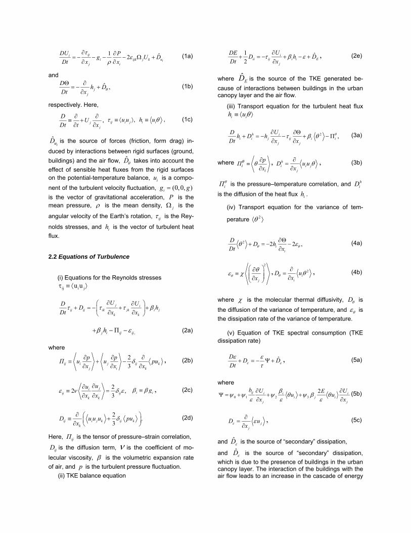
Figure 3 shows the vertical profile of the normal-ized local friction velocity obtained via the numerical model. In this figure, observational data are depicted as functions of the normalized coordinate Z/ZH, where ZH is the average height of a building in the urban canopy layer. All data are normalized by the maxi-mum local friction velocity . These data show a maximum at a height approximately equal to twice the average height of a building and substantially smaller values inside the urban canopy layer. The area below the maximum is usually referred to as the roughness sublayer. Since there is no reliable information about the time of measurements and meteorological condi-tions for the data obtained by different authors, the calculated values of the friction velocity were aver-aged over all calculations during their 24-h cycle. As is seen in the figure, the calculated friction velocity increases with height from the underlying surface, reaches a maximum value at the height larger than

*maxu

HZ , then decreases slightly with increasing height. Such a behavior is consistent with the Monin–Oboukhov similarity theory of the surface layer (the layer of constant flow). The small decrease with in-creasing height is in good agreement with observa-tional data (Oikawa and Meng, 1995; Feigenwinter, 1999). The extensive data set of measurements in the cities is presented in review of Roth (2000) for the ratio of the local friction velocity to the mean ve-

locity of horizontal wind (six groups of data). The cal-culated profile of (squares in Fig. 4) has a maximum near the top of the building and then de-creases with increasing height, reaching a value close to 0.1 at a height of about a fourfold average height of the building. The profiles calculated for two values of the geostrophic wind (3 and 5 m/s) are in good agreement with observational data.

*u

* /u U

The simulated results presented in these two fig-ures show that the modified model of turbulence for the ABL and a more realistic model of urban rough-ness (Fig. 2b) are able to reproduce the vertical pro-files of both the turbulent momentum flux and the mean velocity of horizontal wind that are consistent with observational data.

u* / U

Z/Z

H

0 0.05 0.1 0.15 0.2 0.25 0.3 0.350

1

2

3

4

5

6

7

1 2

Real scale datafrom Roth (2000)

Computation:UG=3ms-1

UG=5ms-1

Figure 4. Vertical profiles of the ratio of the lo-cal friction velocity to the average horizon-tal wind velocity at the center of the urbanized area. The symbols correspond to the data of different authors’ measurements presented in Fig. 1b of (Roth, 2000). The other notation is the same as in Fig. 3.

*u

Z, km

1

0 1 2 3 4 5

0.05

0.1

0.15

0.2

0.25

0.3

2

0Θ K

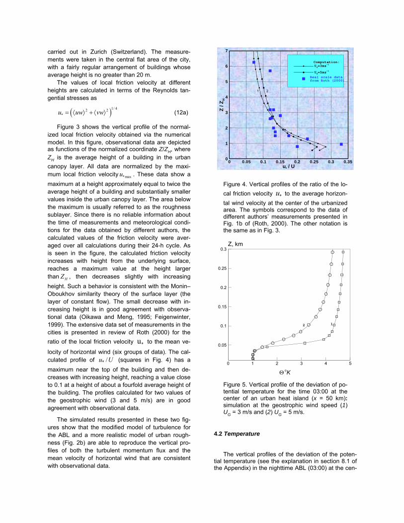
Figure 5. Vertical profile of the deviation of po-tential temperature for the time 03:00 at the center of an urban heat island (x = 50 km): simulation at the geostrophic wind speed (1) UG = 3 m/s and (2) UG = 5 m/s.

4.2 Temperature

The vertical profiles of the deviation of the poten-tial temperature (see the explanation in section 8.1 of the Appendix) in the nighttime ABL (03:00) at the cen-

ter of an urbanized surface are calculated with the modified three-parameter model of turbulence for the ABL and are shown in Fig. 5 for low (3 m/s) and high (5 m/s) geostrophic wind speeds. Comparison with the results of measurements over Sapporo (Japan) exhibits good qualitative agreement with a measured profile of potential temperature (see profile 18U in Fig. 5a of Uno and Wakamatsu (1992) both inside and outside the urban canopy layer. The measurements of series 18U recorded a raised inversion with its base at a height no greater than 60 m. The existence of the elevated nighttime inversion is similar to that over the convective mixed layer; however, the nature of at-mospheric stability and turbulence inside the corre-sponding layers is different (Uno and Wakamatsu, 1992).

4.3. Turbulent Structure of Urban Atmospheric Boundary Layer

The structure of turbulence in the boundary layer over an urbanized surface is represented by the pro-files of TKE (Fig. 6), standard deviation of the vertical velocity (Fig. 7), and vertical turbulent heat flux (Fig. 8).

E / (u* max)2

Z/Z

H

0 1 2 3 4 5 6 7 80

1

2

3

4

5

1

4

2

3

Figure 6. Vertical profiles of the turbulent ki-netic energy at the center of the urbanized area that are normalized by the maximum value of the friction velocity squared: simula-tion at the geostrophic wind speed (solid lines) UG = 3 m/s and (dashed lines) UG = 5 m/s; re-sults of simulation for the time (1, 3) 12:00 and (2, 4) 24:00. Different symbols show meas-urement data: - (Rotach, 1991; 1993; 1995),

- (Oikawa and Meng, 1995), - (Feigenwin-ter, 1999), and - (Louka et al., 2000).

(<w2>)1/2/u*max

Z/Z

H

0.5 1 1.5 2 2.50

1

2

3

4

5

6

7

12

Figure 7. Vertical profile of the standard devia-tion for the vertical velocity at the center of the urbanized area: simulation at the geostrophic wind speed (1) UG = 3 m/s and (2) UG = 5 m/s. The symbols denote the measurement data (see, Roth, 2000).

Z, km

-0.015 -0.01 -0.005 0 0.005 0.01 0.015

0.05

0.1

0.15

0.2

0.25

0.3

12

⟩θ⟨w ( K0 m s-1)

Figure 8. Vertical turbulent heat flux at the cen-ter of the urbanized area for the time 03:00: simulation at the geostrophic wind speeds (1) UG = 3 m/s and (2) UG = 5 m/s.

Figure 6 shows the TKE vertical profiles normalized by the maximum friction velocity squared (see the definition in Section 4.1) at the center of an urbanized surface that are simulated for the (instantaneous) moments 12:00 and 24:00. The same figure presents some results of different databases of urban meas-urements (Rotach, 1991; 1993; 1995; Oikawa and Meng, 1995; Feigenwinter, 1999; Louka et al., 2000). These measurements are carried out for different

morphologies of urban roughness and under different meteorological conditions. The scatter of the meas-urement data is significant. Some data show a de-crease in the TKE in the canopy layer relative to its value above this layer in accordance with a large amount of data of measurements and simulations in the vegetation layer (Raupach et al., 1991). With cer-tain restrictions, these data can be considered similar to those obtained over the canopy layer (buildings) characterized by another effect of mechanical factors on the flow. The numerical results obtained in this study have a correct behavior in the canopy layer and above it. In any case, it is believed that the effect of TKE decreasing in the canopy layer is reproduced by the model. Note that the three-parameter model of thermally stratified turbulence yields satisfactory re-sults when data obtained under controlled conditions of a laboratory experiment are used (Kurbatskii, 2001; Kurbatskii and Kurbatskaya, 2001) and adequately describes the TKE behavior for different states of at-mospheric stability. The day-night difference of behav-iour of the TKE is difficult to explain because of a wide scatter of the observational data. The profile of standard deviation of the vertical veloc-ity *max/W uσ is shown by the solid line in Fig. 7 along with the data of measurements (eight data groups) presented in review of Roth (2000; fig. 2f).These data are depicted by the symbols (blue squares).

From the considerations stated in Section 4.1, Fig. 7 shows the modeling results averaged over all calcu-lations during their 24-h cycle. We note that the calcu-lated profiles are close to the center of the range of data scatter. The normalization is performed with the friction velocity averaged over all values calculated for 24 h (by the same reasoning as in Section 4.1). Thus, it may be inferred that, for this structure characteristic of the turbulence field, this ABL model gives results that are in satisfactory agreement with observational data.

The calculated profiles of vertical heat flux (Fig. 8) are qualitatively consistent with the profiles measured over Sapporo (Uno and Wakamatsu. 1992). Although the measurement data are characterized by a rather wide scatter, a marked minimum near the inversion boundary is present in the data of Uno and Waka-matsu (1992) in Fig. 7 for the chosen time (03:00). The flux gradient changes sign, thus pointing to the heat flux directed downward from the base of the ele-vated inversion layer. 4.4. Effect of an Urbanized Surface on Mesoscale Flow

The results of the previous section relate primarily to the behavior of flow near an urbanized surface and

show that the modified three-parameter model is able to reproduce some important characteristics recorded during observations in cities. This section analyzes the results associated with the effect of urban roughness on the global structure of the ABL to find out to what extent the results obtained with the proposed ABL model are in agreement with observational data and other calculations. Situations with both a weak geostrophic wind, when thermal-stratification effects are of greatest importance and a strong geostrophic wind are discussed.

The numerical results presented in Figs. 3–9 are obtained for two values of the geostrophic wind speed: UG = 3 m/s and UG = 5 m/s. On the one hand, such wind-speed values are chosen for a qualitative comparison of the results of this test with the results of the same test of Martilli et al.(2002), where the one-parameter turbulence model is used to calculate all turbulent momentum and heat fluxes with an isotropic effective coefficient of turbulent exchange and with the initiation of an urban heat island via determination of the temperature of the underlying surface from the solution of the equation of heat balance at the surface with consideration for all heat fluxes at the surface, including radiative fluxes.

The results of this test are obtained from a physi-cally more correct calculation of all turbulent fluxes (of momentum and heat) and with the initiation of an ur-ban heat island through specification of the tempera-ture difference between the city and its environs. On the other hand, a small difference between the values of the geostrophic wind speed (3 and 5 m/s) can pro-vide a certain idea of the sensitivity of the improved model for an urban ABL to small variations in the geostrophic wind speed UG (in particular, for such an integral characteristic as the ABL height above the city). 4.4.1. Daytime ABL. The calculated vertical section of potential temperature at noon (12:00 of a diurnal cycle of modeling the evolution of the urban ABL) in Fig. 9a clearly shows a vertical heated-air column developing over the city and being advected downwind by the synoptic flow: sensible heat fluxes in the city are greater than those in its environs (rural area). This effect, along with the strong turbulence generated by the city’s rough structure, increases the height of the boundary layer, as is shown in the figure by the dashed line, from about 800 m in the city’s environs to 1.5 km over the city. (The ABL height is defined (Mar-tilli et al., 2002) by the height of the layer of the model’s computational grid at which the TKE is smaller than or equal to 0.01 m

2 s

–2.) Such an in-

creased boundary layer over the city as compared to that in the environs was observed, for example, by Spanton et al. (1988). The horizontal wind field in Fig. 9b shows low wind speeds near the surface of the city.

3.0

3.5

3.53.5

4.0

4.0

4.54.55.0

5.55.56.06.0

6.56.57.07.0

7.57.58.08.0

8.58.5

4.03.5

4.5

4.0

3.5

6.5

X, KM

Z,K

M

20 40 60 80 100 120

0.5

1

1.5

2

2.5a)

0

2 .25

2.75

2.75

2.753.25

3.25

3.753.754 .254.75

2.752.25

2.25

3.75

2.25

3.25

X,KM

Z,K

M

20 40 60 80 100 120

0.5

1

1.5

2

2.5

0

b)

3.0

3.0

3.5

4.0

4.0

4.0

4.5

4.54.5

5.05.05.55.5

6.06.06.56.5

7.07.07.57.57.5

8.08.08.58.5

3.5 3.53.0

3.0

5.0

6.56.0

8.5

4.0

4.0

3.0

3.5

5.0

3.5

X, KM

Z,K

M

20 40 60 80 100 120

0.5

1

1.5

2

2.5

0

c)

1.8 2.32.8

3.8 3.8

2 8

4.8

4.3

4.8

4.3

4.8

4.8 5.3

5.3

5.34.8

4.8

5.3

5.3

5.8

4.8

4.8

3.8

X,KM

Z,K

M

20 40 60 80 100 120

0.5

1

1.5

2

2.5

0

d)

1.3

1.3

1.31.8

1.8

1.8

2.3

2.32 .3

2.8

2.8

2.82.8

2.8

2.8

3.3

3.3

3.3

3.33.3

3.33. 3

3.8

3.84.3

1.32.3

X,KM

Z,K

M

20 40 60 80 100 120

0.1

0.2

0.3

0.4

0.5

0

f)5.0

4.54.5

4.0 4.03.53.5

4.5

4.0

4.5

X, KM

Z,K

M

20 40 60 80 100 120

0.1

0.2

0.3

0.4

0.5

0

e)

Figure 9. Calculated (a, c, e) vertical sections of the deviation of potential temperature (K) and (b, d, f) horizontal wind speed (m/s) for the time (a, b, c, d) 12:00 and (e, f) 24:00 at the geostrophic wind speed (a, b, e, f) 3 and (c, d) 5 m/s. On the sections of potential temperature, the dashed line shows the ABL height, which is determined as the level at which the TKE is smaller than 0.01 m2/s2. The segment of the heavy line with the abscissa from 45 to 55 km marks the location of the urbanized area (city).

2.25

2.25

2.25

2.75

2.75

2.75

2.75

3.25

3.25

3.25

3.75

3.754.25

4.75

2.25

4.25

2.75

2.25

4.75

X, km

Z,km

20 40 60 80 100 120

0.5

1

1.5

2( a )

2.25

2.25

2.25

2.75

2.75

2.75

2.75

2.75

3.25

3.25 3.25

3.75

3.75

3.75

2.752.25

2.75

2.25

4.25

2.25

X, km

Z,km

20 40 60 80 100 1200

0.5

1

1.5

2( b )

Figure 10. Calculated vertical sections of horizontal wind speed (m/s) for the time 12:00: (a) - simulation with the classical MOST approach and (b) - simulation with the parameterization of urban roughness. The thick line on the abscissa between 45 km and 55 km indicates the location of the urbanized area (city).

It possible to make some quantitative estimation of the wind speed changes above city influenced by the mechanical (urban roughness) and thermal (the urban heat island effect) inhomogeneity of the urbanized area. Fig. 10(a) shows results of the simulation with only the classical MOST approach. The simulation with the parameterization of the urban roughness in Fig. 10(b) is represented. It follows from these figures that the urban roughness reduces the wind speed above the city by about 24 percent, as compared with the classical MOST approach. Thus, the increase in wind speed above the city most is likely connected with the urban heat island effect. A similar modifica-tion of the wind speed above the city was probably simulated (for example, Martilli et al., 2002).

The influence of this effect on the structure of the

ABL with usual roughness (Fig. 2a) and with a heat island during the implementation of the same simple two-dimensional test is shown by Kurbatskii (2005). Other things being equal, the height of the boundary layer turns out to be greater in the presence of longi-tudinal turbulent diffusion of heat than in its absence. Indeed, the calculated results shown in Fig.11 allow estimating the effect of the longitudinal turbulent heat diffusion on the boundary layer characteristics. It is seen from Fig.11 that the height of the boundary layer above city (marked by the dashed line) in the pres-ence of diffusion is higher than in its absence. The longitudinal diffusion transports the heat into the col-umn of the heated air above the city (heat spot), which increases the TKE generation due to the fluctu-ating buoyancy force and favors the increase of the PBL height.

a b

Figure 11. Vertical sections of the deviations of the potential temperature, calculated taking into account (a) and ne-glecting (b) the longitudinal turbulent heat diffusion at 12:00 a.m. (UG=5 m/s).

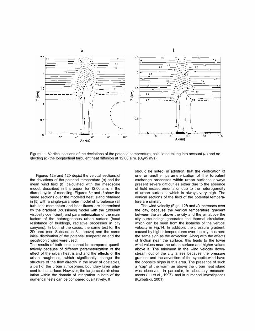
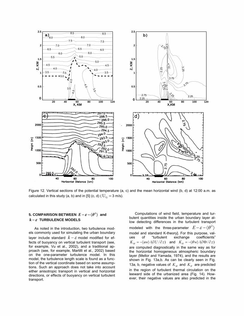
Figures 12a and 12b depict the vertical sections of the deviations of the potential temperature (a) and the mean wind field (b) calculated with the mesoscale model, described in this paper, for 12:00 a.m. in the diurnal cycle of modeling. Figures 3c and d show the same sections over the modeled heat island obtained in [5] with a single-parameter model of turbulence (all turbulent momentum and heat fluxes are determined by the gradient Boussinesq model with the turbulent viscosity coefficient) and parameterization of the main factors of the heterogeneous urban surface (head resistance of buildings, radiative processes in city canyons). In both of the cases, the same test for the 2D area (see Subsection 3.1 above) and the same initial distribution of the potential temperature and the geostrophic wind were used. The results of both tests cannot be compared quanti-tatively because of different parameterization of the effect of the urban heat island and the effects of the urban roughness, which significantly change the structure of the flow directly in the layer of obstacles, a part of the urban atmospheric boundary layer adja-cent to the surface. However, the large-scale air circu-lation within the domain of integration in both of the numerical tests can be compared qualitatively. It

should be noted, in addition, that the verification of one or another parameterization of the turbulent exchange processes within urban surfaces always present severe difficulties either due to the absence of field measurements or due to the heterogeneity of urban surfaces, which is always very high. The vertical sections of the field of the potential tempera-ture are similar.

The wind velocity (Figs. 12b and d) increases over the city, because the vertical temperature gradient between the air above the city and the air above the city surroundings generates the thermal circulation, which can be seen from the isotachs of the vertical velocity in Fig.14. In addition, the pressure gradient, caused by higher temperatures over the city, has here the same sign as the advection. Along with the effects of friction near the surface, this leads to the lower wind values near the urban surface and higher values above it. The minimum in the wind velocity down-stream out of the city arises because the pressure gradient and the advection of the synoptic wind have the opposite signs in this area. The presence of such a "cap" of the warm air above the urban heat island was observed, in particular, in laboratory measure-ments (Lu et al., 1997) and in numerical investigations (Kurbatskii, 2001).

3.0

3.5

3.53.5

4.0

4.0

4.54.55.0

5.55.56.06.0

6.56.57.07.0

7.57.58.08.0

8.58.5

4.03.5

4.5

4.0

3.5

6.5

X, KM

Z,K

M

20 40 60 80 100 120

0.5

1

1.5

2

2.5a)

0

2 .25

2.7 5

2.75

2.75

3.25

3.25

3.753.754.2 54.75

2.752.25

2.25

3.75

2.25

3.25

X,KM

Z,K

M

20 40 60 80 100 120

0.5

1

1.5

2

2.5

0

b)

Figure 12. Vertical sections of the potential temperature (a, c) and the mean horizontal wind (b, d) at 12:00 a.m. as calculated in this study (a, b) and in [5] (c, d) ( GU = 3 m/s). 5. COMPARISON BETWEEN 2ε θ− − ⟨ ⟩E and

ε−k TURBULENCE MODELS

As noted in the introduction, two turbulence mod-els commonly used for simulating the urban boundary layer include standard −k ε model modified for ef-fects of buoyancy on vertical turbulent transport (see, for example, Vu et al., 2002), and a traditional ap-proach (see, for example, Martilli et al., 2002) based on the one-parameter turbulence model. In this model, the turbulence length scale is found as a func-tion of the vertical coordinate based on some assump-tions. Such an approach does not take into account either anisotropic transport in vertical and horizontal directions, or effects of buoyancy on vertical turbulent transport.

Computations of wind field, temperature and tur-

bulent quantities inside the urban boundary layer al-low detecting differences in the turbulent transport

modeled with the three-parameter 2E ε θ− − ⟨ ⟩ model and standard K-theory]. For this purpose, val-ues of “turbulent exchange coefficients”

/( / )MK uw U z= −⟨ ⟩ ∂ ∂ and /( / )HK w zθ= −⟨ ⟩ ∂Θ ∂ are computed diagnostically in the same way as for the horizontal homogeneous atmospheric boundary layer (Mellor and Yamada, 1974), and the results are shown in Fig. 13a,b. As can be clearly seen in Fig. 13a, b, negative values of MK and HK are predicted in the region of turbulent thermal circulation on the leeward side of the urbanized area (Fig. 14). How-ever, their negative values are also predicted in the

lower urban boundary layer part for MK and upper

urban boundary layer part for HK .

Regions of negative values of MK and HK ex-plicitly indicate non-local character of the turbulent transport which can not be described using simple one- or two-parameter turbulence models. In these two models, it is difficult to correctly account for ef-

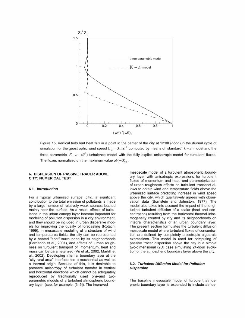
fects of buoyancy on the turbulent transport of mo-mentum, mass and heat. For example, figure 15 shows that the ‘standard’ model underpredicts values of the vertical turbulent heat flux when com-pared with the

k − ε

2E ε θ− − ⟨ ⟩ model and fully explicit anisotropic model for turbulent fluxes of momentum, mass and heat.

a b

80.040.0 -80.

0

-80.0

X,km

Z,

km

45 50 550

0.5

1

1.5

2

C I T Y

'Negative' turbulent viscosity12:00

80.0

80.0

-80.0

80.0

-80.0

-80.0-80.0

X, km

Z,km

45 50 55

0.5

1

1.5

2

C I T Y

' Negative' turbulent thermal diffusivity12:00

Figure 13. Momentum ( ) and heat (a b ) turbulent exchange coefficients for Urban simulation at noon. Results

are for the case with geostrophic wind. 13ms−

0.8

0.8

0.8

2.8

2 .8

0.4

-0.4

-0.4

-0.4

-0.3

-0.3-0.5

-0.5

-0.3

X , km

Z,k

m

40 45 50 55 60 65

0.5

1

1.5

2

2.5

0

Figure 14. Velocity vectors and isotachs ( 1ms− ) for vertical velocity at 12:00 (noon) in the diurnal cycle of

simulation for the geostrophic wind speed 1GU 3ms−= .

iz / z

0 0.2 0.4 0.6 0.8 10

0.5

1

1.5

three-parametric model

Κ − ε model

0w / w⟨ θ⟩ ⟨ θ⟩

Figure 15. Vertical turbulent heat flux in a point in the center of the city at 12:00 (noon) in the diurnal cycle of simulation for the geostrophic wind speed 1

GU 3ms−= computed by means of ‘standard’ k ε− model and the

three-parametric 2E ε θ− − ⟨ ⟩ turbulence model with the fully explicit anisotropic model for turbulent fluxes. The fluxes normalized on the maximum value of 0w⟨ θ⟩ .

6. DISPERSION OF PASSIVE TRACER ABOVE CITY: NUMERICAL TEST

6.1. Introduction For a typical urbanized surface (city), a significant contribution to the total emission of pollutants is made by a large number of relatively weak sources located mainly near the surface. As a result, effects of turbu-lence in the urban canopy layer become important for modeling of pollution dispersion in a city environment, and they should be included in urban dispersive mod-els for improving the quality of forecasting (Rotach, 1999). In mesoscale modeling of a structure of wind and temperatures fields, the city can be represented by a heated "spot" surrounded by its neighborhoods (Fernando et al., 2001), and effects of urban rough-ness on turbulent transport of momentum, heat and mass can be parameterized (Vu et al., 2002; Martilli et al., 2002). Developing internal boundary layer at the “city-rural area" interface has a mechanical as well as a thermal origin. Because of this, it is desirable to preserve anisotropy of turbulent transfer in vertical and horizontal directions which cannot be adequately reproduced by traditionally used one-and two-parametric models of a turbulent atmospheric bound-ary layer (see, for example, [3, 5]). The improved

mesoscale model of a turbulent atmospheric bound-ary layer with anisotropic expressions for turbulent fluxes of momentum and heat, and parameterization of urban roughness effects on turbulent transport al-lows to obtain wind and temperature fields above the urbanized surface predicting increase in wind speed above the city, which qualitatively agrees with obser-vation data (Bornstein and Johnston, 1977). The model also takes into account the impact of the longi-tudinal turbulent diffusion of a scalar (heat and con-centration) resulting from the horizontal thermal inho-mogeneity created by city and its neighborhoods on integral characteristics of an urban boundary layer. The present section formulates the turbulent diffusion mesoscale model where turbulent fluxes of concentra-tion are defined by completely anisotropic algebraic expressions. This model is used for computing of passive tracer dispersion above the city in a simple two-dimensional (2D) case simulating 24-hour evolu-tion of the atmospheric boundary layer above the city. 6.2. Turbulent Diffusion Model for Pollution Dispersion The baseline mesoscale model of turbulent atmos-pheric boundary layer is expanded to include atmos-

pheric dispersion of a passive contaminant by adding equations for mean concentration , turbulent

contaminant flux and correlation

( , )iC x t

j if u c≡< > θ< >c . Numerical results from validations of differential and algebraic models for turbulent concentration fluxes used in modeling of passive tracer dispersion above an urban heat island under conditions of night-time atmospheric boundary layer (weak wind, stable strati-fied atmosphere) have shown (Raupach et al., 1991) that the algebraic model for turbulent concentration fluxes provides acceptable in accuracy results. Such a model is formulated by simplifying closed differential transport equation for the turbulent scalar flux iu c⟨ ⟩ under the same local-equilibrium turbulence assump-tion applied in section 2. 3 for simplification of equa-tions for turbulent momentum (Reynolds stresses) and heat flux.

1α ε⎧< > ∂ < >∂

− < >⎨∂ ⎩∂∂

− < > − < > −∂ ∂

is k l

k

ii j j

j j

D u c u cE u uDt x x

UCu u u cx x

⎫=⎬∂ ⎭

i

l

3α β θ β θ+ < > − <c i ig c g c > −

1 2εα α

∂− < > + < >

∂i

c i c jj

Uu c u c

E x. (13a)

This approach assumes that the left hand side of (13a) can be neglected and the following algebraic equation for is obtained, j if u c≡ ⟨ ⟩

23

δε

∂⋅ = − + +

∂ij j ij ijj

E CA f ( b E )x

2 31 α β δ θε

+ − ⟨ ⟩C iE( ) g c (13b)

where ij i j ijb u u (2 / 3)E= ⟨ ⟩ − δ is the traceless Rey-

nolds stress tensor. The closed prognostic equation of (13c) for correlation

(Enger, 1986) is, c⟨ θ⟩

θθ Θθ⟨ ⟩

⟨ ⟩ ∂ ∂− = −⟨ ⟩ − ⟨ ⟩

∂ ∂c j j −j j

D c CDiff u u cDt x x

3εα θ− ⟨ ⟩C c ,E

(13c)

where is the turbulent transfer term, also re-duced under the weak-equilibrium turbulence ap-proach to the algebraic equation,

cDiff⟨ θ⟩

3

1 Θθ θα ε

⎛ ⎞∂⟨ ⟩ = − ⟨ ⟩ + ⟨ ⟩⎜ ⎟⎜ ⎟∂ ∂⎝ ⎠

j jC j

E Cc u c u ∂

jx x (13d)

Substituting (13d) into (13b) yields the algebraic equa-tion for flux concentration jf

23

δε

⋅ = − + +ij j ij ijEA f ( b E )

23

3

1 αβ δ

α ε− ∂

+∂

Ci j

C j

( ) E Cg h x

(13e)

where

1α δε∂

= + +∂

iij C ij

j

UEAx

22

33

1 α Θβ δε α

− ∂⎛ ⎞+ ⎜ ⎟ ∂⎝ ⎠C

iC j

( )E gx

. (13f)

Anisotropic expressions for vertical and hori-

zontal

wc⟨ ⟩uc⟨ ⟩ turbulent fluxes of concentration are

derived by means of symbolical algebra from (13e) in following form,

21 1

1 α α λ θε

∂⎛ ⎞⎡ ⎤−⟨ ⟩ = ⟨ ⟩ + ⟨ ⟩ +⎜ ⎟⎣ ⎦ ∂⎝ ⎠*

CE Cwc w w

D z

1 11 α α λ θ

ε∂⎛ ⎞⎡ ⎤+ ⟨ ⟩ + ⟨ ⟩⎜ ⎟⎣ ⎦ ∂⎝ ⎠

*C

E Cuw uD x

,(13g)

22

1 ( [ (∂−⟨ ⟩ = ⟨ ⟩λ + ⟨ ⟩ +

ε ε ∂E E Uuc u uw

D z

*1 )]) ∂+α λ ⟨ θ⟩ +

∂Cux 2

1 ( [⟨ ⟩λ +εE uw

D

( )2 *1 ])∂ ∂

+ ⟨ ⟩ + α λ ⟨ θ⟩ε ∂ ∂E U Cw w

z z. (13h)

In these expressions, *

2C 3C(1 ) /α = −α α ,

1 ( / )λ = β εg E ,

*2 1 3

∂ ∂Θλ = α + +α λ

ε ∂ ∂CE W

z z,

23 ( / )λ = β εg E .

In From (13g) and (13h) the equation for mean con-centration

∂ ∂ ∂+ ⋅ + ⋅ =

∂ ∂ ∂C C U C Wt x z

∂ ∂

− ⟨ ⟩ − ⟨ ⟩∂ ∂

wc ucz x

(13i)

is reduced to the closed form after neglecting molecu-lar diffusion at higher Reynolds numbers. The numeri-cal constants of diffusion models (13g) – (13i) are:

1С 3С 3,28α = α = , 2С 0,4α = .

6.3. Results of Numerical Modeling of Passive Tracer Dispersion above City

The computed tracer concentration in the city centre at the lowest modeled level during 48-hour cycle of simulating the urban boundary layer evolution is pre-sented on fig. 16. As expected, the concentrations are higher during the night than during the day, because the nocturnal boundary layer is much thinner than the

diurnal one. It should be noted here that the overpre-diction of primary pollutants during the night in urban areas, as compared to the measurements, is fairly common for Eulerian photochemical models, espe-cially under low wind conditions (Moussiopoulos et al., 1997). This problem can be linked to an inappropriate reproduction of the nocturnal urban heat island.

8 16 24 32 40 48 560

1000

2000

C

Figure 16. Time evolution of passive tracer surface concentration in the centre of the urban area as computed by the three-parameter turbulence model. Results are for the case with the geostrophic wind 3 m/s. GU =

X , km

C/C

max

20 40 60 80 100 1200

0.25

0.5

0.75

1

07:00 (first day)13:00 (second day)

Figure 17. Passive tracer concentration. At the lowest level at 13:00 a.m. of the second day. The city is located be-tween 45 km and 55 km. Results are for the case with the geostrophic wind GU = 3 m/s.

Thus, influence of the urban surface on the day time pollutant concentration away from the city is clearly shown. This result is in qualitative agreement with calculations (Martilli et al., 2002)]. The above-noted behavior of concentration in a vicinity of city’s leeward side is caused by the nature of the thermal circulation moved by advection downwind to the leeward side (see also a Figure 14 showing the isotachs of vertical wind speed (arrows show the average wind vector field).

A method of simulating pollutant dispersion in mesoscale atmospheric models is presented in this section. Influence of the urban roughness (buildings) is not explicitly resolved, but their effects on the grid-averaged variables are parameterized. In Eulerian diffusion models, turbulent fluxes of concentration are computed from completely explicit algebraic expres-sions taking into account the anisotropy of transfer in vertical and horizontal directions. Numerical results of passive tracer dispersion emitted at ground level in the centre of the urban area correctly reflect behavior of concentration near the surface during the 24-hour evolution of the urban boundary layer. Impact of the city on day time concentration of pollution away from it during the second day is correctly predicted by the numerical model. 7. CONCLUSIONS

A three-parameter mesoscale model of explicit

anisotropic turbulent fluxes of momentum and heat has been developed in this paper for modeling at-mospheric flows over an inhomogeneous underlying surface. An important property of the model lies in the improvement of estimating the processes of transfer in the vertical and horizontal directions under different stratification conditions, which are usually observed in an urban boundary layer. A simple two-dimensional numerical test on the influence of mechanical factors (urban roughness) and thermal factors (effect of an urban heat island) on a global structure of the atmos-pheric boundary layer has been implemented. This test has shown that the results of numerical simulation are in good qualitative and quantitative agreement with the data of field measurements. The model is able to reproduce turbulent processes within the ur-ban canopy layer and above it with satisfactory accu-racy. The formulated model of turbulent fluxes with closure level 3.0 can be potentially used to model the atmospheric boundary layer within the “urban” scale and “mesoscale.” The improvement of the model re-quires a more accurate calculation of heating proc-esses in the urban canopy layer, and this modification of the model is regarded as the aim of our further study. Note that the description of a detailed pattern of urban climate requires measurement data on turbu-lent quantities within the urban canopy layer. Such data allow a more accurate specification of the de-sired functions of the three-parameter model at the lower boundary near the surface (at the first computa-

tion level), because the use of the approximations of constant fluxes in the surface layer that are based on the Monin–Oboukhov theory does not allow an ade-quate (to the data of field measurements; see, for example, Rotach, 1993) reproduction of the vertical structure of turbulent fields in the urban canopy layer (from the level of the urban street canyon to heights of 50–100 m). It is clear that a realistic modeling of the dispersion of urban pollutants requires an accurate knowledge of meteorological parameters for this re-gion of the urban ABL, where the pollutants are emit-ted and where people live. An efficient use of this model for the turbulent ABL requires the specification (from measurement data) of “input” parameters such as the vertical distributions of the three base functions of the model, E, ε, and 2θ⟨ ⟩ (for example, in the morning hours for a stably stratified ABL). Testing the potentials of the RANS turbulence model for an urban ABL requires the measurement data on the distribu-tions of a number of quantities, such as the variance of the vertical component of turbulent velocity and the boundaries of surface and raised inversions (including those under the conditions of weakened ABL turbu-lence in the night and early-morning hours, measure-ment data on vertical distributions of temperature, turbulent heat flux, TKE, and other parameters). 8. APPENDIX

The Appendix presents the governing system of equations of a turbulent horizontally inhomogeneous thermally stratified ABL for the two-dimensional test under study. Explicit analytic expressions are given for the turbulent momentum and heat fluxes, and nu-merical values are presented for the constants of the modified three-parameter model of turbulence. De-tailed expressions are presented for the parameteriza-tion of the effects of urbanized-surface roughness.

8.1. Governing System of Equations for the Tur-bulent ABL

For flows in a planetary boundary layer, some ap-proximations can be used in the governing equations. In (1a), the rotation term can be approximated with the expression

32ε Ω ε− =ijk j k c ij jU f U

where the axes x, y, and z are directed eastward, north-ward, and upward, respectively, and fc = 2Ωsinφ is the Coriolis parameter with the angular velocity of the Earth’s rotation Ω and latitude φ. The buoyancy effects are taken into account in the Boussinesq ap-proximation, and, for a two-dimensional flow, the sys-tem of equations (1a) and (1b) is written as

0,+ =x zU W (14a)

1 ˆ ,ρ

+ + = − − + +t x z x zU UU WU P wu fV Du (14b)

ˆ ,+ + = − − +t x z zV UV WV wv fU Dv (14c)

0

1 ˆ ,βρ

+ + = − − + Θt x z z zW UW WW P ww g (14d)

ˆ ˆ ˆ ˆ .θθ θΘ + Θ + Θ = − − +t x z x zU W u w D (14e)

The dependent variables in (14a)–(14e) are the mean (time averaged) flow velocitiesU ,V and W in the directions of the x , y and axes, respectively, the mean pressure , and the mean departure of poten-tial temperature from a reference temperature T

zPΘ 0.

The parametric quantities in (14a)–(14e) include the volumetric expansion rate of air β (3.53 ×10

–3 K

–1),

the mean air density 0ρ . The lower case letters de-note turbulent fluctuations of the corresponding quan-tities. The Reynolds turbulent stresses τ ij and the

turbulent heat flux vector jh in equations (14a)–(14e)

requires modeling. Explicit algebraic models for the Reynolds stresses and the turbulent heat flux are for-mulated in the next section.

8.2. Algebraic Expressions for Turbulent Momentum and Heat Fluxes

From Eq. (9a) with consideration for 23

δ= ⟨ ⟩ −ij i j ijb u u E and from Eq. (10a) for the vec-

tor of turbulent heat flux θ= ⟨ ⟩i ih u the following im-

plicit system of equations for the turbulent momentum and heat fluxes is written in the boundary-layer ap-proximation:

22 2

2 (4 23 3

τ α α∂ ∂= − −

∂ ∂U Vu E uw vwz z

+

32 )α β θ+ g w , (15а)

22 2

2 (4 23 3

τ α α∂ ∂= − −

∂ ∂V Uv E vw uwz z

+

32

22 2

2 (2 23 3

τ α α∂ ∂= + +

∂ ∂U Vw E uw vwz z

+

34 )α β θ+ g w , (15c)

22 32

2τ α α τβ θ∂

= − +∂Uuw w g uz

, (15d)

22 32

2τ α α τβ θ∂

= − +∂Vvw w g vz

, (15e)

2τα ∂ ∂⎛= − +⎜ ∂ ∂⎝ ⎠

V Uuv uw vwz z

⎞⎟ , (15f)

45

τθ α θα

∂Θ ∂⎛ ⎞= − +⎜ ⎟∂ ∂⎝ ⎠

Uu uwz z

w , (15g)

45

τθ α θα

∂Θ ∂⎛ ⎞= − +⎜ ⎟∂ ∂⎝ ⎠

Vv vwz z

w , (15h)

24

5

τθ αα

∂Θ⎛ ⎞= − −⎜ ⎟∂⎝ ⎠w w g

z2β θ . (15i)

Equations (15a)–(15i) were solved via symbol al-gebra. Below, we present expressions for those turbu-lent momentum and heat fluxes that were used in a numerical test to solve system of equations (14a) – (14e):

( ), ∂ ∂⎛= − ⎜ , ⎞⎟∂ ∂⎝ ⎠

MU Vuw vw Kz z

, (16a)

θ γ∂Θ= − +

∂Hw Kz c , (16b)

τ=M MK E S , τ=H HK E S , (16c)

( )0 1 2 31 1⎡ ⎤= + − +⎣ ⎦M HS s s G s s GD H

( )2

24 5 61 ( )

θτβ+ + Hs s s G g

E , (16d)

( 61

1 2 1 13 θ

)⎧ ⎫= +⎨ ⎬

⎩ ⎭HS

D c Hs G , (16e)

where

)α β θ+ g w , (15b)

2 22 6 5

1 21 (3

)γ α α τβ⎧ ⎫= + +⎨ ⎬⎩ ⎭

c M HG s G gD

θ . (16f)

is the countergradient term, which is absent in models with closure levels 2.0 and 2.5 (Cheng et al., 2002).

The quantities GH and GM are defined as

( )2τ≡HG N , , (16g) ( )2τ≡MG S

2 β ∂Θ=

∂N g

z,

2 22 ∂ ∂⎛ ⎞ ⎛ ⎞≡ +⎜ ⎟ ⎜ ⎟∂ ∂⎝ ⎠ ⎝ ⎠

U VSz z

and, for Eqs. (16a)−(16f), we have

21 2 3 41= + + + + +M H M H HD d G d G d G G d G

25 6⎡+ −⎣

⎤⎦H M H Hd G d G G G , (16h)

21 2

23α=d , 3

21

103 θ

α=d

c, 3

3 2 21

2 ( )3 θ

α5α α α= −d

c,

23

41

113 θ

α⎛ ⎞= ⎜ ⎟

⎝ ⎠d

c,

33

51

43 θ

α⎛ ⎞= ⎜ ⎟

⎝ ⎠d

c,

23

6 2 51

23 θ

αα α

⎛ ⎞= ⎜ ⎟

⎝ ⎠d

c,

0 223α=s , 3

12 1

1

θ

αα

⎛ ⎞= ⎜ ⎟

⎝ ⎠s

c, 2 2 5α α= −s ,

33 5

1θ

αα

⎛ ⎞= ⎜ ⎟

⎝ ⎠s

c, 4 3 5α α=s , 5 5

43 2α α= +s , 3

61θ

α=s

c,

25

1

1 θ

θα

−=

CC

. (16i)

The variance of the vertical turbulent velocity and the horizontal heat fluxes are determined from the ex-pressions

( ) ( )226 3 5

1 2 4 13 3

α α τβ θ= + +Hw E s G gD

2 ×

2 5 6112α α⎛ ⎞− +⎜

⎝ ⎠M HG s G ⎟ , (16j)

2 2 5 61

1 2 1 [ ( )3 θ

θ τ α α α= + + Hu E s GD c

+

5 ] α τ ∂ ∂Θ+ −

∂ ∂Uz z

2 25 5 2

1 2( ) 13

τ α τβ θ α α∂ ⎧ ⎛ ⎞− + +⎨ ⎜ ⎟∂ ⎝ ⎠⎩M

U g GD z

5 2 643

α α⎛ ⎞− +⎜ ⎟⎝ ⎠

Hs G

2 26 2 3 6 2

2 43 3

α α α ⎫+ − ⎬⎭

M H Hs G G s G2 , (16k)

2 2 5 61

1 2 1 [ ( )3 θ

θ τ α α α= + + Hv E s GD c

+

5 ] α τ ∂ ∂Θ∂ ∂Vz z

25

1 ( )τ α τβ θ∂− ×

∂V g

D z

25 2 5 2 6

2 4 (1 ) ( )3 3

α α α α+ + −M HG s +G

2 26 2 3 6 2

2 4 3 3

α α α+ − 2M Hs G G s GH . (16l)

8.3. Constants of the Three-Parameter Model of Turbulence

For the correlations with pressure fluctuations of

the dynamic turbulent field, the ‘standard’ models are used (Launder et al., 1975; Launder, 1996). These models were successfully applied in solving different problems; therefore, the values of the numerical coef-ficients in the model expressions for these correla-tions have been approved sufficiently well. These coefficients are presented (Launder, 1996) as the graphical dependence

(1 − c2)/c1 = 0,23. (16m)

For the relaxation coefficient in the model of the slow part of pressure-strain correlation (7b), the

value: c

(1)ijП

1 = 2.0 is taken from the commonly used range between 1.5 and 2.0. For c1 = 2.0, the numeri-cal value of the coefficient c2 found from (16m) is 0.54. When selecting the value of the coefficient c3 in the buoyancy terms in (7b), one can use the

solution of simple problems with allowance for buoy-ancy effects (Gibson and Launder, 1978; Lumley and Monsfield, 1984), c

3α ijB

3 = 0.776. Here, for this coefficient, the value 0.8 is taken, which corresponds to the value obtained by Cheng et al. (2002) via the renormaliza-tion-group technique. Numerical values of the coeffi-cients in the pressure-temperature correlation θ

iП in

(7c) are 1θc =3.28 and 2θc = 3θc =0.5. These values are calibrated during modeling of different turbulent

stratified flows, both homogeneous and inhomogene-ous (Kurbatskii, 2001; Sommer and So, 1995). We note that the numerical value coefficient calculated by Cheng et al. (2002) with use of the renormaliza-tion-group technique turned out to be 2.5. At the same time, it should be remembered that, for example, for the widely used

1c

ε−E model of turbulence, this tech-nique yields the values of the constants appearing in the ε - equation that are noticeably different from the values calibrated with the database of measurements and commonly used in computations. Numerical coef-ficients in the diffusion terms have the following val-ues: σ E =1.2, εσ =1.2, and θσ =0.6. In Eq. (5a) for

the TKE dissipation rate, we have 0ψ =3.8,

1ψ = 2ψ =2.4, and 3ψ =0.3 (Andren, 1990).

Note that the improved three-parameter anisot-ropic model for the turbulent ABL includes eight base constants ( , , ,1c 2c 3c 1c θ , 2c θ = 3c θ , 0ψ , 1ψ = 2ψ , 3ψ )

and three Prandtl numbers ( Eσ , εσ , θσ ), which enter into the models of processes of turbulent diffusion of the transfer equations for the functions ,E ,ε and

2θ⟨ ⟩ . The calibrated numerical values of these con-stants remain invariant during the solution of any problems of atmospheric turbulent flows with calcula-tion of not only the distributions of average hydro-thermodynamic fields but also the distributions of ani-sotropic turbulent momentum fluxes (normal and tan-gential turbulent stresses) and components of the vector of turbulent heat flux. The invariance of nu-merical values for the set of constants is a natural requirement that must be satisfied in any model that is constructed on the basis of the RANS (Reynolds Av-erage Navier–Stokes) approximation and that claims to obtain results consistent with the data of measure-ments and observations for a wide class of problems of stratified atmospheric flows. 8.4. Calculation of the Effects of Urban Rough-ness on a Flow in the ABL

In this numerical test, the urban heat island is modeled through specification of the temperature dif-ference between the urbanized surface and its vicini-ties and the time-dependent boundary condition for the temperature models a 24-h cycle of heating the Earth’s surface by the Sun. For this reason, the me-chanical factors are implemented by the parameteri-zation scheme completely, whereas the contribution to the balance of potential temperature is imple-mented only approximately (heating/cooling of the surfaces of buildings). The urban roughness effects are calculated according to the scheme of Martilli et al. (2002).

8.5. Boundary Conditions for System of Equa-tions of the ABL (14a)–(14e)

Following by Yamada and Mellor (1975)], one can find an expression for the ratio of the horizontal wind speeds at the first two computational nodes above the surface (z2 > z1 > 0). This expression represents the finite-difference boundary condition for the wind speed at the lower boundary and is written as

1 01 1

2 2 2 0

( / )( / )

ln z zU VU V ln z z

= = . (18а)

In our numerical test, the temperature measured at the ground surface is interpolated with dependence (11a). Therefore, according to Yamada and Mellor (1975), the boundary condition in a finite-difference form is also used for the temperature:

2 3ˆ ˆ ˆ (1 )g= + −θ θΘ Δ Θ Θ Δ , 2 0

3 0

ln /ln /

t

t

z zz z

=θΔ , (18b)

where z0t = 0.6z0 (z0 = 0.1 m in calculations).

In order to calculate turbulent fluxes near the sur-face, the MOST is used to relate vertical gradients in the surface layer and the empirical functionΦ , ob-tained from the data of the Kansas experiment, is taken from Andre et al. (1978). The boundary condi-tions are specified at the first (from the surface) com-putational node and have the form

2

1 *0 /E u c= μ , (18c)

31 *0 1( / 0, 41 1/ 0,41 )u z= −ε Φ L , (18d)

2/32 2

*04(1 8,3 ) , 04, 0

−⎧ − ≤⎪⟨ ⟩ = ⎨>⎪⎩

ζ ζθ θζ

, (18e)

*0 1ˆ ˆ( )

Pr gt

k z⎡ ⎤= − ×⎣ ⎦θ Θ Θ

[ ] 11 0 0 0ln( ) / ln( / )t otz z z z z −+ + −Φ , (18f)

1/ 4(1 15 ) , 01 5 , 0

−⎧ − ≤⎪= ⎨+ >⎪⎩

ζ ζΦζ ζ

/z L=ζ , 2*0 *0/(0,41 )L u g= β θ . (18g)

The frictional velocity and frictional temperature *0u

*0θ are computed using MOST and the no iterative scheme of Louis (1979).

Acknowledgments

This study was supported by the Russian Founda-tion for Basic Research (project No. 06-05-64002).

8.6 References Andre, J. C., De Moor, G., Lacarrere, P., Therry, G.

and du Vachat, R. 1978: Modeling the 24-hour Evolution of the Mean and Turbulent Structures of the Planetary Boundary Layer. J. Atmos. Sci. 35, 1861–1883.

Andren, A. 1990: Evaluation of a Turbulence Closure Scheme for Air-Pollution Applications. J. Appl. Me-teor. 29, 224–239.

⎯. 1990. A TKE-Dissipation Model for the Atmos-pheric Boundary Layer. Bound.-Layer Meteor. 56, 207–221.

Bornstein, R. and Johnson, D. S. 1977: Urban-Rural Wind Velocity Differences. Atmos. Environ. 11, 597–604.

Cheng, Y., Canuto, V. M. and Howard, A. M. 2002: An Improved Model for the Turbulent PBL. J. At-mos. Sci. 59, 1500–1565.

Enger L. 1986: A higher order closure model applied to dispersion in a convective PBL. Atmos. Environ. 20, 879-894.

Feigenwinter, C. 1999: The Vertical Structure of Tur-bulence above an Urban Canopy. PhD Thesis. University of Basel, 76 pp.

Fernando, H. J. S., Lee, S. M., Anderson, J., Princevac, M., Pardyak, E. and Grossman-Clarke, S. 2001: Urban Fluid Mechanics: Air Circulation and Contaminant Dispersion in Cites, Environ-mental Fluid Mech. 1, 107–164.

Gibson, M. M. and Launder, B. E. 1978: Ground Ef-fects on Pressure Fluctuation in the Atmospheric Boundary Layer. J. Fluid Mech. 86, 491–511.

Girimaji, S. S. and Balachandar, S. 1998: Analysis and Modeling of Buoyancy-Generated Turbulence Using Numerical Data. Int. J. Heat Mass Transfer 41, 915–929.

Kolmogorov, A. N. 1942: Equations of Turbulent Mo-tion of an Incompressible Fluid. Izv. Akad. Nauk SSSR, Ser. Fizicheskaya 6 (1–2), 56–58.

Kurbatskii, A. F. and Kazakov, A. V. 1999: Explicit Algebraic Model of Turbulent Heat Transfer for a Developed Flow in a Rotating Round Pipe. Ther-mophysics and Aeromechanics. 6, 231–240.

⎯, 2001: Computational Modeling of the Turbulent Penetrative Convection above the Urban Heat Is-land in a Stably Stratified Environment. J. Appl. Meteor. 40, 1748–1761.

⎯, and Kurbatskaya, L. I. 2001: Penetrative Turbu-lent Convection over a Heat Island in a Stably Stratified Environment. Izv. Akad. Nauk, Fiz. Atm. Okeana 37, 149–161 [Izv., Atmos. Ocean. Phys. 37, 135– 146.

⎯, Kurbatskii, A. F 2005: Numerical Investigation of Surface Heat Spot Effect on Atmospheric Bound

ary Layer Structure. Thermophysics and Aerome-chanics. 12, 39–58.

Launder, B. E. 1975: On the Effects of Gravitational Field on the Turbulent Transport of Heat and Mo-mentum. J. Fluid Mech. 67, 569–581.

⎯, Reece, G. and Rodi, W. 1975: Progress in the Development of a Reynolds-Stress Turbulent Clo-sure. J. Fluid Mech. 68, 537–566.

⎯, 1996. An Introduction to Single-Point Closure Methodology. In: Simulation and Modeling of Tur-bulent Flows. Oxford Univ. Press, New York, pp. 243-310.

Louis, J. F. 1979: A parametric model of vertical eddy fluxes in the atmosphere. Bound.-Layer Meteor. 17, 187-202.

Louka, P., Belcher, S. E. and Harrison, R. G. 2000: Coupling between Air Flow in Streets and the Well Developed Boundary Layer Aloft. Atmos. Environ. 34, 2613–2621.

Lu, L., Araya, S. P., Snyder, W. H. and Lawson, R. E. 1997: A laboratory study of the heat island in a calm stably stratified environment. Pts. I and II. J. Appl. Meteor. 36, 1377-1402.

Lumley, J. L. and Monsfield, P. 1984: Second Order Modeling of Turbulent Transport in the Surface Mixed Layer. Bound.-Layer Meteor. 30, 109–142.

Martilli, A., Clappier, A., Rotach, M. W. 2002: An Ur-ban Exchange Parameterization for Mesoscale Models. Bound.-Layer Meteor. 104, 261–304.

Mellor, G. L. and Yamada, T.: 1974: A Hierarchy of Turbulence Closure Models for Planetary Bound-ary Layer, J. Atmos. Sci. 31, 1791–1806.

⎯, 1982: Development of a Turbulence Closure Model for Geophysical Fluid Problems. Rev. Geo-phys. Space Phys. 20, 851–875.

Moussiopoulos N., Sahm P., Karatzas K., Papalexiou S., Karagianndis. 1997: Assessing the impact of the new Athens airport to urban air quality with contemporary air pollution models. Atmos. Environ. 31, 1497-1511.

Oikawa, S. and Meng, Y. 1995: Turbulence Charac-teristics and Organized Motion in a Suburban Roughness Sublayer. Bound.-Layer Meteor. 74, 289–312.

Raupach, M. R., Antonia, R. A. and Rajagoplan, S. 1991: Rough-Wall Turbulent Boundary Layers, Appl. Mech. Rev. 44, 79–90.

Roache, P. J. 1976. Computational Fluid Dynamics. Hermosa. Albuquerque, pp.615.

Rotach, M. W. 1991. Turbulence within and above an Urban Canopy. ETH Dissertation, 9439.

⎯, 1993a: Turbulence Closure to a Rough Urban Surface. Part I: Reynolds Stress. Bound.-Layer Meteor. 65, 1–28.

⎯, 1993b: Turbulence Closure to a Rough Urban Surface. Part II. Bound.-Layer Meteor. 65, 1–28.

⎯, 1995: Profiles of Turbulence Statistics in and

above an Urban Street Canyon. Atmos. Environ. 29, 1473–1486.

⎯, 1999: On influence of the urban roughness sublayer on turbulence and dispersion. Atmos-pheric Environment. 33, 4001-4008.

Roth, M. 2000: Review of Atmospheric Turbulence over Cites. Q. J. Roy. Meteor. Soc. 126, 941–990.

Sommer, T. P. and So, R. M. C. 1995: On the Model-ing of Homogeneous Turbulence in a Stably Strati-fied Flow. Phys. Fluids 7, 2766–2777.

Spanton, A. M. and Williams, M. L. 1988: A Compari-son of the Structure of the Atmospheric Boundary Layers in Central London and a Rural/Suburban Site Using Acoustic Sounding. Atmos. Environ. 22, 211–223.

Uno, I. and Wakamatsu, S. 1992: Observed Structure of the Nocturnal Urban Boundary Layer and Its Evolution into a Convective Mixed Layer. Atmos. Environ. B 26, 45– 57.

Vu, T. C., Ashie, Y. and Asaeda, T. 2002: A Turbu-lence Closure Model for the Atmospheric Bound-ary Layer Including Urban Canopy. Bound.-Layer Meteor. 102, 459– 490.

Yamada, T. and Mellor, G. 1975: A Simulation of the Wangara Atmospheric Boundary Layer Data. J. Atmos. Sci., 32, 2309-2329.

Zeman, O. and Lumley, J. L. 1979: Buoyancy Effects in Entraining Turbulent Boundary Layers: A Sec-ond-Order Closure Study. In: Turbulent Shear Flows, Springer, Berlin, 1, pp. 295– 302.