Iwork-Formulas and Functions User Guide for macbook pro users
372
iWork Formulas and Functions User Guide
description
A useful guide for iWork software for mac users macbook pro users they can refer to this guide for trouble shooting
Transcript of Iwork-Formulas and Functions User Guide for macbook pro users

iWorkFormulas and Functions User Guide

Apple Inc. K
© 2009 Apple Inc. All rights reserved.
Under the copyright laws, this manual may not be copied, in whole or in part, without the written consent of Apple. Your rights to the software are governed by the accompanying software license agreement.
The Apple logo is a trademark of Apple Inc., registered in the U.S. and other countries. Use of the “keyboard” Apple logo (Option-Shift-K) for commercial purposes without the prior written consent of Apple may constitute trademark infringement and unfair competition in violation of federal and state laws.
Every effort has been made to ensure that the information in this manual is accurate. Apple is not responsible for printing or clerical errors.
Apple
1 Infinite LoopCupertino, CA 95014-2084408-996-1010www.apple.com
Apple, the Apple logo, iWork, Keynote, Mac, Mac OS, Numbers, and Pages are trademarks of Apple Inc., registered in the U.S. and other countries.
Adobe and Acrobat are trademarks or registered trademarks of Adobe Systems Incorporated in the U.S. and/or other countries.
Other company and product names mentioned herein are trademarks of their respective companies. Mention of third-party products is for informational purposes only and constitutes neither an endorsement nor a recommendation. Apple assumes no responsibility with regard to the performance or use of these products.
019-1588 09/2009

13 Preface:� Welcome to iWork Formulas & Functions
15 Chapter 1:� Using Formulas in Tables15 The Elements of Formulas17 Performing Instant Calculations in Numbers18 Using Predefined Quick Formulas19 Creating Your Own Formulas19 Adding and Editing Formulas Using the Formula Editor20 Adding and Editing Formulas Using the Formula Bar21 Adding Functions to Formulas23 Handling Errors and Warnings in Formulas24 Removing Formulas24 Referring to Cells in Formulas26 Using the Keyboard and Mouse to Create and Edit Formulas27 Distinguishing Absolute and Relative Cell References28 Using Operators in Formulas28 The Arithmetic Operators29 The Comparison Operators30 The String Operator and the Wildcards30 Copying or Moving Formulas and Their Computed Values31 Viewing All Formulas in a Spreadsheet32 Finding and Replacing Formula Elements
33 Chapter 2:� Overview of the iWork Functions33 An Introduction to Functions34 Information About Functions34 Syntax Elements and Terms Used In Function Definitions36 Value Types40 Listing of Function Categories41 Pasting from Examples in Help
42 Chapter 3:� Date and Time Functions42 Listing of Date and Time Functions44 DATE
3
Contents

4 Contents
45 DATEDIF47 DATEVALUE47 DAY48 DAYNAME49 DAYS36050 EDATE51 EOMONTH51 HOUR52 MINUTE53 MONTH54 MONTHNAME54 NETWORKDAYS55 NOW56 SECOND56 TIME57 TIMEVALUE58 TODAY59 WEEKDAY60 WEEKNUM61 WORKDAY62 YEAR63 YEARFRAC
64 Chapter 4:� Duration Functions64 Listing of Duration Functions65 DUR2DAYS65 DUR2HOURS66 DUR2MILLISECONDS67 DUR2MINUTES68 DUR2SECONDS69 DUR2WEEKS70 DURATION71 STRIPDURATION
72 Chapter 5:� Engineering Functions72 Listing of Engineering Functions73 BASETONUM74 BESSELJ75 BESSELY76 BIN2DEC77 BIN2HEX78 BIN2OCT79 CONVERT

Contents 5
80 Supported Conversion Units80 Weight and mass80 Distance80 Duration81 Speed81 Pressure81 Force81 Energy82 Power82 Magnetism82 Temperature82 Liquid83 Metric prefixes83 DEC2BIN84 DEC2HEX85 DEC2OCT86 DELTA87 ERF87 ERFC88 GESTEP89 HEX2BIN90 HEX2DEC91 HEX2OCT92 NUMTOBASE93 OCT2BIN94 OCT2DEC95 OCT2HEX
96 Chapter 6:� Financial Functions96 Listing of Financial Functions99 ACCRINT101 ACCRINTM103 BONDDURATION104 BONDMDURATION105 COUPDAYBS107 COUPDAYS108 COUPDAYSNC109 COUPNUM110 CUMIPMT112 CUMPRINC114 DB116 DDB117 DISC

6 Contents
119 EFFECT120 FV122 INTRATE123 IPMT125 IRR126 ISPMT128 MIRR129 NOMINAL130 NPER132 NPV134 PMT135 PPMT137 PRICE138 PRICEDISC140 PRICEMAT141 PV144 RATE146 RECEIVED147 SLN148 SYD149 VDB150 YIELD152 YIELDDISC153 YIELDMAT
155 Chapter 7:� Logical and Information Functions155 Listing of Logical and Information Functions156 AND157 FALSE158 IF159 IFERROR160 ISBLANK161 ISERROR162 ISEVEN163 ISODD164 NOT165 OR166 TRUE
167 Chapter 8:� Numeric Functions167 Listing of Numeric Functions170 ABS170 CEILING

Contents 7
172 COMBIN173 EVEN174 EXP174 FACT175 FACTDOUBLE176 FLOOR177 GCD178 INT179 LCM179 LN180 LOG181 LOG10182 MOD183 MROUND184 MULTINOMIAL185 ODD186 PI186 POWER187 PRODUCT188 QUOTIENT189 RAND189 RANDBETWEEN190 ROMAN191 ROUND192 ROUNDDOWN193 ROUNDUP195 SIGN195 SQRT196 SQRTPI196 SUM197 SUMIF198 SUMIFS200 SUMPRODUCT201 SUMSQ202 SUMX2MY2203 SUMX2PY2204 SUMXMY2204 TRUNC
206 Chapter 9:� Reference Functions206 Listing of Reference Functions207 ADDRESS209 AREAS

8 Contents
209 CHOOSE210 COLUMN211 COLUMNS211 HLOOKUP213 HYPERLINK214 INDEX216 INDIRECT217 LOOKUP218 MATCH219 OFFSET221 ROW221 ROWS222 TRANSPOSE223 VLOOKUP
225 Chapter 10:� Statistical Functions225 Listing of Statistical Functions230 AVEDEV231 AVERAGE232 AVERAGEA233 AVERAGEIF234 AVERAGEIFS236 BETADIST237 BETAINV238 BINOMDIST239 CHIDIST239 CHIINV240 CHITEST242 CONFIDENCE242 CORREL244 COUNT245 COUNTA246 COUNTBLANK247 COUNTIF248 COUNTIFS250 COVAR252 CRITBINOM253 DEVSQ253 EXPONDIST254 FDIST255 FINV256 FORECAST257 FREQUENCY

Contents 9
259 GAMMADIST260 GAMMAINV260 GAMMALN261 GEOMEAN262 HARMEAN262 INTERCEPT264 LARGE265 LINEST267 Additional Statistics268 LOGINV269 LOGNORMDIST270 MAX270 MAXA271 MEDIAN272 MIN273 MINA274 MODE275 NEGBINOMDIST276 NORMDIST277 NORMINV277 NORMSDIST278 NORMSINV279 PERCENTILE280 PERCENTRANK281 PERMUT282 POISSON282 PROB284 QUARTILE285 RANK287 SLOPE288 SMALL289 STANDARDIZE290 STDEV291 STDEVA293 STDEVP294 STDEVPA296 TDIST297 TINV297 TTEST298 VAR300 VARA302 VARP303 VARPA

10 Contents
305 ZTEST
306 Chapter 11:� Text Functions306 Listing of Text Functions308 CHAR308 CLEAN309 CODE310 CONCATENATE311 DOLLAR312 EXACT312 FIND313 FIXED314 LEFT315 LEN316 LOWER316 MID317 PROPER318 REPLACE319 REPT319 RIGHT320 SEARCH322 SUBSTITUTE323 T323 TRIM324 UPPER325 VALUE
326 Chapter 12:� Trigonometric Functions326 Listing of Trigonometric Functions327 ACOS328 ACOSH329 ASIN329 ASINH330 ATAN331 ATAN2332 ATANH333 COS334 COSH334 DEGREES335 RADIANS336 SIN337 SINH338 TAN

Contents 11
339 TANH
340 Chapter 13:� Additional Examples and Topics340 Additional Examples and Topics Included341 Common Arguments Used in Financial Functions348 Choosing Which Time Value of Money Function to Use348 Regular Cash Flows and Time Intervals350 Irregular Cash Flows and Time Intervals351 Which Function Should You Use to Solve Common Financial Questions?353 Example of a Loan Amortization Table355 More on Rounding358 Using Logical and Information Functions Together358 Adding Comments Based on Cell Contents360 Trapping Division by Zero360 Specifying Conditions and Using Wildcards362 Survey Results Example
365 Index


13
iWork comes with more than 250 functions you can use to simplify statistical, financial, engineering, and other computations. The built-in Function Browser gives you a quick way to learn about functions and add them to a formula.
To get started, just type the equal sign in an empty table cell to open the Formula Editor. Then choose Insert > Function > Show Function Browser.
This user guide provides detailed instructions to help you write formulas and use functions. In addition to this book, other resources are available to help you.
Onscreen helpOnscreen help contains all of the information in this book in an easy-to-search format that’s always available on your computer. You can open iWork Formulas & Functions Help from the Help menu in any iWork application. With Numbers, Pages, or Keynote open, choose Help > “iWork Formulas & Functions Help.”
Pref
aceWelcome to iWork Formulas &
Functions

14 Preface Welcome to iWork Formulas & Functions
iWork websiteRead the latest news and information about iWork at www.apple.com/iwork.
Support websiteFind detailed information about solving problems at www.apple.com/support/iwork.
Help tagsiWork applications provide help tags—brief text descriptions—for most onscreen items. To see a help tag, hold the pointer over an item for a few seconds.
Online video tutorialsOnline video tutorials at www.apple.com/iwork/tutorials provide how-to videos about performing common tasks in Keynote, Numbers, and Pages. The first time you open an iWork application, a message appears with a link to these tutorials on the web. You can view these video tutorials anytime by choosing Help > Video Tutorials in Keynote, Numbers, and Pages.

15
This chapter explains how to perform calculations in table cells by using formulas.
The Elements of FormulasA formula performs a calculation and displays the result in the cell where you place the formula. A cell containing a formula is referred to as a formula cell.
For example, in the bottom cell of a column you can insert a formula that sums the numbers in all the cells above it. If any of the values in the cells above the formula cell change, the sum displayed in the formula cell updates automatically.
A formula performs calculations using specific values you provide. The values can be numbers or text (constants) you type into the formula. Or they can be values that reside in table cells you identify in the formula by using cell references. Formulas use operators and functions to perform calculations using the values you provide:
 Operators are symbols that initiate arithmetic, comparison, or string operations. You use the symbols in formulas to indicate the operation you want to use. For example, the symbol + adds values, and the symbol = compares two values to determine whether they’re equal.
=A2 + 16:� A formula that uses an operator to add two values.
=:� Always precedes a formula.
A2:� A cell reference. A2 refers to the second cell in the first column.
+:� An arithmetic operator that adds the value that precedes it with the value that follows it.
16:� A numeric constant.
 Functions are predefined, named operations, such as SUM and AVERAGE. To use a function, you enter its name and, in parentheses following the name, you provide the arguments the function needs. Arguments specify the values the function will use when it performs its operations.
1Using Formulas in Tables

=SUM(A2:�A10):� A formula that uses the function SUM to add the values in a range of cells (nine cells in the first column).
A2:�A10:� A cell reference that refers to the values in cells A2 through A10.
To learn how to Go to
Instantly display the sum, average, minimum value, maximum value, and count of values in selected cells and optionally save the formula used to derive these values in Numbers
“Performing Instant Calculations in Numbers” (page 17)
Quickly add a formula that displays the sum, average, minimum value, maximum value, count, or product of values in selected cells
“Using Predefined Quick Formulas” (page 18)
Use tools and techniques to create and modify your formulas in Numbers
“Adding and Editing Formulas Using the Formula Editor” (page 19)
“Adding and Editing Formulas Using the Formula Bar” (page 20)
“Adding Functions to Formulas” (page 21)
“Removing Formulas” (page 24)
Use tools and techniques to create and modify your formulas in Pages and Keynote
“Adding and Editing Formulas Using the Formula Editor” (page 19)
Use the hundreds of iWork functions and review examples illustrating ways to apply the functions in financial, engineering, statistical, and other contexts
Help > “iWork Formulas and Functions Help”
Help > “iWork Formulas and Functions User Guide”
Add cell references of different kinds to a formula in Numbers
“Referring to Cells in Formulas” (page 24)
“Using the Keyboard and Mouse to Create and Edit Formulas” (page 26)
“Distinguishing Absolute and Relative Cell References” (page 27)
Use operators in formulas “The Arithmetic Operators” (page 28)
“The Comparison Operators” (page 29)
“The String Operator and the Wildcards” (page 30)
Copy or move formulas or the value they compute among table cells
“Copying or Moving Formulas and Their Computed Values” (page 30)
Find formulas and formula elements in Numbers “Viewing All Formulas in a Spreadsheet” (page 31)
“Finding and Replacing Formula Elements” (page 32)
16 Chapter 1 Using Formulas in Tables

Chapter 1 Using Formulas in Tables 17
Performing Instant Calculations in NumbersIn the lower left of the Numbers window, you can view the results of common calculations using values in two or more selected table cells.
To perform instant calculations:� 1 Select two or more cells in a table. They don’t have to be adjacent.
The results of calculations using the values in those cells are instantly displayed in the lower left corner of the window.
The results in the lower left are based on values in these two selected cells.
sum:� Shows the sum of numeric values in selected cells.
avg:� Shows the average of numeric values in selected cells.
min:� Shows the smallest numeric value in selected cells.
max:� Shows the largest numeric value in selected cells.
count:� Shows the number of numeric values and date/time values in selected cells.
Empty cells and cells that contain types of values not listed above aren’t used in the calculations.
2 To perform another set of instant calculations, select different cells.
If you find a particular calculation very useful and you want to incorporate it into a table, you can add it as a formula to an empty table cell. Simply drag sum, avg, or one of the other items in the lower left to an empty cell. The cell doesn’t have to be in the same table as the cells used in the calculations.

Using Predefined Quick FormulasAn easy way to perform a basic calculation using values in a range of adjacent table cells is to select the cells and then add a quick formula. In Numbers, this is accomplished using the Function pop-up menu in the toolbar. In Keynote and Pages, use the Function pop-up menu in the Format pane of the Table inspector.
Sum:� Calculates the sum of numeric values in selected cells.
Average:� Calculates the average of numeric values in selected cells.
Minimum:� Determines the smallest numeric value in selected cells.
Maximum:� Determines the largest numeric value in selected cells
Count:� Determines the number of numeric values and date/time values in selected cells.
Product:� Multiplies all the numeric values in selected cells.
You can also choose Insert > Function and use the submenu that appears.
Empty cells and cells containing types of values not listed are ignored.
Here are ways to add a quick formula:�To use selected values in a column or a row, select the cells. In Numbers, click Function m
in the toolbar, and choose a calculation from the pop-up menu. In Keynote or Pages, choose Insert > Function and use the submenu that appears.
If the cells are in the same column, the result is placed in the first empty cell beneath the selected cells. If there is no empty cell, a row is added to hold the result. Clicking on the cell will display the formula.
If the cells are in the same row, the result is placed in the first empty cell to the right of the selected cells. If there is no empty cell, a column is added to hold the result. Clicking on the cell will display the formula.
To use m all the values in a column’s body cells, first click the column’s header cell or reference tab. Then, in Numbers, click Function in the toolbar, and choose a calculation from the pop-up menu. In Keynote or Pages, choose Insert > Function and use the submenu that appears.
The result is placed in a footer row. If a footer row doesn’t exist, one is added. Clicking on the cell will display the formula.
18 Chapter 1 Using Formulas in Tables

Chapter 1 Using Formulas in Tables 19
To use m all the values in a row, first click the row’s header cell or reference tab. Then, in Numbers, click Function in the toolbar, and choose a calculation from the pop-up menu. In Keynote or Pages, choose Insert > Function and use the submenu that appears.
The result is placed in a new column. Clicking on the cell will display the formula.
Creating Your Own FormulasAlthough you can use several shortcut techniques to add formulas that perform simple calculations (see “Performing Instant Calculations in Numbers” on page 17 and “Using Predefined Quick Formulas” on page 18), when you want more control you use the formula tools to add formulas.
To learn how to Go to
Use the Formula Editor to work with a formula “Adding and Editing Formulas Using the Formula Editor” (page 19)
Use the resizable formula bar to work with a formula in Numbers
“Adding and Editing Formulas Using the Formula Bar” (page 20)
Use the Function Browser to quickly add functions to formulas when using the Formula Editor or the formula bar
“Adding Functions to Formulas” (page 21)
Detect an erroneous formula “Handling Errors and Warnings in Formulas” (page 23)
Adding and Editing Formulas Using the Formula EditorThe Formula Editor may be used as an alternative to editing a formula directly in the formula bar (see “Adding and Editing Formulas Using the Formula Bar” on page 20). The Formula Editor has a text field that holds your formula. As you add cell references, operators, functions, or constants to a formula, they look like this in the Formula Editor.
All formulas must begin with the equal sign.
The Sum function.
References to cells using their names.
A reference to a range of three cells.
The Subtraction operator.
Here are ways to work with the Formula Editor:�To open the Formula Editor, do one of the following: m
Select a table cell and then type the equal sign (=). Â
In Numbers, double-click a table cell that contains a formula. In Keynote and Pages, Âselect the table, and then double-click a table cell that contains a formula.
In Numbers only, select a table cell, click Function in the toolbar, and then choose ÂFormula Editor from the pop-up menu.

In Numbers only, select a table cell and then choose Insert > Function > Formula ÂEditor. In Keynote and Pages, choose Formula Editor from the Function pop-up menu in the Format pane of the Table inspector.
Select a cell that contains a formula, and then press Option-Return. Â
The Formula Editor opens over the selected cell, but you can move it.
To move the Formula Editor, hold the pointer over the left side of the Formula Editor m
until it changes into a hand, and then drag.
To build your formula, do the following: m
To add an operator or a constant to the text field, place the insertion point and type. ÂYou can use the arrow keys to move the insertion point around in the text field. See “Using Operators in Formulas” on page 28 to learn about operators you can use.
Note: When your formula requires an operator and you haven’t added one, the + operator is inserted automatically. Select the + operator and type a different operator if needed.
To add cell references to the text field, place the insertion point and follow the Âinstructions in “Referring to Cells in Formulas” on page 24.
To add functions to the text field, place the insertion point and follow the Âinstructions in “Adding Functions to Formulas” on page 21.
To remove an element from the text field, select the element and press Delete. m
To accept changes, press Return, press Enter, or click the Accept button in the Formula m
Editor. You can also click outside the table.
To close the Formula Editor and not accept any changes you made, press Esc or click the Cancel button in the Formula Editor.
Adding and Editing Formulas Using the Formula BarIn Numbers, the formula bar, located beneath the format bar, lets you create and modify formulas for a selected cell. As you add cell references, operators, functions, or constants to a formula, they appear like this.
The Subtraction operator.
References to cells using their names.The Sum function.
All formulas must begin with the equal sign.
A reference to a range of three cells.
Here are ways to work with the formula bar:�To add or edit a formula, select the cell and add or change formula elements in the m
formula bar.
To add elements to your formula, do the following: m
20 Chapter 1 Using Formulas in Tables

Chapter 1 Using Formulas in Tables 21
To add an operator or a constant, place the insertion point in the formula bar and Âtype. You can use the arrow keys to move the insertion point around. See “Using Operators in Formulas” on page 28 to learn about operators you can use.
When your formula requires an operator and you haven’t added one, the + operator is inserted automatically. Select the + operator and type a different operator if needed.
To add cell references to the formula, place the insertion point and follow the Âinstructions in “Referring to Cells in Formulas” on page 24.
To add functions to the formula, place the insertion point and follow the Âinstructions in “Adding Functions to Formulas” on page 21.
To increase or decrease the display size of formula elements in the formula bar, choose m
an option from the Formula Text Size pop-up menu above the formula bar.
To increase or decrease the height of the formula bar, drag the resize control at the far right of the formula bar down or up, or double-click the resize control to auto-fit the formula.
To remove an element from the formula, select the element and press Delete. m
To save changes, press Return, press Enter, or click the Accept button above the m
formula bar. You can also click outside the formula bar.
To avoid saving any changes you made, click the Cancel button above the formula bar.
Adding Functions to FormulasA function is a predefined, named operation (such as SUM and AVERAGE) that you can use to perform a calculation. A function can be one of several elements in a formula, or it can be the only element in a formula.
There are several categories of functions, ranging from financial functions that calculate interest rates, investment values, and other information to statistical functions that calculate averages, probabilities, standard deviations, and so on. To learn about all the iWork function categories and their functions, and to review numerous examples that illustrate how to use them, choose Help > “iWork Formulas and Functions Help” or Help > “iWork Formulas and Functions User Guide”.

Although you can type a function into the text field of the Formula Editor or into the formula bar (Numbers only), the Function Browser offers a convenient way to add a function to a formula.
Select a function to view information about it.
Search for a function.
Insert the selected function.
Select a category to view functions in that category.
Left pane:� Lists categories of functions. Select a category to view functions in that category. Most categories represent families of related functions. The All category lists all the functions in alphabetical order. The Recent category lists the ten functions most recently inserted using the Function Browser.
Right pane:� Lists individual functions. Select a function to view information about it and to optionally add it to a formula.
Lower pane:� Displays detailed information about the selected function.
To use the Function Browser to add a function:� 1 In the Formula Editor or the formula bar (Numbers only), place the insertion point
where you want the function added.
Note: When your formula requires an operator before or after a function and you haven’t added one, the + operator is inserted automatically. Select the + operator and type a different operator if needed.
22 Chapter 1 Using Formulas in Tables

Chapter 1 Using Formulas in Tables 23
2 In Pages or Keynote, choose Insert > Function > Show Function Browser to open the Function Browser. In Numbers, open the Function Browser by doing one of the following:
Click the Function Browser button in the formula bar. Â
Click the Function button in the toolbar and choose Show Function Browser. Â
Choose Insert > Function > Show Function Browser. Â
Choose View > Show Function Browser. Â
3 Select a function category.
4 Choose a function by double-clicking it or by selecting it and clicking Insert Function.
5 In the Formula Editor or formula bar (Numbers only), replace each argument placeholder in the inserted function with a value.
Help for the “issue” argument appears when the pointer is over the placeholder.
Placeholders for optional arguments are light gray.
Click to see a list of valid values.
To review a brief description of an argument’s value:� Hold the pointer over the argument placeholder. You can also refer to information about the argument in the Function Browser window.
To specify a value to replace any argument placeholder:� Click the argument placeholder and type a constant or insert a cell reference (see “Referring to Cells in Formulas” on page 24 for instructions). If the argument placeholder is light gray, providing a value is optional.
To specify a value to replace an argument placeholder that has a disclosure triangle:� Click the disclosure triangle and then choose a value from the pop-up menu. To review information about a value in the pop-up menu, hold the pointer over the value. To review help for the function, select Function Help.
Handling Errors and Warnings in FormulasWhen a formula in a table cell is incomplete, contains invalid cell references, or is otherwise incorrect, or when an import operation creates an error condition in a cell, Number or Pages displays an icon in the cell. A blue triangle in the upper left of a cell indicates one or more warnings. A red triangle in the middle of a cell means that a formula error occurred.

To view error and warning messages:�Click the icon. m
A message window summarizes each error and warning condition associated with "the cell.
To have Numbers issue a warning when a cell referenced in a formula is empty, choose Numbers > Preferences and in the General pane select “Show warnings when formulas reference empty cells.” This option is not available in Keynote or Pages.
Removing FormulasIf you no longer want to use a formula that’s associated with a cell, you can quickly remove the formula.
To remove a formula from a cell:� 1 Select the cell.
2 Press the Delete key.
In Numbers, if you need to review formulas in a spreadsheet before deciding what to delete, choose View > Show Formula List.
Referring to Cells in FormulasAll tables have reference tabs. These are the row numbers and column headings. In Numbers, the reference tabs are visible anytime the table has focus; for example, a cell in the table is currently selected. In Keynote and Pages, reference tabs appear only when a formula within a table cell is selected. In Numbers, the reference tabs look like this:
The reference tabs are the gray box at the top of each column or at the left of each row containing the column letters (for example, “A”) or row numbers (for example, “3”). The look of the reference tabs in Keynote and Pages is similar to the look in Numbers.
You use cell references to identify cells whose values you want to use in formulas. In Numbers, the cells can be in the same table as the formula cell, or they can be in another table on the same or a different sheet.
24 Chapter 1 Using Formulas in Tables

Chapter 1 Using Formulas in Tables 25
Cell references have different formats, depending on such factors as whether the cell’s table has headers, whether you want to refer to a single cell or a range of cells, and so on. Here’s a summary of the formats that you can use for cell references.
To refer to Use this format Example
Any cell in the table containing the formula
The reference tab letter followed by the reference tab number for the cell
C55 refers to the 55th row in the third column.
A cell in a table that has a header row and a header column
The column name followed by the row name
2006 Revenue refers to a cell whose header row contains 2006 and header column contains Revenue.
A cell in a table that has multiple header rows or columns
The name of the header whose columns or rows you want to refer to
If 2006 is a header that spans two columns (Revenue and Expenses), 2006 refers to all the cells in the Revenue and Expenses columns.
A range of cells A colon (:) between the first and last cell in the range, using reference tab notation to identify the cells
B2:B5 refers to four cells in the second column.
All the cells in a row The row name or row-number:row-number
1:1 refers to all the cells in the first row.
All the cells in a column The column letter or name C refers to all the cells in the third column.
All the cells in a range of rows A colon (:) between the row number or name of the first and last row in the range
2:6 refers to all the cells in five rows.
All the cells in a range of columns
A colon (:) between the column letter or name of the first and last column in the range
B:C refers to all the cells in the second and third columns.
In Numbers, a cell in another table on the same sheet
If the cell name is unique in the spreadsheet then only the cell name is required; otherwise, the table name followed by two colons (::) and then the cell identifier
Table 2::B5 refers to cell B5 in a table named Table 2. Table 2::2006 Class Enrollment refers to a cell by name.
In Numbers, a cell in a table on another sheet
If the cell name is unique in the spreadsheet then only the cell name is required; otherwise, the sheet name followed by two colons (::), the table name, two more colons, then the cell identifier
Sheet 2::Table 2::2006 Class Enrollment refers to a cell in a table named Table 2 on a sheet named Sheet 2.

In Numbers, you can omit a table or sheet name if the cell or cells referenced have names unique in the spreadsheet.
In Numbers, when you reference a cell in a multirow or multicolumn header, you’ll notice the following behavior:
The name in the header cell closest to the cell referring to it is used. For example, if Âa table has two header rows, and B1 contains “Dog” and B2 contains “Cat,” when you save a formula that uses “Dog,” “Cat” is saved instead.
However, if “Cat” appears in another header cell in the spreadsheet, “Dog” is retained. Â
To learn how to insert cell references into a formula, see “Using the Keyboard and Mouse to Create and Edit Formulas” below. See “Distinguishing Absolute and Relative Cell References” on page 27 to learn about absolute and relative forms of cell references, which are important when you need to copy or move a formula.
Using the Keyboard and Mouse to Create and Edit FormulasYou can type cell references into a formula, or you can insert cell references using mouse or keyboard shortcuts.
Here are ways to insert cell references:�To use a keyboard shortcut to enter a cell reference, place the insertion point in the m
Formula Editor or formula bar (Numbers only) and do one of the following:
To refer to a single cell, press Option and then use the arrow keys to select the cell. Â
To refer to a range of cells, press and hold Shift-Option after selecting the first cell in Âthe range until the last cell in the range is selected.
In Numbers, to refer to cells in another table on the same or a different sheet, select Âthe table by pressing Option-Command–Page Down to move downward through tables or Option-Command–Page Up to move upward through tables. Once the desired table is selected, continue holding down Option, but release Command, and use the arrow keys to select the desired cell or range (using Shift-Option) of cells.
To specify absolute and relative attributes of a cell reference after inserting one, Âclick the inserted reference and press Command-K to cycle through the options. See “Distinguishing Absolute and Relative Cell References” on page 27 for more information.
To use the mouse to enter a cell reference, place the insertion point in the Formula m
Editor or the formula bar (Numbers only) and do one of the following in the same table as the formula cell or, for Numbers only, in a different table on the same or a different sheet:
To refer to a single cell, click the cell. Â
To refer to all the cells in a column or a row, click the reference tab for the column Âor row.
26 Chapter 1 Using Formulas in Tables
Chapter 1 Using Formulas in Tables 27
To refer to a range of cells, click a cell in the range and drag up, down, left, or right Âto select or resize the cell range.
To specify absolute and relative attributes of a cell reference, click the disclosure Âtriangle of the inserted reference and choose an option from the pop-up menu. See “Distinguishing Absolute and Relative Cell References” on page 27 for more information.
In Numbers, the cell reference inserted uses names instead of reference tab notation unless the “Use header cell names as references” is deselected in the General pane of Numbers preferences. In Keynote and Pages, the cell reference inserted uses names instead of reference tab notation if referenced cells have headers.
To type a cell reference, place the insertion point in the Formula Editor or the formula m
bar (Numbers only), and enter the cell reference using one of the formats listed in “Referring to Cells in Formulas” on page 24.
When you type a cell reference that includes the name of a header cell (all applications), table (Numbers only), or sheet (Numbers only), after typing 3 characters a list of suggestions pops up if the characters you typed match one or more names in your spreadsheet. You can select from the list or continue typing. To disable name suggestions in Numbers, choose Numbers > Preferences and deselect “Use header cell names as references” in the General pane.
Distinguishing Absolute and Relative Cell ReferencesUse absolute and relative forms of a cell reference to indicate the cell to which you want the reference to point if you copy or move its formula.
If a cell reference is relative (A1):� When its formula moves, it stays the same. However, when the formula is cut or copied and then pasted, the cell reference changes so that it retains the same position relative to the formula cell. For example, if a formula containing A1 appears in C4 and you copy the formula and paste it in C5, the cell reference in C5 becomes A2.
If the row and column components of a cell reference are absolute ($A$1):� When its formula is copied, the cell reference doesn’t change. You use the dollar sign ($) to designate a row or column component absolute. For example, if a formula containing $A$1 appears in C4 and you copy the formula and paste it in C5 or in D5, the cell reference in C5 or D5 remains $A$1.
If the row component of a cell reference is absolute (A$1):� The column component is relative and may change to retain its position relative to the formula cell. For example, if a formula containing A$1 appears in C4 and you copy the formula and paste it in D5, the cell reference in D5 becomes B$1.

If the column component of a cell reference is absolute ($A1):� The row component is relative and may change to retain its position relative to the formula cell. For example, if a formula containing $A1 appears in C4 and you copy the formula and paste it in C5 or in D5, the cell reference in C5 and D5 becomes $A2.
Here are ways to specify the absoluteness of cell reference components:�Type the cell reference using one of the conventions described above. m
Click the disclosure triangle of a cell reference and choose an option from the pop-up m
menu.
Select a cell reference and press Command-K to cycle through options. m
Using Operators in FormulasUse operators in formulas to perform arithmetic operations and to compare values:
 Arithmetic operators perform arithmetic operations, such as addition and subtraction, and return numerical results. See “The Arithmetic Operators” on page 28 to learn more.
 Comparison operators compare two values and return TRUE or FALSE. See “The Comparison Operators” on page 29 to learn more.
The Arithmetic OperatorsYou can use arithmetic operators to perform arithmetic operations in formulas.
When you want to Use this arithmetic operator For example, if A2 contains 20 and B2 contains 2, the formula
Add two values + (plus sign) A2 + B2 returns 22.
Subtract one value from another value
– (minus sign) A2 – B2 returns 18.
Multiply two values * (asterisk) A2 * B2 returns 40.
Divide one value by another value
/ (forward slash) A2 / B2 returns 10.
Raise one value to the power of another value
^ (caret) A2 ^ B2 returns 400.
Calculate a percentage % (percent sign) A2% returns 0.2, formatted for display as 20%.
Using a string with an arithmetic operator returns an error. For example, 3 + “hello” is not a correct arithmetic operation.
28 Chapter 1 Using Formulas in Tables

Chapter 1 Using Formulas in Tables 29
The Comparison OperatorsYou can use comparison operators to compare two values in formulas. Comparison operations always return the values TRUE or FALSE. Comparison operators can also used to build the conditions used by some functions. See “condition” in the table “Syntax Elements and Terms Used In Function Definitions” on page 34
When you want to determine whether
Use this comparison operator For example, if A2 contains 20 and B2 contains 2, the formula
Two values are equal = A2 = B2 returns FALSE.
Two values aren’t equal <> A2 <> B2 returns TRUE.
The first value is greater than the second value
> A2 > B2 returns TRUE.
The first value is less than the second value
< A2 < B2 returns FALSE.
The first value is greater than or equal to the second value
>= A2 >= B2 returns TRUE.
The first value is less than or equal to the second value
<= A2 <= B2 returns FALSE.
Strings are larger than numbers. For example, “hello” > 5 returns TRUE.
TRUE and FALSE can be compared with each other, but not with numbers or strings. TRUE > FALSE, and FALSE < TRUE, because TRUE is interpreted as 1 and FALSE is interpreted as 0. TRUE = 1 returns FALSE, and TRUE = “SomeText” returns FALSE.
Comparison operations are used primarily in functions, such as IF, which compare two values and then perform other operations depending on whether the comparison returns TRUE or FALSE. For more information about this topic, choose Help > “iWork Formulas and Functions Help” or Help > “iWork Formulas and Functions User Guide.”

The String Operator and the WildcardsThe string operator can be used in formulas and wildcards can be used in conditions.
When you want to Use this string operator or wildcard
For example
Concatenate strings or the contents of cells
& “abc”&”def” returns “abcdef”
“abc”&A1 returns “abc2” if cell A1 contains 2.
A1&A2 returns “12” if cell A1 contains 1 and cell A2 contains 2.
Match a single character ? “ea?” will match any string beginning with “ea” and containing exactly one additional character.
Match any number of characters * “*ed” will match a string of any length ending with “ed”.
Literally match a wildcard character
~ “~?” will match the question mark, instead of using the question mark to match any single character.
For more information on the use of wildcards in conditions, see “Specifying Conditions and Using Wildcards” on page 360.
Copying or Moving Formulas and Their Computed ValuesHere are techniques for copying and moving cells related to a formula:�To copy the computed value in a formula cell but not the formula, select the cell, m
choose Edit > Copy, select the cell you want to hold the value, and then choose Edit > Paste Values.
To copy or move a formula cell or a cell that a formula refers to, follow the instructions m
in “Copying and Moving Cells” in Numbers Help or the Numbers User Guide.
In Numbers, if the table is large and you want to move the formula to a cell that’s out of view, select the cell, choose Edit > “Mark for Move,” select the other cell, and then choose Edit > Move. For example, if the formula =A1 is in cell D1 and you want to move the same formula to cell X1, select D1, choose Edit > “Mark for Move,” select X1, and then choose Edit > Move. The formula =A1 appears in cell X1.
If you copy or move a formula cell:� Change cell references as “Distinguishing Absolute and Relative Cell References” on page 27 describes if needed.
If you move a cell that a formula refers to:� The cell reference in the formula is automatically updated. For example, if a reference to A1 appears in a formula and you move A1 to D95, the cell reference in the formula becomes D95.
30 Chapter 1 Using Formulas in Tables

Chapter 1 Using Formulas in Tables 31
Viewing All Formulas in a SpreadsheetIn Numbers, to view a list of all the formulas in a spreadsheet, choose View > Show Formula List or click on the formula list button in the toolbar.
Location:� Identifies the sheet and table in which the formula is located.
Results:� Displays the current value computed by the formula.
Formula:� Shows the formula.
Here are ways to use the formula list window:�To identify the cell containing a formula, click the formula. The table is shown above m
the formula list window with the formula cell selected.
To edit the formula, double-click it. m
To change the size of the formula list window, drag the selection handle in its upper m
right corner up or down.
To find formulas that contain a particular element, type the element in the search field m
and press Return.

Finding and Replacing Formula ElementsIn Numbers, using the Find & Replace window, you can search through all of a spreadsheet’s formulas to find and optionally change elements.
Here are ways to open the Find & Replace window:�Choose Edit > Find > Show Search, and then click Find & Replace. m
Choose View > Show Formula List, and then click Find & Replace. m
Find:� Type the formula element (cell reference, operator, function, and so on) you want to find.
In:� Choose Formulas Only from this pop-up menu.
Match case:� Select to find only elements whose uppercase and lowercase letters match exactly what’s in the Find field.
Whole words:� Select to find only elements whose entire contents match what’s in the Find field.
Replace:� Optionally type what you want to use to replace what’s in the Find field.
Repeat search (loop):� Select to continue looking for what’s in the Find field even after the entire spreadsheet has been searched.
Next or Previous:� Click to search for the next or previous instance of what’s in the Find field. When an element is found, the Formula Editor opens and displays the formula containing the instance of the element.
Replace All:� Click to replace all instances of what’s in the Find field with what’s in the Replace field.
Replace:� Click to replace the current instance of what’s in the Find field with what’s in the Replace field.
Replace & Find:� Click to replace the current instance of what’s in the Find field and to locate the next instance.
32 Chapter 1 Using Formulas in Tables

33
This chapter introduces the functions available in iWork.
An Introduction to FunctionsA function is a named operation that you can include in a formula to perform a calculation or to manipulate data in a table cell.
iWork provides functions that do things such as perform mathematical or financial operations, retrieve cell values based on a search, manipulate strings of text, or get the current date and time. Each function has a name followed by one or more arguments enclosed in parentheses. You use arguments to provide the values that the function needs to perform its work.
For example, the following formula contains a function named SUM with a single argument (a range of cells) that adds the values in column A, rows 2 through 10:
=SUM(A2:A10)
The number and types of arguments vary for each function. The number and description of the arguments are included with the function in the alphabetical “Listing of Function Categories” on page 40. The descriptions also include additional information and examples for each function.
2Overview of the iWork Functions

Information About FunctionsFor further information on Go to
Syntax used in function definitions “Syntax Elements and Terms Used In Function Definitions” on page 34
Types of arguments that are used by functions “Value Types” on page 36
Categories of functions, such as duration and statistical
“Listing of Function Categories” on page 40. Functions are listed alphabetically within each category.
Arguments common to several financial functions “Common Arguments Used in Financial Functions” on page 341
Supplemental examples and topics “Additional Examples and Topics Included” on page 340
Syntax Elements and Terms Used In Function DefinitionsFunctions are described using specific syntax elements and terms.
Term or symbol Meaning
uppercase text Function names are shown in all uppercase text. However, a function name can be entered using any combination of uppercase or lowercase letters.
parentheses Function arguments are enclosed in parentheses. Parentheses are required, although in limited circumstances iWork can automatically insert the final closing parenthesis for you.
italic text Italic text indicates that you must replace the argument name with a value the function will use to calculate a result. Arguments have a value type, such as “number,” “date/time,” or “string.” Value types are discussed in “Value Types” on page 36.
commas and semicolons The syntax descriptions for functions use commas to separate arguments. If your Language and Text preferences (Mac OS X version 10.6 or higher) or International preferences (earlier versions of Max OS X) are set up to use the comma as a decimal separator, separate arguments using a semicolon instead of a comma.
34 Chapter 2 Overview of the iWork Functions
Chapter 2 Overview of the iWork Functions 35
Term or symbol Meaning
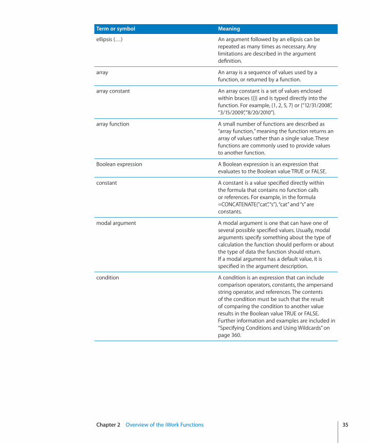
ellipsis (…) An argument followed by an ellipsis can be repeated as many times as necessary. Any limitations are described in the argument definition.
array An array is a sequence of values used by a function, or returned by a function.
array constant An array constant is a set of values enclosed within braces ({}) and is typed directly into the function. For example, {1, 2, 5, 7} or {“12/31/2008”, “3/15/2009”, “8/20/2010”}.
array function A small number of functions are described as “array function,” meaning the function returns an array of values rather than a single value. These functions are commonly used to provide values to another function.
Boolean expression A Boolean expression is an expression that evaluates to the Boolean value TRUE or FALSE.
constant A constant is a value specified directly within the formula that contains no function calls or references. For example, in the formula =CONCATENATE(”cat”, “s”), “cat” and “s” are constants.
modal argument A modal argument is one that can have one of several possible specified values. Usually, modal arguments specify something about the type of calculation the function should perform or about the type of data the function should return. If a modal argument has a default value, it is specified in the argument description.
condition A condition is an expression that can include comparison operators, constants, the ampersand string operator, and references. The contents of the condition must be such that the result of comparing the condition to another value results in the Boolean value TRUE or FALSE. Further information and examples are included in “Specifying Conditions and Using Wildcards” on page 360.

Value TypesA function argument has a type, which specifies what type of information the argument can contain. Functions also return a value of a particular type.
Value Type Description
any If an argument is specified as “any,” it can be a Boolean value, date/time value, duration value, number value, or string value.
Boolean A Boolean value is a logical TRUE (1) or FALSE (0) value or a reference to a cell containing or resulting in a logical TRUE or FALSE value. It is generally the result of evaluating a Boolean expression, but a Boolean value can be specified directly as an argument to a function or as the content of a cell. A common use of a Boolean value is to determine which expression is to be returned by the IF function.
collection An argument that is specified as a collection can be a reference to a single table cell range, an array constant, or an array returned by an array function. An argument specified as collection will have an additional attribute defining the type of values it can contain.
date/time This is a date/time value or a reference to a cell containing a date/time value in any of the formats supported by iWork. If a date/time value is typed into the function, it should be enclosed in quotation marks. You can choose to display only a date or time in a cell, but all date/time values contain both a date and a time.
Although dates can usually be entered directly as strings (for example, “12/31/2010”), using the DATE function insures the date will be interpreted consistently regardless of the date format selected in System Preferences (search for “date format” in the System Preferences window).
36 Chapter 2 Overview of the iWork Functions

Chapter 2 Overview of the iWork Functions 37
Value Type Description
duration A duration is a length of time or a reference to a cell containing a length of time. Duration values consist of weeks (w or weeks), days (d or days), hours (h or hours), minutes (m or minutes), seconds (s or seconds), and milliseconds (ms or milliseconds). A duration value can be entered in one of two formats.
The first format consists of a number, followed by a time period (such as h for hours), optionally followed by a space, and is repeated for other time periods. You can use either the abbreviation for specifying the period, such as “h”, or the full name, such as “hours.” For example, 12h 5d 3m represents a duration of 12 hours, 5 days, and 3 minutes. TIme periods do not have to be entered in order and spaces are not required. 5d 5h is the same as 5h5d. If typed directly into a formula, the string should be enclosed in quotation marks, as in “12h 5d 3m”.
A duration can also be entered as a series of numbers delimited by colons. If this format is used, the seconds argument should be included and end with a decimal followed by the number of milliseconds, which can be 0, if the duration value could be confused with a date/time value. For example, 12:15:30.0 would represent a duration of 12 hours, 15 minutes, and 30 seconds, whereas 12:15:30 would be 12:15:30 a.m. 5:00.0 would represent a duration of exactly 5 minutes. If typed directly into a function, the string should be enclosed in quotation marks, as in “12:15:30.0” or “5:00.0”. If the cell is formatted to a particular duration display, the duration units are applied relative to that duration display and the milliseconds need not be specified.

Value Type Description
list A list is a comma-separated sequence of other values. For example, =CHOOSE(3, “1st”, “second”, 7, “last”). In some cases, the list is enclosed in an additional set of parentheses. For example, =AREAS((B1:B5, C10:C12)).
modal A modal value is a single value, often a number, representing a specific mode for a modal argument. “Modal argument” is defined in “Syntax Elements and Terms Used In Function Definitions” on page 34.
number A number value is a number, a numeric expression, or a reference to a cell containing a numeric expression. If the acceptable values of a number are limited (for example, the number must be greater than 0), this is included within the argument description.
range value A range value is a reference to a single range of cells (can be a single cell). A range value will have an additional attribute defining the type of values it should contain. This will be included within the argument description.
38 Chapter 2 Overview of the iWork Functions

Chapter 2 Overview of the iWork Functions 39
Value Type Description
reference This is a reference to a single cell or a range of cells. If the range is more than one cell, the starting and ending cell are separated by a single colon. For example, =COUNT(A3:D7).
Unless the cell name is unique within all tables, the reference must contain the name of the table if the reference is to a cell on another table. For example, =Table 2::B2. Note that the table name and cell reference are separated by a double colon (::).
If the table is on another sheet, the sheet name must also be included, unless the cell name is unique within all the the sheets. For example, =SUM(Sheet 2::Table 1::C2:G2). The sheet name, table name and cell reference are separated by double colons.
Some functions that accept ranges can operate on ranges that span multiple tables. Assume that you have a file open that has one sheet containing three tables (Table 1, Table 2, Table 3). Assume further that cell C2 in each table contains the number 1. The table-spanning formula =SUM(Table 1:Table 2 :: C2) would sum cell C2 in all tables between Table 1 and Table 2. So the result would be 2. If you drag Table 3 so that it appears between Table 1 and Table 2 in the sidebar, the function will return 3, since it is now summing cell C2 in all three tables (Table 3 is between Table 1 and Table 2).
string A string is zero or more characters, or a reference to a cell containing one or more characters. The characters can consist of any printable characters, including numbers. If a string value is typed into the formula, it must be enclosed in quotation marks. If the string value is somehow limited (for example, the string must represent a date), this is included within the argument description.

Listing of Function CategoriesThere are several categories of functions. For example, some functions perform calculations on date/time values, logical functions give a Boolean (TRUE or FALSE) result, and other functions perform financial calculations. Each of the categories of functions is discussed in a separate chapter.
“Listing of Date and Time Functions” on page 42
“Listing of Duration Functions” on page 64
“Listing of Engineering Functions” on page 72
“Listing of Financial Functions” on page 96
“Listing of Logical and Information Functions” on page 155
“Listing of Numeric Functions” on page 167
“Listing of Reference Functions” on page 206
“Listing of Statistical Functions” on page 225
“Listing of Text Functions” on page 306
“Listing of Trigonometric Functions” on page 326
40 Chapter 2 Overview of the iWork Functions

Chapter 2 Overview of the iWork Functions 41
Pasting from Examples in HelpMany of the examples in help can be copied and pasted directly into a table or, in Numbers, onto a blank canvas. There are two groups of examples which can be copied from help and pasted into a table. The first are individual examples included within help. All such examples begin with an equal sign (=). In the help for the HOUR function, there are two such examples.
To use one of these examples, select the text beginning with the equal sign through the end of the example.
Once this text is highlighted, you can copy it and then paste it into any cell in a table. An alternative to copy and paste is to drag the selection from the example and drop it onto any cell in a table.
The second kind of example that can be copied are example tables included within help. This is the help example table for ACCRINT.
To use an example table, select all the cells in the example table, including the first row.
Once this text is highlighted, you can copy it and then paste it into any cell in a table or onto a blank canvas in a Numbers sheet. Drag and drop cannot be used for this type of example.

42
The date and time functions help you work with dates and times to solve problems such as finding the number of working days between two dates or finding the name of the day of the week a date will fall on.
Listing of Date and Time FunctionsiWork includes these date and time functions for use with tables.
Function Description
“DATE” (page 44) The DATE function combines separate values for year, month, and day and returns a date/time value. Although dates can usually be entered directly as strings (for example, “12/31/2010”), using the DATE function ensures the date will be interpreted consistently regardless of the date format specified in System Preferences (search for “date format” in the System Preferences window).
“DATEDIF” (page 45) The DATEDIF function returns the number of days, months, or years between two dates.
“DATEVALUE” (page 47) The DATEVALUE function converts a date text string and returns a date/time value. This function is provided for compatibility with other spreadsheet programs.
“DAY” (page 47) The DAY function returns the day of the month for a given date/time value.
“DAYNAME” (page 48) The DAYNAME function returns the name of the day of the week from a date/time value or a number. Day 1 is Sunday.
“DAYS360” (page 49) The DAYS360 function returns the number of days between two dates based on twelve 30-day months and a 360-day year.
3Date and Time Functions

Chapter 3 Date and Time Functions 43
Function Description
“EDATE” (page 50) The EDATE function returns a date that is some number of months before or after a given date.
“EOMONTH” (page 51) The EOMONTH function returns a date that is the last day of the month some number of months before or after a given date.
“HOUR” (page 51) The HOUR function returns the hour for a given date/time value.
“MINUTE” (page 52) The MINUTE function returns the minutes for a given date/time value.
“MONTH” (page 53) The MONTH function returns the month for a given date/time value.
“MONTHNAME” (page 54) The MONTHNAME function returns the name of the month from a number. Month 1 is January.
“NETWORKDAYS” (page 54) The NETWORKDAYS function returns the number of working days between two dates. Working days exclude weekends and any other specified dates.
“NOW” (page 55) The NOW function returns the current date/time value from the system clock.
“SECOND” (page 56) The SECOND function returns the seconds for a given date/time value.
“TIME” (page 56) The TIME function converts separate values for hours, minutes, and seconds into a date/time value.
“TIMEVALUE” (page 57) The TIMEVALUE function returns the time as a decimal fraction of a 24-hour day from a given date/time value or from a text string.
“TODAY” (page 58) The TODAY function returns the current system date. The time is set to 12:00 a.m.

Function Description
“WEEKDAY” (page 59) The WEEKDAY function returns a number that is the day of the week for a given date.
“WEEKNUM” (page 60) The WEEKNUM function returns the number of the week within the year for a given date.
“WORKDAY” (page 61) The WORKDAY function returns the date that is the given number of working days before or after a given date. Working days exclude weekends and any other dates specifically excluded.
“YEAR” (page 62) The YEAR function returns the year for a given date/time value.
“YEARFRAC” (page 63) The YEARFRAC function finds the fraction of a year represented by the number of whole days between two dates.
DATEThe DATE function combines separate values for year, month, and day and returns a date/time value. Although dates can usually be entered directly as strings (for example, “12/31/2010”), using the DATE function ensures the date will be interpreted consistently regardless of the date format specified in System Preferences (search for “date format” in the System Preferences window).
DATE(year, month, day)
 year:� The year to include in the value returned. year is a number value. The value isn’t converted. If you specify 10, the year 10 is used, not the year 1910 or 2010.
 month:� The month to include in the value returned. month is a number and should be in the range 1 to 12.
 day:� The day to include in the value returned. day is a number value and should be in the range 1 to the number of days in month.
Examples
If A1 contains 2014, A2 contains 11, and A3 contains 10:
=DATE(A1, A2, A3) returns Nov 10, 2014, which is displayed according to the cell’s current format.
=DATE(A1, A3, A2) returns Oct 11, 2014.
=DATE(2012, 2, 14) returns Feb 14, 2012.
Related TopicsFor related functions and additional information, see:
“DURATION” on page 70
44 Chapter 3 Date and Time Functions

Chapter 3 Date and Time Functions 45
“TIME” on page 56
“Listing of Date and Time Functions” on page 42
“Value Types” on page 36
“The Elements of Formulas” on page 15
“Using the Keyboard and Mouse to Create and Edit Formulas” on page 26
“Pasting from Examples in Help” on page 41
DATEDIFThe DATEDIF function returns the number of days, months, or years between two dates.
DATEDIF(start-date, end-date, calc-method)
 start-date:� The starting date. start-date is a date/time value.
 end-date:� The ending date. end-date is a date/time value.
 calc-method:� Specifies how to express the time difference and how dates in different years or months are handled.
“D”:� Count the number of days between the start and end dates.
“M”:� Count the number of months between the start and end dates.
“Y”:� Count the number of years between the start and end dates.
“MD”:� Count the days between the start and end dates, ignoring months and years. The month in end-date is considered to be the month in start-date. If the starting day is after the ending day, the count starts from the ending day as if it were in the preceding month. The year of the end-date is used to check for a leap year.
“YM”:� Count the number of whole months between the start and end dates, ignoring the year. If the starting month/day is before the ending month/day, the dates are treated as though they are in the same year. If the starting month/day is after the ending month/day, the dates are treated as though they are in consecutive years.
“YD”:� Count the number of days between the start and end dates, ignoring the year. If the starting month/day is before the ending month/day, the dates are treated as though they are in the same year. If the starting month/day is after the ending month/day, the dates are treated as though they are in consecutive years.

Examples
If A1 contains the date/time value 4/6/88 and A2 contains the date/time value 10/30/06:
=DATEDIF(A1, A2, “D”) returns 6781, the number of days between April 6, 1988, and October 30, 2006.
=DATEDIF(A1, A2, “M”) returns 222, the number of whole months between April 6, 1988, and October 30, 2006.
=DATEDIF(A1, A2, “Y”) returns 18, the number of whole years between April 6, 1988, and October 30, 2006.
=DATEDIF(A1, A2, “MD”) returns 24, the number of days between the sixth day of a month and the thirtieth day of the same month.
=DATEDIF(A1, A2, “YM”) returns 6, the number of months between April and the following October in any year.
=DATEDIF(A1, A2, “YD”) returns 207, the number of days between April 6 and the following October 30 in any year.
=DATEDIF(”04/06/1988”, NOW(), “Y”) & “ years, “ & DATEDIF(”04/06/1988”, NOW(), “YM”) & “ months, and “ & DATEDIF(”04/06/1988”, NOW(), “MD”) & “ days” returns the current age of someone born on April 6, 1988.
Related TopicsFor related functions and additional information, see:
“DAYS360” on page 49
“NETWORKDAYS” on page 54
“NOW” on page 55
“YEARFRAC” on page 63
“Listing of Date and Time Functions” on page 42
“Value Types” on page 36
“The Elements of Formulas” on page 15
“Using the Keyboard and Mouse to Create and Edit Formulas” on page 26
“Pasting from Examples in Help” on page 41
46 Chapter 3 Date and Time Functions
Chapter 3 Date and Time Functions 47
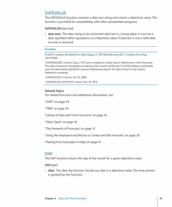
DATEVALUEThe DATEVALUE function converts a date text string and returns a date/time value. This function is provided for compatibility with other spreadsheet programs.
DATEVALUE(date-text)
 date-text:� The date string to be converted. date-text is a string value. It must be a date specified within quotations or a date/time value. If date-text is not a valid date, an error is returned.
Examples
If cell B1 contains the date/time value August 2, 1979 06:30:00 and cell C1 contains the string 10/16/2008:
=DATEVALUE(B1) returns Aug 2, 1979, and is treated as a date value if referenced in other formulas. The value returned is formatted according to the current cell format. A cell formatted as Automatic uses the date format specified in System Preferences (search for “date format” in the System Preferences window).
=DATEVALUE(C1) returns Oct 16, 2008.
=DATEVALUE(“12/29/1974”) returns Dec 29, 1979.
Related TopicsFor related functions and additional information, see:
“DATE” on page 44
“TIME” on page 56
“Listing of Date and Time Functions” on page 42
“Value Types” on page 36
“The Elements of Formulas” on page 15
“Using the Keyboard and Mouse to Create and Edit Formulas” on page 26
“Pasting from Examples in Help” on page 41
DAYThe DAY function returns the day of the month for a given date/time value.
DAY(date)
 date:� The date the function should use. date is a date/time value. The time portion is ignored by this function.

Examples
=DAY(”4/6/88 11:59:22 PM”) returns 6.
=DAY(“5/12/2009”) returns 12.
Related TopicsFor related functions and additional information, see:
“DAYNAME” on page 48
“HOUR” on page 51
“MINUTE” on page 52
“MONTH” on page 53
“SECOND” on page 56
“YEAR” on page 62
“Listing of Date and Time Functions” on page 42
“Value Types” on page 36
“The Elements of Formulas” on page 15
“Using the Keyboard and Mouse to Create and Edit Formulas” on page 26
“Pasting from Examples in Help” on page 41
DAYNAMEThe DAYNAME function returns the name of the day of the week from a date/time value or a number. Day 1 is Sunday.
DAYNAME(day-num)
 day-num:� The desired day of the week. day-num is a date/time value, or number value in the range 1 to 7. If day-num has a decimal portion, it is ignored.
Examples
If B1 contains the date/time value August 2, 1979 06:30:00, C1 contains the string 10/16/2008, and D1 contains 6:
=DAYNAME(B1) returns Thursday.
=DAYNAME(C1) returns Thursday.
=DAYNAME(D1) returns Friday.
=DAYNAME(“12/29/1974”) returns Sunday.
48 Chapter 3 Date and Time Functions

Chapter 3 Date and Time Functions 49
Related TopicsFor related functions and additional information, see:
“DAY” on page 47
“MONTHNAME” on page 54
“WEEKDAY” on page 59
“Listing of Date and Time Functions” on page 42
“Value Types” on page 36
“The Elements of Formulas” on page 15
“Using the Keyboard and Mouse to Create and Edit Formulas” on page 26
“Pasting from Examples in Help” on page 41
DAYS360The DAYS360 function returns the number of days between two dates based on twelve 30-day months and a 360-day year.
DAYS360(start-date, end-date, use-euro-method)
 start-date:� The starting date. start-date is a date/time value.
 end-date:� The ending date. end-date is a date/time value.
 use-euro-method:� An optional value that specifies whether to use the NASD or European method for dates falling on the 31st of a month.
NASD method (0, FALSE, or omitted):� Use the NASD method for dates falling on the 31st of a month.
EURO method (1 or TRUE):� Use the European method for dates falling on the 31st of a month.
Examples
=DAYS360(”12/20/2008”, “3/31/2009”) returns 101d.
=DAYS360(”2/27/2008”, “3/31/2009”,0) returns 394d.
=DAYS360(”2/27/2008”, “3/31/2009”,1) returns 393d, as the European calculation method is used.
Related TopicsFor related functions and additional information, see:
“DATEDIF” on page 45
“NETWORKDAYS” on page 54

“YEARFRAC” on page 63
“Listing of Date and Time Functions” on page 42
“Value Types” on page 36
“The Elements of Formulas” on page 15
“Using the Keyboard and Mouse to Create and Edit Formulas” on page 26
“Pasting from Examples in Help” on page 41
EDATEThe EDATE function returns a date that is some number of months before or after a given date.
EDATE(start-date, month-offset)
 start-date:� The starting date. start-date is a date/time value.
 month-offset: The number of months before or after the starting date. month-offset is a number value. A negative month-offset is used to specify a number of months before the starting date and a positive month-offset is used to specify a number of months after the starting date.
Examples
=EDATE(”1/15/2000”, 1) returns 2/15/2000, the date one month later.
=EDATE(”1/15/2000”, -24) returns 1/15/1998, the date 24 months earlier.
Related TopicsFor related functions and additional information, see:
“EOMONTH” on page 51
“Listing of Date and Time Functions” on page 42
“Value Types” on page 36
“The Elements of Formulas” on page 15
“Using the Keyboard and Mouse to Create and Edit Formulas” on page 26
“Pasting from Examples in Help” on page 41
50 Chapter 3 Date and Time Functions

Chapter 3 Date and Time Functions 51
EOMONTHThe EOMONTH function returns a date that is the last day of the month some number of months before or after a given date.
EOMONTH(start-date, month-offset)
 start-date:� The starting date. start-date is a date/time value.
 month-offset: The number of months before or after the starting date. month-offset is a number value. A negative month-offset is used to specify a number of months before the starting date and a positive month-offset is used to specify a number of months after the starting date.
Examples
=EOMONTH(”5/15/2010”, 5) returns Oct 31, 2010, the last day of the month five months after May 2010.
=EOMONTH(”5/15/2010”, -5) returns Dec 31, 2009, the last day of the month five months before May 2010.
Related TopicsFor related functions and additional information, see:
“EDATE” on page 50
“Listing of Date and Time Functions” on page 42
“Value Types” on page 36
“The Elements of Formulas” on page 15
“Using the Keyboard and Mouse to Create and Edit Formulas” on page 26
“Pasting from Examples in Help” on page 41
HOURThe HOUR function returns the hour for a given date/time value.
HOUR(time)
 time:� The time the function should use. time is a date/time value. The date portion is ignored by this function.
Usage NotesThe hour returned is in 24-hour format (0 is midnight, 23 is 11:00 p.m.). Â
Examples
=HOUR(NOW()) returns the current hour of the day.
=HOUR(”4/6/88 11:59:22 AM”) returns 11.

Related TopicsFor related functions and additional information, see:
“DAY” on page 47
“MINUTE” on page 52
“MONTH” on page 53
“SECOND” on page 56
“YEAR” on page 62
“Listing of Date and Time Functions” on page 42
“Value Types” on page 36
“The Elements of Formulas” on page 15
“Using the Keyboard and Mouse to Create and Edit Formulas” on page 26
“Pasting from Examples in Help” on page 41
MINUTEThe MINUTE function returns the minutes for a given date/time value.
MINUTE(time)
 time:� The time the function should use. time is a date/time value. The date portion is ignored by this function.
Example
=MINUTE(”4/6/88 11:59:22 AM”) returns 59.
Related TopicsFor related functions and additional information, see:
“DAY” on page 47
“HOUR” on page 51
“MONTH” on page 53
“SECOND” on page 56
“YEAR” on page 62
“Listing of Date and Time Functions” on page 42
52 Chapter 3 Date and Time Functions

Chapter 3 Date and Time Functions 53
“Value Types” on page 36
“The Elements of Formulas” on page 15
“Using the Keyboard and Mouse to Create and Edit Formulas” on page 26
“Pasting from Examples in Help” on page 41
MONTHThe MONTH function returns the month for a given date/time value.
MONTH(date)
 date:� The date the function should use. date is a date/time value. The time portion is ignored by this function.
Example
=MONTH(”April 6, 1988 11:59:22 AM”) returns 4.
Related TopicsFor related functions and additional information, see:
“DAY” on page 47
“HOUR” on page 51
“MINUTE” on page 52
“MONTHNAME” on page 54
“SECOND” on page 56
“YEAR” on page 62
“Listing of Date and Time Functions” on page 42
“Value Types” on page 36
“The Elements of Formulas” on page 15
“Using the Keyboard and Mouse to Create and Edit Formulas” on page 26
“Pasting from Examples in Help” on page 41
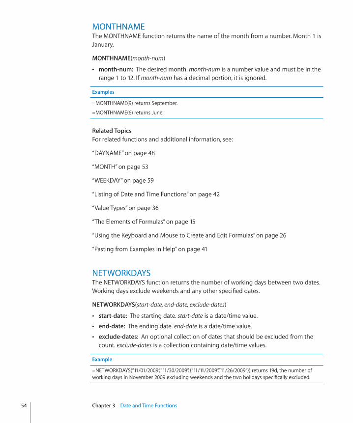
MONTHNAMEThe MONTHNAME function returns the name of the month from a number. Month 1 is January.
MONTHNAME(month-num)
 month-num:� The desired month. month-num is a number value and must be in the range 1 to 12. If month-num has a decimal portion, it is ignored.
Examples
=MONTHNAME(9) returns September.
=MONTHNAME(6) returns June.
Related TopicsFor related functions and additional information, see:
“DAYNAME” on page 48
“MONTH” on page 53
“WEEKDAY” on page 59
“Listing of Date and Time Functions” on page 42
“Value Types” on page 36
“The Elements of Formulas” on page 15
“Using the Keyboard and Mouse to Create and Edit Formulas” on page 26
“Pasting from Examples in Help” on page 41
NETWORKDAYSThe NETWORKDAYS function returns the number of working days between two dates. Working days exclude weekends and any other specified dates.
NETWORKDAYS(start-date, end-date, exclude-dates)
 start-date:� The starting date. start-date is a date/time value.
 end-date:� The ending date. end-date is a date/time value.
 exclude-dates:� An optional collection of dates that should be excluded from the count. exclude-dates is a collection containing date/time values.
Example
=NETWORKDAYS(”11/01/2009”, “11/30/2009”, {”11/11/2009”,”11/26/2009”}) returns 19d, the number of working days in November 2009 excluding weekends and the two holidays specifically excluded.
54 Chapter 3 Date and Time Functions

Chapter 3 Date and Time Functions 55
Related TopicsFor related functions and additional information, see:
“DATEDIF” on page 45
“DAYS360” on page 49
“WORKDAY” on page 61
“YEARFRAC” on page 63
“Listing of Date and Time Functions” on page 42
“Value Types” on page 36
“The Elements of Formulas” on page 15
“Using the Keyboard and Mouse to Create and Edit Formulas” on page 26
“Pasting from Examples in Help” on page 41
NOWThe NOW function returns the current date/time value from the system clock.
NOW()
Usage NotesThe NOW function does not have any arguments. However, you must include the Âparentheses: =NOW().
Example
=NOW() returns October 4, 2008 10:47 am, if your file is updated on October 4, 2008, at 10:47 a.m.
Related TopicsFor related functions and additional information, see:
“TODAY” on page 58
“Listing of Date and Time Functions” on page 42
“Value Types” on page 36
“The Elements of Formulas” on page 15
“Using the Keyboard and Mouse to Create and Edit Formulas” on page 26
“Pasting from Examples in Help” on page 41

SECONDThe SECOND function returns the seconds for a given date/time value.
SECOND(time)
 time:� The time the function should use. time is a date/time value. The date portion is ignored by this function.
Example
=SECOND(”4/6/88 11:59:22 am”) returns 22.
Related TopicsFor related functions and additional information, see:
“DAY” on page 47
“HOUR” on page 51
“MINUTE” on page 52
“Listing of Date and Time Functions” on page 42
“Value Types” on page 36
“The Elements of Formulas” on page 15
“Using the Keyboard and Mouse to Create and Edit Formulas” on page 26
“Pasting from Examples in Help” on page 41
TIMEThe TIME function converts separate values for hours, minutes, and seconds into a date/time value.
TIME(hours, minutes, seconds)
 hours:� The number of hours to include in the value returned. hours is a number value. If hours has a decimal portion, it is ignored.
 minutes:� The number of minutes to include in the value returned. minutes is a number value. If minutes has a decimal portion, it is ignored.
 seconds:� The number of seconds to include in the value returned. seconds is a number value. If seconds has a decimal portion, it is ignored.
Usage NotesYou can specify hour, minute, and second values greater than 24, 60, and 60, Ârespectively. If the hours, minutes, and seconds add up to more than 24 hours, 24 hours are repeatedly subtracted until the value is less than 24 hours.
56 Chapter 3 Date and Time Functions

Chapter 3 Date and Time Functions 57
Examples
=TIME(12, 0, 0) returns 12:00 pm.
=TIME(16, 45, 30) returns 4:45 pm.
=TIME(0, 900, 0) returns 3:00 pm.
=TIME(60, 0, 0) returns 12:00 pm.
=TIME(4.25, 0, 0) returns 4:00 am.
Related TopicsFor related functions and additional information, see:
“DATE” on page 44
“DATEVALUE” on page 47
“DURATION” on page 70
“Listing of Date and Time Functions” on page 42
“Value Types” on page 36
“The Elements of Formulas” on page 15
“Using the Keyboard and Mouse to Create and Edit Formulas” on page 26
“Pasting from Examples in Help” on page 41
TIMEVALUEThe TIMEVALUE function returns the time as a decimal fraction of a 24-hour day from a given date/time value or from a text string.
TIMEVALUE(time)
 time:� The time the function should use. time is a date/time value. The date portion is ignored by this function.
Examples
=TIMEVALUE(”4/6/88 12:00”) returns 0.5 (noon represents one-half of the day).
=TIMEVALUE(”12:00:59”) returns 0.5007 (rounded to four decimal places of accuracy).
=TIMEVALUE(”9:00 pm”) returns 0.875 (21 hours, or 9:00 p.m., divided by 24).
Related TopicsFor related functions and additional information, see:
“Listing of Date and Time Functions” on page 42

“Value Types” on page 36
“The Elements of Formulas” on page 15
“Using the Keyboard and Mouse to Create and Edit Formulas” on page 26
“Pasting from Examples in Help” on page 41
TODAYThe TODAY function returns the current system date. The time is set to 12:00 a.m.
TODAY()
Usage NotesThe TODAY function does not have any arguments. However, you must include the Âparentheses: =TODAY().
The displayed date is updated every time you open or modify your file. Â
You can use the NOW function to get the current date and time and to format the Âcell to display both.
Example
=TODAY() returns Apr 6, 2008, when calculated on April 6, 2008.
Related TopicsFor related functions and additional information, see:
“NOW” on page 55
“Listing of Date and Time Functions” on page 42
“Value Types” on page 36
“The Elements of Formulas” on page 15
“Using the Keyboard and Mouse to Create and Edit Formulas” on page 26
“Pasting from Examples in Help” on page 41
58 Chapter 3 Date and Time Functions

Chapter 3 Date and Time Functions 59
WEEKDAYThe WEEKDAY function returns a number that is the day of the week for a given date.
WEEKDAY(date, first-day)
 date:� The date the function should use. date is a date/time value. The time portion is ignored by this function.
 first-day: An optional value that specifies how days are numbered.
Sunday is 1 (1 or omitted):� Sunday is the first day (day 1) of the week and Saturday is day 7.
Monday is 1 (2):� Monday is the first day (day 1) of the week and Sunday is day 7.
Monday is 0 (3):� Monday is the first day (day 0) of the week and Sunday is day 6.
Examples
=WEEKDAY(”Apr 6, 1988”, 1) returns 4 (Wednesday, the fourth day if you start counting Sunday as day 1).
=WEEKDAY(”Apr 6, 1988”) returns the same value as the preceding example (numbering scheme 1 is used if no number-scheme argument is specified).
=WEEKDAY(”Apr 6, 1988”, 2) returns 3 (Wednesday, the third day if you start counting Monday as day 1).
=WEEKDAY(”Apr 6, 1988”, 3) returns 2 (Wednesday, day number 2 if you start counting Monday as day 0).
Related TopicsFor related functions and additional information, see:
“DAYNAME” on page 48
“MONTHNAME” on page 54
“Listing of Date and Time Functions” on page 42
“Value Types” on page 36
“The Elements of Formulas” on page 15
“Using the Keyboard and Mouse to Create and Edit Formulas” on page 26
“Pasting from Examples in Help” on page 41

WEEKNUMThe WEEKNUM function returns the number of the week within the year for a given date.
WEEKNUM(date, first-day)
 date:� The date the function should use. date is a date/time value. The time portion is ignored by this function.
 first-day: An optional value that specifies whether weeks should begin on Sunday or Monday.
Sunday is 1 (1 or omitted):� Sunday is the first day (day 1) of the week and Saturday is day 7.
Monday is 1 (2):� Monday is the first day (day 1) of the week and Sunday is day 7.
Example
=WEEKNUM(”7/12/2009”,1) returns 29.
=WEEKNUM(”7/12/2009”,2) returns 28.
Related TopicsFor related functions and additional information, see:
“DAY” on page 47
“HOUR” on page 51
“MINUTE” on page 52
“MONTH” on page 53
“SECOND” on page 56
“YEAR” on page 62
“Listing of Date and Time Functions” on page 42
“Value Types” on page 36
“The Elements of Formulas” on page 15
“Using the Keyboard and Mouse to Create and Edit Formulas” on page 26
“Pasting from Examples in Help” on page 41
60 Chapter 3 Date and Time Functions

Chapter 3 Date and Time Functions 61
WORKDAYThe WORKDAY function returns the date that is the given number of working days before or after a given date. Working days exclude weekends and any other dates specifically excluded.
WORKDAY(date, work-days, exclude-dates)
 date:� The date the function should use. date is a date/time value. The time portion is ignored by this function.
 work-days:� The number of working days before or after the given date. work-days is a number value. It is positive if the desired date is after date and negative if the desired date is before date.
 exclude-dates:� An optional collection of dates that should be excluded from the count. exclude-dates is a collection containing date/time values.
Example
=WORKDAY(”11/01/2009”, 20, {”11/11/2009”,”11/26/2009”}) returns Dec 1, 2009, the work day 20 days after 11/01/2009 excluding weekends and the two holidays specifically excluded.
Related TopicsFor related functions and additional information, see:
“NETWORKDAYS” on page 54
“Listing of Date and Time Functions” on page 42
“Value Types” on page 36
“The Elements of Formulas” on page 15
“Using the Keyboard and Mouse to Create and Edit Formulas” on page 26
“Pasting from Examples in Help” on page 41

YEARThe YEAR function returns the year for a given date/time value.
YEAR(date)
 date:� The date the function should use. date is a date/time value. The time portion is ignored by this function.
Examples
=YEAR(”April 6, 2008”) returns 2008.
=YEAR(NOW()) returns 2009 when evaluated on June 4, 2009.
Related TopicsFor related functions and additional information, see:
“DAY” on page 47
“HOUR” on page 51
“MINUTE” on page 52
“MONTH” on page 53
“SECOND” on page 56
“Listing of Date and Time Functions” on page 42
“Value Types” on page 36
“The Elements of Formulas” on page 15
“Using the Keyboard and Mouse to Create and Edit Formulas” on page 26
“Pasting from Examples in Help” on page 41
62 Chapter 3 Date and Time Functions

Chapter 3 Date and Time Functions 63
YEARFRACThe YEARFRAC function finds the fraction of a year represented by the number of whole days between two dates.
YEARFRAC(start-date, end-date, days-basis)
 start-date:� The starting date. start-date is a date/time value.
 end-date:� The ending date. end-date is a date/time value.
 days-basis:� An optional argument specifying the number of days per month and days per year used in the calculations.
30/360 (0 or omitted):� 30 days in a month, 360 days in a year, using the NASD method for dates falling on the 31st of a month.
actual/actual (1):� Actual days in each month, actual days in each year.
actual/360 (2):� Actual days in each month, 360 days in a year.
actual/365 (3):� Actual days in each month, 365 days in a year.
30E/360 (4):� 30 days in a month, 360 days in a year, using the European method for dates falling on the 31st of a month (European 30/360).
Examples
=YEARFRAC(”12/15/2009”, “6/30/2010”,0) returns 0.541666667.
=YEARFRAC(”12/15/2009”, “6/30/2010”,1) returns 0.539726027.
=YEARFRAC(”12/15/2009”, “6/30/2010”,2) returns 0.547222222.
=YEARFRAC(”12/15/2009”, “6/30/2010”,3) returns 0.539726027.
=YEARFRAC(”12/15/2009”, “6/30/2010”,4) returns 0.541666667.
Related TopicsFor related functions and additional information, see:
“DATEDIF” on page 45
“DAYS360” on page 49
“NETWORKDAYS” on page 54
“Listing of Date and Time Functions” on page 42
“Value Types” on page 36
“The Elements of Formulas” on page 15
“Using the Keyboard and Mouse to Create and Edit Formulas” on page 26
“Pasting from Examples in Help” on page 41

64
The duration functions help you work with periods of time (durations) by converting between different time periods, such as hours, days, and weeks.
Listing of Duration FunctionsiWork provides these duration functions for use with tables.
Function Description
“DUR2DAYS” (page 65) The DUR2DAYS function converts a duration value to a number of days.
“DUR2HOURS” (page 65) The DUR2HOURS function converts a duration value to a number of hours.
“DUR2MILLISECONDS” (page 66) The DUR2MILLISECONDS function converts a duration value to a number of milliseconds.
“DUR2MINUTES” (page 67) The DUR2MINUTES function converts a duration value to a number of minutes.
“DUR2SECONDS” (page 68) The DUR2SECONDS function converts a duration value to a number of seconds.
“DUR2WEEKS” (page 69) The DUR2WEEKS function converts a duration value to a number of weeks.
“DURATION” (page 70) The DURATION function combines separate values for weeks, days, hours, minutes, seconds, and milliseconds and returns a duration value.
“STRIPDURATION” (page 71) The STRIPDURATION function evaluates a given value and returns either the number of days represented, if a duration value, or the given value. This function is included for compatibility with other spreadsheet applications.
4Duration Functions

Chapter 4 Duration Functions 65
DUR2DAYSThe DUR2DAYS function converts a duration value to a number of days.
DUR2DAYS(duration)
 duration:� The length of time to be converted. duration is a duration value.
Examples
=DUR2DAYS(”2w 3d 2h 10m 0s 5ms”) returns 17.09027784.
=DUR2DAYS(”10:0:13:00:05.500”) returns 70.5417302.
Related TopicsFor related functions and additional information, see:
“DUR2HOURS” on page 65
“DUR2MILLISECONDS” on page 66
“DUR2MINUTES” on page 67
“DUR2SECONDS” on page 68
“DUR2WEEKS” on page 69
“Listing of Duration Functions” on page 64
“Value Types” on page 36
“The Elements of Formulas” on page 15
“Using the Keyboard and Mouse to Create and Edit Formulas” on page 26
“Pasting from Examples in Help” on page 41
DUR2HOURSThe DUR2HOURS function converts a duration value to a number of hours.
DUR2HOURS(duration)
 duration:� The length of time to be converted. duration is a duration value.
Examples
=DUR2HOURS(”2w 3d 2h 10m 0s 5ms”) returns 410.1666681.
=DUR2HOURS(”10:0:13:00:05.500”) returns 1693.001528.

Related TopicsFor related functions and additional information, see:
“DUR2DAYS” on page 65
“DUR2MILLISECONDS” on page 66
“DUR2MINUTES” on page 67
“DUR2SECONDS” on page 68
“DUR2WEEKS” on page 69
“Listing of Duration Functions” on page 64
“Value Types” on page 36
“The Elements of Formulas” on page 15
“Using the Keyboard and Mouse to Create and Edit Formulas” on page 26
“Pasting from Examples in Help” on page 41
DUR2MILLISECONDSThe DUR2MILLISECONDS function converts a duration value to a number of milliseconds.
DUR2MILLISECONDS(duration)
 duration:� The length of time to be converted. duration is a duration value.
Examples
=DUR2MILLISECONDS(”2w 3d 2h 10m 0s 5ms”) returns 1476600005.
=DUR2MILLISECONDS(”10:0:13:00:05.500”) returns 6094805500.
Related TopicsFor related functions and additional information, see:
“DUR2DAYS” on page 65
“DUR2HOURS” on page 65
“DUR2MINUTES” on page 67
“DUR2SECONDS” on page 68
“DUR2WEEKS” on page 69
“Listing of Duration Functions” on page 64
66 Chapter 4 Duration Functions

Chapter 4 Duration Functions 67
“Value Types” on page 36
“The Elements of Formulas” on page 15
“Using the Keyboard and Mouse to Create and Edit Formulas” on page 26
“Pasting from Examples in Help” on page 41
DUR2MINUTESThe DUR2MINUTES function converts a duration value to a number of minutes.
DUR2MINUTES(duration)
 duration:� The length of time to be converted. duration is a duration value.
Examples
=DUR2MINUTES(”2w 3d 2h 10m 0s 5ms”) returns 24610.0000833333.
=DUR2MINUTES(”10:0:13:00:05.500”) returns 101580.091666667.
Related TopicsFor related functions and additional information, see:
“DUR2DAYS” on page 65
“DUR2HOURS” on page 65
“DUR2MILLISECONDS” on page 66
“DUR2SECONDS” on page 68
“DUR2WEEKS” on page 69
“Listing of Duration Functions” on page 64
“Value Types” on page 36
“The Elements of Formulas” on page 15
“Using the Keyboard and Mouse to Create and Edit Formulas” on page 26
“Pasting from Examples in Help” on page 41

DUR2SECONDSThe DUR2SECONDS function converts a duration value to a number of seconds.
DUR2SECONDS(duration)
 duration:� The length of time to be converted. duration is a duration value.
Examples
=DUR2SECONDS(”2w 3d 2h 10m 0s 5ms”) returns 1476600.005.
=DUR2SECONDS(”10:0:13:00:05.500”) returns 6094805.5.
Related TopicsFor related functions and additional information, see:
“DUR2DAYS” on page 65
“DUR2HOURS” on page 65
“DUR2MILLISECONDS” on page 66
“DUR2MINUTES” on page 67
“DUR2WEEKS” on page 69
“Listing of Duration Functions” on page 64
“Value Types” on page 36
“The Elements of Formulas” on page 15
“Using the Keyboard and Mouse to Create and Edit Formulas” on page 26
“Pasting from Examples in Help” on page 41
68 Chapter 4 Duration Functions

Chapter 4 Duration Functions 69
DUR2WEEKSThe DUR2WEEKS function converts a duration value to a number of weeks.
DUR2WEEKS(duration)
 duration:� The length of time to be converted. duration is a duration value.
Examples
=DUR2WEEKS(”2w 3d 2h 10m 0s 5ms”) returns 2.44146826223545.
=DUR2WEEKS(”10:0:13:00:05.500”) returns 10.0773900462963.
Related TopicsFor related functions and additional information, see:
“DUR2DAYS” on page 65
“DUR2HOURS” on page 65
“DUR2MILLISECONDS” on page 66
“DUR2MINUTES” on page 67
“DUR2SECONDS” on page 68
“Listing of Duration Functions” on page 64
“Value Types” on page 36
“The Elements of Formulas” on page 15
“Using the Keyboard and Mouse to Create and Edit Formulas” on page 26
“Pasting from Examples in Help” on page 41

DURATIONThe DURATION function combines separate values for weeks, days, hours, minutes, seconds, and milliseconds and returns a duration value.
DURATION(weeks, days, hours, minutes, seconds, milliseconds)
 weeks:� A value representing the number of weeks. weeks is a number value.
 days:� An optional value representing the number of days. days is a number value.
 hours:� An optional value representing the number of hours. hours is a number value.
 minutes:� An optional value representing the number of minutes. minutes is a number value.
 seconds:� An optional value representing the number of seconds. seconds is a number value.
 milliseconds:� An optional value representing the number of milliseconds. milliseconds is a number value.
Usage Notes An argument that is 0 can be omitted, but the comma must be included if later Âvalues are included. For example, =DURATION(, ,12, 3) would return a duration value of 12h 3m (12 hours and 3 minutes).
Negative values are permitted. For example, =DURATION(0, 2, -24) would return a Âduration of 1 day (2 days minus 24 hours).
Examples
=DURATION(1) returns 1w (1 week).
=DURATION(,,1) returns 1h (1 hour).
=DURATION(1.5) returns 1w 3d 12h (1 week, 3 days, 12 hours or 1.5 weeks).
=DURATION(3, 2, 7, 10, 15.3505) returns 3w 2d 7h 10m 15s 350ms (3 weeks, 2 days, 7 hours, 10 minutes, 15 seconds, 350 milliseconds).
Related TopicsFor related functions and additional information, see:
“DATE” on page 44
“TIME” on page 56
“Listing of Duration Functions” on page 64
“Value Types” on page 36
“The Elements of Formulas” on page 15
“Using the Keyboard and Mouse to Create and Edit Formulas” on page 26
“Pasting from Examples in Help” on page 41
70 Chapter 4 Duration Functions

Chapter 4 Duration Functions 71
STRIPDURATIONThe STRIPDURATION function evaluates a given value and returns either the number of days represented, if a duration value, or the given value. This function is included for compatibility with other spreadsheet applications.
STRIPDURATION(any-value)
 any-value:� A value. any-value can contain any value type.
Usage NotesIf  any-value is a duration value, the result is the same as for DUR2DAYS; otherwise any-value is returned.
This function may be automatically inserted when a Numbers ’08 document is Âupgraded, or an Excel or Appleworks document is imported. It is removed in any copy of the file saved as a Numbers ’08 or Excel document.
Examples
=STRIPDURATION(”1w”) returns 7, the equivalent of one week in days.
=STRIPDURATION(12) returns 12; since it was not a duration value it is returned.
=STRIPDURATION (”abc”) returns “abc”.
Related TopicsFor related functions and additional information, see:
“Listing of Duration Functions” on page 64
“Value Types” on page 36
“The Elements of Formulas” on page 15
“Using the Keyboard and Mouse to Create and Edit Formulas” on page 26
“Pasting from Examples in Help” on page 41

72
The engineering functions help you calculate some common engineering values and convert between different numeric bases.
Listing of Engineering FunctionsiWork provides these engineering functions for use with tables.
Function Description
“BASETONUM” (page 73) The BASETONUM function converts a number of the specified base into a number in base 10.
“BESSELJ” (page 74) The BESSELJ function returns the integer Bessel function J
n(x).
“BESSELY” (page 75) The BESSELY function returns the integer Bessel function Y
n(x).
“BIN2DEC” (page 76) The BIN2DEC function converts a binary number to the corresponding decimal number.
“BIN2HEX” (page 77) The BIN2HEX function converts a binary number to the corresponding hexadecimal number.
“BIN2OCT” (page 78) The BIN2OCT function converts a binary number to the corresponding octal number.
“CONVERT” (page 79) The CONVERT function converts a number from one measurement system to its corresponding value in another measurement system.
“DEC2BIN” (page 83) The DEC2BIN function converts a decimal number to the corresponding binary number.
“DEC2HEX” (page 84) The DEC2HEX function converts a decimal number to the corresponding hexadecimal number.
5Engineering Functions

Chapter 5 Engineering Functions 73
Function Description
“DEC2OCT” (page 85) The DEC2OCT function converts a decimal number to the corresponding octal number.
“DELTA” (page 86) The DELTA function determines whether two values are exactly equal.
“ERF” (page 87) The ERF function returns the error function integrated between two values.
“ERFC” (page 87) The ERFC function returns the complementary ERF function integrated between a given lower bound and infinity.
“GESTEP” (page 88) The GESTEP function determines if one value is greater than or exactly equal to another value.
“HEX2BIN” (page 89) The HEX2BIN function converts a hexadecimal number to the corresponding binary number.
“HEX2DEC” (page 90) The HEX2DEC function converts a hexadecimal number to the corresponding decimal number.
“HEX2OCT” (page 91) The HEX2OCT function converts a hexadecimal number to the corresponding octal number.
“NUMTOBASE” (page 92) The NUMTOBASE function converts a number from base 10 into a number in the specified base.
“OCT2BIN” (page 93) The OCT2BIN function converts an octal number to the corresponding binary number.
“OCT2DEC” (page 94) The OCT2DEC function converts an octal number to the corresponding decimal number.
“OCT2HEX” (page 95) The OCT2HEX function converts an octal number to the corresponding hexadecimal number.
BASETONUMThe BASETONUM function converts a number of the specified base into a number in base 10.
BASETONUM(convert-string, base)
 convert-string:� The string representing the number to be converted. convert-string is a string value. It must contain only numbers and letters that apply in the base of the number being converted.
 base:� The current base of the number to be converted. base is a number value and must be in the range 1 to 36.

Usage NotesThis function returns a number value and can properly be used in a formula Âcontaining other number values. Some other spreadsheet applications return a string value.
Examples
=BASETONUM(”3f”, 16) returns 63.
=BASETONUM(1000100, 2) returns 68.
=BASETONUM(”7279”, 8) returns an error, since the digit “9” is not valid in base 8.
Related TopicsFor related functions and additional information, see:
“BIN2DEC” on page 76
“HEX2DEC” on page 90
“NUMTOBASE” on page 92
“OCT2DEC” on page 94
“Listing of Engineering Functions” on page 72
“Value Types” on page 36
“The Elements of Formulas” on page 15
“Using the Keyboard and Mouse to Create and Edit Formulas” on page 26
“Pasting from Examples in Help” on page 41
BESSELJThe BESSELJ function returns the integer Bessel function J
n(x).
BESSELJ(any-x-value, n-value)
 any-x-value:� The x value at which you want to evaluate the function. any-x-value is a number value.
 n-value:� The order of the function. n-value is a number value and must be greater than or equal to 0. If n-value has a decimal portion, it is ignored.
Examples
=BESSELJ(25, 3) returns 0.108343081061509.
=BESSELJ(25, 3.9) also returns 0.108343081061509, since any decimal portion of n-value is ignored.
=BESSELJ(-25, 3) returns -0.108343081061509.
74 Chapter 5 Engineering Functions

Chapter 5 Engineering Functions 75
Related TopicsFor related functions and additional information, see:
“BESSELY” on page 75
“Listing of Engineering Functions” on page 72
“Value Types” on page 36
“The Elements of Formulas” on page 15
“Using the Keyboard and Mouse to Create and Edit Formulas” on page 26
“Pasting from Examples in Help” on page 41
BESSELYThe BESSELY function returns the integer Bessel function Y
n(x).
BESSELY(pos-x-value, n-value)
 pos-x-value:� The positive x value at which you want to evaluate the function. pos-x-value is a number value and must be greater than 0.
 n-value:� The order of the function. n-value is a number value and must be greater than or equal to 0. If n-value has a decimal portion, it is ignored.
Usage NotesThis form of the Bessel function is also known as the Neumann function. Â
Examples
=BESSELY(25, 3) returns 0.117924850396893.
=BESSELY(25, 3.9) also returns 0.117924850396893, since any decimal portion of n-value is ignored.
=BESSELY(-25, 3) returns an error, since negative or zero values are not permitted.
Related TopicsFor related functions and additional information, see:
“BESSELJ” on page 74
“Listing of Engineering Functions” on page 72
“Value Types” on page 36
“The Elements of Formulas” on page 15
“Using the Keyboard and Mouse to Create and Edit Formulas” on page 26
“Pasting from Examples in Help” on page 41

BIN2DECThe BIN2DEC function converts a binary number to the corresponding decimal number.
BIN2DEC(binary-string, convert-length)
 binary-string:� The string representing the number to be converted. binary-string is a string value. It must contain only 0s and 1s.
 convert-length:� An optional value specifying minimum length of the number returned. convert-length is a number value and must be in the range 1 to 32. If omitted, it is assumed to be 1. If included, convert-string is padded with leading zeros, if necessary, so that it is at least the length specified by convert-length.
Examples
=BIN2DEC(”1001”) returns 9.
=BIN2DEC(”100111”, 3) returns 039.
=BIN2DEC(101101) returns 45.
Related TopicsFor related functions and additional information, see:
“BIN2HEX” on page 77
“BIN2OCT” on page 78
“DEC2BIN” on page 83
“HEX2DEC” on page 90
“OCT2DEC” on page 94
“Listing of Engineering Functions” on page 72
“Value Types” on page 36
“The Elements of Formulas” on page 15
“Using the Keyboard and Mouse to Create and Edit Formulas” on page 26
“Pasting from Examples in Help” on page 41
76 Chapter 5 Engineering Functions

Chapter 5 Engineering Functions 77
BIN2HEXThe BIN2HEX function converts a binary number to the corresponding hexadecimal number.
BIN2HEX(binary-string, convert-length)
 binary-string:� The string representing the number to be converted. binary-string is a string value. It must contain only 0s and 1s.
 convert-length:� An optional value specifying minimum length of the number returned. convert-length is a number value and must be in the range 1 to 32. If omitted, it is assumed to be 1. If included, convert-string is padded with leading zeros, if necessary, so that it is at least the length specified by convert-length.
Usage NotesThis function uses two’s complement notation, based on 32 bits. Therefore, negative Ânumbers will always be 8 digits in length.
Examples
=BIN2HEX(”100101”) returns 25.
=BIN2HEX(”100111”, 3) returns 027.
=BIN2HEX(101101) returns 2D.
Related TopicsFor related functions and additional information, see:
“BIN2DEC” on page 76
“BIN2OCT” on page 78
“DEC2HEX” on page 84
“HEX2BIN” on page 89
“OCT2HEX” on page 95
“Listing of Engineering Functions” on page 72
“Value Types” on page 36
“The Elements of Formulas” on page 15
“Using the Keyboard and Mouse to Create and Edit Formulas” on page 26
“Pasting from Examples in Help” on page 41

BIN2OCTThe BIN2OCT function converts a binary number to the corresponding octal number.
BIN2OCT(binary-string, convert-length)
 binary-string:� The string representing the number to be converted. binary-string is a string value. It must contain only 0s and 1s.
 convert-length:� An optional value specifying minimum length of the number returned. convert-length is a number value and must be in the range 1 to 32. If omitted, it is assumed to be 1. If included, convert-string is padded with leading zeros, if necessary, so that it is at least the length specified by convert-length.
Usage NotesThis function uses two’s complement notation, based on 32 bits. Therefore, negative Ânumbers will always be 11 digits in length.
Examples
=BIN2OCT(”10011”) returns 23.
=BIN2OCT(”100111”, 3) returns 047.
Related TopicsFor related functions and additional information, see:
“BIN2HEX” on page 77
“DEC2OCT” on page 85
“HEX2OCT” on page 91
“OCT2BIN” on page 93
“BIN2DEC” on page 76
“Listing of Engineering Functions” on page 72
“Value Types” on page 36
“The Elements of Formulas” on page 15
“Using the Keyboard and Mouse to Create and Edit Formulas” on page 26
“Pasting from Examples in Help” on page 41
78 Chapter 5 Engineering Functions

Chapter 5 Engineering Functions 79
CONVERTThe CONVERT function converts a number from one measurement system to its corresponding value in another measurement system.
CONVERT(convert-num, from-unit, to-unit)
 convert-num:� The number to be converted. convert-num is a number value.
 from-unit:� The current unit of the number to be converted. from-unit is a string value. It must be one of the specified constants.
 to-unit:� The new unit of the number to be converted. to-unit is a string value. It must be one of the specified constants.
Usage NotesThe possible values for  from-unit and to-unit are contained in tables that follow the examples (“Supported Conversion Units” on page 80). The tables are organized by category. If the value is entered into a referenced cell, instead of being typed directly into the function, the quotes included in the tables are not required. Case is important and must be strictly followed.
Examples
=CONVERT(9, “lbm”, “kg”) returns 4.08233133 (9 pounds is approximately 4.08 kilograms).
=CONVERT (26.2, “mi”, “m”) returns 42164.8128 (26.2 miles is approximately 42,164.8 meters).
=CONVERT(1, “tsp”, “ml”) returns 4.92892159375 (1 teaspoon is approximately 4.9 milliliters).
Related TopicsFor related functions and additional information, see:
“Listing of Engineering Functions” on page 72
“Value Types” on page 36
“The Elements of Formulas” on page 15
“Using the Keyboard and Mouse to Create and Edit Formulas” on page 26
“Pasting from Examples in Help” on page 41

Supported Conversion Units
Weight and massMeasure Constant
Gram “g” (can be used with metric prefixes)
Slug “sg”
Pound mass (avoirdupois) “lbm”
U (atomic mass unit) “u” (can be used with metric prefixes)
Ounce mass (avoirdupois) “ozm”
DistanceMeasure Constant
Meter “m” (can be used with metric prefixes)
Statute mile “mi”
Nautical mile “Nmi”
Inch “in”
Foot “ft”
Yard “yd”
Angstrom “ang” (can be used with metric prefixes)
Pica (1/6 in., Postscript Pica) “Pica”
DurationMeasure Constant
Year “yr”
Week “wk”
Day “day”
Hour “hr”
Minute “mn”
Second “sec” (can be used with metric prefixes)
80 Chapter 5 Engineering Functions

Chapter 5 Engineering Functions 81
SpeedMeasure Constant
Miles per hour “mi/h”
Miles per minute “mi/mn”
Meters per hour “m/h” (can be used with metric prefixes)
Meters per minute “m/mn” (can be used with metric prefixes)
Meters per second “m/s” (can be used with metric prefixes)
Feet per minute “ft/mn”
Feet per second “ft/s”
Knot “kt”
PressureMeasure Constant
Pascal “Pa” (can be used with metric prefixes)
Atmosphere “atm” (can be used with metric prefixes)
Millimeters of mercury “mmHg” (can be used with metric prefixes)
ForceMeasure Constant
Newton “N” (can be used with metric prefixes)
Dyne “dyn” (can be used with metric prefixes)
Pound force “lbf”
EnergyMeasure Constant
Joule “J” (can be used with metric prefixes)
Erg “e” (can be used with metric prefixes)
Thermodynamic calorie “c” (can be used with metric prefixes)
IT calorie “cal” (can be used with metric prefixes)
Electron volt “eV” (can be used with metric prefixes)
Horsepower-hour “HPh”

Measure Constant
Watt-hour “Wh” (can be used with metric prefixes)
Foot-pound “flb”
BTU “BTU”
PowerMeasure Constant
Horsepower “HP”
Watt “W” (can be used with metric prefixes)
MagnetismMeasure Constant
Tesla “T” (can be used with metric prefixes)
Gauss “ga” (can be used with metric prefixes)
TemperatureMeasure Constant
Degrees Celsius “C”
Degrees Fahrenheit “F”
Kelvins “K” (can be used with metric prefixes)
LiquidMeasure Constant
Teaspoon “tsp”
Tablespoon “tbs”
Fluid ounce “oz”
Cup “cup”
U.S. pint “pt”
U.K. pint “uk_pt”
Quart “qt”
Gallon “gal”
Liter “l” (can be used with metric prefixes)
82 Chapter 5 Engineering Functions

Chapter 5 Engineering Functions 83
Metric prefixesMeasure Constant Multiplier
exa “E” 1E+18
peta “P” 1E+15
tera “T” 1E+12
giga “G” 1E+09
mega “M” 1E+06
kilo “k” 1E+03
hecto “h” 1E+02
deca “e” 1E+01
deci “d” 1E-01
centi “c” 1E-02
milli “m” 1E-03
micro “u” or “µ” 1E-06
nano “n” 1E-09
pico “p” 1E-12
femto “f” 1E-15
atto “a” 1E-18
Usage NotesThese prefixes can only be used with the metric constants “g”, “u”, “m”, “ang”, “sec”, “m/h”, “m/mn”, “m/s”, “Pa”, “atm”, “mmHg”, “N”, “dyn”, “J”, “e”, “c”, “cal”, “eV”, “Wh”, “W”, “T”, “ga”, “K”, and “l”.
DEC2BINThe DEC2BIN function converts a decimal number to the corresponding binary number.
DEC2BIN(decimal-string, convert-length)
 decimal-string:� The string representing the number to be converted. decimal-string is a string value. It must contain only the numbers 0 through 9.
 convert-length:� An optional value specifying minimum length of the number returned. convert-length is a number value and must be in the range 1 to 32. If omitted, it is assumed to be 1. If included, convert-string is padded with leading zeros, if necessary, so that it is at least the length specified by convert-length.

Examples
=DEC2BIN(100) returns 01100100.
=DEC2BIN(”1001”, 12) returns 001111101001.
Related TopicsFor related functions and additional information, see:
“BIN2DEC” on page 76
“DEC2HEX” on page 84
“DEC2OCT” on page 85
“HEX2BIN” on page 89
“OCT2BIN” on page 93
“Listing of Engineering Functions” on page 72
“Value Types” on page 36
“The Elements of Formulas” on page 15
“Using the Keyboard and Mouse to Create and Edit Formulas” on page 26
“Pasting from Examples in Help” on page 41
DEC2HEXThe DEC2HEX function converts a decimal number to the corresponding hexadecimal number.
DEC2HEX(decimal-string, convert-length)
 decimal-string:� The string representing the number to be converted. decimal-string is a string value. It must contain only the numbers 0 through 9.
 convert-length:� An optional value specifying minimum length of the number returned. convert-length is a number value and must be in the range 1 to 32. If omitted, it is assumed to be 1. If included, convert-string is padded with leading zeros, if necessary, so that it is at least the length specified by convert-length.
Examples
=DEC2HEX(100) returns 64.
=DEC2HEX(”1001”, 4) returns 03E9.
84 Chapter 5 Engineering Functions

Chapter 5 Engineering Functions 85
Related TopicsFor related functions and additional information, see:
“BIN2HEX” on page 77
“DEC2BIN” on page 83
“DEC2OCT” on page 85
“HEX2DEC” on page 90
“OCT2HEX” on page 95
“Listing of Engineering Functions” on page 72
“Value Types” on page 36
“The Elements of Formulas” on page 15
“Using the Keyboard and Mouse to Create and Edit Formulas” on page 26
“Pasting from Examples in Help” on page 41
DEC2OCTThe DEC2OCT function converts a decimal number to the corresponding octal number.
DEC2OCT(decimal-string, convert-length)
 decimal-string:� The string representing the number to be converted. decimal-string is a string value. It must contain only the numbers 0 through 9.
 convert-length:� An optional value specifying minimum length of the number returned. convert-length is a number value and must be in the range 1 to 32. If omitted, it is assumed to be 1. If included, convert-string is padded with leading zeros, if necessary, so that it is at least the length specified by convert-length.
Examples
=DEC2OCT(100) returns 144.
=DEC2OCT(”1001”, 4) returns 1751.
Related TopicsFor related functions and additional information, see:
“BIN2OCT” on page 78
“DEC2BIN” on page 83
“DEC2HEX” on page 84

“HEX2OCT” on page 91
“OCT2DEC” on page 94
“Listing of Engineering Functions” on page 72
“Value Types” on page 36
“The Elements of Formulas” on page 15
“Using the Keyboard and Mouse to Create and Edit Formulas” on page 26
“Pasting from Examples in Help” on page 41
DELTAThe DELTA function determines whether two values are exactly equal. This function uses exact equality. By comparison, the = operator uses string-based equality.
DELTA(compare-from, compare-to)
 compare-from:� A number. compare-from is a number value.
 compare-to:� A number. compare-to is a number value.
Usage NotesDELTA returns 1 (TRUE) if  compare-from is exactly equal to compare-to; otherwise 0 (FALSE) is returned.
Examples
=DELTA(5, 5) returns 1 (TRUE).
=DELTA(5, -5) returns 0 (FALSE).
=DELTA(5, 5.000) returns 1 (TRUE).
Related TopicsFor related functions and additional information, see:
“GESTEP” on page 88
“Listing of Engineering Functions” on page 72
“Value Types” on page 36
“The Elements of Formulas” on page 15
“Using the Keyboard and Mouse to Create and Edit Formulas” on page 26
“Pasting from Examples in Help” on page 41
86 Chapter 5 Engineering Functions

Chapter 5 Engineering Functions 87
ERFThe ERF function returns the error function integrated between two values.
ERF(lower, upper)
 lower:� The lower limit or bound. lower is a number value.
 upper:� An optional argument specifying the upper limit or bound. upper is a number value. If upper is omitted it is assumed to be 0.
Usage NotesThis function is also known as the Gauss error function. Â
Examples
=ERF(0, 1) returns 0.842700792949715.
=ERF(-1, 1) returns 1.68540158589943.
=ERF(1, 8) returns 0.157299207050285.
Related TopicsFor related functions and additional information, see:
“ERFC” on page 87
“Listing of Engineering Functions” on page 72
“Value Types” on page 36
“The Elements of Formulas” on page 15
“Using the Keyboard and Mouse to Create and Edit Formulas” on page 26
“Pasting from Examples in Help” on page 41
ERFCThe ERFC function returns the complementary ERF function integrated between a given lower bound and infinity.
ERFC(lower)
 lower:� The lower limit or bound. lower is a number value.
Examples
=ERFC(-1) returns 1.84270079294971.
=ERFC(1) returns 0.157299207050285.
=ERFC(12) returns 1.3562611692059E-64.

Related TopicsFor related functions and additional information, see:
“ERF” on page 87
“Listing of Engineering Functions” on page 72
“Value Types” on page 36
“The Elements of Formulas” on page 15
“Using the Keyboard and Mouse to Create and Edit Formulas” on page 26
“Pasting from Examples in Help” on page 41
GESTEPThe GESTEP function determines if one value is greater than or exactly equal to another value. This function uses exact equality. By comparison, the = operator uses string-based equality.
GESTEP(compare-num, step-number)
 compare-num:� The number to compare. compare-num is a number value.
 step-number:� The size of the step. step-number is a number value.
Usage NotesGESTEP returns 1 (TRUE) if  compare-num is greater than or exactly equal to step-number; otherwise 0 (FALSE) is returned.
Examples
=GESTEP(-4, -5) returns 1 (TRUE), since -4 is greater than -5.
=GESTEP(4, 5) returns 0 (FALSE), since 4 is less than 5.
=GESTEP(5, 4) returns 1 (TRUE), since 5 is greater than 4.
=GESTEP(20, 20) returns 1 (TRUE), since 20 is exactly equal to 20.
Related TopicsFor related functions and additional information, see:
“DELTA” on page 86
“Listing of Engineering Functions” on page 72
“Value Types” on page 36
“The Elements of Formulas” on page 15
88 Chapter 5 Engineering Functions

Chapter 5 Engineering Functions 89
“Using the Keyboard and Mouse to Create and Edit Formulas” on page 26
“Pasting from Examples in Help” on page 41
HEX2BINThe HEX2BIN function converts a hexadecimal number to the corresponding binary number.
HEX2BIN(hex-string, convert-length)
 hex-string:� The string representing the number to be converted. hex-string is a string value. It must contain only the numbers 0 through 9 and the letters A through F.
 convert-length:� An optional value specifying minimum length of the number returned. convert-length is a number value and must be in the range 1 to 32. If omitted, it is assumed to be 1. If included, convert-string is padded with leading zeros, if necessary, so that it is at least the length specified by convert-length.
Usage NotesThis function uses two’s complement notation, based on 32 bits. Therefore, negative Ânumbers will always be 32 digits in length.
Examples
=HEX2BIN(”F”, 8) returns 00001111.
=HEX2BIN(“3F”) returns 0111111.
Related TopicsFor related functions and additional information, see:
“BIN2HEX” on page 77
“HEX2DEC” on page 90
“HEX2OCT” on page 91
“OCT2BIN” on page 93
“DEC2BIN” on page 83
“Listing of Engineering Functions” on page 72
“Value Types” on page 36
“The Elements of Formulas” on page 15
“Using the Keyboard and Mouse to Create and Edit Formulas” on page 26
“Pasting from Examples in Help” on page 41

HEX2DECThe HEX2DEC function converts a hexadecimal number to the corresponding decimal number.
HEX2DEC(hex-string, convert-length)
 hex-string:� The string representing the number to be converted. hex-string is a string value. It must contain only the numbers 0 through 9 and the letters A through F.
 convert-length:� An optional value specifying minimum length of the number returned. convert-length is a number value and must be in the range 1 to 32. If omitted, it is assumed to be 1. If included, convert-string is padded with leading zeros, if necessary, so that it is at least the length specified by convert-length.
Examples
=HEX2DEC(”F”, 3) returns 015.
=HEX2DEC(“3F”) returns 63.
Related TopicsFor related functions and additional information, see:
“BIN2DEC” on page 76
“DEC2HEX” on page 84
“HEX2BIN” on page 89
“HEX2OCT” on page 91
“OCT2DEC” on page 94
“Listing of Engineering Functions” on page 72
“Value Types” on page 36
“The Elements of Formulas” on page 15
“Using the Keyboard and Mouse to Create and Edit Formulas” on page 26
“Pasting from Examples in Help” on page 41
90 Chapter 5 Engineering Functions

Chapter 5 Engineering Functions 91
HEX2OCTThe HEX2OCT function converts a hexadecimal number to the corresponding octal number.
HEX2OCT(hex-string, convert-length)
 hex-string:� The string representing the number to be converted. hex-string is a string value. It must contain only the numbers 0 through 9 and the letters A through F.
 convert-length:� An optional value specifying minimum length of the number returned. convert-length is a number value and must be in the range 1 to 32. If omitted, it is assumed to be 1. If included, convert-string is padded with leading zeros, if necessary, so that it is at least the length specified by convert-length.
Usage NotesThis function uses two’s complement notation, based on 32 bits. Therefore, negative Ânumbers will always be 11 digits in length.
Examples
=HEX2OCT(”F”, 3) returns 017.
=HEX2OCT(“4E”) returns 116.
Related TopicsFor related functions and additional information, see:
“BIN2OCT” on page 78
“DEC2OCT” on page 85
“HEX2BIN” on page 89
“HEX2DEC” on page 90
“OCT2HEX” on page 95
“Listing of Engineering Functions” on page 72
“Value Types” on page 36
“The Elements of Formulas” on page 15
“Using the Keyboard and Mouse to Create and Edit Formulas” on page 26
“Pasting from Examples in Help” on page 41

NUMTOBASEThe NUMTOBASE function converts a number from base 10 into a number in the specified base.
NUMTOBASE(decimal-string, base, convert-length)
 decimal-string:� The string representing the number to be converted. decimal-string is a string value. It must contain only the numbers 0 through 9.
 base:� The new base of the number to be converted. base is a number value and must be in the range 1 to 36.
 convert-length:� An optional value specifying minimum length of the number returned. convert-length is a number value and must be in the range 1 to 32. If omitted, it is assumed to be 1. If included, convert-string is padded with leading zeros, if necessary, so that it is at least the length specified by convert-length.
Examples
=NUMTOBASE(16, 16) returns 10.
=NUMTOBASE(100, 32, 4) returns 0034.
=NUMTOBASE(100,2) returns 1100100.
Related TopicsFor related functions and additional information, see:
“BASETONUM” on page 73
“DEC2BIN” on page 83
“DEC2HEX” on page 84
“DEC2OCT” on page 85
“Listing of Engineering Functions” on page 72
“Value Types” on page 36
“The Elements of Formulas” on page 15
“Using the Keyboard and Mouse to Create and Edit Formulas” on page 26
“Pasting from Examples in Help” on page 41
92 Chapter 5 Engineering Functions

Chapter 5 Engineering Functions 93
OCT2BINThe OCT2BIN function converts an octal number to the corresponding binary number.
OCT2BIN(octal-string, convert-length)
 octal-string:� The string representing the number to be converted. octal-string is a string value. It must contain only the numbers 0 through 7.
 convert-length:� An optional value specifying minimum length of the number returned. convert-length is a number value and must be in the range 1 to 32. If omitted, it is assumed to be 1. If included, convert-string is padded with leading zeros, if necessary, so that it is at least the length specified by convert-length.
Usage NotesThis function uses two’s complement notation, based on 32 bits. Therefore, negative Ânumbers will always be 32 digits in length.
Examples
=OCT2BIN(127,8) returns 01010111.
=OCT2BIN(15) returns 01101.
Related TopicsFor related functions and additional information, see:
“BIN2OCT” on page 78
“DEC2BIN” on page 83
“HEX2BIN” on page 89
“OCT2DEC” on page 94
“OCT2HEX” on page 95
“Listing of Engineering Functions” on page 72
“Value Types” on page 36
“The Elements of Formulas” on page 15
“Using the Keyboard and Mouse to Create and Edit Formulas” on page 26
“Pasting from Examples in Help” on page 41

OCT2DECThe OCT2DEC function converts an octal number to the corresponding decimal number.
OCT2DEC(octal-string, convert-length)
 octal-string:� The string representing the number to be converted. octal-string is a string value. It must contain only the numbers 0 through 7.
 convert-length:� An optional value specifying minimum length of the number returned. convert-length is a number value and must be in the range 1 to 32. If omitted, it is assumed to be 1. If included, convert-string is padded with leading zeros, if necessary, so that it is at least the length specified by convert-length.
Examples
=OCT2DEC(127,4) returns 0087.
=OCT2DEC(15) returns 13.
Related TopicsFor related functions and additional information, see:
“BIN2DEC” on page 76
“DEC2OCT” on page 85
“OCT2BIN” on page 93
“OCT2HEX” on page 95
“Listing of Engineering Functions” on page 72
“Value Types” on page 36
“The Elements of Formulas” on page 15
“Using the Keyboard and Mouse to Create and Edit Formulas” on page 26
“Pasting from Examples in Help” on page 41
94 Chapter 5 Engineering Functions

Chapter 5 Engineering Functions 95
OCT2HEXThe OCT2HEX function converts an octal number to the corresponding hexadecimal number.
OCT2HEX(octal-string, convert-length)
 octal-string:� The string representing the number to be converted. octal-string is a string value. It must contain only the numbers 0 through 7.
 convert-length:� An optional value specifying minimum length of the number returned. convert-length is a number value and must be in the range 1 to 32. If omitted, it is assumed to be 1. If included, convert-string is padded with leading zeros, if necessary, so that it is at least the length specified by convert-length.
Usage NotesThis function uses two’s complement notation, based on 32 bits. Therefore, negative Ânumbers will always be 8 digits in length.
Examples
=OCT2HEX(127,4) returns 0057.
=OCT2HEX(15) returns 0D.
Related TopicsFor related functions and additional information, see:
“BIN2HEX” on page 77
“DEC2HEX” on page 84
“HEX2OCT” on page 91
“OCT2BIN” on page 93
“OCT2DEC” on page 94
“Listing of Engineering Functions” on page 72
“Value Types” on page 36
“The Elements of Formulas” on page 15
“Using the Keyboard and Mouse to Create and Edit Formulas” on page 26
“Pasting from Examples in Help” on page 41

96
The financial functions help you work with cash flows, depreciable assets, annuities, and investments by solving problems such as the amount of annual depreciation of an asset, the interest earned on an investment, and the current market price of a bond.
Listing of Financial FunctionsiWork provides these financial functions for use with tables.
Function Description
“ACCRINT” (page 99) The ACCRINT function calculates the accrued interest added to the purchase price of a security and paid to the seller when the security pays periodic interest.
“ACCRINTM” (page 101) The ACCRINTM function calculates the total accrued interest added to the purchase price of a security and paid to the seller when the security pays interest only at maturity.
“BONDDURATION” (page 103) The BONDDURATION function calculates the weighted average of the present value of the cash flows for an assumed par value of $100.
“BONDMDURATION” (page 104) The BONDMDURATION function calculates the modified weighted average of the present value of the cash flows for an assumed par value of $100.
“COUPDAYBS” (page 105) The COUPDAYBS function returns the number of days between the beginning of the coupon period in which settlement occurs and the settlement date.
“COUPDAYS” (page 107) The COUPDAYS function returns the number of days in the coupon period in which settlement occurs.
6Financial Functions

Chapter 6 Financial Functions 97
Function Description
“COUPDAYSNC” (page 108) The COUPDAYSNC function returns the number of days between the settlement date and the end of the coupon period in which settlement occurs.
“COUPNUM” (page 109) The COUPNUM function returns the number of coupons remaining to be paid between the settlement date and the maturity date.
“CUMIPMT” (page 110) The CUMIPMT function returns the total interest included in loan or annuity payments over a chosen time interval based on fixed periodic payments and a fixed interest rate.
“CUMPRINC” (page 112) The CUMPRINC function returns the total principal included in loan or annuity payments over a chosen time interval based on fixed periodic payments and a fixed interest rate.
“DB” (page 114) The DB function returns the amount of depreciation of an asset for a specified period using the fixed-declining balance method.
“DDB” (page 116) The DDB function returns the amount of depreciation of an asset based on a specified depreciation rate.
“DISC” (page 117) The DISC function returns the annual discount rate of a security that pays no interest and is sold at a discount to its redemption value.
“EFFECT” (page 119) The EFFECT function returns the effective annual interest rate from the nominal annual interest rate based on the number of compounding periods per year.
“FV” (page 120) The FV function returns the future value of an investment based on a series of regular periodic cash flows (payments of a constant amount and all cash flows at constant intervals) and a fixed interest rate.
“INTRATE” (page 122) The INTRATE function returns the effective annual interest rate for a security that pays interest only at maturity.
“IPMT” (page 123) The IPMT function returns the interest portion of a specified loan or annuity payment based on fixed, periodic payments and a fixed interest rate.
“IRR” (page 125) The IRR function returns the internal rate of return for an investment that is based on a series of potentially irregular cash flows that occur at regular time intervals.

Function Description
“ISPMT” (page 126) The ISPMT function returns the interest portion of a specified loan or annuity payment based on fixed, periodic payments and a fixed interest rate. This function is provided for compatibility with tables imported from other spreadsheet applications.
“MIRR” (page 128) The MIRR function returns the modified internal rate of return for an investment that is based on a series of potentially irregular cash flows that occur at regular time intervals. The rate earned on positive cash flows and the rate paid to finance negative cash flows can differ.
“NOMINAL” (page 129) The NOMINAL function returns the nominal annual interest rate from the effective annual interest rate based on the number of compounding periods per year.
“NPER” (page 130) The NPER function returns the number of payment periods for a loan or annuity based on a series of regular periodic cash flows (payments of a constant amount and all cash flows at constant intervals) and a fixed interest rate.
“NPV” (page 132) The NPV function returns the net present value of an investment based on a series of potentially irregular cash flows that occur at regular time intervals.
“PMT” (page 134) The PMT function returns the fixed periodic payment for a loan or annuity based on a series of regular periodic cash flows (payments of a constant amount and all cash flows at constant intervals) and a fixed interest rate.
“PPMT” (page 135) The PPMT function returns the principal portion of a specified loan or annuity payment based on fixed periodic payments and a fixed interest rate.
“PRICE” (page 137) The PRICE function returns the price of a security that pays periodic interest per $100 of redemption (par) value.
“PRICEDISC” (page 138) The PRICEDISC function returns the price of a security that is sold at a discount to redemption value and does not pay interest per $100 of redemption (par) value.
“PRICEMAT” (page 140) The PRICEMAT function returns the price of a security that pays interest only at maturity per $100 of redemption (par) value.
98 Chapter 6 Financial Functions

Chapter 6 Financial Functions 99
Function Description
“PV” (page 141) The PV function returns the present value of an investment or annuity based on a series of regular periodic cash flows (payments of a constant amount and all cash flows at constant intervals) and a fixed interest rate.
“RATE” (page 144) The RATE function returns the interest rate of an investment, loan, or annuity based on a series of regular periodic cash flows (payments of a constant amount and all cash flows at constant intervals) and a fixed interest rate.
“RECEIVED” (page 146) The RECEIVED function returns the maturity value for a security that pays interest only at maturity.
“SLN” (page 147) The SLN function returns the amount of depreciation of an asset for a single period using the straight-line method.
“SYD” (page 148) The SYD function returns the amount of depreciation of an asset for a specified period using the sum-of-the-years-digits method.
“VDB” (page 149) The VDB function returns the amount of depreciation of an asset over a chosen time interval, based on a specified depreciation rate.
“YIELD” (page 150) The YIELD function returns the effective annual interest rate for a security that pays regular periodic interest.
“YIELDDISC” (page 152) The YIELDDISC function returns the effective annual interest rate for a security that is sold at a discount to redemption value and pays no interest.
“YIELDMAT” (page 153) The YIELDMAT function returns the effective annual interest rate for a security that pays interest only at maturity.
ACCRINTThe ACCRINT function calculates the accrued interest added to the purchase price of a security and paid to the seller when the security pays periodic interest.
ACCRINT(issue, first, settle, annual-rate, par, frequency, days-basis)
 issue:� The date the security was originally issued. issue is a date/time value and must be the earliest date given.
 first: The date of the first interest payment. first is a date/time value and must be after issue.

 settle:� The trade settlement date. settle is a date/time value. The trade settlement date is usually one or more days after the trade date.
 annual-rate:� The annual coupon rate or stated annual interest rate of the security. annual-rate is a number value and is either entered as a decimal (for example, 0.08) or with a percent sign (for example, 8%).
 par:� The face (par) or maturity value of the security. par is a number value. If omitted (comma, but no value), par is assumed to be 1000.
 frequency:� The number of coupon payments each year.
annual (1):� One payment per year.
semiannual (2):� Two payments per year.
quarterly (4):� Four payments per year.
 days-basis:� An optional argument specifying the number of days per month and days per year used in the calculations.
30/360 (0 or omitted):� 30 days in a month, 360 days in a year, using the NASD method for dates falling on the 31st of a month.
actual/actual (1):� Actual days in each month, actual days in each year.
actual/360 (2):� Actual days in each month, 360 days in a year.
actual/365 (3):� Actual days in each month, 365 days in a year.
30E/360 (4):� 30 days in a month, 360 days in a year, using the European method for dates falling on the 31st of a month (European 30/360).
Usage NotesIf  settle is before first, the function returns the interest accrued since issue. If settle is after first, the function returns the interest accrued since the coupon payment date that most immediately precedes settle.
Use ACCRINTM for a security that pays interest only at maturity. Â
Example 1
Assume you are considering the purchase of the hypothetical security described by the values listed. The settlement date is assumed to be before the first coupon date.
You could use the ACCRINT function to determine the amount of accrued interest that would be added to the purchase/sale price. The function evaluates to $38.06, which represents the interest accrued between the issue date and the settlement date.
issue first settle annual-rate par frequency days-basis
=ACCRINT (B2, C2, D2, E2, F2, G2, H2)
12/14/2008 07/01/2009 05/01/2009 0.10 1000 2 0
100 Chapter 6 Financial Functions

Chapter 6 Financial Functions 101
Example 2
Assume you are considering the purchase of the hypothetical security described by the values listed. The settlement date is assumed to be after the first coupon date.
You could use the ACCRINT function to determine the amount of accrued interest that would be added to the purchase/sale price. The function evaluates to approximately $20.56, which represents the interest accrued between the immediately preceding coupon payment date and the settlement date.
issue first settle annual-rate par frequency days-basis
=ACCRINT (B2, C2, D2, E2, F2, G2, H2)
12/14/2008 07/01/2009 09/15/2009 0.10 1000 2 0
Related TopicsFor related functions and additional information, see:
“ACCRINTM” on page 101
“Common Arguments Used in Financial Functions” on page 341
“Listing of Financial Functions” on page 96
“Value Types” on page 36
“The Elements of Formulas” on page 15
“Using the Keyboard and Mouse to Create and Edit Formulas” on page 26
“Pasting from Examples in Help” on page 41
ACCRINTMThe ACCRINTM function calculates the total accrued interest added to the purchase price of a security and paid to the seller when the security pays interest only at maturity.
ACCRINTM(issue, settle, annual-rate, par, days-basis)
 issue:� The date the security was originally issued. issue is a date/time value and must be the earliest date given.
 settle:� The trade settlement date. settle is a date/time value. The trade settlement date is usually one or more days after the trade date.
 annual-rate:� The annual coupon rate or stated annual interest rate of the security. annual-rate is a number value and is either entered as a decimal (for example, 0.08) or with a percent sign (for example, 8%).

 par:� The face (par) or maturity value of the security. par is a number value. If omitted (comma, but no value), par is assumed to be 1000.
 days-basis:� An optional argument specifying the number of days per month and days per year used in the calculations.
30/360 (0 or omitted):� 30 days in a month, 360 days in a year, using the NASD method for dates falling on the 31st of a month.
actual/actual (1):� Actual days in each month, actual days in each year.
actual/360 (2):� Actual days in each month, 360 days in a year.
actual/365 (3):� Actual days in each month, 365 days in a year.
30E/360 (4):� 30 days in a month, 360 days in a year, using the European method for dates falling on the 31st of a month (European 30/360).
Usage NotesUse ACCRINT for a security that pays periodic interest. Â
Example
Assume you are considering the purchase of the hypothetical security described by the values listed. This security pays interest only at maturity.
You could use the ACCRINTM function to determine the amount of accrued interest that would be added to the purchase/sale price. The function evaluates to approximately $138.06, which represents the interest accrued between the issue date and the settlement date.
issue settle annual-rate par days-basis
=ACCRINTM(B2, C2, D2, E2, F2)
12/14/2007 05/01/2009 0.10 1000 0
Related TopicsFor related functions and additional information, see:
“ACCRINT” on page 99
“Common Arguments Used in Financial Functions” on page 341
“Listing of Financial Functions” on page 96
“Value Types” on page 36
“The Elements of Formulas” on page 15
“Using the Keyboard and Mouse to Create and Edit Formulas” on page 26
“Pasting from Examples in Help” on page 41
102 Chapter 6 Financial Functions

Chapter 6 Financial Functions 103
BONDDURATIONThe BONDDURATION function returns the weighted average of the present value of the cash flows for an assumed par value of $100.
BONDDURATION(settle, maturity, annual-rate, annual-yield, frequency, days-basis)
 settle:� The trade settlement date. settle is a date/time value. The trade settlement date is usually one or more days after the trade date.
 maturity:� The date when the security matures. maturity is a date/time value. It must be after settle.
 annual-rate:� The annual coupon rate or stated annual interest rate of the security. annual-rate is a number value and is either entered as a decimal (for example, 0.08) or with a percent sign (for example, 8%).
 annual-yield:� The annual yield of the security. annual-yield is a number value and is either entered as a decimal (for example, 0.08) or with a percent sign (for example, 8%).
 frequency:� The number of coupon payments each year.
annual (1):� One payment per year.
semiannual (2):� Two payments per year.
quarterly (4):� Four payments per year.
 days-basis:� An optional argument specifying the number of days per month and days per year used in the calculations.
30/360 (0 or omitted):� 30 days in a month, 360 days in a year, using the NASD method for dates falling on the 31st of a month.
actual/actual (1):� Actual days in each month, actual days in each year.
actual/360 (2):� Actual days in each month, 360 days in a year.
actual/365 (3):� Actual days in each month, 365 days in a year.
30E/360 (4):� 30 days in a month, 360 days in a year, using the European method for dates falling on the 31st of a month (European 30/360).
Usage Notes This function returns a value known as the Macauley duration. Â
Example
Assume you are considering the purchase of a hypothetical security. The purchase will settle April 2, 2010 and the maturity will mature on December 31, 2015. The coupon rate is 5%, resulting in a yield of approximately 5.284% (the yield was calculated using the YIELD function). The bond pays interest quarterly, based on actual days.
=BONDDURATION(“4/2/2010”, “12/31/2015”, 0.05, 0.05284, 4, 1) returns approximately 5.0208, the present value of the future cash flows (the bond duration), based on the Macauley duration. The cash flows consist of the price paid, interest received, and principal received at maturity.

Related TopicsFor related functions and additional information, see:
“BONDMDURATION” on page 104
“Common Arguments Used in Financial Functions” on page 341
“Listing of Financial Functions” on page 96
“Value Types” on page 36
“The Elements of Formulas” on page 15
“Using the Keyboard and Mouse to Create and Edit Formulas” on page 26
“Pasting from Examples in Help” on page 41
BONDMDURATIONThe BONDMDURATION function returns the modified weighted average of the present value of the cash flows for an assumed par value of $100.
BONDMDURATION(settle, maturity, annual-rate, annual-yield, frequency, days-basis)
 settle:� The trade settlement date. settle is a date/time value. The trade settlement date is usually one or more days after the trade date.
 maturity:� The date when the security matures. maturity is a date/time value. It must be after settle.
 annual-rate:� The annual coupon rate or stated annual interest rate of the security. annual-rate is a number value and is either entered as a decimal (for example, 0.08) or with a percent sign (for example, 8%).
 annual-yield:� The annual yield of the security. annual-yield is a number value and is either entered as a decimal (for example, 0.08) or with a percent sign (for example, 8%).
 frequency:� The number of coupon payments each year.
annual (1):� One payment per year.
semiannual (2):� Two payments per year.
quarterly (4):� Four payments per year.
 days-basis:� An optional argument specifying the number of days per month and days per year used in the calculations.
30/360 (0 or omitted):� 30 days in a month, 360 days in a year, using the NASD method for dates falling on the 31st of a month.
actual/actual (1):� Actual days in each month, actual days in each year.
actual/360 (2):� Actual days in each month, 360 days in a year.
104 Chapter 6 Financial Functions

Chapter 6 Financial Functions 105
actual/365 (3):� Actual days in each month, 365 days in a year.
30E/360 (4):� 30 days in a month, 360 days in a year, using the European method for dates falling on the 31st of a month (European 30/360).
Usage Notes This function returns a value known as the modified Macauley duration. Â
Example
Assume you are considering the purchase of a hypothetical security. The purchase will settle April 2, 2010 and the maturity will mature on December 31, 2015. The coupon rate is 5%, resulting in a yield of approximately 5.284% (the yield was calculated using the YIELD function). The bond pays interest quarterly, based on actual days.
=BONDMDURATION(“4/2/2010”, “12/31/2015”, 0.05, 0.05284, 4, 1) returns approximately 4.9554, the present value of the future cash flows (the bond duration), based on the modified Macauley duration. The cash flows consist of the price paid, interest received, and principal received at maturity.
Related TopicsFor related functions and additional information, see:
“BONDDURATION” on page 103
“Common Arguments Used in Financial Functions” on page 341
“Listing of Financial Functions” on page 96
“Value Types” on page 36
“The Elements of Formulas” on page 15
“Using the Keyboard and Mouse to Create and Edit Formulas” on page 26
“Pasting from Examples in Help” on page 41
COUPDAYBSThe COUPDAYBS function returns the number of days between the beginning of the coupon period in which settlement occurs and the settlement date.
COUPDAYBS(settle, maturity, frequency, days-basis)
 settle:� The trade settlement date. settle is a date/time value. The trade settlement date is usually one or more days after the trade date.
 maturity:� The date when the security matures. maturity is a date/time value. It must be after settle.
 frequency:� The number of coupon payments each year.
annual (1):� One payment per year.

semiannual (2):� Two payments per year.
quarterly (4):� Four payments per year.
 days-basis:� An optional argument specifying the number of days per month and days per year used in the calculations.
30/360 (0 or omitted):� 30 days in a month, 360 days in a year, using the NASD method for dates falling on the 31st of a month.
actual/actual (1):� Actual days in each month, actual days in each year.
actual/360 (2):� Actual days in each month, 360 days in a year.
actual/365 (3):� Actual days in each month, 365 days in a year.
30E/360 (4):� 30 days in a month, 360 days in a year, using the European method for dates falling on the 31st of a month (European 30/360).
Example
Assume you are considering the purchase of the hypothetical security described by the values listed.
You could use the COUPDAYBS function to determine the number of days from the last coupon payment date until the settlement date. This would be the number of days included in the computation of the accrued interest that would be added to the bond’s purchase price. The function returns 2, since there are 2 days between the last coupon payment date of March 31, 2010, and the settlement date of April 2, 2010.
settle maturity frequency days-basis
=COUPDAYBS(B2, C2, D2, E2, F2, G2)
4/2/2010 12/31/2015 4 1
Related TopicsFor related functions and additional information, see:
“COUPDAYS” on page 107
“COUPDAYSNC” on page 108
“Common Arguments Used in Financial Functions” on page 341
“Listing of Financial Functions” on page 96
“Value Types” on page 36
“The Elements of Formulas” on page 15
“Using the Keyboard and Mouse to Create and Edit Formulas” on page 26
“Pasting from Examples in Help” on page 41
106 Chapter 6 Financial Functions

Chapter 6 Financial Functions 107
COUPDAYSThe COUPDAYS function returns the number of days in the coupon period in which settlement occurs.
COUPDAYS(settle, maturity, frequency, days-basis)
 settle:� The trade settlement date. settle is a date/time value. The trade settlement date is usually one or more days after the trade date.
 maturity:� The date when the security matures. maturity is a date/time value. It must be after settle.
 frequency:� The number of coupon payments each year.
annual (1):� One payment per year.
semiannual (2):� Two payments per year.
quarterly (4):� Four payments per year.
 days-basis:� An optional argument specifying the number of days per month and days per year used in the calculations.
30/360 (0 or omitted):� 30 days in a month, 360 days in a year, using the NASD method for dates falling on the 31st of a month.
actual/actual (1):� Actual days in each month, actual days in each year.
actual/360 (2):� Actual days in each month, 360 days in a year.
actual/365 (3):� Actual days in each month, 365 days in a year.
30E/360 (4):� 30 days in a month, 360 days in a year, using the European method for dates falling on the 31st of a month (European 30/360).
Example
Assume you are considering the purchase of the hypothetical security described by the values listed.
You could use the COUPDAYS function to determine the number of days in the settlement date coupon period. The function returns 91, since there are 91 days in the coupon period beginning April 1, 2010, and ending on June 30, 2010.
settle maturity frequency days-basis
=COUPDAYS(B2, C2, D2, E2, F2, G2)
4/2/2010 12/31/2015 4 1

Related TopicsFor related functions and additional information, see:
“COUPDAYBS” on page 105
“COUPDAYSNC” on page 108
“Common Arguments Used in Financial Functions” on page 341
“Listing of Financial Functions” on page 96
“Value Types” on page 36
“The Elements of Formulas” on page 15
“Using the Keyboard and Mouse to Create and Edit Formulas” on page 26
“Pasting from Examples in Help” on page 41
COUPDAYSNCThe COUPDAYSNC function returns the number of days between the settlement date and the end of the coupon period in which settlement occurs.
COUPDAYSNC(settle, maturity, frequency, days-basis)
 settle:� The trade settlement date. settle is a date/time value. The trade settlement date is usually one or more days after the trade date.
 maturity:� The date when the security matures. maturity is a date/time value. It must be after settle.
 frequency:� The number of coupon payments each year.
annual (1):� One payment per year.
semiannual (2):� Two payments per year.
quarterly (4):� Four payments per year.
 days-basis:� An optional argument specifying the number of days per month and days per year used in the calculations.
30/360 (0 or omitted):� 30 days in a month, 360 days in a year, using the NASD method for dates falling on the 31st of a month.
actual/actual (1):� Actual days in each month, actual days in each year.
actual/360 (2):� Actual days in each month, 360 days in a year.
actual/365 (3):� Actual days in each month, 365 days in a year.
30E/360 (4):� 30 days in a month, 360 days in a year, using the European method for dates falling on the 31st of a month (European 30/360).
108 Chapter 6 Financial Functions

Chapter 6 Financial Functions 109
Example
Assume you are considering the purchase of the hypothetical security described by the values listed.
You could use the COUPDAYSNC function to determine the number of days until the next coupon payment date. This would be the number of days until the first coupon payment you would receive. The function returns 89, since there are 89 days between settlement date of April 2, 2010, and the next coupon payment date of June 30, 2010.
settle maturity frequency days-basis
=COUPDAYSNC(B2, C2, D2, E2, F2, G2)
4/2/2010 12/31/2015 4 1
Related TopicsFor related functions and additional information, see:
“COUPDAYS” on page 107
“COUPDAYBS” on page 105
“Common Arguments Used in Financial Functions” on page 341
“Listing of Financial Functions” on page 96
“Value Types” on page 36
“The Elements of Formulas” on page 15
“Using the Keyboard and Mouse to Create and Edit Formulas” on page 26
“Pasting from Examples in Help” on page 41
COUPNUMThe COUPNUM function returns the number of coupons remaining to be paid between the settlement date and the maturity date.
COUPNUM(settle, maturity, frequency, days-basis)
 settle:� The trade settlement date. settle is a date/time value. The trade settlement date is usually one or more days after the trade date.
 maturity:� The date when the security matures. maturity is a date/time value. It must be after settle.
 frequency:� The number of coupon payments each year.
annual (1):� One payment per year.
semiannual (2):� Two payments per year.
quarterly (4):� Four payments per year.

 days-basis:� An optional argument specifying the number of days per month and days per year used in the calculations.
30/360 (0 or omitted):� 30 days in a month, 360 days in a year, using the NASD method for dates falling on the 31st of a month.
actual/actual (1):� Actual days in each month, actual days in each year.
actual/360 (2):� Actual days in each month, 360 days in a year.
actual/365 (3):� Actual days in each month, 365 days in a year.
30E/360 (4):� 30 days in a month, 360 days in a year, using the European method for dates falling on the 31st of a month (European 30/360).
Example
Assume you are considering the purchase of the hypothetical security described by the values listed.
You could use the COUPNUM function to determine the number of coupons you could expect between the settlement date and the security’s maturity date. The function returns 23, since there are 23 quarterly coupon payment dates between April 2, 2010, and December 31, 2015, with the first being on June 30, 2010.
settle maturity frequency days-basis
=COUPNUM(B2, C2, D2, E2, F2, G2)
4/2/2010 12/31/2015 4 1
Related TopicsFor related functions and additional information, see:
“Common Arguments Used in Financial Functions” on page 341
“Listing of Financial Functions” on page 96
“Value Types” on page 36
“The Elements of Formulas” on page 15
“Using the Keyboard and Mouse to Create and Edit Formulas” on page 26
“Pasting from Examples in Help” on page 41
CUMIPMTThe CUMIPMT function returns the total interest included in loan or annuity payments over a chosen time interval based on fixed periodic payments and a fixed interest rate.
CUMIPMT(periodic-rate, num-periods, present-value, starting-per, ending-per, when-due)
 periodic-rate:� The interest rate per period. periodic-rate is a number value and is either entered as a decimal (for example, 0.08) or with a percent sign (for example, 8%).
110 Chapter 6 Financial Functions

Chapter 6 Financial Functions 111
 num-periods:� The number of periods. num-periods is a number value and must be greater than or equal to 0.
 present-value:� The value of the initial investment, or the amount of the loan or annuity. present-value is a number value. At time 0, an amount received is a positive amount and an amount invested is a negative amount. For example, it could be an amount borrowed (positive) or the initial payment made on an annuity contract (negative).
 starting-per:� First period to include in the calculation. starting-per is a number value.
 ending-per:� Last period to include in the calculation. ending-per is a number value and must be greater than 0 and also greater than starting-per.
 when-due:� Specifies whether payments are due at the beginning or end of each period.
end (0):� Payments are due at the end of each period.
beginning (1):� Payments are due at the beginning of each period.
Usage NotesIf  settle is before first, the function returns the interest accrued since issue. If settle is after first, the function returns the interest accrued since the coupon payment date that most immediately precedes settle.
Use ACCRINTM for a security that pays interest only at maturity. Â
Examples
It is generally understood that the amount of interest paid on a loan is higher in the early years, as compared to the later years. This example demonstrates just how much higher the early years can be. Assume a mortgage loan with an initial loan amount of $550,000, an interest rate of 6%, and a 30-year term.
The CUMIPMT function can be used to determine the interest for any period. In the following table, CUMIPMT has been used to determine the interest for the first year (payments 1 through 12) and for the last year (payments 349 through 360) of the loan term. The function evaluates to $32,816.27 and $1,256.58, respectively. The amount of interest paid in the first year is more than 26 times the amount of interest paid in the last year.
periodic-rate num-periods present-value starting-per ending-per when-due
=CUMIPMT (B2, C2, D2, E2, F2, G2)
=0.06/12 360 =550000 1 12 0
=CUMIPMT (B2, C2, D2, E3, F3, G2)
349 360

Related TopicsFor related functions and additional information, see:
“CUMPRINC” on page 112
“IPMT” on page 123
“PMT” on page 134
“PPMT” on page 135
“Example of a Loan Amortization Table” on page 353
“Common Arguments Used in Financial Functions” on page 341
“Listing of Financial Functions” on page 96
“Value Types” on page 36
“The Elements of Formulas” on page 15
“Using the Keyboard and Mouse to Create and Edit Formulas” on page 26
“Pasting from Examples in Help” on page 41
CUMPRINCThe CUMPRINC function returns the total principal included in loan or annuity payments over a chosen time interval based on fixed periodic payments and a fixed interest rate.
CUMPRINC(periodic-rate, num-periods, present-value, starting-per, ending-per, cum-when-due)
 periodic-rate:� The interest rate per period. periodic-rate is a number value and is either entered as a decimal (for example, 0.08) or with a percent sign (for example, 8%).
 num-periods:� The number of periods. num-periods is a number value and must be greater than or equal to 0.
 present-value:� The value of the initial investment, or the amount of the loan or annuity. present-value is a number value. At time 0, an amount received is a positive amount and an amount invested is a negative amount. For example, it could be an amount borrowed (positive) or the initial payment made on an annuity contract (negative).
 starting-per:� First period to include in the calculation. starting-per is a number value.
 ending-per:� Last period to include in the calculation. ending-per is a number value and must be greater than 0 and greater than starting-per.
 when-due:� Specifies whether payments are due at the beginning or end of each period.
112 Chapter 6 Financial Functions

Chapter 6 Financial Functions 113
end (0):� Payments are due at the end of each period.
beginning (1):� Payments are due at the beginning of each period.
Examples
It is generally understood that the amount of the principal reduction on a loan is higher in the later years, as compared to the early years. This example demonstrates just how much higher the later years can be. Assume a mortgage loan with an initial loan amount of $550,000, an interest rate of 6%, and a 30-year term.
The CUMPRINC function can be used to determine the interest for any period. In the following table, CUMPRINC has been used to determine the principal repaid in the first year (payments 1 through 12) and in the last year (payments 349 through 360) of the loan term. The function evaluates to $6,754.06 and $38,313.75, respectively. The amount of principal paid in the first year is only about 18% of the amount of principal paid in the last year.
periodic-rate num-periods present-value starting-per ending-per when-due
=CUMPRINC (B2, C2, D2, E2, F2, G2)
=0.06/12 360 =550000 1 12 0
=CUMPRINC (B2, C2, D2, E3, F3, G2)
349 360
Related TopicsFor related functions and additional information, see:
“CUMIPMT” on page 110
“IPMT” on page 123
“PMT” on page 134
“PPMT” on page 135
“Example of a Loan Amortization Table” on page 353
“Common Arguments Used in Financial Functions” on page 341
“Listing of Financial Functions” on page 96
“Value Types” on page 36
“The Elements of Formulas” on page 15
“Using the Keyboard and Mouse to Create and Edit Formulas” on page 26
“Pasting from Examples in Help” on page 41

DBThe DB function returns the amount of depreciation of an asset for a specified period using the fixed-declining balance method.
DB(cost, salvage, life, depr-period, first-year-months)
 cost:� The initial cost of the asset. cost is a number value and must be greater than or equal to 0.
 salvage:� The salvage value of the asset. salvage is a number value and must be greater than or equal to 0.
 life:� The number of periods over which the asset is depreciating. life is a number value and must be greater than 0. A decimal (fractional) part of life is allowed (for example, 5.5 for a five and one-half year depreciable life).
 depr-period:� The period for which you want to calculate depreciation. depr-period is a number value and must be greater than 0. Any decimal (fractional) part of depr-period is ignored.
 first-year-months: An optional argument specifying the number of months of depreciation in the first year. first-year-months is a number value and must be in the range 1 to 12. Any decimal (fractional) part of first-year-months is ignored.
Example 1
Constructing a Depreciation Schedule Assume you have just purchased an asset with a cost of $1,000, a salvage value of $100, and an expected useful life of 4 years. Assume the asset will be depreciated 12 months in the first year.
Using the DB function, you can construct a depreciation table showing the depreciation for each year.
cost salvage life depr-period first-year-months
1000 100 4 12
First year (returns $438)
=DB(B2, C2, D2, E3, F2)
1
Second year (returns $246.16)
=DB(B2, C2, D2, E4, F2)
2
Third year (returns $138.74)
=DB(B2, C2, D2, E5, F2)
3
Fourth year (returns $77.75)
=DB(B2, C2, D2, E6, F2)
4
114 Chapter 6 Financial Functions
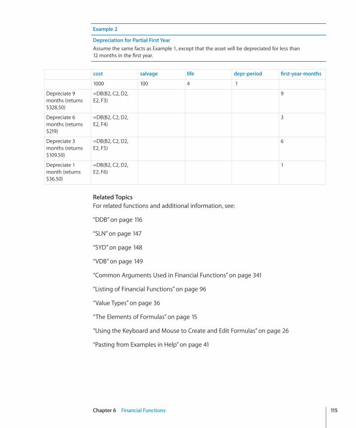
Chapter 6 Financial Functions 115
Example 2
Depreciation for Partial First YearAssume the same facts as Example 1, except that the asset will be depreciated for less than 12 months in the first year.
cost salvage life depr-period first-year-months
1000 100 4 1
Depreciate 9 months (returns $328.50)
=DB(B2, C2, D2, E2, F3)
9
Depreciate 6 months (returns $219)
=DB(B2, C2, D2, E2, F4)
3
Depreciate 3 months (returns $109.50)
=DB(B2, C2, D2, E2, F5)
6
Depreciate 1 month (returns $36.50)
=DB(B2, C2, D2, E2, F6)
1
Related TopicsFor related functions and additional information, see:
“DDB” on page 116
“SLN” on page 147
“SYD” on page 148
“VDB” on page 149
“Common Arguments Used in Financial Functions” on page 341
“Listing of Financial Functions” on page 96
“Value Types” on page 36
“The Elements of Formulas” on page 15
“Using the Keyboard and Mouse to Create and Edit Formulas” on page 26
“Pasting from Examples in Help” on page 41

DDBThe DDB function returns the amount of depreciation of an asset based on a specified depreciation rate.
DDB(cost, salvage, life, depr-period, depr-factor)
 cost:� The initial cost of the asset. cost is a number value and must be greater than or equal to 0.
 salvage:� The salvage value of the asset. salvage is a number value and must be greater than or equal to 0.
 life:� The number of periods over which the asset is depreciating. life is a number value and must be greater than 0. A decimal (fractional) part of life is allowed (for example, 5.5 for a five and one-half year depreciable life).
 depr-period:� The period for which you want to calculate depreciation. depr-period is a number value and must be greater than 0. Any decimal (fractional) part of depr-period is ignored.
 depr-factor:� An optional number that determines the depreciation rate. depr-factor is a number value. If omitted, 2 (200% for double-declining) is assumed. The higher the number, the more rapid the depreciation. For example, if a depreciation rate of one and one-half times the straight line depreciation is desired, use 1.5 or 150%.
Examples
Assume you have just purchased an asset with a cost of $1,000, a salvage value of $100, and an expected useful life of 4 years.
Using the DDB function, you can determine the depreciation for different periods and different depreciation rates.
cost salvage life depr-period depr-factor
1000 100 4
First year, double-declining balance (returns $500)
=DDB(B2, C2, D2, E3, F3)
1 2
Second year, double-declining balance (returns $250)
=DDB(B2, C2, D2, E4, F4)
2 2
Third year, double-declining balance (returns $125)
=DDB(B2, C2, D2, E5, F5)
3 2
Fourth year, double-declining balance (returns $25)
=DDB(B2, C2, D2, E6, F6)
4 2
116 Chapter 6 Financial Functions

Chapter 6 Financial Functions 117
cost salvage life depr-period depr-factor
First year, straight-line (returns $250)
=DDB(B2, C2, D2, E7, F7)
1 1
First year, triple-declining balance (returns $750)
=DDB(B2, C2, D2, E8, F8)
3 1
Related TopicsFor related functions and additional information, see:
“DB” on page 114
“SLN” on page 147
“SYD” on page 148
“VDB” on page 149
“Common Arguments Used in Financial Functions” on page 341
“Listing of Financial Functions” on page 96
“Value Types” on page 36
“The Elements of Formulas” on page 15
“Using the Keyboard and Mouse to Create and Edit Formulas” on page 26
“Pasting from Examples in Help” on page 41
DISCThe DISC function returns the annual discount rate of a security that pays no interest and is sold at a discount to its redemption value.
DISC(settle, maturity, price, redemption, days-basis)
 settle:� The trade settlement date. settle is a date/time value. The trade settlement date is usually one or more days after the trade date.
 maturity:� The date when the security matures. maturity is a date/time value. It must be after settle.
 price:� The cost of the security per $100 of par value. price is a number value.
 redemption:� The redemption value per $100 of par value. redemption is a number value that must be greater than 0. redemption is the amount that will be received per $100 of face value. Often, it is 100, meaning that the security’s redemption value is equal to its face value.

 days-basis:� An optional argument specifying the number of days per month and days per year used in the calculations.
30/360 (0 or omitted):� 30 days in a month, 360 days in a year, using the NASD method for dates falling on the 31st of a month.
actual/actual (1):� Actual days in each month, actual days in each year.
actual/360 (2):� Actual days in each month, 360 days in a year.
actual/365 (3):� Actual days in each month, 365 days in a year.
30E/360 (4):� 30 days in a month, 360 days in a year, using the European method for dates falling on the 31st of a month (European 30/360).
Example
In this example, the DISC function is used to determine the annual discount rate of the hypothetical security described by the values listed.
The function evaluates to 5.25%, the annual discount rate.
settle maturity price redemption days-basis
=DISC(B2, C2, D2, E2, F2)
05/01/2009 06/30/2015 67.64 100 0
Related TopicsFor related functions and additional information, see:
“PRICEDISC” on page 138
“YIELDDISC” on page 152
“Common Arguments Used in Financial Functions” on page 341
“Listing of Financial Functions” on page 96
“Value Types” on page 36
“The Elements of Formulas” on page 15
“Using the Keyboard and Mouse to Create and Edit Formulas” on page 26
“Pasting from Examples in Help” on page 41
118 Chapter 6 Financial Functions

Chapter 6 Financial Functions 119
EFFECTThe EFFECT function returns the effective annual interest rate from the nominal annual interest rate based on the number of compounding periods per year.
EFFECT(nominal-rate, num-periods-year)
 nominal-rate:� The nominal rate of interest of a security. nominal-rate is a number value and is either entered as a decimal (for example, 0.08) or with a percent sign (for example, 8%).
 num-periods-year:� The number of compounding periods per year. num-periods-year is a number value and must be greater than 0.
Examples
=EFFECT(0.05, 365) returns approximately 5.13%, the effective annual interest rate if 5% is compounded daily.
=EFFECT(0.05, 12) returns approximately 5.12%, the effective annual interest rate if 5% is compounded monthly.
=EFFECT(0.05, 4) returns approximately 5.09%, the effective annual interest rate if 5% is compounded quarterly.
=EFFECT(0.05, 2) returns approximately 5.06%, the effective annual interest rate if 5% is compounded semiannually.
=EFFECT(0.05, 1) returns approximately 5.00%, the effective annual interest rate if 5% is compounded annually.
Related TopicsFor related functions and additional information, see:
“NOMINAL” on page 129
“Common Arguments Used in Financial Functions” on page 341
“Listing of Financial Functions” on page 96
“Value Types” on page 36
“The Elements of Formulas” on page 15
“Using the Keyboard and Mouse to Create and Edit Formulas” on page 26
“Pasting from Examples in Help” on page 41

FVThe FV function returns the future value of an investment based on a series of regular periodic cash flows (payments of a constant amount and all cash flows at constant intervals) and a fixed interest rate.
FV(periodic-rate, num-periods, payment, present-value, when-due)
 periodic-rate:� The interest rate per period. periodic-rate is a number value and is either entered as a decimal (for example, 0.08) or with a percent sign (for example, 8%).
 num-periods:� The number of periods. num-periods is a number value and must be greater than or equal to 0.
 payment:� The payment made or amount received each period. payment is a number value. At each period, an amount received is a positive amount and an amount invested is a negative amount. For example, it could be a monthly loan payment (negative) or the periodic payment received on an annuity (positive).
 present-value:� An optional argument that specifies the value of the initial investment, or the amount of the loan or annuity. present-value is a number value. At time 0, an amount received is a positive amount and an amount invested is a negative amount. For example, it could be an amount borrowed (positive) or the initial payment made on an annuity contract (negative).
 when-due:� An optional argument that specifies whether payments are due at the beginning or end of each period. Most mortgage and other loans require the first payment at the end of the first period (0), which is the default. Most lease and rent payments, and some other types of payments, are due at the beginning of each period (1).
end (0 or omitted):� Payments are due at the end of each period.
beginning (1):� Payments are due at the beginning of each period.
Usage NotesIf  payment is specified and there is no initial investment, present-value may be omitted.
Example 1
Assume you are planning for your daughter’s college education. She has just turned 3 and you expect she will begin college in 15 years. You have $50,000 to set aside in a savings account today and can add $200 to the account at the end of each month. Over the next 15 years, the savings account is expected to earn an annual interest rate of 4.5%, and pays interest monthly.
Using the FV function, you can determine the expected value of this savings account at the time your daughter begins college. Based on the assumptions given, it would be $149,553.00.
periodic-rate num-periods payment present-value when-due
=FV(B2, C2, D2, E2, F2)
=0.045/12 =15*12 -200 -50000 1
120 Chapter 6 Financial Functions

Chapter 6 Financial Functions 121
Example 2
Assume you are presented with an investment opportunity. The opportunity requires that you invest $50,000 in a discount security today and then nothing further. The discount security matures in 14 years and has a redemption value of $100,000. Your alternative is to leave your money in your money market savings account where it is expected to earn an annual yield of 5.25%.
One way to evaluate this opportunity would be to consider how much the $50,000 would be worth at the end of the investment period and compare that to the redemption value of the security.
Using the FV function, you can determine the expected future value of the money market account. Based on the assumptions given, it would be $102,348.03. Therefore, if all assumptions happen as expected, it would be better to keep the money in the money market account since its value after 14 years ($102,348.03) exceeds the redemption value of the security ($100,000).
periodic-rate num-periods payment present-value when-due
=FV(B2, C2, D2, E2, F2)
0.0525 14 0 -50000 1
Related TopicsFor related functions and additional information, see:
“NPER” on page 130
“NPV” on page 132
“PMT” on page 134
“PV” on page 141
“RATE” on page 144
“Choosing Which Time Value of Money Function to Use” on page 348
“Common Arguments Used in Financial Functions” on page 341
“Listing of Financial Functions” on page 96
“Value Types” on page 36
“The Elements of Formulas” on page 15
“Using the Keyboard and Mouse to Create and Edit Formulas” on page 26
“Pasting from Examples in Help” on page 41

INTRATEThe INTRATE function returns the effective annual interest rate for a security that pays interest only at maturity.
INTRATE(settle, maturity, invest-amount, redemption, days-basis)
 settle:� The trade settlement date. settle is a date/time value. The trade settlement date is usually one or more days after the trade date.
 maturity:� The date when the security matures. maturity is a date/time value. It must be after settle.
 invest-amount:� The amount invested in the security. invest-amount is a number value and must be greater than or equal to 0.
 redemption:� The redemption value per $100 of par value. redemption is a number value that must be greater than 0. redemption is the amount that will be received per $100 of face value. Often, it is 100, meaning that the security’s redemption value is equal to its face value.
 days-basis:� An optional argument specifying the number of days per month and days per year used in the calculations.
30/360 (0 or omitted):� 30 days in a month, 360 days in a year, using the NASD method for dates falling on the 31st of a month.
actual/actual (1):� Actual days in each month, actual days in each year.
actual/360 (2):� Actual days in each month, 360 days in a year.
actual/365 (3):� Actual days in each month, 365 days in a year.
30E/360 (4):� 30 days in a month, 360 days in a year, using the European method for dates falling on the 31st of a month (European 30/360).
Example
In this example, the INTRATE function is used to determine the effective annual interest rate of the hypothetical security described by the values listed. The security pays interest only at maturity. The function evaluates to approximately 10.85%.
settle maturity invest-amount par days-basis
=INTRATE(B2, C2, D2, E2, F2)
05/01/2009 06/30/2015 990.02 1651.83 0
122 Chapter 6 Financial Functions

Chapter 6 Financial Functions 123
Related TopicsFor related functions and additional information, see:
“RECEIVED” on page 146
“Common Arguments Used in Financial Functions” on page 341
“Listing of Financial Functions” on page 96
“Value Types” on page 36
“The Elements of Formulas” on page 15
“Using the Keyboard and Mouse to Create and Edit Formulas” on page 26
“Pasting from Examples in Help” on page 41
IPMTThe IPMT function returns the interest portion of a specified loan or annuity payment based on fixed, periodic payments and a fixed interest rate.
IPMT(periodic-rate, period, num-periods, present-value, future-value, when-due)
 periodic-rate:� The interest rate per period. periodic-rate is a number value and is either entered as a decimal (for example, 0.08) or with a percent sign (for example, 8%).
 period:� The payment period for which you want to calculate the amount of principal or interest. period is a number and must be greater than 0.
 num-periods:� The number of periods. num-periods is a number value and must be greater than or equal to 0.
 present-value:� The value of the initial investment, or the amount of the loan or annuity. present-value is a number value. At time 0, an amount received is a positive amount and an amount invested is a negative amount. For example, it could be an amount borrowed (positive) or the initial payment made on an annuity contract (negative).
 future-value:� An optional argument that represents the value of the investment or remaining cash value of the annuity (positive amount), or the remaining loan balance (negative amount), after the final payment. future-value is a number value. At the end of the investment period, an amount received is a positive amount and an amount invested is a negative amount. For example, It could be the balloon payment due on a loan (negative) or the remaining value of an annuity contract (positive). If omitted, it is assumed to be 0.

 when-due:� An optional argument that specifies whether payments are due at the beginning or end of each period. Most mortgage and other loans require the first payment at the end of the first period (0), which is the default. Most lease and rent payments, and some other types of payments, are due at the beginning of each period (1).
end (0 or omitted):� Payments are due at the end of each period.
beginning (1):� Payments are due at the beginning of each period.
Example
In this example, IPMT is used to determine the interest portion of the first payment of the third year of the loan term (payment 25) given the loan facts presented. The function evaluates to approximately –$922.41 representing the interest portion of loan payment 25.
periodic-rate period num-periods present-value future-value when-due
=IPMT(B2, C2, D2, E2, F2, G2)
=0.06/12 25 =10*12 200000 -100000 0
Related TopicsFor related functions and additional information, see:
“CUMIPMT” on page 110
“CUMPRINC” on page 112
“PMT” on page 134
“PPMT” on page 135
“Example of a Loan Amortization Table” on page 353
“Choosing Which Time Value of Money Function to Use” on page 348
“Common Arguments Used in Financial Functions” on page 341
“Listing of Financial Functions” on page 96
“Value Types” on page 36
“The Elements of Formulas” on page 15
“Using the Keyboard and Mouse to Create and Edit Formulas” on page 26
“Pasting from Examples in Help” on page 41
124 Chapter 6 Financial Functions

Chapter 6 Financial Functions 125
IRRThe IRR function returns the internal rate of return for an investment that is based on a series of potentially irregular cash flows (payments that do not need to be a constant amount) that occur at regular time intervals.
IRR(flows-range, estimate)
 flows-range: A collection that contains the cash flow values. flows-range is a collection containing number values. Income (a cash inflow) is specified as a positive number, and an expenditure (a cash outflow) is specified as a negative number. There must be at least one positive and one negative value included within the collection. Cash flows must be specified in chronological order and equally spaced in time (for example, each month). If a period does not have a cash flow, use 0 for that period.
 estimate:� An optional argument specifying the initial estimate for the rate of return. estimate is a number value and is either entered as a decimal (for example, 0.08) or with a percent sign (for example, 8%). If omitted, 10% is assumed. If the default value does not result in a solution, initially try a larger positive value. If this does not result in an outcome, try a small negative value. The minimum value allowed is –1.
Usage NotesIf the periodic cash flows are the same, consider using the NPV function. Â
Example 1
Assume you are planning for your daughter’s college education. She has just turned 13 and you expect she will begin college in 5 years. You have $75,000 to set aside in a savings account today and will add the bonus you receive from your employer at the end of each year. Since you expect your bonus to increase each year, you expect to be able to set aside $5,000, $7,000, $8,000, $9,000, and $10,000, respectively, at the end of each of the next 5 years. You think you will need to have $150,000 set aside for her education by the time your daughter reaches college.
Using the IRR function, you can determine the rate you would need to receive on invested amounts in order to have $150,000. Based on the assumptions given, the rate would be 5.70%.
Initial Deposit
Year 1 Year 2 Year 3 Year 4 Year 5 Amount Required
=IRR(B2:H2) -75000 -5000 -7000 -8000 -9000 -10000 150000

Example 2
Assume you are presented with the opportunity to invest in a partnership. The initial investment required is $50,000. Because the partnership is still developing its product, an additional $25,000 and $10,000 must be invested at the end of the first and second years, respectively. In the third year the partnership expects to be self-funding but not return any cash to investors. In the fourth and fifth years, investors are projected to receive $10,000 and $30,000, respectively. At the end of the sixth year, the company expects to sell and investors are projected to receive $100,000.
Using the IRR function, you can determine the expected rate of return on this investment. Based on the assumptions given, the rate would be 10.24%.
Initial Deposit
Year 1 Year 2 Year 3 Year 4 Year 5 Sales proceeds
=IRR(B2:H2) -50000 -25000 -10000 0 10000 30000 100000
Related TopicsFor related functions and additional information, see:
“MIRR” on page 128
“NPV” on page 132
“Choosing Which Time Value of Money Function to Use” on page 348
“Common Arguments Used in Financial Functions” on page 341
“Listing of Financial Functions” on page 96
“Value Types” on page 36
“The Elements of Formulas” on page 15
“Using the Keyboard and Mouse to Create and Edit Formulas” on page 26
“Pasting from Examples in Help” on page 41
ISPMTThe ISPMT function returns the interest portion of a specified loan or annuity payment based on fixed, periodic payments and a fixed interest rate. This function is provided for compatibility with tables imported from other spreadsheet applications.
126 Chapter 6 Financial Functions

Chapter 6 Financial Functions 127
ISPMT(annual-rate, period, num-periods, present-value)
 annual-rate:� The annual coupon rate or stated annual interest rate of the security. annual-rate is a number value and is either entered as a decimal (for example, 0.08) or with a percent sign (for example, 8%).
 period:� The payment period for which you want to calculate the amount of principal or interest. period is a number and must be greater than 0.
 num-periods:� The number of periods. num-periods is a number value and must be greater than or equal to 0.
 present-value:� The value of the initial investment, or the amount of the loan or annuity. present-value is a number value. At time 0, an amount received is a positive amount and an amount invested is a negative amount. For example, it could be an amount borrowed (positive) or the initial payment made on an annuity contract (negative).
Usage NotesThe IPMT function has additional functionality and should be used instead of ISPMT. Â
Example
In this example, ISPMT is used to determine the interest portion of the first payment of the third year of the loan term (payment 25) given the loan facts presented.
The function evaluates to approximately –$791.67, which represents the interest portion of loan payment 25.
periodic-rate period num-periods present-value
=ISPMT(B2, C2, D2, E2) =0.06/12 25 =10*12 200000
Related TopicsFor related functions and additional information, see:
“IPMT” on page 123
“Common Arguments Used in Financial Functions” on page 341
“Listing of Financial Functions” on page 96
“Value Types” on page 36
“The Elements of Formulas” on page 15
“Using the Keyboard and Mouse to Create and Edit Formulas” on page 26
“Pasting from Examples in Help” on page 41

MIRRThe MIRR function returns the modified internal rate of return for an investment that is based on a series of potentially irregular cash flows (payments that do not need to be a constant amount) that occur at regular time intervals. The rate earned on positive cash flows and the rate paid to finance negative cash flows can differ.
MIRR(flows-range, finance-rate, reinvest-rate)
 flows-range: A collection that contains the cash flow values. flows-range is a collection containing number values. Income (a cash inflow) is specified as a positive number, and an expenditure (a cash outflow) is specified as a negative number. There must be at least one positive and one negative value included within the collection. Cash flows must be specified in chronological order and equally spaced in time (for example, each month). If a period does not have a cash flow, use 0 for that period.
 finance-rate: Interest rate paid on negative cash flows (outflows). finance-rate is a number value and is either entered as a decimal (for example, 0.08) or with a percent sign (for example, 8%) and represents the rate at which the amounts invested (negative cash flows) can be financed. For example, a company’s cost of capital might be used.
 reinvest-rate:� Rate at which positive cash flows (inflows) can be reinvested. reinvest-rate is a number value and is either entered as a decimal (for example, 0.08) or with a percent sign (for example, 8%) and represents the rate at which the amounts received (positive cash flows) can be reinvested. For example, a company’s short-term investment rate might be used.
Usage NotesCash flows must be equally spaced in time. If there is no cash flow in a particular Âtime period, use 0.
Example 1
Assume you are presented with the opportunity to invest in a partnership. The initial investment required is $50,000. Because the partnership is still developing its product, an additional $25,000 and $10,000 must be invested at the end of the first and second years, respectively. In the third year the partnership expects to be self-funding but not return any cash to investors. In the fourth and fifth years, investors are projected to receive $10,000 and $30,000, respectively. At the end of the sixth year, the company expects to sell and investors are projected to receive $100,000. Assume that you can currently borrow money at 9.00% (finance-rate) and can earn 4.25% on short-term savings (reinvest-rate).
Using the IRR function, you can determine the expected rate of return on this investment. Based on the assumptions given, the rate would be approximately 9.75%.
128 Chapter 6 Financial Functions

Chapter 6 Financial Functions 129
Initial Deposit
Year 1 Year 2 Year 3 Year 4 Year 5 Sales proceeds
=MIRR (B2:H2, 0.09, 0.0425)
-50000 -25000 -10000 0 10000 30000 100000
Example 2
Assume the same information as in Example 1, but rather than placing the cash flows in individual cells, you specify the cash flows as an array constant. The MIRR function would then be as follows:
=MIRR({-50000, -25000, -10000, 0, 10000, 30000, 100000}, 0.09, 0.0425) returns approximately 9.75%.
Related TopicsFor related functions and additional information, see:
“IRR” on page 125
“NPV” on page 132
“PV” on page 141
“Choosing Which Time Value of Money Function to Use” on page 348
“Common Arguments Used in Financial Functions” on page 341
“Listing of Financial Functions” on page 96
“Value Types” on page 36
“The Elements of Formulas” on page 15
“Using the Keyboard and Mouse to Create and Edit Formulas” on page 26
“Pasting from Examples in Help” on page 41
NOMINALThe NOMINAL function returns the nominal annual interest rate from the effective annual interest rate based on the number of compounding periods per year.
NOMINAL(effective-int-rate, num-periods-year)
 effective-int-rate: The effective interest rate of a security. effective-int-rate is a number value and is either entered as a decimal (for example, 0.08) or with a percent sign (for example, 8%).
 num-periods-year:� The number of compounding periods per year. num-periods-year is a number value and must be greater than 0.

Examples
=NOMINAL(0.0513, 365) returns approximately 5.00%, the nominal annual interest rate if the effective rate of 5.13% was based on daily compounding.
=NOMINAL(0.0512, 12) returns approximately 5.00%, the nominal annual interest rate if the effective rate of 5.12% was based on monthly compounding.
=NOMINAL(0.0509, 4) returns approximately 5.00%, the nominal annual interest rate if the effective rate of 5.09% was based on quarterly compounding.
=NOMINAL(0.0506, 2) returns approximately 5.00%, the nominal annual interest rate if the effective rate of 5.06% was based on semiannual compounding.
=NOMINAL(0.0500, 1) returns approximately 5.00%, the nominal annual interest rate if the effective rate of 5.00% was based on annual compounding.
Related TopicsFor related functions and additional information, see:
“EFFECT” on page 119
“Common Arguments Used in Financial Functions” on page 341
“Listing of Financial Functions” on page 96
“Value Types” on page 36
“The Elements of Formulas” on page 15
“Using the Keyboard and Mouse to Create and Edit Formulas” on page 26
“Pasting from Examples in Help” on page 41
NPERThe NPER function returns the number of payment periods for a loan or annuity based on a series of regular periodic cash flows (payments of a constant amount and all cash flows at constant intervals) and a fixed interest rate.
NPER(periodic-rate, payment, present-value, future-value, when-due)
 periodic-rate:� The interest rate per period. periodic-rate is a number value and is either entered as a decimal (for example, 0.08) or with a percent sign (for example, 8%).
 payment:� The payment made or amount received each period. payment is a number value. At each period, an amount received is a positive amount and an amount invested is a negative amount. For example, it could be a monthly loan payment (negative) or the periodic payment received on an annuity (positive).
130 Chapter 6 Financial Functions

Chapter 6 Financial Functions 131
 present value:� The value of the initial investment, or the amount of the loan or annuity, specified as a negative number. present-value is a number value. At time 0, an amount received is a positive amount and an amount invested is a negative amount. For example, It could be an amount borrowed (positive) or the initial payment made on an annuity contract (negative).
 future-value:� An optional argument specifying the value of the investment or remaining cash value of the annuity (positive amount), or the remaining loan balance (negative amount), after the final payment. future-value is a number value. At the end of the investment period, an amount received is a positive amount and an amount invested is a negative amount. For example, It could be the balloon payment due on a loan (negative) or the remaining value of an annuity contract (positive).
 when-due:� An optional argument that specifies whether payments are due at the beginning or end of each period. Most mortgage and other loans require the first payment at the end of the first period (0), which is the default. Most lease and rent payments, and some other types of payments, are due at the beginning of each period (1).
end (0 or omitted):� Payments are due at the end of each period.
beginning (1):� Payments are due at the beginning of each period.
Example 1
Assume you are planning for your daughter’s college education. You have $50,000 to set aside in a savings account today and can add $200 to the account at the end of each month. The savings account is expected to earn an annual interest rate of 4.5%, and pays interest monthly. You believe you will need to have set aside $150,000 by the time your daughter reaches college.
Using the NPER function, you can determine the number of periods you would need to make the $200 payment. Based on the assumptions given, it would be approximately 181 periods or 15 years, 1 month.
periodic-rate payment present-value future-value when-due
=NPER(B2, C2, D2, E2, F2)
=0.045/12 -200 -50000 150000 1
Example 2
Assume you are planning to purchase your uncle’s mountain cabin. You have $30,000 to use as a down payment today and can afford to make a monthly payment of $1,500. Your uncle says he is willing to lend you the difference between the cabin’s sale price of $200,000 and your down payment (so you would borrow $170,000) at an annual rate of 7%.
Using the NPER function, you can determine the number of months it would take you to repay your uncle’s loan. Based on the assumptions given, it would be approximately 184 months or 15 years, 4 months.

periodic-rate payment present-value future-value when-due
=NPER(B2, C2, D2, E2, F2)
=0.07/12 -1500 170000 0 1
Related TopicsFor related functions and additional information, see:
“FV” on page 120
“PMT” on page 134
“PV” on page 141
“RATE” on page 144
“Choosing Which Time Value of Money Function to Use” on page 348
“Common Arguments Used in Financial Functions” on page 341
“Listing of Financial Functions” on page 96
“Value Types” on page 36
“The Elements of Formulas” on page 15
“Using the Keyboard and Mouse to Create and Edit Formulas” on page 26
“Pasting from Examples in Help” on page 41
NPVThe NPV function returns the net present value of an investment based on a series of potentially irregular cash flows that occur at regular time intervals.
NPV(periodic-discount-rate, cash-flow, cash-flow…)
 periodic-discount-rate:� The discount rate per period. periodic-discount-rate is a number value and is either entered as a decimal (for example, 0.08) or with a percent sign (for example, 8%). periodic-discount-rate must be greater than or equal to 0.
 cash-flow: A cash flow. cash-flow is a number value. A positive value represents income (cash inflow). A negative value represents an expenditure (cash outflow). Cash flows must be equally spaced in time.
 cash-flow…: Optionally include one or more additional cash flows.
132 Chapter 6 Financial Functions

Chapter 6 Financial Functions 133
Usage Notes  periodic-discount-rate is specified using the same time frame as the time frame used
for the cash flows. For example, if the cash flows are monthly and the desired annual discount rate is 8%, periodic-discount-rate must be specified as 0.00667 or 0.667% (0.08 divided by 12).
If cash flows are irregular, use the IRR function. Â
Example
Assume you are presented with the opportunity to invest in a partnership. Because the partnership is still developing its product, an additional $25,000 and $10,000 must be invested at the end of the first and second years, respectively. In the third year the partnership expects to be self-funding but not return any cash to investors. In the fourth and fifth years, investors are projected to receive $10,000 and $30,000, respectively. At the end of the sixth year, the company expects to sell and investors are projected to receive $100,000. In order to invest, you want to achieve an annual return of at least 10%.
Using the NPV function, you can determine the maximum amount you are willing to initially invest. Based on the assumptions given, the NPV would be $50,913.43. Therefore if the required initial investment is this amount or less, this opportunity meets your 10% goal.
periodic-rate Year 1 Year 2 Year 3 Year 4 Year 5 Sales proceeds
=NPV(B2, C2:H2)
0.10 -25000 -10000 0 10000 30000 100000
Related TopicsFor related functions and additional information, see:
“IRR” on page 125
“PV” on page 141
“Choosing Which Time Value of Money Function to Use” on page 348
“Common Arguments Used in Financial Functions” on page 341
“Listing of Financial Functions” on page 96
“Value Types” on page 36
“The Elements of Formulas” on page 15
“Using the Keyboard and Mouse to Create and Edit Formulas” on page 26
“Pasting from Examples in Help” on page 41

PMTThe PMT function returns the fixed periodic payment for a loan or annuity based on a series of regular periodic cash flows (payments of a constant amount and all cash flows at constant intervals) and a fixed interest rate.
PMT(periodic-rate, num-periods, present-value, future-value, when-due)
 periodic-rate:� The interest rate per period. periodic-rate is a number value and is either entered as a decimal (for example, 0.08) or with a percent sign (for example, 8%).
 num-periods:� The number of periods. num-periods is a number value and must be greater than or equal to 0.
 present-value:� The value of the initial investment, or the amount of the loan or annuity. present-value is a number value. At time 0, an amount received is a positive amount and an amount invested is a negative amount. For example, it could be an amount borrowed (positive) or the initial payment made on an annuity contract (negative).
 future-value:� An optional argument that represents the value of the investment or remaining cash value of the annuity (positive amount), or the remaining loan balance (negative amount), after the final payment. future-value is a number value. At the end of the investment period, an amount received is a positive amount and an amount invested is a negative amount. For example, It could be the balloon payment due on a loan (negative) or the remaining value of an annuity contract (positive). If omitted, it is assumed to be 0.
 when-due:� An optional argument that specifies whether payments are due at the beginning or end of each period. Most mortgage and other loans require the first payment at the end of the first period (0), which is the default. Most lease and rent payments, and some other types of payments, are due at the beginning of each period (1).
end (0 or omitted):� Payments are due at the end of each period.
beginning (1):� Payments are due at the beginning of each period.
Example
In this example, PMT is used to determine the fixed payment given the loan facts presented.
The function evaluates to –$1,610.21, which represents the fixed payment you would make (negative because it is a cash outflow) for this loan.
periodic-rate num-periods present-value future-value when-due
=PMT(B2, C2, D2, E2, F2)
=0.06/12 =10*12 200000 -100000 0
134 Chapter 6 Financial Functions

Chapter 6 Financial Functions 135
Related TopicsFor related functions and additional information, see:
“FV” on page 120
“IPMT” on page 123
“NPER” on page 130
“PPMT” on page 135
“PV” on page 141
“RATE” on page 144
“Example of a Loan Amortization Table” on page 353
“Choosing Which Time Value of Money Function to Use” on page 348
“Common Arguments Used in Financial Functions” on page 341
“Listing of Financial Functions” on page 96
“Value Types” on page 36
“The Elements of Formulas” on page 15
“Using the Keyboard and Mouse to Create and Edit Formulas” on page 26
“Pasting from Examples in Help” on page 41
PPMTThe PPMT function returns the principal portion of a specified loan or annuity payment based on fixed periodic payments and a fixed interest rate.
PPMT(periodic-rate, period, num-periods, present-value, future-value, when-due)
 periodic-rate:� The interest rate per period. periodic-rate is a number value and is either entered as a decimal (for example, 0.08) or with a percent sign (for example, 8%).
 period:� The payment period for which you want to calculate the amount of principal or interest. period is a number and must be greater than 0.
 num-periods:� The number of periods. num-periods is a number value and must be greater than or equal to 0.

 present-value:� The value of the initial investment, or the amount of the loan or annuity. present-value is a number value. At time 0, an amount received is a positive amount and an amount invested is a negative amount. For example, it could be an amount borrowed (positive) or the initial payment made on an annuity contract (negative).
 future-value:� An optional argument that represents the value of the investment or remaining cash value of the annuity (positive amount), or the remaining loan balance (negative amount), after the final payment. future-value is a number value. At the end of the investment period, an amount received is a positive amount and an amount invested is a negative amount. For example, It could be the balloon payment due on a loan (negative) or the remaining value of an annuity contract (positive). If omitted, it is assumed to be 0.
 when-due:� An optional argument that specifies whether payments are due at the beginning or end of each period. Most mortgage and other loans require the first payment at the end of the first period (0), which is the default. Most lease and rent payments, and some other types of payments, are due at the beginning of each period (1).
end (0 or omitted):� Payments are due at the end of each period.
beginning (1):� Payments are due at the beginning of each period.
Example
In this example, PPMT is used to determine the principal portion of the first payment of the third year of the loan term (payment 25) given the loan facts presented. The function evaluates to approximately –$687.80, which represents the principal portion of payment 25.
periodic-rate period num-periods present-value future-value when-due
=PPMT(B2, C2, D2, E2, F2, G2)
=0.06/12 25 =10*12 200000 -100000 0
Related TopicsFor related functions and additional information, see:
“CUMIPMT” on page 110
“CUMPRINC” on page 112
“IPMT” on page 123
“PMT” on page 134
“Example of a Loan Amortization Table” on page 353
“Choosing Which Time Value of Money Function to Use” on page 348
“Common Arguments Used in Financial Functions” on page 341
136 Chapter 6 Financial Functions

Chapter 6 Financial Functions 137
“Listing of Financial Functions” on page 96
“Value Types” on page 36
“The Elements of Formulas” on page 15
“Using the Keyboard and Mouse to Create and Edit Formulas” on page 26
“Pasting from Examples in Help” on page 41
PRICEThe PRICE function returns the price of a security that pays periodic interest per $100 of redemption (par) value.
PRICE(settle, maturity, annual-rate, annual-yield, redemption, frequency, days-basis)
 settle:� The trade settlement date. settle is a date/time value. The trade settlement date is usually one or more days after the trade date.
 maturity:� The date when the security matures. maturity is a date/time value. It must be after settle.
 annual-rate:� The annual coupon rate or stated annual interest rate of the security. annual-rate is a number value and is either entered as a decimal (for example, 0.08) or with a percent sign (for example, 8%).
 annual-yield:� The annual yield of the security. annual-yield is a number value and is either entered as a decimal (for example, 0.08) or with a percent sign (for example, 8%).
 redemption:� The redemption value per $100 of par value. redemption is a number value that must be greater than 0. redemption is the amount that will be received per $100 of face value. Often, it is 100, meaning that the security’s redemption value is equal to its face value.
 frequency:� The number of coupon payments each year.
annual (1):� One payment per year.
semiannual (2):� Two payments per year.
quarterly (4):� Four payments per year.
 days-basis:� An optional argument specifying the number of days per month and days per year used in the calculations.
30/360 (0 or omitted):� 30 days in a month, 360 days in a year, using the NASD method for dates falling on the 31st of a month.
actual/actual (1):� Actual days in each month, actual days in each year.
actual/360 (2):� Actual days in each month, 360 days in a year.
actual/365 (3):� Actual days in each month, 365 days in a year.

30E/360 (4):� 30 days in a month, 360 days in a year, using the European method for dates falling on the 31st of a month (European 30/360).
Example
In this example, the PRICE function is used to determine the purchase price when trading the hypothetical security described by the values listed. The security pays periodic interest.
The function evaluates to $106.50, which represents the price per $100 of face value.
settle maturity annual-rate annual-yield redemption frequency days-basis
=PRICE (B2, C2, D2, E2, F2, G2, H2)
05/01/2009 06/30/2015 0.065 0.0525 100 2 0
Related TopicsFor related functions and additional information, see:
“PRICEDISC” on page 138
“PRICEMAT” on page 140
“YIELD” on page 150
“Common Arguments Used in Financial Functions” on page 341
“Listing of Financial Functions” on page 96
“Value Types” on page 36
“The Elements of Formulas” on page 15
“Using the Keyboard and Mouse to Create and Edit Formulas” on page 26
“Pasting from Examples in Help” on page 41
PRICEDISCThe PRICEDISC function returns the price of a security that is sold at a discount to redemption value and does not pay interest per $100 of redemption (par) value.
PRICEDISC(settle, maturity, annual-yield, redemption, days-basis)
 settle:� The trade settlement date. settle is a date/time value. The trade settlement date is usually one or more days after the trade date.
 maturity:� The date when the security matures. maturity is a date/time value. It must be after settle.
 annual-yield:� The annual yield of the security. annual-yield is a number value and is either entered as a decimal (for example, 0.08) or with a percent sign (for example, 8%).
138 Chapter 6 Financial Functions

Chapter 6 Financial Functions 139
 redemption:� The redemption value per $100 of par value. redemption is a number value that must be greater than 0. redemption is the amount that will be received per $100 of face value. Often, it is 100, meaning that the security’s redemption value is equal to its face value.
 days-basis:� An optional argument specifying the number of days per month and days per year used in the calculations.
30/360 (0 or omitted):� 30 days in a month, 360 days in a year, using the NASD method for dates falling on the 31st of a month.
actual/actual (1):� Actual days in each month, actual days in each year.
actual/360 (2):� Actual days in each month, 360 days in a year.
actual/365 (3):� Actual days in each month, 365 days in a year.
30E/360 (4):� 30 days in a month, 360 days in a year, using the European method for dates falling on the 31st of a month (European 30/360).
Example
In this example, the PRICEDISC function is used to determine the purchase price when trading the hypothetical security described by the values listed. The security does not pay interest and is sold at a discount.
The function evaluates to approximately $65.98, which represents the price per $100 of face value.
settle maturity discount redemption days-basis
=PRICEDISC (B2, C2, D2, E2, F2)
05/01/2009 06/30/2015 0.0552 100 0
Related TopicsFor related functions and additional information, see:
“PRICE” on page 137
“PRICEMAT” on page 140
“YIELDDISC” on page 152
“Common Arguments Used in Financial Functions” on page 341
“Listing of Financial Functions” on page 96
“Value Types” on page 36
“The Elements of Formulas” on page 15
“Using the Keyboard and Mouse to Create and Edit Formulas” on page 26
“Pasting from Examples in Help” on page 41

PRICEMATThe PRICEMAT function returns the price of a security that pays interest only at maturity per $100 of redemption (par) value.
PRICEMAT(settle, maturity, issue, annual-rate, annual-yield, days-basis)
 settle:� The trade settlement date. settle is a date/time value. The trade settlement date is usually one or more days after the trade date.
 maturity:� The date when the security matures. maturity is a date/time value. It must be after settle.
 issue:� The date the security was originally issued. issue is a date/time value and must be the earliest date given.
 annual-rate:� The annual coupon rate or stated annual interest rate of the security. annual-rate is a number value and is either entered as a decimal (for example, 0.08) or with a percent sign (for example, 8%).
 annual-yield:� The annual yield of the security. annual-yield is a number value and is either entered as a decimal (for example, 0.08) or with a percent sign (for example, 8%).
 days-basis:� An optional argument specifying the number of days per month and days per year used in the calculations.
30/360 (0 or omitted):� 30 days in a month, 360 days in a year, using the NASD method for dates falling on the 31st of a month.
actual/actual (1):� Actual days in each month, actual days in each year.
actual/360 (2):� Actual days in each month, 360 days in a year.
actual/365 (3):� Actual days in each month, 365 days in a year.
30E/360 (4):� 30 days in a month, 360 days in a year, using the European method for dates falling on the 31st of a month (European 30/360).
Example
In this example, the PRICEMAT function is used to determine the purchase price when trading the hypothetical security described by the values listed. The security pays interest only at maturity. The function evaluates to $99.002, which represents the price per $100 of face value.
settle maturity issue annual-rate annual-yield days-basis
=PRICEMAT (B2, C2, D2, E2, F2, G2)
05/01/2009 06/30/2015 12/14/2008 0.065 0.06565 0
140 Chapter 6 Financial Functions

Chapter 6 Financial Functions 141
Related TopicsFor related functions and additional information, see:
“PRICE” on page 137
“PRICEDISC” on page 138
“YIELDMAT” on page 153
“Common Arguments Used in Financial Functions” on page 341
“Listing of Financial Functions” on page 96
“Value Types” on page 36
“The Elements of Formulas” on page 15
“Using the Keyboard and Mouse to Create and Edit Formulas” on page 26
“Pasting from Examples in Help” on page 41
PVThe PV function returns the present value of an investment or annuity based on a series of regular periodic cash flows (payments of a constant amount and all cash flows at constant intervals) and a fixed interest rate.
PV(periodic-rate, num-periods, payment, future-value, when-due)
 periodic-rate:� The interest rate per period. periodic-rate is a number value and is either entered as a decimal (for example, 0.08) or with a percent sign (for example, 8%).
 num-periods:� The number of periods. num-periods is a number value and must be greater than or equal to 0.
 payment:� The payment made or amount received each period. payment is a number value. At each period, an amount received is a positive amount and an amount invested is a negative amount. For example, it could be a monthly loan payment (negative) or the periodic payment received on an annuity (positive).
 future-value:� An optional argument specifying the value of the investment or remaining cash value of the annuity (positive amount), or the remaining loan balance (negative amount), after the final payment. future-value is a number value. At the end of the investment period, an amount received is a positive amount and an amount invested is a negative amount. For example, It could be the balloon payment due on a loan (negative) or the remaining value of an annuity contract (positive).

 when-due:� An optional argument that specifies whether payments are due at the beginning or end of each period. Most mortgage and other loans require the first payment at the end of the first period (0), which is the default. Most lease and rent payments, and some other types of payments, are due at the beginning of each period (1).
end (0 or omitted):� Payments are due at the end of each period.
beginning (1):� Payments are due at the beginning of each period.
Usage Notes  periodic-rate is specified using the time frame of num-periods. For example, if num-
periods represents months and the annual interest rate is 8%, periodic-rate must be specified as 0.00667 or 0.667% (0.08 divided by 12).
If  payment is specified and there is no investment value, cash value, or loan balance remaining, future-value may be omitted.
If  payment is omitted, you must include future-value.
Example 1
Assume you are planning for your daughter’s college education. She has just turned 3 and you expect she will begin college in 15 years. You think you will need to have $150,000 set aside in a savings account by the time she reaches college. You can add $200 to the account at the end of each month. Over the next 15 years, the savings account is expected to earn an annual interest rate of 4.5%, and earns interest monthly.
Using the PV function, you can determine the amount that must be deposited to this savings account today so that the value of the savings account will reach $150,000 by the time your daughter begins college. Based on the assumptions given, the function returns –$50,227.88 as the amount that would need to be deposited today (function returns a negative because the deposit to the savings account today is a cash outflow).
periodic-rate num-periods payment future-value when-due
=PV(B2, C2, D2, E2, F2)
=0.045/12 =15*12 -200 150000 1
142 Chapter 6 Financial Functions

Chapter 6 Financial Functions 143
Example 2
In this example, you are presented with an investment opportunity. The opportunity is to invest in a discount security today and then pay or receive nothing further until the security matures. The discount security matures in 14 years and has a redemption value of $100,000. Your alternative is to leave your money in your money market savings account where it is expected to earn an annual yield of 5.25%.
Using the PV function, you can determine the maximum amount you should be willing to pay for this discount security today, assuming you want at least as good an interest rate as you expect to get on your money market account. Based on the assumptions given, it would be –$48,852.92 (the function returns a negative amount since this is a cash outflow).
periodic-rate num-periods payment future-value when-due
=PV(B2, C2, D2, E2, F2)
0.0525 14 0 100000 1
Related TopicsFor related functions and additional information, see:
“FV” on page 120
“IRR” on page 125
“NPER” on page 130
“PMT” on page 134
“RATE” on page 144
“Choosing Which Time Value of Money Function to Use” on page 348
“Common Arguments Used in Financial Functions” on page 341
“Listing of Financial Functions” on page 96
“Value Types” on page 36
“The Elements of Formulas” on page 15
“Using the Keyboard and Mouse to Create and Edit Formulas” on page 26
“Pasting from Examples in Help” on page 41

RATEThe RATE function returns the interest rate of an investment, loan, or annuity based on a series of regular periodic cash flows (payments of a constant amount and all cash flows at constant intervals) and a fixed interest rate.
RATE(num-periods, payment, present-value, future-value, when-due, estimate)
 num-periods:� The number of periods. num-periods is a number value and must be greater than or equal to 0.
 payment:� The payment made or amount received each period. payment is a number value. At each period, an amount received is a positive amount and an amount invested is a negative amount. For example, it could be a monthly loan payment (negative) or the periodic payment received on an annuity (positive).
 present-value:� The value of the initial investment, or the amount of the loan or annuity. present-value is a number value. At time 0, an amount received is a positive amount and an amount invested is a negative amount. For example, it could be an amount borrowed (positive) or the initial payment made on an annuity contract (negative).
 future-value:� An optional argument that represents the value of the investment or remaining cash value of the annuity (positive amount), or the remaining loan balance (negative amount), after the final payment. future-value is a number value. At the end of the investment period, an amount received is a positive amount and an amount invested is a negative amount. For example, It could be the balloon payment due on a loan (negative) or the remaining value of an annuity contract (positive).
 when-due:� An optional argument that specifies whether payments are due at the beginning or end of each period. Most mortgage and other loans require the first payment at the end of the first period (0), which is the default. Most lease and rent payments, and some other types of payments, are due at the beginning of each period (1).
end (0 or omitted):� Payments are due at the end of each period.
beginning (1):� Payments are due at the beginning of each period.
 estimate:� An optional argument specifying the initial estimate for the rate of return. estimate is a number value and is either entered as a decimal (for example, 0.08) or with a percent sign (for example, 8%). If omitted, 10% is assumed. If the default value does not result in a solution, initially try a larger positive value. If this does not result in an outcome, try a small negative value. The minimum value allowed is –1.
144 Chapter 6 Financial Functions

Chapter 6 Financial Functions 145
Example
Assume you are planning for your daughter’s college education. She has just turned 3 and you expect she will begin college in 15 years. You think you will need to have $150,000 set aside in a savings account by the time she reaches college. You can set aside $50,000 today and add $200 to the account at the end of each month. Over the next 15 years, the savings account is expected to earn an annual interest rate of 4.5%, and earns interest monthly.
Using the RATE function, you can determine the rate that must be earned on the savings account so that it will reach $150,000 by the time your daughter begins college. Based on the assumptions given, the rate returned by the function is approximately 0.377%, which is per month since num-periods was monthly, or 4.52% annually.
num-periods payment present-value future-value when-due estimate
=RATE(B2, C2, D2, E2, F2, G2)
=15*12 -200 -50000 150000 1 =0.1/12
Related TopicsFor related functions and additional information, see:
“FV” on page 120
“IRR” on page 125
“NPER” on page 130
“PMT” on page 134
“PV” on page 141
“Choosing Which Time Value of Money Function to Use” on page 348
“Common Arguments Used in Financial Functions” on page 341
“Listing of Financial Functions” on page 96
“Value Types” on page 36
“The Elements of Formulas” on page 15
“Using the Keyboard and Mouse to Create and Edit Formulas” on page 26
“Pasting from Examples in Help” on page 41

RECEIVEDThe RECEIVED function returns the maturity value for a security that pays interest only at maturity.
RECEIVED(settle, maturity, invest-amount, annual-rate, days-basis)
 settle:� The trade settlement date. settle is a date/time value. The trade settlement date is usually one or more days after the trade date.
 maturity:� The date when the security matures. maturity is a date/time value. It must be after settle.
 invest-amount:� The amount invested in the security. invest-amount is a number value and must be greater than or equal to 0.
 annual-rate:� The annual coupon rate or stated annual interest rate of the security. annual-rate is a number value and is either entered as a decimal (for example, 0.08) or with a percent sign (for example, 8%).
 days-basis:� An optional argument specifying the number of days per month and days per year used in the calculations.
30/360 (0 or omitted):� 30 days in a month, 360 days in a year, using the NASD method for dates falling on the 31st of a month.
actual/actual (1):� Actual days in each month, actual days in each year.
actual/360 (2):� Actual days in each month, 360 days in a year.
actual/365 (3):� Actual days in each month, 365 days in a year.
30E/360 (4):� 30 days in a month, 360 days in a year, using the European method for dates falling on the 31st of a month (European 30/360).
Example
In this example, the RECEIVED function is used to determine the amount received at the maturity of the hypothetical security described by the values listed. The security pays interest only at maturity. The function evaluates to $1,651.83, the amount to be received at maturity including both principal and interest.
settle maturity invest-amount annual-rate days-basis
=RECEIVED (B2, C2, D2, E2, F2)
05/01/2009 06/30/2015 990.02 0.065 0
Related TopicsFor related functions and additional information, see:
“INTRATE” on page 122
“Common Arguments Used in Financial Functions” on page 341
“Listing of Financial Functions” on page 96
146 Chapter 6 Financial Functions

Chapter 6 Financial Functions 147
“Value Types” on page 36
“The Elements of Formulas” on page 15
“Using the Keyboard and Mouse to Create and Edit Formulas” on page 26
“Pasting from Examples in Help” on page 41
SLNThe SLN function returns the depreciation of an asset for a single period using the straight-line method.
SLN(cost, salvage, life)
 cost:� The initial cost of the asset. cost is a number value and must be greater than or equal to 0.
 salvage:� The salvage value of the asset. salvage is a number value and must be greater than or equal to 0.
 life:� The number of periods over which the asset is depreciating. life is a number value and must be greater than 0. A decimal (fractional) part of life is allowed (for example, 5.5 for a five and one-half year depreciable life).
Example
=SLN(10000, 1000, 6) returns $1500, the depreciation per year, in dollars, of an asset that originally costs $10,000 and has an estimated salvage value of $1,000 after 6 years.
Related TopicsFor related functions and additional information, see:
“DB” on page 114
“DDB” on page 116
“SYD” on page 148
“VDB” on page 149
“Common Arguments Used in Financial Functions” on page 341
“Listing of Financial Functions” on page 96
“Value Types” on page 36
“The Elements of Formulas” on page 15
“Using the Keyboard and Mouse to Create and Edit Formulas” on page 26
“Pasting from Examples in Help” on page 41

SYDThe SYD function returns the amount of depreciation of an asset for a specified period using the sum-of-the-years-digits method.
SYD(cost, salvage, life, depr-period)
 cost:� The initial cost of the asset. cost is a number value and must be greater than or equal to 0.
 salvage:� The salvage value of the asset. salvage is a number value and must be greater than or equal to 0.
 life:� The number of periods over which the asset is depreciating. life is a number value and must be greater than 0. A decimal (fractional) part of life is allowed (for example, 5.5 for a five and one-half year depreciable life).
 depr-period:� The period for which you want to calculate depreciation. depr-period is a number value and must be greater than 0. Any decimal (fractional) part of depr-period is ignored.
Examples
=SYD(10000, 1000, 9, 1) returns $1,800, the depreciation amount for the first year for an asset with an initial cost of $10,000 and a salvage value of $1,000 after a 9-year life.
=SYD(10000, 1000, 9, 2) returns $1,600, the depreciation amount for the second year.
=SYD(10000, 1000, 9, 8) returns $400, the depreciation amount for the eighth year.
Related TopicsFor related functions and additional information, see:
“DB” on page 114
“DDB” on page 116
“SLN” on page 147
“VDB” on page 149
“Common Arguments Used in Financial Functions” on page 341
“Listing of Financial Functions” on page 96
“Value Types” on page 36
“The Elements of Formulas” on page 15
“Using the Keyboard and Mouse to Create and Edit Formulas” on page 26
“Pasting from Examples in Help” on page 41
148 Chapter 6 Financial Functions

Chapter 6 Financial Functions 149
VDBThe VDB (variable declining balance) function returns the amount of depreciation of an asset over a chosen time interval, based on a specified depreciation rate.
VDB(cost, salvage, life, starting-per, ending-per, depr-factor, no-switch)
 cost:� The initial cost of the asset. cost is a number value and must be greater than or equal to 0.
 salvage:� The salvage value of the asset. salvage is a number value and must be greater than or equal to 0.
 life:� The number of periods over which the asset is depreciating. life is a number value and must be greater than 0. A decimal (fractional) part of life is allowed (for example, 5.5 for a five and one-half year depreciable life).
 starting-per:� First period to include in the calculation. starting-per is a number value.
 ending-per:� Last period to include in the calculation. ending-per is a number value and must be greater than 0 and greater than starting-per.
 depr-factor:� An optional number that determines the depreciation rate. depr-factor is a number value. If omitted, 2 (200% for double-declining) is assumed. The higher the number, the more rapid the depreciation. For example, if a depreciation rate of one and one-half times the straight line depreciation is desired, use 1.5 or 150%.
 no-switch:� An optional value indicating whether depreciation switches over to the straight-line method.
switch (0, FALSE, or omitted):� Switch to the straight line method in the year that straight-line depreciation exceeds declining balance depreciation.
no switch (1, TRUE):� Do not switch to the straight-line method.
Usage Notes  starting-per should be specified as the period prior to the first period you wish to
include in the calculation. If you wish to include the first period, use 0 for starting-per.
If you wish to determine depreciation that includes only the first period, Â ending-per should be 1.
Examples
Assume you have purchased an asset at a cost of $11,000.00, that it has a salvage value of $1,000.00, and that it has an estimated useful life of 5 years. You intend to depreciate the asset using the 1.5 (150%) declining balance method.
=VDB(11000, 1000, 5, 0, 1, 1.5, 0) returns $3,300, the depreciation for the first year.
=VDB(11000, 1000, 5, 4, 5, 1.5, 0) returns $1,386.50, the depreciation for the fifth (last) year, assuming straight-line depreciation is used when greater than the declining-balance depreciation.
=VDB(11000, 1000, 5, 4, 5, 1.5, 1) returns $792.33, the depreciation for the fifth (last) year, assuming that declining-balance depreciation is used at all times (no-switch is TRUE).

Related TopicsFor related functions and additional information, see:
“DB” on page 114
“DDB” on page 116
“SLN” on page 147
“SYD” on page 148
“Common Arguments Used in Financial Functions” on page 341
“Listing of Financial Functions” on page 96
“Value Types” on page 36
“The Elements of Formulas” on page 15
“Using the Keyboard and Mouse to Create and Edit Formulas” on page 26
“Pasting from Examples in Help” on page 41
YIELDThe YIELD function returns the effective annual interest rate for a security that pays regular periodic interest.
YIELD(settle, maturity, annual-rate, price, redemption, frequency, days-basis)
 settle:� The trade settlement date. settle is a date/time value. The trade settlement date is usually one or more days after the trade date.
 maturity:� The date when the security matures. maturity is a date/time value. It must be after settle.
 annual-rate:� The annual coupon rate or stated annual interest rate of the security. annual-rate is a number value and is either entered as a decimal (for example, 0.08) or with a percent sign (for example, 8%).
 price:� The cost of the security per $100 of par value. price is a number value.
 redemption:� The redemption value per $100 of par value. redemption is a number value that must be greater than 0. redemption is the amount that will be received per $100 of face value. Often, it is 100, meaning that the security’s redemption value is equal to its face value.
 frequency:� The number of coupon payments each year.
annual (1):� One payment per year.
semiannual (2):� Two payments per year.
quarterly (4):� Four payments per year.
150 Chapter 6 Financial Functions

Chapter 6 Financial Functions 151
 days-basis:� An optional argument specifying the number of days per month and days per year used in the calculations.
30/360 (0 or omitted):� 30 days in a month, 360 days in a year, using the NASD method for dates falling on the 31st of a month.
actual/actual (1):� Actual days in each month, actual days in each year.
actual/360 (2):� Actual days in each month, 360 days in a year.
actual/365 (3):� Actual days in each month, 365 days in a year.
30E/360 (4):� 30 days in a month, 360 days in a year, using the European method for dates falling on the 31st of a month (European 30/360).
Example
In this example, the YIELD function is used to determine the annual yield of the hypothetical security described by the values listed. The security pays periodic interest.
The function evaluates to approximately 5.25%.
settle maturity annual-rate price redemption frequency days-basis
=YIELD (B2, C2, D2, E2, F2, G2, H2)
05/01/2009 06/30/2015 0.065 106.50 100 2 0
Related TopicsFor related functions and additional information, see:
“PRICE” on page 137
“YIELDDISC” on page 152
“YIELDMAT” on page 153
“Common Arguments Used in Financial Functions” on page 341
“Listing of Financial Functions” on page 96
“Value Types” on page 36
“The Elements of Formulas” on page 15
“Using the Keyboard and Mouse to Create and Edit Formulas” on page 26
“Pasting from Examples in Help” on page 41

YIELDDISCThe YIELDDISC function returns the effective annual interest rate for a security that is sold at a discount to redemption value and pays no interest.
YIELDDISC(settle, maturity, price, redemption, days-basis)
 settle:� The trade settlement date. settle is a date/time value. The trade settlement date is usually one or more days after the trade date.
 maturity:� The date when the security matures. maturity is a date/time value. It must be after settle.
 price:� The cost of the security per $100 of par value. price is a number value.
 redemption:� The redemption value per $100 of par value. redemption is a number value that must be greater than 0. redemption is the amount that will be received per $100 of face value. Often, it is 100, meaning that the security’s redemption value is equal to its face value.
 days-basis:� An optional argument specifying the number of days per month and days per year used in the calculations.
30/360 (0 or omitted):� 30 days in a month, 360 days in a year, using the NASD method for dates falling on the 31st of a month.
actual/actual (1):� Actual days in each month, actual days in each year.
actual/360 (2):� Actual days in each month, 360 days in a year.
actual/365 (3):� Actual days in each month, 365 days in a year.
30E/360 (4):� 30 days in a month, 360 days in a year, using the European method for dates falling on the 31st of a month (European 30/360).
Example
In this example, the YIELDDISC function is used to determine the effective annual yield of the hypothetical security described by the values listed. The security does not pay interest and is sold at a discount.
The function evaluates to approximately 8.37%, which represents the annual yield at a price of approximately $65.98 per $100 of face value.
settle maturity price redemption days-basis
=YIELDDISC (B2, C2, D2, E2, F2)
05/01/2009 06/30/2015 65.98 100 0
152 Chapter 6 Financial Functions

Chapter 6 Financial Functions 153
Related TopicsFor related functions and additional information, see:
“PRICEDISC” on page 138
“YIELD” on page 150
“YIELDMAT” on page 153
“Common Arguments Used in Financial Functions” on page 341
“Listing of Financial Functions” on page 96
“Value Types” on page 36
“The Elements of Formulas” on page 15
“Using the Keyboard and Mouse to Create and Edit Formulas” on page 26
“Pasting from Examples in Help” on page 41
YIELDMATThe YIELDMAT function returns the effective annual interest rate for a security that only pays interest at maturity.
YIELDMAT(settle, maturity, issue, annual-rate, price, days-basis)
 settle:� The trade settlement date. settle is a date/time value. The trade settlement date is usually one or more days after the trade date.
 maturity:� The date when the security matures. maturity is a date/time value. It must be after settle.
 issue:� The date the security was originally issued. issue is a date/time value and must be the earliest date given.
 annual-rate:� The annual coupon rate or stated annual interest rate of the security. annual-rate is a number value and is either entered as a decimal (for example, 0.08) or with a percent sign (for example, 8%).
 price:� The cost of the security per $100 of par value. price is a number value.
 days-basis:� An optional argument specifying the number of days per month and days per year used in the calculations.
30/360 (0 or omitted):� 30 days in a month, 360 days in a year, using the NASD method for dates falling on the 31st of a month.
actual/actual (1):� Actual days in each month, actual days in each year.
actual/360 (2):� Actual days in each month, 360 days in a year.

actual/365 (3):� Actual days in each month, 365 days in a year.
30E/360 (4):� 30 days in a month, 360 days in a year, using the European method for dates falling on the 31st of a month (European 30/360).
Example
In this example, the YIELDMAT function is used to determine the effective annual yield of the hypothetical security described by the values listed. The security pays interest only at maturity. The function evaluates to 6.565%.
settle maturity issue annual-rate price days-basis
=YIELDMAT (B2, C2, D2, E2, F2, G2)
05/01/2009 06/30/2015 12/14/2008 0.065 99.002 0
Related TopicsFor related functions and additional information, see:
“PRICEMAT” on page 140
“YIELD” on page 150
“YIELDDISC” on page 152
“Common Arguments Used in Financial Functions” on page 341
“Listing of Financial Functions” on page 96
“Value Types” on page 36
“The Elements of Formulas” on page 15
“Using the Keyboard and Mouse to Create and Edit Formulas” on page 26
“Pasting from Examples in Help” on page 41
154 Chapter 6 Financial Functions

155
The logical and information functions help you to evaluate the contents of cells and help in determining how to evaluate or otherwise work with cell contents or formula results.
Listing of Logical and Information FunctionsiWork provides these logical and information functions for use with tables.
Function Description
“AND” (page 156) The AND function returns TRUE if all arguments are true, and FALSE otherwise.
“FALSE” (page 157) The FALSE function returns the Boolean value FALSE. This function is included for compatibility with tables imported from other spreadsheet applications.
“IF” (page 158) The IF function returns one of two values depending on whether a specified expression evaluates to a Boolean value of TRUE or FALSE.
“IFERROR” (page 159) The IFERROR function returns a value that you specify if a given value evaluates to an error; otherwise it returns the given value.
“ISBLANK” (page 160) The ISBLANK function returns TRUE if the specified cell is empty and FALSE otherwise.
“ISERROR” (page 161) The ISERROR function returns TRUE if a given expression evaluates to an error and FALSE otherwise.
7Logical and Information Functions

Function Description
“ISEVEN” (page 162) The ISEVEN function returns TRUE if the value is even (leaves no remainder when divided by 2); otherwise it returns FALSE.
“ISODD” (page 163) The ISODD function returns TRUE if the value is odd (leaves a remainder when divided by 2); otherwise it returns FALSE.
“NOT” (page 164) The NOT function returns the opposite of the Boolean value of a specified expression.
“OR” (page 165) The OR function returns TRUE if any argument is true; otherwise it returns FALSE.
“TRUE” (page 166) The TRUE function returns the Boolean value TRUE. This function is included for compatibility with tables imported from other spreadsheet applications.
ANDThe AND function returns TRUE if all arguments are true, and FALSE otherwise.
AND(test-expression, test-expression…)
 test-expression:� An expression. test-expression can contain anything as long as the expression can be evaluated as a Boolean. If the expression evaluates to a number, 0 is considered to be FALSE, and any other number is considered to be TRUE.
 test-expression…: Optionally include one or more additional expressions.
Usage NotesThe AND function is equivalent to the logical conjunction operator used in Âmathematics or logic. It first evaluates each test-expression. If all the given expressions evaluate to TRUE, the AND function returns TRUE; otherwise FALSE.
Examples
=AND(TRUE, TRUE) returns TRUE because both arguments are true.
=AND(1, 0, 1, 1) returns FALSE because one of the arguments is a numeric 0, which is interpreted as FALSE.
=AND(A5>60, A5<=100) returns TRUE if cell A5 contains a number in the range 61 to 100, otherwise FALSE.
The following two IF functions will return the same value:
=IF(B2>60, IF(B2<=100, TRUE, FALSE), FALSE)
=IF(AND(B2>60, B2<=100), TRUE, FALSE)
156 Chapter 7 Logical and Information Functions

Chapter 7 Logical and Information Functions 157
Related TopicsFor related functions and additional information, see:
“IF” on page 158
“NOT” on page 164
“OR” on page 165
“Specifying Conditions and Using Wildcards” on page 360
“Adding Comments Based on Cell Contents” on page 358
“Using Logical and Information Functions Together” on page 358
“Listing of Logical and Information Functions” on page 155
“Value Types” on page 36
“The Elements of Formulas” on page 15
“Using the Keyboard and Mouse to Create and Edit Formulas” on page 26
“Pasting from Examples in Help” on page 41
FALSEThe FALSE function returns the Boolean value FALSE. This function is included for compatibility with tables imported from other spreadsheet applications.
FALSE()
Usage NotesThe FALSE function does not have any arguments. However, you must include the Âparentheses: =FALSE().
Instead of using the FALSE function, you can specify a Boolean value of FALSE by Âsimply typing FALSE (or false) into a cell or as a function argument.
Examples
=FALSE() returns the Boolean value FALSE.
=AND(1, FALSE()) returns the Boolean value FALSE.
Related TopicsFor related functions and additional information, see:
“TRUE” on page 166
“Listing of Logical and Information Functions” on page 155

“Value Types” on page 36
“The Elements of Formulas” on page 15
“Using the Keyboard and Mouse to Create and Edit Formulas” on page 26
“Pasting from Examples in Help” on page 41
IFThe IF function returns one of two values depending on whether a specified expression evaluates to a Boolean value of TRUE or FALSE.
IF(if-expression, if-true, if-false)
 if-expression:� A logical expression. if-expression can contain anything as long as the expression can be evaluated as a Boolean. If the expression evaluates to a number, 0 is considered to be FALSE, and any other number is considered to be TRUE.
 if-true:� The value returned if the expression is TRUE. if-true can contain any value type. If omitted (comma but no value), IF will return 0.
 if-false:� An optional argument specifying the value returned if the expression is FALSE. if-false can contain any value type. If omitted (comma but no value), IF will return 0. If entirely omitted (no comma after if-false) and if-expression evaluates to FALSE, IF will return FALSE.
Usage NotesIf the Boolean value of  if-expression is TRUE, the function returns the if-true expression; otherwise it returns the if-false expression.
Both  if-true and if-false can contain additional IF functions (nested IF functions).
Examples
=IF(A5>=0, “Nonnegative”, “Negative”) returns the text “Nonnegative” if cell A5 contains a number greater than or equal to zero or a nonnumeric value. If cell A5 contains a value less than 0, the function returns “Negative”.
=IF(IFERROR(OR(ISEVEN(B4+B5),ISODD(B4+B5), FALSE),), “All numbers”, “Not all numbers”) returns the text “All numbers” if both cells B4 and B5 contain numbers; otherwise the text “Not all numbers.” This is accomplished by testing to see if the sum of the two cells is either even or odd. If the cell is not a number, the EVEN and ODD functions will return an error and the IFERROR function will return FALSE; otherwise it will return TRUE since either EVEN or ODD is TRUE. So if either B4 or B5 is not a number or Boolean, the IF statement will return the if-false expression, “Not all numbers”; otherwise it will return the if-true expression “All numbers.”
158 Chapter 7 Logical and Information Functions

Chapter 7 Logical and Information Functions 159
Related TopicsFor related functions and additional information, see:
“AND” on page 156
“NOT” on page 164
“OR” on page 165
“Specifying Conditions and Using Wildcards” on page 360
“Trapping Division by Zero” on page 360
“Adding Comments Based on Cell Contents” on page 358
“Using Logical and Information Functions Together” on page 358
“Listing of Logical and Information Functions” on page 155
“Value Types” on page 36
“The Elements of Formulas” on page 15
“Using the Keyboard and Mouse to Create and Edit Formulas” on page 26
“Pasting from Examples in Help” on page 41
IFERRORThe IFERROR function returns a value that you specify if a given value evaluates to an error; otherwise it returns the given value.
IFERROR(any-expression, if-error)
 any-expression:� An expression to be tested. any-expression can contain any value type.
 if-error:� The value returned if any-expression evaluates to an error. if-error can contain any value type.
Usage NotesUse IFERROR to handle errors in a formula. For example, if you are working with Âdata where a valid value for cell D1 is 0, the formula =B1/D1 would result in an error (division by zero). This error can be prevented by using a formula such as =IFERROR(B1/D1, 0) which returns the actual division if D1 is not zero; otherwise it returns 0.

Examples
If B1 is a number value and D1 evaluates to 0, then:
=IFERROR(B1/D1,0) returns 0 since division by zero results in an error.
=IF(ISERROR(B1/D1),0,B1/D1) is equivalent to the previous IFERROR example, but requires the use of both IF and ISERROR.
=IF(IFERROR(OR(ISEVEN(B4+B5),ISODD(B4+B5), FALSE),), “All numbers”, “Not all numbers”) returns the text “All numbers” if both cells B4 and B5 contain numbers; otherwise the text “Not all numbers.” This is accomplished by testing to see if the sum of the two cells is either even or odd. If the cell is not a number, the EVEN and ODD functions will return an error and the IFERROR function will return FALSE; otherwise it will return TRUE since either EVEN or ODD is TRUE. So if either B4 or B5 is not a number or a Boolean, the IF statement will return the if-false expression, “Not all numbers”; otherwise it will return the if-true expression “All numbers.”
Related TopicsFor related functions and additional information, see:
“ISBLANK” on page 160
“ISERROR” on page 161
“Listing of Logical and Information Functions” on page 155
“Value Types” on page 36
“The Elements of Formulas” on page 15
“Using the Keyboard and Mouse to Create and Edit Formulas” on page 26
“Pasting from Examples in Help” on page 41
ISBLANKThe ISBLANK function returns TRUE if the specified cell is empty and FALSE otherwise.
ISBLANK(cell)
 cell:� A reference to a single table cell. cell is a reference value to a single cell that can contain any value or be empty.
Usage NotesIf the cell is completely blank (empty), the function returns TRUE; otherwise it Âreturns FALSE. If the cell contains a space or a nonprinting character, the function will return FALSE, even though the cell appears to be blank.
160 Chapter 7 Logical and Information Functions

Chapter 7 Logical and Information Functions 161
Examples
If the table cell A1 is empty and cell B2 is equal to 100:
=ISBLANK(A1) returns TRUE.
=ISBLANK(B2) returns FALSE.
Related TopicsFor related functions and additional information, see:
“IFERROR” on page 159
“ISERROR” on page 161
“Adding Comments Based on Cell Contents” on page 358
“Using Logical and Information Functions Together” on page 358
“Listing of Logical and Information Functions” on page 155
“Value Types” on page 36
“The Elements of Formulas” on page 15
“Using the Keyboard and Mouse to Create and Edit Formulas” on page 26
“Pasting from Examples in Help” on page 41
ISERRORThe ISERROR function returns TRUE if a given expression evaluates to an error and FALSE otherwise.
ISERROR(any-expression)
 any-expression:� An expression to be tested. any-expression can contain any value type.
Usage NotesIt is often better to use the IFERROR function. The IFERROR function provides all the Âfunctionality of ISERROR, but allows for trapping, not just identifying, the error.
Examples
If B1 is a number value and D1 evaluates to 0, then
=IF(ISERROR(B1/D1),0,B1/D1) returns 0 since division by zero results in an error.
=IFERROR(B1/D1,0) is equivalent to the previous example, but requires only one function.

Related TopicsFor related functions and additional information, see:
“IFERROR” on page 159
“ISBLANK” on page 160
“Listing of Logical and Information Functions” on page 155
“Value Types” on page 36
“The Elements of Formulas” on page 15
“Using the Keyboard and Mouse to Create and Edit Formulas” on page 26
“Pasting from Examples in Help” on page 41
ISEVENThe ISEVEN function returns TRUE if the given number is even (leaves no remainder when divided by 2); otherwise it returns FALSE.
ISEVEN(num)
 num:� A number. num is a number value.
Usage NotesIf  num is text, the function returns an error. If num is the Boolean TRUE (value of 1), the function returns FALSE. If num is the Boolean FALSE (value of 0), the function returns TRUE.
Examples
=ISEVEN(2) returns TRUE.
=ISEVEN(2.75) returns TRUE.
=ISEVEN(3) returns FALSE.
Related TopicsFor related functions and additional information, see:
“ISODD” on page 163
“Listing of Logical and Information Functions” on page 155
“Value Types” on page 36
“The Elements of Formulas” on page 15
“Using the Keyboard and Mouse to Create and Edit Formulas” on page 26
“Pasting from Examples in Help” on page 41
162 Chapter 7 Logical and Information Functions

Chapter 7 Logical and Information Functions 163
ISODDThe ISODD function returns TRUE if the given number is odd (leaves a remainder when divided by 2); otherwise it returns FALSE.
ISODD(num)
 num:� A number. num is a number value.
Usage NotesIf  num is text, the function returns an error. If num is the Boolean TRUE (value of 1), the function returns TRUE. If num is the Boolean FALSE (value of 0), the function returns FALSE.
Examples
=ISODD(3) returns TRUE.
=ISODD(3.75) returns TRUE.
=ISODD(2) returns FALSE.
Related TopicsFor related functions and additional information, see:
“ISEVEN” on page 162
“Listing of Logical and Information Functions” on page 155
“Value Types” on page 36
“The Elements of Formulas” on page 15
“Using the Keyboard and Mouse to Create and Edit Formulas” on page 26
“Pasting from Examples in Help” on page 41

NOTThe NOT function returns the opposite of the Boolean value of a specified expression.
NOT(any-expression)
 any-expression:� An expression to be tested. any-expression can contain anything as long as the expression can be evaluated as a Boolean. If the expression evaluates to a number, 0 is considered to be FALSE, and any other number is considered to be TRUE.
Examples
=NOT(0) returns TRUE because 0 is interpreted as FALSE.
=OR(A9, NOT(A9)) always returns TRUE because either A9 or its opposite will always be true.
=NOT(OR(FALSE, FALSE)) returns TRUE because neither argument of the logical OR is true.
Related TopicsFor related functions and additional information, see:
“AND” on page 156
“IF” on page 158
“OR” on page 165
“Listing of Logical and Information Functions” on page 155
“Value Types” on page 36
“The Elements of Formulas” on page 15
“Using the Keyboard and Mouse to Create and Edit Formulas” on page 26
“Pasting from Examples in Help” on page 41
164 Chapter 7 Logical and Information Functions

Chapter 7 Logical and Information Functions 165
ORThe OR function returns TRUE if any argument is true; otherwise it returns FALSE.
OR(any-expression, any-expression…)
 any-expression:� An expression to be tested. any-expression can contain anything as long as the expression can be evaluated as a Boolean. If the expression evaluates to a number, 0 is considered to be FALSE, and any other number is considered to be TRUE.
 any-expression…: Optionally include one or more additional expressions to be tested.
Usage NotesThe OR function is equivalent to the logical disjunction or inclusive disjunction Âused in mathematics or logic. It first evaluates each expression. If any of the given expressions evaluate to TRUE, the OR function returns TRUE; otherwise FALSE.
If an expression is numeric, a value of 0 is interpreted as FALSE and any nonzero Âvalue is interpreted as TRUE.
OR is often used with the IF function when more than one condition must be Âconsidered.
Examples
=OR(A1+A2<100, B1+B2<100) returns FALSE if the sums of the indicated cells are both greater than or equal to 100, and TRUE if at least one of the sums is less than 100.
=OR(5, 0, 6) returns TRUE because at least one argument is not zero.
Related TopicsFor related functions and additional information, see:
“AND” on page 156
“IF” on page 158
“NOT” on page 164
“Specifying Conditions and Using Wildcards” on page 360
“Adding Comments Based on Cell Contents” on page 358
“Using Logical and Information Functions Together” on page 358
“Listing of Logical and Information Functions” on page 155
“Value Types” on page 36
“The Elements of Formulas” on page 15
“Using the Keyboard and Mouse to Create and Edit Formulas” on page 26
“Pasting from Examples in Help” on page 41

TRUEThe TRUE function returns the Boolean value TRUE. This function is included for compatibility with tables imported from other spreadsheet applications.
TRUE()
Usage NotesThe TRUE function does not have any arguments. However, you must include the Âparentheses: =TRUE().
Instead of using the TRUE function, you can specify a Boolean value of TRUE by Âsimply typing TRUE (or true) into a cell or function argument.
Examples
=TRUE() returns the Boolean value TRUE.
=AND(1, TRUE()) returns the Boolean value TRUE.
=AND(1, TRUE) works exactly the same as the preceding example.
Related TopicsFor related functions and additional information, see:
“FALSE” on page 157
“Listing of Logical and Information Functions” on page 155
“Value Types” on page 36
“The Elements of Formulas” on page 15
“Using the Keyboard and Mouse to Create and Edit Formulas” on page 26
“Pasting from Examples in Help” on page 41
166 Chapter 7 Logical and Information Functions

167
The numeric functions help you to calculate commonly used mathematical values.
Listing of Numeric FunctionsiWork provides these numeric functions for use with tables.
Function Description
“ABS” (page 170) The ABS function returns the absolute value of a number or duration.
“CEILING” (page 170) The CEILING function rounds a number away from zero to the nearest multiple of the specified factor.
“COMBIN” (page 172) The COMBIN function returns the number of different ways you can combine a number of items into groups of a specific size, ignoring the order within the groups.
“EVEN” (page 173) The EVEN function rounds a number away from zero to the next even number.
“EXP” (page 174) The EXP function returns e (the base of natural logarithms) raised to the specified power.
“FACT” (page 174) The FACT function returns the factorial of a number.
“FACTDOUBLE” (page 175) The FACTDOUBLE function returns the double factorial of a number.
“FLOOR” (page 176) The FLOOR function rounds a number toward zero to the nearest multiple of the specified factor.
“GCD” (page 177) The GCD function returns the greatest common divisor of the specified numbers.
8Numeric Functions
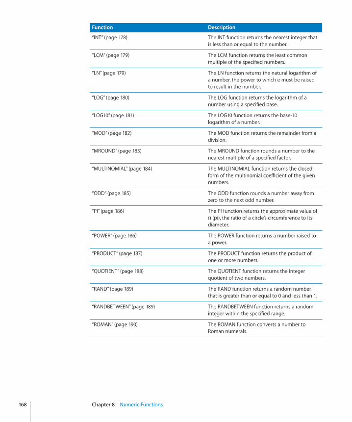
Function Description
“INT” (page 178) The INT function returns the nearest integer that is less than or equal to the number.
“LCM” (page 179) The LCM function returns the least common multiple of the specified numbers.
“LN” (page 179) The LN function returns the natural logarithm of a number, the power to which e must be raised to result in the number.
“LOG” (page 180) The LOG function returns the logarithm of a number using a specified base.
“LOG10” (page 181) The LOG10 function returns the base-10 logarithm of a number.
“MOD” (page 182) The MOD function returns the remainder from a division.
“MROUND” (page 183) The MROUND function rounds a number to the nearest multiple of a specified factor.
“MULTINOMIAL” (page 184) The MULTINOMIAL function returns the closed form of the multinomial coefficient of the given numbers.
“ODD” (page 185) The ODD function rounds a number away from zero to the next odd number.
“PI” (page 186) The PI function returns the approximate value of π (pi), the ratio of a circle’s circumference to its diameter.
“POWER” (page 186) The POWER function returns a number raised to a power.
“PRODUCT” (page 187) The PRODUCT function returns the product of one or more numbers.
“QUOTIENT” (page 188) The QUOTIENT function returns the integer quotient of two numbers.
“RAND” (page 189) The RAND function returns a random number that is greater than or equal to 0 and less than 1.
“RANDBETWEEN” (page 189) The RANDBETWEEN function returns a random integer within the specified range.
“ROMAN” (page 190) The ROMAN function converts a number to Roman numerals.
168 Chapter 8 Numeric Functions

Chapter 8 Numeric Functions 169
Function Description
“ROUND” (page 191) The ROUND function returns a number rounded to the specified number of places.
“ROUNDDOWN” (page 192) The ROUNDDOWN function returns a number rounded toward zero (rounded down) to the specified number of places.
“ROUNDUP” (page 193) The ROUNDUP function returns a number rounded away from zero (rounded up) to the specified number of places.
“SIGN” (page 195) The SIGN function returns 1 when a given number is positive, –1 when it is negative, and 0 when it is zero.
“SQRT” (page 195) The SQRT function returns the square root of a number.
“SQRTPI” (page 196) The SQRTPI function returns the square root of a number multiplied by π (pi).
“SUM” (page 196) The SUM function returns the sum of a collection of numbers.
“SUMIF” (page 197) The SUMIF function returns the sum of a collection of numbers, including only numbers that satisfy a specified condition.
“SUMIFS” (page 198) The SUMIFS function returns the sum of the cells in a collection where the test values meet the given conditions.
“SUMPRODUCT” (page 200) The SUMPRODUCT function returns the sum of the products of corresponding numbers in one or more ranges.
“SUMSQ” (page 201) The SUMSQ function returns the sum of the squares of a collection of numbers.
“SUMX2MY2” (page 202) The SUMX2MY2 function returns the sum of the difference of the squares of corresponding values in two collections.
“SUMX2PY2” (page 203) The SUMX2PY2 function returns the sum of the squares of corresponding values in two collections.
“SUMXMY2” (page 204) The SUMXMY2 function returns the sum of the squares of the differences between corresponding values in two collections.
“TRUNC” (page 204) The TRUNC function truncates a number to the specified number of digits.

ABSThe ABS function returns the absolute value of a number or duration.
ABS(num-dur)
 num-dur:� A number or duration value. num-dur is a number or duration value.
Usage NotesThe result returned by ABS is either a positive number or 0. Â
Examples
=ABS(A1) returns 5, if cell A1 contains 5.
=ABS(8-5) returns 3.
=ABS(5-8) returns 3.
=ABS(0) returns 0.
=ABS(A1) returns 0, if cell A1 is empty.
Related TopicsFor related functions and additional information, see:
“Listing of Numeric Functions” on page 167
“Value Types” on page 36
“The Elements of Formulas” on page 15
“Using the Keyboard and Mouse to Create and Edit Formulas” on page 26
“Pasting from Examples in Help” on page 41
CEILINGThe CEILING function rounds a number away from zero to the nearest multiple of the specified factor.
CEILING(num-to-round, multiple-factor)
 num-to-round:� The number to be rounded. num-to-round is a number value.
 multiple-factor:� The number to use to determine the closet multiple. multiple-factor is a number value and must have the same sign as num-to-round.
170 Chapter 8 Numeric Functions

Chapter 8 Numeric Functions 171
Examples
=CEILING(0.25, 1) returns 1.
=CEILING(1.25, 1) returns 2.
=CEILING(-1.25, -1) returns -2.
=CEILING(5, 2) returns 6.
=CEILING(73, 10) returns 80.
=CEILING(7, 2.5) returns 7.5.
Related TopicsFor related functions and additional information, see:
“EVEN” on page 173
“FLOOR” on page 176
“INT” on page 178
“MROUND” on page 183
“ODD” on page 185
“ROUND” on page 191
“ROUNDDOWN” on page 192
“ROUNDUP” on page 193
“TRUNC” on page 204
“More on Rounding” on page 355
“Listing of Numeric Functions” on page 167
“Value Types” on page 36
“The Elements of Formulas” on page 15
“Using the Keyboard and Mouse to Create and Edit Formulas” on page 26
“Pasting from Examples in Help” on page 41

COMBINThe COMBIN function returns the number of different ways you can combine a number of items into groups of a specific size, ignoring the order within the groups.
COMBIN(total-items, group-size)
 total-items:� The total number of items. total-items is a number value and must be greater than or equal to 0. If total-items has a decimal (fractional) part, it is ignored.
 group-size:� The number of items combined in each group. group-size is a number value and must be greater than or equal to 0. If group-size has a decimal (fractional) part, it is ignored.
Usage NotesCombinations are not the same as permutations. The order of the items in a group is Âignored for combinations but not for permutations. For example, (1, 2, 3) and (3, 2, 1) are the same combination but two unique permutations. If you want the number of permutations rather than the number of combinations, use the PERMUT function.
Examples
=COMBIN(3, 2) returns 3, the number of unique groups you can create if you start with 3 items and group them 2 at a time.
=COMBIN(3.2, 2.3) returns 3. Fractional parts are dropped.
=COMBIN(5, 2) and =COMBIN(5, 3) both return 10.
Related TopicsFor related functions and additional information, see:
“PERMUT” on page 281
“Listing of Numeric Functions” on page 167
“Value Types” on page 36
“The Elements of Formulas” on page 15
“Using the Keyboard and Mouse to Create and Edit Formulas” on page 26
“Pasting from Examples in Help” on page 41
172 Chapter 8 Numeric Functions

Chapter 8 Numeric Functions 173
EVENThe EVEN function rounds a number away from zero to the next even number.
EVEN(num-to-round)
 num-to-round:� The number to be rounded. num-to-round is a number value.
Usage NotesTo round to an odd number, use the ODD function. Â
Examples
=EVEN(1) returns 2.
=EVEN(2) returns 2.
=EVEN(2.5) returns 4.
=EVEN(-2.5) returns -4.
=EVEN(0) returns 0.
Related TopicsFor related functions and additional information, see:
“CEILING” on page 170
“FLOOR” on page 176
“INT” on page 178
“MROUND” on page 183
“ODD” on page 185
“ROUND” on page 191
“ROUNDDOWN” on page 192
“ROUNDUP” on page 193
“TRUNC” on page 204
“More on Rounding” on page 355
“Listing of Numeric Functions” on page 167
“Value Types” on page 36
“The Elements of Formulas” on page 15
“Using the Keyboard and Mouse to Create and Edit Formulas” on page 26
“Pasting from Examples in Help” on page 41

EXPThe EXP function returns e (the base of natural logarithms) raised to the specified power.
EXP(exponent)
 exponent:� The power to which you want to raise e. exponent is a number value.
Usage NotesEXP and LN are mathematically inverses over the domain where LN is defined, but Âbecause of floating-point rounding, EXP(LN(x)) may not give exactly x.
Example
=EXP(1) returns 2.71828182845905, an approximation of e.
Related TopicsFor related functions and additional information, see:
“LN” on page 179
“Listing of Numeric Functions” on page 167
“Value Types” on page 36
“The Elements of Formulas” on page 15
“Using the Keyboard and Mouse to Create and Edit Formulas” on page 26
“Pasting from Examples in Help” on page 41
FACTThe FACT function returns the factorial of a number.
FACT(fact-num)
 fact-num:� A number. fact-num is a number value and must be greater than or equal to 0. Any decimal (fractional) part of fact-num is ignored.
Examples
=FACT(5) returns 120, or 1 * 2 * 3 * 4 * 5.
=FACT(0) returns 1.
=FACT(4.5) returns 24. The fraction is dropped and 4 factorial is computed.
=FACT(-1) returns an error; the number must be nonnegative.
174 Chapter 8 Numeric Functions
Chapter 8 Numeric Functions 175
Related TopicsFor related functions and additional information, see:
“FACTDOUBLE” on page 175
“MULTINOMIAL” on page 184
“Listing of Numeric Functions” on page 167
“Value Types” on page 36
“The Elements of Formulas” on page 15
“Using the Keyboard and Mouse to Create and Edit Formulas” on page 26
“Pasting from Examples in Help” on page 41
FACTDOUBLEThe FACTDOUBLE function returns the double factorial of a number.
FACTDOUBLE(fact-num)
 fact-num:� A number. fact-num is a number value and must be greater than or equal to –1. Values in the range –1 to 1 return 1. Any decimal (fractional) part of fact-num is ignored.
Usage NotesFor an even integer, the double factorial is the product of all even integers less than Âor equal to the given integer and greater than or equal to 2. For an odd integer, the double factorial is the product of all odd integers less than or equal to the given integer and greater than or equal to 1.
Examples
=FACTDOUBLE(4) returns 8, the product of 2 and 4.
=FACTDOUBLE(4.7) returns 8, the product of 2 and 4. The decimal portion is ignored.
=FACTDOUBLE (10) returns 3840, the product of 2, 4, 6, 8, and 10.
=FACTDOUBLE(1) returns 1, as all numbers between –1 and 1 return 1.
=FACTDOUBLE(-1) returns 1, as all numbers between –1 and 1 return 1.
=FACTDOUBLE (7) returns 105, the product of 1, 3, 5, and 7.
Related TopicsFor related functions and additional information, see:
“FACT” on page 174
“MULTINOMIAL” on page 184

“Listing of Numeric Functions” on page 167
“Value Types” on page 36
“The Elements of Formulas” on page 15
“Using the Keyboard and Mouse to Create and Edit Formulas” on page 26
“Pasting from Examples in Help” on page 41
FLOORThe FLOOR function rounds a number toward zero to the nearest multiple of the specified factor.
FLOOR(num-to-round, factor)
 num-to-round:� The number to be rounded. num-to-round is a number value.
 factor:� The number to use to determine the closet multiple. factor is a number value. It must have the same sign as num-to-round.
Examples
=FLOOR(0.25, 1) returns 0.
=FLOOR(1.25, 1) returns 1.
=FLOOR(5, 2) returns 4.
=FLOOR(73, 10) returns 70.
=FLOOR(-0.25, -1) returns 0.
=FLOOR(9, 2.5) returns 7.5.
Related TopicsFor related functions and additional information, see:
“CEILING” on page 170
“EVEN” on page 173
“INT” on page 178
“MROUND” on page 183
“ODD” on page 185
“ROUND” on page 191
“ROUNDDOWN” on page 192
“ROUNDUP” on page 193
176 Chapter 8 Numeric Functions

Chapter 8 Numeric Functions 177
“TRUNC” on page 204
“More on Rounding” on page 355
“Listing of Numeric Functions” on page 167
“Value Types” on page 36
“The Elements of Formulas” on page 15
“Using the Keyboard and Mouse to Create and Edit Formulas” on page 26
“Pasting from Examples in Help” on page 41
GCDThe GCD function returns the greatest common divisor of the specified numbers.
GCD(num-value, num-value…)
 num-value:� A number. num-value is a number value. If there is a decimal portion it is ignored.
 num-value…: Optionally include one or more additional numbers.
Usage NotesSometimes called the greatest common factor, the greatest common divisor is the Âlargest integer that divides into each of the numbers with no remainder.
Examples
=GCD(8, 10) returns 2.
=GCD(99, 102, 105) returns 3.
=GCD(34, 51) returns 17.
Related TopicsFor related functions and additional information, see:
“LCM” on page 179
“Listing of Numeric Functions” on page 167
“Value Types” on page 36
“The Elements of Formulas” on page 15
“Using the Keyboard and Mouse to Create and Edit Formulas” on page 26
“Pasting from Examples in Help” on page 41

INTThe INT function returns the nearest integer that is less than or equal to the number.
INT(num-to-round)
 num-to-round:� The number to be rounded. num-to-round is a number value.
Examples
=INT(1.49) returns 1.
=INT(1.50) returns 1.
=INT(1.23456) returns 1.
=INT(1111.222) returns 1111.
=INT(-2.2) returns -3.
=INT(-2.8) returns -3.
Related TopicsFor related functions and additional information, see:
“CEILING” on page 170
“EVEN” on page 173
“FLOOR” on page 176
“MROUND” on page 183
“ODD” on page 185
“ROUND” on page 191
“ROUNDDOWN” on page 192
“ROUNDUP” on page 193
“TRUNC” on page 204
“More on Rounding” on page 355
“Listing of Numeric Functions” on page 167
“Value Types” on page 36
“The Elements of Formulas” on page 15
“Using the Keyboard and Mouse to Create and Edit Formulas” on page 26
“Pasting from Examples in Help” on page 41
178 Chapter 8 Numeric Functions

Chapter 8 Numeric Functions 179
LCMThe LCM function returns the least common multiple of the specified numbers.
LCM(num-value, num-value…)
 num-value:� A number. num-value is a number value.
 num-value…: Optionally include one or more additional numbers.
Usage NotesSometimes called the lowest or smallest common multiple, the least common Âmultiple is the smallest integer that is a multiple of the specified numbers.
Examples
=LCM(2, 3) returns 6.
=LCM(34, 68) returns 68.
=LCM(30, 40, 60) returns 120.
=LCM(30.25, 40.333, 60.5) returns 120 (the fractional parts are ignored).
=LCM(2, -3) displays an error (negative numbers are not allowed).
Related TopicsFor related functions and additional information, see:
“GCD” on page 177
“Listing of Numeric Functions” on page 167
“Value Types” on page 36
“The Elements of Formulas” on page 15
“Using the Keyboard and Mouse to Create and Edit Formulas” on page 26
“Pasting from Examples in Help” on page 41
LNThe LN function returns the natural logarithm of a number, the power to which e must be raised to result in the number.
LN(pos-num)
 pos-num:� A positive number. pos-num is a number value and must be greater than 0.
Usage NotesEXP and LN are mathematically inverses over the domain where LN is defined, but Âbecause of floating-point rounding, =LN(EXP(x)) may not give exactly x.

Example
=LN(2.71828) returns approximately 1, the power to which e must be raised to produce 2.71828.
Related TopicsFor related functions and additional information, see:
“EXP” on page 174
“LOG” on page 180
“LOGINV” on page 268
“LOGNORMDIST” on page 269
“Listing of Numeric Functions” on page 167
“Value Types” on page 36
“The Elements of Formulas” on page 15
“Using the Keyboard and Mouse to Create and Edit Formulas” on page 26
“Pasting from Examples in Help” on page 41
LOGThe LOG function returns the logarithm of a number using a specified base.
LOG(pos-num, base)
 pos-num:� A positive number. pos-num is a number value and must be greater than 0.
 base:� An optional value specifying the base of the logarithm. base is a number value and must be greater than 0. If base is 1, a division by zero will result and the function will return an error. If base is omitted, it is assumed to be 10.
Examples
=LOG(8, 2) returns 3.
=LOG(100, 10) and LOG(100) both return 2.
=LOG(5.0625, 1.5) returns 4.
Related TopicsFor related functions and additional information, see:
“LOG10” on page 181
“Listing of Numeric Functions” on page 167
180 Chapter 8 Numeric Functions

Chapter 8 Numeric Functions 181
“Value Types” on page 36
“The Elements of Formulas” on page 15
“Using the Keyboard and Mouse to Create and Edit Formulas” on page 26
“Pasting from Examples in Help” on page 41
LOG10The LOG10 function returns the base-10 logarithm of a number.
LOG10(pos-num)
 pos-num:� A positive number. pos-num is a number value and must be greater than 0.
Usage NotesTo find the logarithm for a base other than 10, use the LOG function. Â
Examples
=LOG10(1) returns 0.
=LOG10(10) returns 1.
=LOG10(100) returns 2.
=LOG10(1000) returns 3.
Related TopicsFor related functions and additional information, see:
“LN” on page 179
“LOG” on page 180
“Listing of Numeric Functions” on page 167
“Value Types” on page 36
“The Elements of Formulas” on page 15
“Using the Keyboard and Mouse to Create and Edit Formulas” on page 26
“Pasting from Examples in Help” on page 41

MODThe MOD function returns the remainder from a division.
MOD(dividend, divisor)
 dividend:� A number to be divided by another number. dividend is a number value.
 divisor:� A number to divide into another number. divisor is a number value. If 0, a division by zero will result and the function will return an error.
Usage NotesThe sign of the result matches that of the divisor. Â
When computing MOD(a, b), MOD gives a number r such that a = bk + r, where r is Âbetween 0 and b, and k is an integer.
MOD(a, b) is equivalent to a–b*INT(a/b). Â
Examples
=MOD(6, 3) returns 0.
=MOD(7, 3) returns 1.
=MOD(8, 3) returns 2.
=MOD(-8, 3) returns 1.
=MOD(4.5, 2) returns 0.5.
=MOD(7, 0.75) returns 0.25.
Related TopicsFor related functions and additional information, see:
“QUOTIENT” on page 188
“Listing of Numeric Functions” on page 167
“Value Types” on page 36
“The Elements of Formulas” on page 15
“Using the Keyboard and Mouse to Create and Edit Formulas” on page 26
“Pasting from Examples in Help” on page 41
182 Chapter 8 Numeric Functions

Chapter 8 Numeric Functions 183
MROUNDThe MROUND function rounds a number to the nearest multiple of a specified factor.
MROUND(num-to-round, factor)
 num-to-round:� The number to be rounded. num-to-round is a number value.
 factor:� The number to use to determine the closet multiple. factor is a number value. It must have the same sign as num-to-round.
Examples
=MROUND(2, 3) returns 3.
=MROUND(4, 3) returns 3.
=MROUND(4.4999, 3) returns 3.
=MROUND(4.5, 3) returns 6.
=MROUND(-4.5, 3) returns an error.
Related TopicsFor related functions and additional information, see:
“CEILING” on page 170
“EVEN” on page 173
“FLOOR” on page 176
“INT” on page 178
“ODD” on page 185
“ROUND” on page 191
“ROUNDDOWN” on page 192
“ROUNDUP” on page 193
“TRUNC” on page 204
“More on Rounding” on page 355
“Listing of Numeric Functions” on page 167
“Value Types” on page 36
“The Elements of Formulas” on page 15
“Using the Keyboard and Mouse to Create and Edit Formulas” on page 26
“Pasting from Examples in Help” on page 41

MULTINOMIALThe MULTINOMIAL function returns the multinomial coefficient of the given numbers. It accomplishes this by determining the ratio of the factorial of the sum of the given numbers to the product of the factorials of the given numbers.
MULTINOMIAL(non-neg-num, non-neg-num…)
 non-neg-num:� A number. non-neg-num is a number value and must be greater than or equal to 0.
 non-neg-num…: Optionally include one or more additional numbers.
Examples
=MULTINOMIAL(2) returns 1. The factorial of the 2 is 2. The product of 1 and 2 is 2. The ratio of 2:2 is 1.
=MULTINOMIAL(1, 2, 3) returns 60. The factorial of the sum of 1, 2, and 3 is 720. The product of the factorials of 1, 2, and 3 is 12. The ratio of 720:12 is 60.
=MULTINOMIAL(4, 5, 6) returns 630630. The factorial of the sum of 4, 5, and 6 is 1.30767E+12. The product of the factorials of 4, 5, and 6 is 2073600. The ratio of 1.30767E+12:2073600 is 630630.
Related TopicsFor related functions and additional information, see:
“FACT” on page 174
“FACTDOUBLE” on page 175
“Listing of Numeric Functions” on page 167
“Value Types” on page 36
“The Elements of Formulas” on page 15
“Using the Keyboard and Mouse to Create and Edit Formulas” on page 26
“Pasting from Examples in Help” on page 41
184 Chapter 8 Numeric Functions

Chapter 8 Numeric Functions 185
ODDThe ODD function rounds a number away from zero to the next odd number.
ODD(num-to-round)
 num-to-round:� The number to be rounded. num-to-round is a number value.
Usage NotesTo round to an even number, use the EVEN function. Â
Examples
=ODD(1) returns 1.
=ODD(2) returns 3.
=ODD(2.5) returns 3.
=ODD(-2.5) returns -3.
=ODD(0) returns 1.
Related TopicsFor related functions and additional information, see:
“CEILING” on page 170
“EVEN” on page 173
“FLOOR” on page 176
“INT” on page 178
“MROUND” on page 183
“ROUND” on page 191
“ROUNDDOWN” on page 192
“ROUNDUP” on page 193
“TRUNC” on page 204
“More on Rounding” on page 355
“Listing of Numeric Functions” on page 167
“Value Types” on page 36
“The Elements of Formulas” on page 15
“Using the Keyboard and Mouse to Create and Edit Formulas” on page 26
“Pasting from Examples in Help” on page 41

PIThe PI function returns the approximate value of π (pi), the ratio of a circle’s circumference to its diameter.
PI()
Usage NotesThe PI function does not have any arguments. However, you must include the Âparentheses: =PI().
PI is accurate to 15 decimal places. Â
Examples
=PI() returns 3.14159265358979.
=SIN(PI()/2) returns 1, the sine of π/2 radians or 90 degrees.
Related TopicsFor related functions and additional information, see:
“COS” on page 333
“SIN” on page 336
“TAN” on page 338
“Listing of Numeric Functions” on page 167
“Value Types” on page 36
“The Elements of Formulas” on page 15
“Using the Keyboard and Mouse to Create and Edit Formulas” on page 26
“Pasting from Examples in Help” on page 41
POWERThe POWER function returns a number raised to a power.
POWER(number, exponent)
 number:� A number. number is a number value.
 exponent:� The power to which to raise the given number. exponent is a number value.
Usage NotesThe POWER function produces the same result as the ^ operator: =POWER(x, y) Âreturns the same result as =x^y.
186 Chapter 8 Numeric Functions

Chapter 8 Numeric Functions 187
Examples
=POWER(2, 3) returns 8.
=POWER(2, 10) returns 1024.
=POWER(0.5, 3) returns 0.125.
=POWER(100, 0.5) returns 10.
Related TopicsFor related functions and additional information, see:
“Listing of Numeric Functions” on page 167
“Value Types” on page 36
“The Elements of Formulas” on page 15
“Using the Keyboard and Mouse to Create and Edit Formulas” on page 26
“Pasting from Examples in Help” on page 41
PRODUCTThe PRODUCT function returns the product of one or more numbers.
PRODUCT(num-value, num-value…)
 num-value:� A number. num-value is a number value.
 num-value…: Optionally include one or more additional numbers.
Usage NotesEmpty cells included within the values are ignored and do not affect the result. Â
Examples
=PRODUCT(2, 4) returns 8.
=PRODUCT(0.5, 5, 4, 5) returns 50.
Related TopicsFor related functions and additional information, see:
“SUM” on page 196
“Listing of Numeric Functions” on page 167
“Value Types” on page 36
“The Elements of Formulas” on page 15

“Using the Keyboard and Mouse to Create and Edit Formulas” on page 26
“Pasting from Examples in Help” on page 41
QUOTIENTThe QUOTIENT function returns the integer quotient of two numbers.
QUOTIENT(dividend, divisor)
 dividend:� A number to be divided by another number. dividend is a number value.
 divisor:� A number to divide into another number. divisor is a number value. If 0, a division by zero will result and the function will return an error.
Usage NotesIf either, but not both, the dividend or divisor is negative, the result will be negative. ÂIf the sign of both the dividend and the divisor is the same, the result will be positive.
Only the whole part of the quotient is returned. The fractional part (or remainder) Âis ignored.
Examples
=QUOTIENT(5, 2) returns 2.
=QUOTIENT(5.99, 2) returns 2.
=QUOTIENT(-5, 2) returns -2.
=QUOTIENT(6, 2) returns 3.
=QUOTIENT(5, 6) returns 0.
Related TopicsFor related functions and additional information, see:
“MOD” on page 182
“Listing of Numeric Functions” on page 167
“Value Types” on page 36
“The Elements of Formulas” on page 15
“Using the Keyboard and Mouse to Create and Edit Formulas” on page 26
“Pasting from Examples in Help” on page 41
188 Chapter 8 Numeric Functions

Chapter 8 Numeric Functions 189
RANDThe RAND function returns a random number that is greater than or equal to 0 and less than 1.
RAND()
Usage NotesThe RAND function does not have any arguments. However, you must include the Âparentheses: =RAND().
Any time you change a value in the table, a new random number greater than or Âequal to 0 and less than 1 is generated.
Example
=RAND() returns, for example, 0.217538648284972, 0.6137690856, 0.0296026556752622, and 0.4684193600 for four recalculations.
Related TopicsFor related functions and additional information, see:
“RANDBETWEEN” on page 189
“Listing of Numeric Functions” on page 167
“Value Types” on page 36
“The Elements of Formulas” on page 15
“Using the Keyboard and Mouse to Create and Edit Formulas” on page 26
“Pasting from Examples in Help” on page 41
RANDBETWEENThe RANDBETWEEN function returns a random integer within the specified range.
RANDBETWEEN(lower, upper)
 lower:� The lower limit or bound. lower is a number value.
 upper:� The upper limit or bound. upper is a number value.
Usage NotesAny time you change a value in the table, a new random number between the Âlower and upper limits is generated.
Example
=RANDBETWEEN(1, 10) returns, for example, 8, 6, 2, 3, and 5 for five recalculations.

Related TopicsFor related functions and additional information, see:
“RAND” on page 189
“Listing of Numeric Functions” on page 167
“Value Types” on page 36
“The Elements of Formulas” on page 15
“Using the Keyboard and Mouse to Create and Edit Formulas” on page 26
“Pasting from Examples in Help” on page 41
ROMANThe ROMAN function converts a number to Roman numerals.
ROMAN(arabic-num, roman-style)
 arabic-num:� The Arabic numeral that you want to convert. arabic-num is a number value in the range 0 to 3999.
 roman-style:� An optional value that determines how strictly the classical rules for forming Roman numerals are applied.
strict (0 or TRUE, or omitted):� Use the most strict classical rules. When a smaller numeral precedes a larger to indicate subtraction, the smaller must be a power of 10 and can precede a number no more than 10 times its size. For example, 999 is represented as CMXCIX, but not LMVLIV.
relax by one degree (1):� Relax the strict classical rule by one degree. When a smaller number precedes a larger, the smaller need not be a power of 10 and the relative size rule is extended by one numeral. For example, 999 can be represented as LMVLIV, but not XMIX.
relax by two degrees (2):� Relax the classical rule by two degrees. When a smaller number precedes a larger, the relative size rule is extended by two numerals. For example, 999 can be represented as XMIX, but not VMIV.
relax by three degrees (3):� Relax the classical rule by three degrees. When a smaller number precedes a larger, the relative size rule is extended by three numerals. For example, 999 can be represented as VMIV, but not IM.
relax by four degrees (4 or FALSE):� Relax the classical rule by four degrees. When a smaller number precedes a larger, the relative size rule is extended by four numerals. For example, 999 can be represented as IM.
190 Chapter 8 Numeric Functions

Chapter 8 Numeric Functions 191
Examples
=ROMAN(12) returns XII.
=ROMAN(999) returns CMXCIX.
=ROMAN(999, 1) returns LMVLIV.
=ROMAN(999, 2) returns XMIX.
=ROMAN(999, 3) returns VMIV.
Related TopicsFor related functions and additional information, see:
“Listing of Numeric Functions” on page 167
“Value Types” on page 36
“The Elements of Formulas” on page 15
“Using the Keyboard and Mouse to Create and Edit Formulas” on page 26
“Pasting from Examples in Help” on page 41
ROUNDThe ROUND function returns a number rounded to the specified number of places.
ROUND(num-to-round, digits)
 num-to-round:� The number to be rounded. num-to-round is a number value.
 digits:� The number of digits you want to retain, relative to the decimal point. digits is a number value. A positive number represents digits (decimal places) to the right of the decimal point to include. A negative number specifies digits to the left of the decimal point to replace with zeros (the number of zeros at the end of the number).
Examples
=ROUND(1.49, 0) returns 1.
=ROUND(1.50, 0) returns 2.
=ROUND(1.23456, 3) returns 1.235.
=ROUND(1111.222, -2) returns 1100.
=ROUND(-2.2, 0) returns -2.
=ROUND(-2.8, 0) returns -3.
Related TopicsFor related functions and additional information, see:
“CEILING” on page 170

“EVEN” on page 173
“FLOOR” on page 176
“INT” on page 178
“MROUND” on page 183
“ODD” on page 185
“ROUNDDOWN” on page 192
“ROUNDUP” on page 193
“TRUNC” on page 204
“More on Rounding” on page 355
“Listing of Numeric Functions” on page 167
“Value Types” on page 36
“The Elements of Formulas” on page 15
“Using the Keyboard and Mouse to Create and Edit Formulas” on page 26
“Pasting from Examples in Help” on page 41
ROUNDDOWNThe ROUNDDOWN function returns a number rounded toward zero (rounded down) to the specified number of places.
ROUNDDOWN(num-to-round, digits)
 num-to-round:� The number to be rounded. num-to-round is a number value.
 digits:� The number of digits you want to retain, relative to the decimal point. digits is a number value. A positive number represents digits (decimal places) to the right of the decimal point to include. A negative number specifies digits to the left of the decimal point to replace with zeros (the number of zeros at the end of the number).
Examples
=ROUNDDOWN(1.49, 0) returns 1.
=ROUNDDOWN(1.50, 0) returns 1.
=ROUNDDOWN(1.23456, 3) returns 1.234.
=ROUNDDOWN(1111.222, -2) returns 1100.
=ROUNDDOWN(-2.2, 0) returns -2.
=ROUNDDOWN(-2.8, 0) returns -2.
192 Chapter 8 Numeric Functions

Chapter 8 Numeric Functions 193
Related TopicsFor related functions and additional information, see:
“CEILING” on page 170
“EVEN” on page 173
“FLOOR” on page 176
“INT” on page 178
“MROUND” on page 183
“ODD” on page 185
“ROUND” on page 191
“ROUNDUP” on page 193
“TRUNC” on page 204
“More on Rounding” on page 355
“Listing of Numeric Functions” on page 167
“Value Types” on page 36
“The Elements of Formulas” on page 15
“Using the Keyboard and Mouse to Create and Edit Formulas” on page 26
“Pasting from Examples in Help” on page 41
ROUNDUPThe ROUNDUP function returns a number rounded away from zero (rounded up) to the specified number of places.
ROUNDUP(num-to-round, digits)
 num-to-round:� The number to be rounded. num-to-round is a number value.
 digits:� The number of digits you want to retain, relative to the decimal point. digits is a number value. A positive number represents digits (decimal places) to the right of the decimal point to include. A negative number specifies digits to the left of the decimal point to replace with zeros (the number of zeros at the end of the number).

Examples
=ROUNDUP(1.49, 0) returns 2.
=ROUNDUP(1.50, 0) returns 2.
=ROUNDUP(1.23456, 3) returns 1.235.
=ROUNDUP(1111.222, -2) returns 1200.
=ROUNDUP(-2.2, 0) returns -3.
=ROUNDUP(-2.8, 0) returns -3.
Related TopicsFor related functions and additional information, see:
“CEILING” on page 170
“EVEN” on page 173
“FLOOR” on page 176
“INT” on page 178
“MROUND” on page 183
“ODD” on page 185
“ROUND” on page 191
“ROUNDDOWN” on page 192
“TRUNC” on page 204
“More on Rounding” on page 355
“Listing of Numeric Functions” on page 167
“Value Types” on page 36
“The Elements of Formulas” on page 15
“Using the Keyboard and Mouse to Create and Edit Formulas” on page 26
“Pasting from Examples in Help” on page 41
194 Chapter 8 Numeric Functions

Chapter 8 Numeric Functions 195
SIGNThe SIGN function returns 1 when the argument number is positive, –1 when it is negative, and 0 when it is zero.
SIGN(num)
 num:� A number. number is a number value.
Examples
=SIGN(2) returns 1.
=SIGN(0) returns 0.
=SIGN(-2) returns -1.
=SIGN(A4) returns -1, if cell A4 contains -2.
Related TopicsFor related functions and additional information, see:
“Listing of Numeric Functions” on page 167
“Value Types” on page 36
“The Elements of Formulas” on page 15
“Using the Keyboard and Mouse to Create and Edit Formulas” on page 26
“Pasting from Examples in Help” on page 41
SQRTThe SQRT function returns the square root of a number.
SQRT(num)
 num:� A number. number is a number value.
Examples
=SQRT(16) returns 4.
=SQRT(12.25) returns 3.5, the square root of 12.25.
Related TopicsFor related functions and additional information, see:
“Listing of Numeric Functions” on page 167
“Value Types” on page 36
“The Elements of Formulas” on page 15

“Using the Keyboard and Mouse to Create and Edit Formulas” on page 26
“Pasting from Examples in Help” on page 41
SQRTPIThe SQRTPI function returns the square root of a number after it has been multiplied by π (pi).
SQRTPI(non-neg-number)
 non-neg-number:� A nonnegative number. non-neg-num is a number value and must be greater than or equal to 0.
Examples
=SQRTPI(5) returns 3.96332729760601.
=SQRTPI(8) returns 5.013256549262.
Related TopicsFor related functions and additional information, see:
“Listing of Numeric Functions” on page 167
“Value Types” on page 36
“The Elements of Formulas” on page 15
“Using the Keyboard and Mouse to Create and Edit Formulas” on page 26
“Pasting from Examples in Help” on page 41
SUMThe SUM function returns the sum of a collection of numbers.
SUM(num-date-dur, num-date-dur…)
 num-date-dur:� A value. num-date-dur is a number value, a date/time value, or a duration value.
 num-date-dur…: Optionally include one or more additional values. If more than one num-date-dur value is specified, they must all be of the same type.
Usage NotesThere is one case where all values do not have to be of the same type. If exactly one Âdate/time value is included, any number values are considered to be numbers of days and all numbers and duration values are added to the date/time value.
196 Chapter 8 Numeric Functions

Chapter 8 Numeric Functions 197
Date/time values can’t be added together, so only one date/time value (as discussed Âabove) is permitted.
The values can be in individual cells, ranges of cells, or included directly as Âarguments to the function.
Examples
=SUM(A1:A4) adds the numbers in four cells.
=SUM(A1:D4) adds the numbers in a square array of sixteen cells.
=SUM(A1:A4, 100) adds the numbers in four cells plus 100.
Related TopicsFor related functions and additional information, see:
“PRODUCT” on page 187
“Listing of Numeric Functions” on page 167
“Value Types” on page 36
“The Elements of Formulas” on page 15
“Using the Keyboard and Mouse to Create and Edit Formulas” on page 26
“Pasting from Examples in Help” on page 41
SUMIFThe SUMIF function returns the sum of a collection of numbers, including only numbers that satisfy a specified condition.
SUMIF(test-values, condition, sum-values)
 test-values:� The collection containing the values to be tested. test-values is a collection containing any value type.
 condition:� An expression that results in a logical TRUE or FALSE. condition is an expression that can contain anything as long as the result from comparing condition to a value in test-values can be expressed as a Boolean value of TRUE or FALSE.
 sum-values:� An optional collection containing the numbers to be summed. sum-values is a collection containing number, date/time, or duration values. It should have the same dimensions as test-values.
Usage NotesIf  sum-values is omitted, the default value is test-values.
Although  test-values can contain any type of value, it should usually contain values all of the same type.

If  sum-values is omitted, test-values would normally contain only number or duration values.
Examples
Given the following table:
=SUMIF(A1:A8, “<5”) returns 10.
=SUMIF(A1:A8, “<5”, B1:B8) returns 100.
=SUMIF(D1:F3, “=c”, D5:F7) returns 27.
=SUMIF(B1:D1, 1) or SUMIF(B1:D1, SUM(1)) both total all the occurrences of 1 in the range.
Related TopicsFor related functions and additional information, see:
“AVERAGEIF” on page 233
“AVERAGEIFS” on page 234
“COUNTIF” on page 247
“COUNTIFS” on page 248
“SUMIFS” on page 198
“Specifying Conditions and Using Wildcards” on page 360
“Listing of Numeric Functions” on page 167
“Value Types” on page 36
“The Elements of Formulas” on page 15
“Using the Keyboard and Mouse to Create and Edit Formulas” on page 26
“Pasting from Examples in Help” on page 41
SUMIFSThe SUMIFS function returns the sum of the cells in a collection where the test values meet the given conditions.
198 Chapter 8 Numeric Functions

Chapter 8 Numeric Functions 199
SUMIFS(sum-values, test-values, condition, test-values…, condition…)
 sum-values:� A collection containing the values to be summed. sum-values is a collection containing number, date/time, or duration values.
 test-values:� A collection containing values to be tested. test-values is a collection containing any type of value.
 condition:� An expression that results in a logical TRUE or FALSE. condition is an expression that can contain anything as long as the result from comparing condition to a value in test-values can be expressed as a Boolean value of TRUE or FALSE.
 test-values…: Optionally include one or more additional collections containing values to be tested. Each test-values collection must be followed immediately with a condition expression. This pattern of test-values, condition can be repeated as many times as needed.
 condition…: If an optional collection of test-values is included, an expression that results in a logical TRUE or FALSE. There must be one condition following each test-values collection; therefore, this function will always have an odd number of arguments.
Usage NotesFor each of the test and condition value pairs, the corresponding (same position Âwithin range or array) cell or value is compared to the condition. If all of the conditions are met, the corresponding cell or value in sum-values is included in the sum.
All arrays must be of the same size. Â
Examples
The following table shows part of a ledger of deliveries of a certain commodity. Each load is weighed, rated either 1 or 2, and the date of the delivery is noted.
=SUMIFS(A2:A13,B2:B13,”=1”,C2:C13,”>=12/13/2010”,C2:C13,”<=12/17/2010”) returns 23, the number of tons of the commodity delivered during the week of December 17 that were rated “1.”
=SUMIFS(A2:A13,B2:B13,”=2”,C2:C13,”>=12/13/2010”,C2:C13,”<=12/17/2010”) returns 34, the number of tons of the commodity delivered during the same week that were rated “2.”

Related TopicsFor related functions and additional information, see:
“AVERAGEIF” on page 233
“AVERAGEIFS” on page 234
“COUNTIF” on page 247
“COUNTIFS” on page 248
“SUMIF” on page 197
“Specifying Conditions and Using Wildcards” on page 360
“Listing of Numeric Functions” on page 167
“Value Types” on page 36
“The Elements of Formulas” on page 15
“Using the Keyboard and Mouse to Create and Edit Formulas” on page 26
“Pasting from Examples in Help” on page 41
SUMPRODUCTThe SUMPRODUCT function returns the sum of the products of corresponding numbers in one or more ranges.
SUMPRODUCT(range, range…)
 range:� A range of cells. range is a reference to a single range of cells containing values of any type. If string or Boolean values are included in range, they are ignored.
 range…: Optionally include one or more additional ranges of cells. The ranges must all have the same dimensions.
Usage NotesThe SUMPRODUCT function multiplies the corresponding numbers in each range Âand then sums each of the products. If only one range is specified, SUMPRODUCT returns the sum of the range.
Examples
=SUMPRODUCT(3, 4) returns 12.
=SUMPRODUCT({1, 2}, {3, 4}) = 3 + 8 = 11.
200 Chapter 8 Numeric Functions
Chapter 8 Numeric Functions 201
Related TopicsFor related functions and additional information, see:
“Listing of Numeric Functions” on page 167
“Value Types” on page 36
“The Elements of Formulas” on page 15
“Using the Keyboard and Mouse to Create and Edit Formulas” on page 26
“Pasting from Examples in Help” on page 41
SUMSQThe SUMSQ function returns the sum of the squares of a collection of numbers.
SUMSQ(num-value, num-value…)
 num-value:� A number. num-value is a number value.
 num-value…: Optionally include one or more additional numbers.
Usage NotesThe numbers can be in individual cells, or ranges of cells, or be included directly as Âarguments to the function.
Examples
=SUMSQ(3, 4) returns 25.
=SUMSQ(A1:A4) adds the squares of the list of four numbers.
=SUMSQ(A1:D4) adds the squares of the 16 numbers in a square array of cells.
=SUMSQ(A1:A4, 100) adds the squares of the numbers in four cells plus 100.
=SQRT(SUMSQ(3, 4)) returns 5, using the Pythagorean theorem to find the length of the hypotenuse of a triangle with sides 3 and 4.
Related TopicsFor related functions and additional information, see:
“Listing of Numeric Functions” on page 167
“Value Types” on page 36
“The Elements of Formulas” on page 15
“Using the Keyboard and Mouse to Create and Edit Formulas” on page 26
“Pasting from Examples in Help” on page 41

SUMX2MY2The SUMX2MY2 function returns the sum of the difference of the squares of corresponding values in two collections.
SUMX2MY2(set-1-values, set-2-values)
 set-1-values:� The first collection of values. set-1-values is a collection containing number values.
 set-2-values:� The second collection of values. set-2-values is a collection containing number values.
Example
Given the following table:
=SUMX2MY2(A1:A6,B1:B6) returns –158, the sum of the differences of the squares of the values in column A and the squares of the values in column B. The formula for the first such difference is A12 – B12.
Related TopicsFor related functions and additional information, see:
“Listing of Numeric Functions” on page 167
“Value Types” on page 36
“The Elements of Formulas” on page 15
“Using the Keyboard and Mouse to Create and Edit Formulas” on page 26
“Pasting from Examples in Help” on page 41
202 Chapter 8 Numeric Functions

Chapter 8 Numeric Functions 203
SUMX2PY2The SUMX2PY2 function returns the sum of the squares of corresponding values in two collections.
SUMX2PY2(set-1-values, set-2-values)
 set-1-values:� The first collection of values. set-1-values is a collection containing number values.
 set-2-values:� The second collection of values. set-2-values is a collection containing number values.
Example
Given the following table:
=SUMX2PY2(A1:A6,B1:B6) returns 640, the sum of the squares of the values in column A and the squares of the values in column B. The formula for the first such sum is A12+ B12.
Related TopicsFor related functions and additional information, see:
“Listing of Numeric Functions” on page 167
“Value Types” on page 36
“The Elements of Formulas” on page 15
“Using the Keyboard and Mouse to Create and Edit Formulas” on page 26
“Pasting from Examples in Help” on page 41

SUMXMY2The SUMXMY2 function returns the sum of the squares of the differences between corresponding values in two collections.
SUMXMY2(set-1-values, set-2-values)
 set-1-values:� The first collection of values. set-1-values is a collection containing number values.
 set-2-values:� The second collection of values. set-2-values is a collection containing number values.
Example
Given the following table:
=SUMXMY2(A1:A6,B1:B6) returns 196, the sum of the squares of the values in column A and the squares of the values in column B. The formula for the first such sum is (A1 – B1)2.
Related TopicsFor related functions and additional information, see:
“Listing of Numeric Functions” on page 167
“Value Types” on page 36
“The Elements of Formulas” on page 15
“Using the Keyboard and Mouse to Create and Edit Formulas” on page 26
“Pasting from Examples in Help” on page 41
TRUNCThe TRUNC function truncates a number to the specified number of digits.
TRUNC(number, digits)
 number:� A number. number is a number value.
 digits:� An optional value specifying the number of digits you want to retain, relative to the decimal point. digits is a number value. A positive number represents digits (decimal places) to the right of the decimal point to include. A negative number specifies digits to the left of the decimal point to replace with zeros (the number of zeros at the end of the number).
204 Chapter 8 Numeric Functions

Chapter 8 Numeric Functions 205
Usage NotesIf  digits is omitted, it is assumed to be 0.
Examples
=TRUNC(1.49, 0) returns 1.
=TRUNC(1.50, 0) returns 1.
=TRUNC(1.23456, 3) returns 1.234.
=TRUNC(1111.222, -2) returns 1100.
=TRUNC(-2.2, 0) returns -2.
=TRUNC(-2.8, 0) returns -2.
Related TopicsFor related functions and additional information, see:
“CEILING” on page 170
“EVEN” on page 173
“FLOOR” on page 176
“INT” on page 178
“MROUND” on page 183
“ODD” on page 185
“ROUND” on page 191
“ROUNDDOWN” on page 192
“ROUNDUP” on page 193
“More on Rounding” on page 355
“Listing of Numeric Functions” on page 167
“Value Types” on page 36
“The Elements of Formulas” on page 15
“Using the Keyboard and Mouse to Create and Edit Formulas” on page 26
“Pasting from Examples in Help” on page 41

206
The reference functions help you find data within tables and retrieve data from cells.
Listing of Reference FunctionsiWork provides these reference functions for use with tables.
Function Description
“ADDRESS” (page 207) The ADDRESS function constructs a cell address string from separate row, column, and table identifiers.
“AREAS” (page 209) The AREAS function returns the number of ranges the function references.
“CHOOSE” (page 209) The CHOOSE function returns a value from a collection of values based on a specified index value.
“COLUMN” (page 210) The COLUMN function returns the column number of the column containing a specified cell.
“COLUMNS” (page 211) The COLUMNS function returns the number of columns included in a specified range of cells.
“HLOOKUP” (page 211) The HLOOKUP function returns a value from a range of rows by using the top row of values to pick a column and a row number to pick a row within that column.
“HYPERLINK” (page 213) The HYPERLINK function creates a clickable link that opens a webpage or new email message.
“INDEX” (page 214) The INDEX function returns the value in the cell located at the intersection of the specified row and column within a range of cells.
“INDIRECT” (page 216) The INDIRECT function returns the contents of a cell or range referenced by an address specified as a string.
9Reference Functions

Chapter 9 Reference Functions 207
Function Description
“LOOKUP” (page 217) The LOOKUP function finds a match for a given search value in one range, and then returns the value in the cell with the same relative position in a second range.
“MATCH” (page 218) The MATCH function returns the position of a value within a range.
“OFFSET” (page 219) The OFFSET function returns a range of cells that is the specified number of rows and columns away from the specified base cell.
“ROW” (page 221) The ROW function returns the row number of the row containing a specified cell.
“ROWS” (page 221) The ROWS function returns the number of rows included in a specified range of cells.
“TRANSPOSE” (page 222) The transpose function returns a vertical range of cells as a horizontal range of cells, or vice versa.
“VLOOKUP” (page 223) The VLOOKUP function returns a value from a range of columns by using the left column of values to pick a row and a column number to pick a column in that row.
ADDRESSThe ADDRESS function constructs a cell address string from separate row, column, and table identifiers.
ADDRESS(row, column, addr-type, addr-style, table)
 row:� The row number of the address. row is a number value that must be in the range 1 to 65,535.
 column:� The column number of the address. column is a number value that must be in the range 1 to 256.
 addr-type:� An optional value specifying whether the row and column numbers are relative or absolute.
all absolute (1 or omitted):� Row and column references are absolute.
row absolute, column relative (2):� Row references are absolute and column references are relative.
row relative, column absolute (3):� Row references are relative and column references are absolute.
all relative (4):� Row and column references are relative.
 addr-style:� An optional value specifying the address style.

A1 (TRUE, 1, or omitted):� The address format should use letters for columns and numbers for rows.
R1C1 (FALSE):� The address format isn’t supported, returning an error.
 table:� An optional value specifying the name of the table. table is a string value. If the table is on another sheet, you must also include the name of the sheet. If omitted, table is assumed to be the current table on the current sheet (that is, the table where the ADDRESS function resides).
Usage NotesAn address style of R1C1 is not supported and this modal argument is provided only Âfor compatibility with other spreadsheet programs.
Examples
=ADDRESS(3, 5) creates the address $E$3.
=ADDRESS(3, 5, 2) creates the address E$3.
=ADDRESS(3, 5, 3) creates the address $E3.
=ADDRESS(3, 5, 4) creates the address E3.
=ADDRESS(3, 3, ,, “Sheet 2 :: Table 1”) creates the address Sheet 2 :: Table 1 :: $C$3.
Related TopicsFor related functions and additional information, see:
“Listing of Reference Functions” on page 206
“Value Types” on page 36
“The Elements of Formulas” on page 15
“Using the Keyboard and Mouse to Create and Edit Formulas” on page 26
“Pasting from Examples in Help” on page 41
208 Chapter 9 Reference Functions

Chapter 9 Reference Functions 209
AREASThe AREAS function returns the number of ranges the function references.
AREAS(areas)
 areas:� The areas the function should count. areas is a list value. It is either a single range or more than one range separated by commas and enclosed in an additional set of parentheses; for example, AREAS((B1:B5, C10:C12)).
Examples
=AREAS(A1:F8) returns 1.
=AREAS(C2:C8 B6:E6) returns 1.
=AREAS((A1:F8, A10:F18)) returns 2.
=AREAS((A1:C1, A3:C3, A5:C5)) returns 3.
Related TopicsFor related functions and additional information, see:
“Listing of Reference Functions” on page 206
“Value Types” on page 36
“The Elements of Formulas” on page 15
“Using the Keyboard and Mouse to Create and Edit Formulas” on page 26
“Pasting from Examples in Help” on page 41
CHOOSEThe CHOOSE function returns a value from a collection of values based on a specified index value.
CHOOSE(index, value, value…)
 index:� The index of the value to be returned. index is a number value and must be greater than 0.
 value:� A value. value can contain any value type.
 value…: Optionally include one or more additional values.
Examples
=CHOOSE(4, “Monday”, “Tuesday”, “Wednesday”, “Thursday”, “Friday”, “Saturday”, “Sunday”) returns Thursday, the fourth value in the list.
=CHOOSE(3, “1st”, “second”, 7, “last”) returns 7, the third value in the list.

Related TopicsFor related functions and additional information, see:
“Listing of Reference Functions” on page 206
“Value Types” on page 36
“The Elements of Formulas” on page 15
“Using the Keyboard and Mouse to Create and Edit Formulas” on page 26
“Pasting from Examples in Help” on page 41
COLUMNThe COLUMN function returns the column number of the column containing a specified cell.
COLUMN(cell)
 cell:� An optional reference to a single table cell. cell is a reference value to a single cell that can contain any value, or be empty. If cell is omitted, as in =COLUMN(), the function returns the column number of the cell that contains the formula.
Examples
=COLUMN(B7) returns 2, the absolute column number of column B.
=COLUMN() returns the column number of the cell that contains the function.
Related TopicsFor related functions and additional information, see:
“INDEX” on page 214
“ROW” on page 221
“Listing of Reference Functions” on page 206
“Value Types” on page 36
“The Elements of Formulas” on page 15
“Using the Keyboard and Mouse to Create and Edit Formulas” on page 26
“Pasting from Examples in Help” on page 41
210 Chapter 9 Reference Functions

Chapter 9 Reference Functions 211
COLUMNSThe COLUMNS function returns the number of columns included in a specified range of cells.
COLUMNS(range)
 range:� A range of cells. range is a reference to a single range of cells, which may contain values of any type.
Usage NotesIf you select an entire table row for  range, COLUMNS returns the total number of columns in the row, which changes when you resize the table.
Examples
=COLUMNS(B3:D10) returns 3, the number of columns in the range (columns B, C, and D).
=COLUMNS(5:5) returns the total number of columns in row 5.
Related TopicsFor related functions and additional information, see:
“ROWS” on page 221
“Listing of Reference Functions” on page 206
“Value Types” on page 36
“The Elements of Formulas” on page 15
“Using the Keyboard and Mouse to Create and Edit Formulas” on page 26
“Pasting from Examples in Help” on page 41
HLOOKUPThe HLOOKUP function returns a value from a range of rows by using the top row of values to pick a column and a row number to pick a row within that column.
HLOOKUP(search-for, rows-range, return-row, close-match)
 search-for:� The value to find. search-for can contain any value type.
 rows-range:� A range of cells. range is a reference to a single range of cells which may contain values of any type.
 return-row:� The row number from which to return the value. return-row is a number value and must be greater than or equal to 1 and less than or equal to the number of rows in the specified range.
 close-match:� An optional value that specifies whether an exact match is required.

close match (TRUE, 1, or omitted):� If there’s no exact match, select the column with the largest top-row value that is less than the search value. Wildcards can’t be used in search-for.
exact match (FALSE or 0):� If there’s no exact match, return an error. Wildcards can be used in search-for.
Usage NotesHLOOKUP compares a search value to the values in the top row of a specified range. ÂUnless an exact match is required, the column containing the largest top-row value that is less than the search value is selected. Then, the value from the specified row in that column is returned by the function. If an exact match is required and none of the top-row values match the search value, the function returns an error.
Examples
Given the following table:
=HLOOKUP(20, A1:E4, 2) returns “E.”
=HLOOKUP(39, A1:E4, 2) returns “E.”
=HLOOKUP(”M”, A2:E4, 2) returns “dolor.”
=HLOOKUP(”C”, A2:E3, 2) returns “lorem.”
=HLOOKUP(”blandit”, A3:E4, 2) returns “5.”
=HLOOKUP(”C”, A2:E4, 3, TRUE) returns “1.”
=HLOOKUP(”C”, A2:E4, 3, FALSE) returns an error because the value can’t be found (there is no exact match).
Related TopicsFor related functions and additional information, see:
“LOOKUP” on page 217
“MATCH” on page 218
“VLOOKUP” on page 223
“Specifying Conditions and Using Wildcards” on page 360
“Listing of Reference Functions” on page 206
“Value Types” on page 36
212 Chapter 9 Reference Functions

Chapter 9 Reference Functions 213
“The Elements of Formulas” on page 15
“Using the Keyboard and Mouse to Create and Edit Formulas” on page 26
“Pasting from Examples in Help” on page 41
HYPERLINKThe HYPERLINK function creates a clickable link that opens a webpage or new email message.
HYPERLINK(url, link-text)
 url:� A standard universal resource locator. url is a string value that should contain a properly formatted universal resource locator string.
 link-text:� An optional value that specifies the text that appears as a clickable link in the cell. link-text is a string value. If omitted, url is used as the link-text.
Examples
=HYPERLINK(”http://www.apple.com”, “Apple”) creates a link with the text Apple that opens the default web browser to the Apple homepage.
=HYPERLINK(”mailto:[email protected]?subject=Quote Request”, “Get Quote”) creates a link with the text Get Quote that opens the default email application and addresses a new message to [email protected] with the subject line Quote Request.
Related TopicsFor related functions and additional information, see:
“Listing of Reference Functions” on page 206
“Value Types” on page 36
“The Elements of Formulas” on page 15
“Using the Keyboard and Mouse to Create and Edit Formulas” on page 26
“Pasting from Examples in Help” on page 41

INDEXThe INDEX function returns the value in the cell located at the intersection of the specified row and column within a range of cells or an array.
INDEX(range, row-index, column-index, area-index)
 range:� A range of cells. range may contain values of any type. range is either a single range or more than one range separated by commas and enclosed in an additional set of parentheses. For example, ((B1:B5, C10:C12)).
 row-index:� The row number of the value to be returned. row-index is a number value and must be greater than or equal to 0 and less than or equal to the number of rows in range.
 column-index:� An optional value specifying the column number of the value to be returned. column-index is a number value and must be greater than or equal to 0 and less than or equal to the number of columns in range.
 area-index:� An optional value specifying the area number of the value to be returned. area-index is a number value and must be greater than or equal to 1 and less than or equal to the number of areas in range. If omitted, 1 is used.
Usage NotesINDEX can return the value at the specified intersection of a two-dimensional range Âof values. For example, assume that cells B2:E7 contain the values. =INDEX(B2:D7, 2, 3) returns the value found at the intersection of the second row and third column (the value in cell D3).
More than one area can be specified by enclosing the ranges in an additional pair Âof parentheses. For example, =INDEX((B2:D5,B7:D10), 2, 3, 2) returns the value at the intersection of the second column and the third row in the second area (the value in cell D8).
INDEX can return a one-row or one-column array for another function. In this Âform, either row-index or column-index is required, but the other argument may be omitted. For example =SUM(INDEX(B2:D5, , 3)) returns the sum of the values in the third column (cells D2 through D5). Similarly, =AVERAGE(INDEX(B2:D5, 2)) returns the average of the values in the second row (cells B3 through D3).
INDEX can return (or “read”) the value from an array returned by an array Âfunction (a function that returns an array of values, rather than a single value). The FREQUENCY function returns an array of values, based on specified intervals. =INDEX(FREQUENCY($A$1:$F$5, $B$8:$E$8), 1) would turn the first value in the array returned by the given FREQUENCY function. Similarly =INDEX(FREQUENCY($A$1:$F$5, $B$8:$E$8), 5) would return the fifth value in the array.
The location in the range or array is specified by indicating the number of rows Âdown and the number of columns to the right in relation to the cell in the upper-left corner of the range or array.
214 Chapter 9 Reference Functions

Chapter 9 Reference Functions 215
Except when INDEX is specified as shown in the third case above, Â row-index can’t be omitted, and if column-index is omitted, it is assumed to be 1.
Examples
Given the following table:
=INDEX(B2:D5,2,3) returns 22, the value in the second row and third column (cell D3).
=INDEX((B2:D5,B7:D10), 2, 3, 2) returns “f”, the value in the second row and third column of the second area (cell D8).
=SUM(INDEX(B2:D5, , 3)) returns 90, the sum of the values in the third column (cells D2 through D5).
=AVERAGE(INDEX(B2:D5,2)) returns 12, the average of the values in the second row (cells B3 through D3).
Related TopicsFor related functions and additional information, see:
“COLUMN” on page 210
“INDIRECT” on page 216
“OFFSET” on page 219
“ROW” on page 221
“Listing of Reference Functions” on page 206
“Value Types” on page 36
“The Elements of Formulas” on page 15
“Using the Keyboard and Mouse to Create and Edit Formulas” on page 26
“Pasting from Examples in Help” on page 41

INDIRECTThe INDIRECT function returns the contents of a cell or range referenced by an address specified as a string.
INDIRECT(addr-string, addr-style)
 addr-string:� A string representing a cell address. addr-string is a string value.
 addr-style:� An optional value specifying the address style.
A1 (TRUE, 1, or omitted):� The address format should use letters for columns and numbers for rows.
R1C1 (FALSE):� The address format isn’t supported, returning an error.
Usage NotesThe given address can be a range reference, that is, “A1:C5”, not just a reference Âto a single cell. If used this way, INDIRECT returns an array that can be used as an argument to another function or directly read using the INDEX function. For example, =SUM(INDIRECT(A1:C5, 1)) returns the sum of the values in the cells referenced by the addresses in cells A1 through C5.
An address style of R1C1 is not supported and this modal argument is provided only Âfor compatibility with other spreadsheet programs.
Example
If cell A1 contains 99 and A20 contains A1:
=INDIRECT(A20) returns 99, the contents of cell A1.
Related TopicsFor related functions and additional information, see:
“INDEX” on page 214
“Listing of Reference Functions” on page 206
“Value Types” on page 36
“The Elements of Formulas” on page 15
“Using the Keyboard and Mouse to Create and Edit Formulas” on page 26
“Pasting from Examples in Help” on page 41
216 Chapter 9 Reference Functions

Chapter 9 Reference Functions 217
LOOKUPThe LOOKUP function finds a match for a given search value in one range, and then returns the value in the cell with the same relative position in a second range.
LOOKUP(search-for, search-where, result-values)
 search-for:� The value to find. search-value can contain any value type.
 search-where:� The collection containing the values to be searched. search-where is a collection containing any value type.
 result-values:� An optional collection containing the value to be returned based on the search. result-values is a collection containing any value type.
Usage NotesBoth  search-where and result-values are normally included and are specified as either multiple columns or multiple rows, but not both (one dimensional). However, for compatibility with other spreadsheet applications, search-where can be specified as both multiple columns and multiple rows (two dimensional) and result-values can be omitted.
If  search-where is two dimensional and result-values is specified, the topmost row or leftmost column, whichever contains more cells, is searched and the corresponding value from result-values is returned.
If  search-where is two dimensional and result-values is omitted, the corresponding value in the last row (if the number of columns included in the range is larger) or column (if the number of rows included in the range is larger) is returned.
Examples
Given the following table:
=LOOKUP(”C”, A1:F1, A2:F2) returns 30.
=LOOKUP(40, A2:F2, A1:F1) returns D.
=LOOKUP(”B”, A1:C1, D2:F2) returns 50.
=LOOKUP(”D”,A1:F2) returns 40, the value in the last row that corresponds to “D.”

Related TopicsFor related functions and additional information, see:
“HLOOKUP” on page 211
“MATCH” on page 218
“VLOOKUP” on page 223
“Listing of Reference Functions” on page 206
“Value Types” on page 36
“The Elements of Formulas” on page 15
“Using the Keyboard and Mouse to Create and Edit Formulas” on page 26
“Pasting from Examples in Help” on page 41
MATCHThe MATCH function returns the position of a value within a range.
MATCH(search-for, search-where, matching-method)
 search-for:� The value to find. search-for can contain any value type.
 search-where:� The collection containing the values to be searched. search-where is a collection containing any value type.
 matching-method:� An optional value specifying how value matching is performed.
find largest value (1 or omitted): Find the cell with the largest value less than or equal to search-for. Wildcards can’t be used in search-for.
find value (0): Find the first cell with a value that exactly matches search-for. Wildcards can be used in search-for.
find smallest value (–1): Find the cell with the smallest value greater than or equal to search-for. Wildcards can’t be used in search-for.
Usage NotesMATCH works only on a range that is part of a single row or column; you can’t use it Âto search a two-dimensional collection.
Cell numbering starts with 1 at the top or left cell for vertical and horizontal ranges, Ârespectively. Searches are performed top-to-bottom or left-to-right.
When searching for text, case is ignored. Â
218 Chapter 9 Reference Functions

Chapter 9 Reference Functions 219
Examples
Given the following table:
=MATCH(40, A1:A5) returns 4.
=MATCH(40, E1:E5) returns 1.
=MATCH(35, E1:E5, 1) returns 3 (30 is the largest value less than or equal to 35).
=MATCH(35, E1:E5, -1) returns 1 (40 is the smallest value greater than or equal to 35).
=MATCH(35, E1:E5, 0) displays an error (no exact match can be found).
=MATCH(”lorem”, C1:C5) returns 1 (“lorem” appears in the first cell of the range).
=MATCH(”*x”,C1:C5,0) returns 3 (“lorex”, which ends with an “x”, appears in the third cell of the range).
Related TopicsFor related functions and additional information, see:
“LOOKUP” on page 217
“Specifying Conditions and Using Wildcards” on page 360
“Listing of Reference Functions” on page 206
“Value Types” on page 36
“The Elements of Formulas” on page 15
“Using the Keyboard and Mouse to Create and Edit Formulas” on page 26
“Pasting from Examples in Help” on page 41
OFFSETThe OFFSET function returns a range of cells that is the specified number of rows and columns away from the specified base cell.
OFFSET(base, row-offset, column-offset, rows, columns)
 base:� The address of the cell from which the offsets are measured. base is a reference value.
 row-offset: The number of rows from the base cell to the target cell. row-offset is a number value. 0 means the target cell is in the same row as the base cell. A negative number means the target is in a row above the base.

 column-offset: The number of columns from the base cell to the target cell. column-offset is a number value. 0 means the target cell is in the same column as the base cell. A negative number means the target is in a column to the left of the base.
 rows:� An optional value specifying the number of rows to return starting with the offset location.rows is a number value.
 columns:� An optional value specifying the number of columns to return starting with the offset location.columns is a number value.
Usage NotesOFFSET can return an array for use with another function. For example, assume you Âhave entered into A1, A2, and A3, the base cell, the number of rows, and the number of columns, respectively, that you wish to have summed. The sum could be found using =SUM(OFFSET(INDIRECT(A1),0,0,A2,A3)).
Examples
=OFFSET(A1, 5, 5) returns the value in cell F6, the cell five columns to the right and five rows below cell A1.
=OFFSET(G33, 0, -1) returns the value in the cell to the left of G33, the value in F33.
=SUM(OFFSET(A7, 2, 3, 5, 5)) returns the sum of the values in cells D9 through H13, the five rows and five columns that begin two rows to the right of and three columns below cell A7.
Assume that you have entered 1 in cell D7, 2 in cell D8, 3 in cell D9, 4 in cell E7, 5 in cell E8, and 6 in cell E9.
=OFFSET(D7,0,0,3,1) entered in cell B6 returns an error, since the 3 rows and 1 column returned (the range D7:D9) does not have one single intersection with B6 (it has none).
=OFFSET(D7,0,0,3,1) entered in cell D4 returns an error, since the 3 rows and 1 column returned (the range D7:D9) does not have one single intersection with B6 (it has three).
=OFFSET(D7,0,0,3,1) entered in cell B8 returns 2, since the 3 rows and 1 column returned (the range D7:D9) has one single intersection with B8 (cell D8, which contains 2).
=OFFSET(D7:D9,0,1,3,1) entered in cell B7 returns 4, since the 3 rows and 1 column returned (the range E7:E9) has one single intersection with B7 (cell E7, which contains 4).
Related TopicsFor related functions and additional information, see:
“COLUMN” on page 210
“ROW” on page 221
“Listing of Reference Functions” on page 206
“Value Types” on page 36
“The Elements of Formulas” on page 15
“Using the Keyboard and Mouse to Create and Edit Formulas” on page 26
“Pasting from Examples in Help” on page 41
220 Chapter 9 Reference Functions

Chapter 9 Reference Functions 221
ROWThe ROW function returns the row number of the row containing a specified cell.
ROW(cell)
 cell:� An optional reference to a single table cell. cell is a reference value to a single cell that can contain any value, or be empty. If cell is omitted, as in =ROW(), the function returns the row number of the cell that contains the formula.
Examples
=ROW(B7) returns 7, the number of row 7.
=ROW() returns the absolute row number of the cell containing the function.
Related TopicsFor related functions and additional information, see:
“COLUMN” on page 210
“INDEX” on page 214
“Listing of Reference Functions” on page 206
“Value Types” on page 36
“The Elements of Formulas” on page 15
“Using the Keyboard and Mouse to Create and Edit Formulas” on page 26
“Pasting from Examples in Help” on page 41
ROWSThe ROWS function returns the number of rows included in a specified range of cells.
ROWS(range)
 range:� A range of cells. range is a reference to a single range of cells, which may contain values of any type.
Usage NotesIf you select an entire table column for  range, ROWS returns the total number of rows in the column, which changes when you resize the table.
Examples
=ROWS(A11:D20) returns 10, the number of rows from 11 through 20.
=ROWS(D:D) returns the total number of rows in column D.

Related TopicsFor related functions and additional information, see:
“COLUMNS” on page 211
“Listing of Reference Functions” on page 206
“Value Types” on page 36
“The Elements of Formulas” on page 15
“Using the Keyboard and Mouse to Create and Edit Formulas” on page 26
“Pasting from Examples in Help” on page 41
TRANSPOSEThe transpose function returns a vertical range of cells as a horizontal range of cells, or vice versa.
TRANSPOSE(range-array)
 range-array:� The collection containing the values to be transposed. range-array is a collection containing any type of value.
Usage NotesTRANSPOSE returns an array containing the transposed values. This array will Âcontain a number of rows equal to the number of columns in the original range and a number of columns equal to the number of rows in the original range. The values in this array can be determined (“read”) using the INDEX function.
Examples
Given the following table:
row/column A B C D E
1 5 15 10 9 7
2 11 96 29 11 23
3 37 56 23 1 12
222 Chapter 9 Reference Functions

Chapter 9 Reference Functions 223
=INDEX(TRANSPOSE($A$1:$E$3),1,1) returns 5, the value in row 1. column 1 of the transposed range (was row 1, column A, of the original array).
=INDEX(TRANSPOSE($A$1:$E$3),1,2) returns 11, the value in row 1, column 2 of the transposed range (was row 2, column A, of the original range).
=INDEX(TRANSPOSE($A$1:$E$3),1,3) returns 37, the value in row 1, column 3 of the transposed range (was row 3, column A, of the original range).
=INDEX(TRANSPOSE($A$1:$E$3),2,1 returns 15, the value in row 2, column 1 of the transposed range (was row 1, column 2, of the original range).
=INDEX(TRANSPOSE($A$1:$E$3),3,2) returns 29, the value in row 3, column 2 of the transposed range (was row 2, column C, of the original range).
=INDEX(TRANSPOSE($A$1:$E$3),4,3) returns 1, the value in row 4, column 3 of the transposed range (was row 3, column D, of the original range).
Related TopicsFor related functions and additional information, see:
“Listing of Reference Functions” on page 206
“Value Types” on page 36
“The Elements of Formulas” on page 15
“Using the Keyboard and Mouse to Create and Edit Formulas” on page 26
“Pasting from Examples in Help” on page 41
VLOOKUPThe VLOOKUP function returns a value from a range of columns by using the left column of values to pick a row and a column number to pick a column in that row.
VLOOKUP(search-for, columns-range, return-column, close-match)
 search-for:� The value to find. search-value can contain any value type.
 columns-range:� A range of cells. range is a reference to a single range of cells, which may contain values of any type.
 return-column:� A number that specifies the relative column number of the cell from which to return the value. return-column is a number value. The leftmost column in the range is column 1.
 close-match:� An optional value that determines whether an exact match is required.
close match (TRUE, 1, or omitted):� If there’s no exact match, select the column with the largest top-row value that is less than the search value. Wildcards can’t be used in search-for.
exact match (FALSE or 0):� If there’s no exact match, return an error. Wildcards can be used in search-for.

Usage NotesVLOOKUP compares a search value to the values in the leftmost column of a Âspecified range. Unless an exact match is required, the row containing the largest left-column value that is less than the search value is selected. Then, the value from the specified column in that row is returned by the function. If an exact match is required and none of the leftmost-column values match the search value, the function returns an error.
Examples
Given the following table:
=VLOOKUP(20, B2:E6, 2) returns E.
=VLOOKUP(21, B2:E6, 2) returns E.
=VLOOKUP(”M”, C2:E6, 2) returns dolor.
=VLOOKUP(”blandit”, D2:E6, 2) returns 5.
=VLOOKUP(21, B2:E6, 2, FALSE) returns an error because no value in the left column exactly matches 21.
Related TopicsFor related functions and additional information, see:
“HLOOKUP” on page 211
“LOOKUP” on page 217
“MATCH” on page 218
“Specifying Conditions and Using Wildcards” on page 360
“Listing of Reference Functions” on page 206
“Value Types” on page 36
“The Elements of Formulas” on page 15
“Using the Keyboard and Mouse to Create and Edit Formulas” on page 26
“Pasting from Examples in Help” on page 41
224 Chapter 9 Reference Functions

225
The statistical functions help you manipulate and analyze collections of data using a variety of measures and statistical techniques.
Listing of Statistical FunctionsiWork provides these statistical functions for use with tables.
Function Description
“AVEDEV” (page 230) The AVEDEV function returns the average of the difference of a collection of numbers from their average (arithmetic mean).
“AVERAGE” (page 231) The AVERAGE function returns the average (arithmetic mean) of a collection of numbers.
“AVERAGEA” (page 232) The AVERAGEA function returns the average (arithmetic mean) of a collection of values, including text and Boolean values.
“AVERAGEIF” (page 233) The AVERAGEIF function returns the average (arithmetic mean) of the cells in a range that meet a given condition.
“AVERAGEIFS” (page 234) The AVERAGEIFS function returns the average (arithmetic mean) of the cells in a collection that meet all the given conditions.
“BETADIST” (page 236) The BETADIST function returns the cumulative beta distribution probability value.
10Statistical Functions

Function Description
“BETAINV” (page 237) The BETAINV function returns the inverse of the given cumulative beta distribution probability value.
“BINOMDIST” (page 238) The BINOMDIST function returns the individual term binomial distribution probability of the specified form.
“CHIDIST” (page 239) The CHIDIST function returns the one-tailed probability of the chi-square distribution.
“CHIINV” (page 239) The CHIINV function returns the inverse of the one-tailed probability of the chi-square distribution.
“CHITEST” (page 240) The CHITEST function returns the value from the chi-square distribution for the given data.
“CONFIDENCE” (page 242) The CONFIDENCE function returns a value for creating a statistical confidence interval for a sample from a population with a known standard deviation.
“CORREL” (page 242) The CORREL function returns the correlation between two collections using linear regression analysis.
“COUNT” (page 244) The COUNT function returns the number of its arguments that contain numbers, numeric expressions, or dates.
“COUNTA” (page 245) The COUNTA function returns the number of its arguments that are not empty.
“COUNTBLANK” (page 246) The COUNTBLANK function returns the number of cells in a range that are empty.
“COUNTIF” (page 247) The COUNTIF function returns the number of cells in a range that satisfy a given condition.
“COUNTIFS” (page 248) The COUNTIFS function returns the number of cells in one or more ranges that satisfy given conditions (one condition per range).
“COVAR” (page 250) The COVAR function returns the covariance of two collections.
“CRITBINOM” (page 252) The CRITBINOM function returns the smallest value for which the cumulative binomial distribution is greater than or equal to a given value.
“DEVSQ” (page 253) The DEVSQ function returns the sum of the squares of deviations of a collection of numbers from their average (arithmetic mean).
226 Chapter 10 Statistical Functions

Chapter 10 Statistical Functions 227
Function Description
“EXPONDIST” (page 253) The EXPONDIST function returns the exponential distribution of the specified form.
“FDIST” (page 254) The FDIST function returns the F probability distribution.
“FINV” (page 255) The FINV function returns the inverse of the F probability distribution.
“FORECAST” (page 256) The FORECAST function returns the forecasted y value for a given x value based on sample values using linear regression analysis.
“FREQUENCY” (page 257) The FREQUENCY function returns an array of how often data values occur within a range of interval values.
“GAMMADIST” (page 259) The GAMMADIST function returns the gamma distribution in the specified form.
“GAMMAINV” (page 260) The GAMMAINV function returns the inverse gamma cumulative distribution.
“GAMMALN” (page 260) The GAMMALN function returns the natural logarithm of the gamma function, G(x).
“GEOMEAN” (page 261) The GEOMEAN function returns the geometric mean.
“HARMEAN” (page 262) The HARMEAN function returns the harmonic mean.
“INTERCEPT” (page 262) The INTERCEPT function returns the y-intercept of the best-fit line for the collection using linear regression analysis.
“LARGE” (page 264) The LARGE function returns the nth-largest value within a collection. The largest value is ranked number 1.
“LINEST” (page 265) The LINEST function returns an array of the statistics for a straight line that best fits the given data using the least squares method.
“LOGINV” (page 268) The LOGINV function returns the inverse of the log-normal cumulative distribution function of x.
“LOGNORMDIST” (page 269) The LOGNORMDIST function returns the log-normal distribution.
“MAX” (page 270) The MAX function returns the largest number in a collection.

Function Description
“MAXA” (page 270) The MAXA function returns the largest number in a collection of values that may include text and Boolean values.
“MEDIAN” (page 271) The MEDIAN function returns the median value in a collection of numbers. The median is the value where half the numbers in the collection are less than the median and half are greater.
“MIN” (page 272) The MIN function returns the smallest number in a collection.
“MINA” (page 273) The MINA function returns the smallest number in a collection of values that may include text and Boolean values.
“MODE” (page 274) The MODE function returns the most frequently occurring value in a collection of numbers.
“NEGBINOMDIST” (page 275) The NEGBINOMDIST function returns the negative binomial distribution.
“NORMDIST” (page 276) The NORMDIST function returns the normal distribution of the specified function form.
“NORMINV” (page 277) The NORMINV function returns the inverse of the cumulative normal distribution.
“NORMSDIST” (page 277) The NORMSDIST function returns the standard normal distribution.
“NORMSINV” (page 278) The NORMSINV function returns the inverse of the cumulative standard normal distribution.
“PERCENTILE” (page 279) The PERCENTILE function returns the value within a collection that corresponds to a particular percentile.
“PERCENTRANK” (page 280) The PERCENTRANK function returns the rank of a value in a collection as a percentage of the collection.
“PERMUT” (page 281) The PERMUT function returns the number of permutations for a given number of objects that can be selected from a total number of objects.
“POISSON” (page 282) The POISSON function returns the probability that a specific number of events will occur using the Poisson distribution.
“PROB” (page 282) The PROB function returns the probability of a range of values if you know the probabilities of the individual values.
228 Chapter 10 Statistical Functions

Chapter 10 Statistical Functions 229
Function Description
“QUARTILE” (page 284) The QUARTILE function returns the value for the specified quartile of a given collection.
“RANK” (page 285) The RANK function returns the rank of a number within a range of numbers.
“SLOPE” (page 287) The SLOPE function returns the slope of the best-fit line for the collection using linear regression analysis.
“SMALL” (page 288) The SMALL function returns the nth-smallest value within a range. The smallest value is ranked number 1.
“STANDARDIZE” (page 289) The STANDARDIZE function returns a normalized value from a distribution characterized by a given mean and standard deviation.
“STDEV” (page 290) The STDEV function returns the standard deviation, a measure of dispersion, of a collection of values based on their sample (unbiased) variance.
“STDEVA” (page 291) The STDEVA function returns the standard deviation, a measure of dispersion, of a collection of values that may include text and Boolean values, based on the sample (unbiased) variance.
“STDEVP” (page 293) The STDEVP function returns the standard deviation, a measure of dispersion, of a collection of values based on their population (true) variance.
“STDEVPA” (page 294) The STDEVPA function returns the standard deviation, a measure of dispersion, of a collection of values that may include text and Boolean values, based on the population (true) variance.
“TDIST” (page 296) The TDIST function returns the probability from the Student’s t-distribution.
“TINV” (page 297) The TINV functions returns the t value (a function of the probability and degrees of freedom) from the Student’s t-distribution.
“TTEST” (page 297) The TTEST function returns the probability associated with a Student’s t-test, based on the t-distribution function.
“VAR” (page 298) The VAR function returns the sample (unbiased) variance, a measure of dispersion, of a collection of values.

Function Description
“VARA” (page 300) The VARA function returns the sample (unbiased) variance, a measure of dispersion, of a collection of values, including text and Boolean values.
“VARP” (page 302) The VARP function returns the population (true) variance, a measure of dispersion, of a collection of values.
“VARPA” (page 303) The VARPA function returns the sample (unbiased) variance, a measure of dispersion, of a collection of values, including text and Boolean values.
“ZTEST” (page 305) The ZTEST function returns the one-tailed probability value of the Z-test.
AVEDEVThe AVERAGE function returns the average (arithmetic mean) of a collection of numbers.
AVEDEV(num-date-dur, num-date-dur…)
 num-date-dur:� A value. num-date-dur is a number value, a date/time value, or a duration value.
 num-date-dur…: Optionally include one or more additional values. If more than one num-date-dur value is specified, all must be of the same type.
Usage NotesAVEDEV divides the sum of the numbers by the number of numbers to get the Âaverage. The difference (absolute value) between the average and each number is summed and divided by the number of numbers.
If  num-date-dur contains date/time values, a duration value is returned.
Examples
=AVEDEV(2, 2, 2, 4, 4, 4) returns 1.
=AVEDEV(2, 2, 2, 2, 3, 3, 3, 3, 4, 4, 4, 4) returns 0.6666667.
Related TopicsFor related functions and additional information, see:
“Listing of Statistical Functions” on page 225
“Value Types” on page 36
“The Elements of Formulas” on page 15
“Using the Keyboard and Mouse to Create and Edit Formulas” on page 26
“Pasting from Examples in Help” on page 41
230 Chapter 10 Statistical Functions

Chapter 10 Statistical Functions 231
AVERAGEThe AVERAGE function returns the average (arithmetic mean) of a collection of numbers.
AVERAGE(num-date-dur, num-date-dur…)
 num-date-dur:� A value. num-date-dur is a number value, a date/time value, or a duration value.
 num-date-dur…: Optionally include one or more additional values. If more than one num-date-dur value is specified, all must be of the same type.
Usage Notes
AVERAGE divides the sum of the numbers by the number of numbers. Â
A string or Boolean value included in a referenced cell is ignored. If you wish to Âinclude string and Boolean values in the average, use the AVERAGEA function.
A reference included as an argument to the function can be either to a single cell or Âto a range of cells.
Examples
=AVERAGE(4, 4, 4, 6, 6, 6) returns 5.
=AVERAGE(2, 2, 2, 2, 3, 3, 3, 3, 4, 4, 4, 4) returns 3.
Related TopicsFor related functions and additional information, see:
“AVERAGEA” on page 232
“AVERAGEIF” on page 233
“AVERAGEIFS” on page 234
“Listing of Statistical Functions” on page 225
“Value Types” on page 36
“The Elements of Formulas” on page 15
“Using the Keyboard and Mouse to Create and Edit Formulas” on page 26
“Pasting from Examples in Help” on page 41

AVERAGEAThe AVERAGEA function returns the average (arithmetic mean) of a collection of values, including text and Boolean values.
AVERAGEA(value, value…)
 value:� A value. value can contain any value type.
 value…: Optionally include one or more additional values. All numeric values must be of the same type. You cannot mix numbers, dates, and duration values.
Usage NotesA string value included in a referenced cell is given a value of 0. A Boolean FALSE is Âassigned a value of 0 and a Boolean TRUE is assigned a value of 1.
A reference included as an argument to the function can be either to a single cell or Âto a range of cells.
For a collection containing only numbers, AVERAGEA returns the same result as the ÂAVERAGE function, which ignores cells that don’t contain numbers.
Examples
=AVERAGEA(A1:A4) returns 2.5 if cells A1 through A4 contain 4, a, 6, b. The text values are counted as zeros in the sum of 10 and included in the count of values (4). Compare with =AVERAGE(A1:A4), which ignores the text values completely for a sum of 10, a count of 2, and an average of 5.
=AVERAGEA(A1:A4) returns 4 if cells A1 through A4 contain 5, a, TRUE, 10. The text value counts zero and TRUE counts 1 for a sum of 16 and a count of 4.
=AVERAGEA(A1:A4) returns 0.25 if cells A1 through A4 contain FALSE, FALSE, FALSE, TRUE. Each FALSE counts zero and TRUE counts 1 for a sum of 1 and a count of 4.
Related TopicsFor related functions and additional information, see:
“AVERAGE” on page 231
“AVERAGEIF” on page 233
“AVERAGEIFS” on page 234
“Listing of Statistical Functions” on page 225
“Value Types” on page 36
“The Elements of Formulas” on page 15
“Using the Keyboard and Mouse to Create and Edit Formulas” on page 26
“Pasting from Examples in Help” on page 41
232 Chapter 10 Statistical Functions

Chapter 10 Statistical Functions 233
AVERAGEIFThe AVERAGEIF function returns the average (arithmetic mean) of the cells in a range that meet a given condition.
AVERAGEIF(test-values, condition, avg-values)
 test-values:� A collection containing values to be tested. test-values is a collection containing any type of value.
 condition:� An expression that results in a logical TRUE or FALSE. condition is an expression that can contain anything as long as the result from comparing condition to a value in test-values can be expressed as a Boolean value of TRUE or FALSE.
 avg-values:� An optional collection containing the values to be averaged. avg-values is a reference to a single range of cells or an array, which may contain only numbers, numeric expressions, or Boolean values.
Usage NotesEach value is compared to  condition. If the value meets the conditional test, the corresponding value in avg-values is included in the average.
 avg-values and test-values (if specified) must be the same size.
If  avg-values is omitted, test-values is used for avg-values.
If  avg-values is omitted or is the same as test-values, test-values can contain only numbers, numeric expressions, or Boolean values.
Examples
Given the following table:
=AVERAGEIF(A2:A13, “<40”, D2:D13) returns approximately 57429, the average income of people under the age of forty.
=AVERAGEIF(B2:B13, “=F”, D2:D13) returns 62200, the average income of females (indicated by an “F” in column B).
=AVERAGEIF(C2:C13, “S”, D2:D13) returns 55800, the average income of people who are single (indicated by an “S” in column C).
=AVERAGEIF(A2:A13, “>=40”, D2:D13) returns 75200, the average income of people who are forty or older.

Related TopicsFor related functions and additional information, see:
“AVERAGE” on page 231
“AVERAGEA” on page 232
“AVERAGEIFS” on page 234
“Specifying Conditions and Using Wildcards” on page 360
“Listing of Statistical Functions” on page 225
“Value Types” on page 36
“The Elements of Formulas” on page 15
“Using the Keyboard and Mouse to Create and Edit Formulas” on page 26
“Pasting from Examples in Help” on page 41
AVERAGEIFSThe AVERAGEIFS function returns the average (arithmetic mean) of the cells in a given range where one or more ranges meet one or more related conditions.
AVERAGEIFS(avg-values, test-values, condition, test-values…, condition…)
 avg-values:� A collection containing the values to be averaged. avg-values is a reference to a single range of cells or an array, which may contain only numbers, numeric expressions, or Boolean values.
 test-values:� A collection containing values to be tested. test-values is a collection containing any type of value.
 condition:� An expression that results in a logical TRUE or FALSE. condition is an expression that can contain anything as long as the result from comparing condition to a value in test-values can be expressed as a Boolean value of TRUE or FALSE.
 test-values…: Optionally include one or more additional collections containing values to be tested. Each test-values collection must be followed immediately with a condition expression. This pattern of test-values, condition can be repeated as many times as needed.
 condition…: If an optional collection of test-values is included, an expression that results in a logical TRUE or FALSE. There must be one condition following each test-values collection; therefore, this function will always have an odd number of arguments.
234 Chapter 10 Statistical Functions

Chapter 10 Statistical Functions 235
Usage Notes
For each of the  test-values and condition pairs, the corresponding (same position within range or array) value is compared to the conditional test. If all of the conditional tests are met, the corresponding value in avg-values is included in the average.
 avg-values and all test-values collections must be the same size.
Examples
Given the following table:
=AVERAGEIFS(D2:D13,A2:A13,”<40”,B2:B13,”=M”) returns 56000, the average income of males (indicated by an “M” in column B) under the age of forty.
=AVERAGEIFS(D2:D13,A2:A13,”<40”,B2:B13,”=M”,C2:C13,”=S”) returns 57000, the average income of males who are single (indicated by an “S” in column C) under the age of forty.
=AVERAGEIFS(D2:D13,A2:A13,”<40”,B2:B13,”=M”,C2:C13,”=M”) returns 55000, the average income of males who are married (indicated by an “M” in column C) under the age of forty.
=AVERAGEIFS(D2:D13,A2:A13,”<40”,B2:B13,”=F”) returns approximately 59333, the average income of females (indicated by an “F” in column B) who are under the age of forty.
Related TopicsFor related functions and additional information, see:
“AVERAGE” on page 231
“AVERAGEA” on page 232
“AVERAGEIF” on page 233
“Specifying Conditions and Using Wildcards” on page 360
“Listing of Statistical Functions” on page 225
“Value Types” on page 36
“The Elements of Formulas” on page 15

“Using the Keyboard and Mouse to Create and Edit Formulas” on page 26
“Pasting from Examples in Help” on page 41
BETADISTThe BETADIST function returns the cumulative beta distribution probability value.
BETADIST(x-value, alpha, beta, x-lower, x-upper)
 x-value:� The x value at which you want to evaluate the function. x-value is a number value and must be in the range 0 to 1.
 alpha:� One of the shape parameters of the distribution. alpha is a number value and must be greater than 0.
 beta:� One of the shape parameters of the distribution. beta is a number value and must be greater than 0.
 x-lower:� An optional lower limit or bound for the specified x value or probability. x-lower is a number value and must be less than or equal to the specified x value or probability. If omitted, 0 is used.
 x-upper:� An optional upper limit or bound for the specified x value or probability. x-upper is a number value and must be greater than or equal to the specified x value or probability. If omitted, 1 is used.
Examples
=BETADIST(0.5, 1, 2, 0.3, 2) returns 0.221453287197232.
=BETADIST(1, 1, 2, 0, 1) returns 1.
=BETADIST(0.1, 2, 2, 0, 2) returns 0.00725.
Related TopicsFor related functions and additional information, see:
“BETAINV” on page 237
“Listing of Statistical Functions” on page 225
“Value Types” on page 36
“The Elements of Formulas” on page 15
“Using the Keyboard and Mouse to Create and Edit Formulas” on page 26
“Pasting from Examples in Help” on page 41
236 Chapter 10 Statistical Functions

Chapter 10 Statistical Functions 237
BETAINVThe BETAINV function returns the inverse of the given cumulative beta distribution probability value.
BETAINV(probability, alpha, beta, x-lower, x-upper)
 probability:� A probability associated with the distribution. probability is a number value and must be greater than 0 and less than 1.
 alpha:� One of the shape parameters of the distribution. alpha is a number value and must be greater than 0.
 beta:� One of the shape parameters of the distribution. beta is a number value and must be greater than 0.
 x-lower:� An optional lower limit or bound for the specified x value or probability. x-lower is a number value and must be less than or equal to the specified x value or probability. If omitted, 0 is used.
 x-upper:� An optional upper limit or bound for the specified x value or probability. x-upper is a number value and must be greater than or equal to the specified x value or probability. If omitted, 1 is used.
Examples
=BETAINV(0.5, 1, 2, 0.3, 2) returns 0.797918471982869.
=BETAINV(0.99, 1, 2, 0, 1) returns 0.9.
=BETAINV(0.1, 2, 2, 0, 2) returns 0.391600211318183.
Related TopicsFor related functions and additional information, see:
“BETADIST” on page 236
“Listing of Statistical Functions” on page 225
“Value Types” on page 36
“The Elements of Formulas” on page 15
“Using the Keyboard and Mouse to Create and Edit Formulas” on page 26
“Pasting from Examples in Help” on page 41

BINOMDISTThe BINOMDIST function returns the individual term binomial distribution probability of the specified form.
BINOMDIST(success-num, trials, prob-success, form-type)
 success-num:� The number of successful trials or tests. success-num is a number value that must be greater than or equal to 1 and less than or equal to trials.
 trials:� The total number of trials or tests. trials is a number value that must be greater than or equal to 0.
 prob-success:� The probability of success for each trial or test. prob-success is a number value that must be greater than or equal to 0 and less than or equal to 1.
 form-type:� A value that indicates which form of the exponential function to provide.
cumulative form (TRUE or 1):� Return the value of the cumulative distribution function form (that the specified number or fewer successes or events will occur).
probability mass form (FALSE or 0):� Return the value of the probability mass function form (that there are exactly the specified number of successes or events).
Usage NotesThe BINOMDIST is appropriate for problems with a fixed number of independent Âtrials that have a constant probability of success and where the outcomes of a trial are only success or failure.
Examples
=BINOMDIST(3, 98, 0.04, 1) returns 0.445507210083272 (cumulative distribution form).
=BINOMDIST(3, 98, 0.04, 0) returns 0.201402522366024 (probability mass form).
Related TopicsFor related functions and additional information, see:
“CRITBINOM” on page 252
“NEGBINOMDIST” on page 275
“PERMUT” on page 281
“PROB” on page 282
“Listing of Statistical Functions” on page 225
“Value Types” on page 36
“The Elements of Formulas” on page 15
“Using the Keyboard and Mouse to Create and Edit Formulas” on page 26
“Pasting from Examples in Help” on page 41
238 Chapter 10 Statistical Functions

Chapter 10 Statistical Functions 239
CHIDISTThe CHIDIST function returns the one-tailed probability of the chi-square distribution.
CHIDIST(non-neg-x-value, degrees-freedom)
 non-neg-x-value:� The value at which you want to evaluate the function. non-neg-x-value is a number value that must be greater than or equal to 0.
 degrees-freedom:� Degrees of freedom. degrees-freedom is a number value and must be greater than or equal to 1.
Examples
=CHIDIST(5, 2) returns 0.0820849986238988.
=CHIDIST(10, 10) returns 0.440493285065212.
=CHIDIST(5, 1) returns 0.0253473186774683.
Related TopicsFor related functions and additional information, see:
“CHIINV” on page 239
“CHITEST” on page 240
“Listing of Statistical Functions” on page 225
“Value Types” on page 36
“The Elements of Formulas” on page 15
“Using the Keyboard and Mouse to Create and Edit Formulas” on page 26
“Pasting from Examples in Help” on page 41
CHIINVThe CHIINV function returns the inverse of the one-tailed probability of the chi-square distribution.
CHIINV(probability, degrees-freedom)
 probability:� A probability associated with the distribution. probability is a number value and must be greater than 0 and less than 1.
 degrees-freedom:� Degrees of freedom. degrees-freedom is a number value and must be greater than or equal to 1.
Examples
=CHIINV(0.5, 2) returns 1.38629436111989.
=CHIINV(0.1, 10) returns 15.9871791721053.
=CHIINV(0.5, 1) returns 0.454936423119572.
Related TopicsFor related functions and additional information, see:
“CHIDIST” on page 239
“CHITEST” on page 240
“Listing of Statistical Functions” on page 225
“Value Types” on page 36
“The Elements of Formulas” on page 15
“Using the Keyboard and Mouse to Create and Edit Formulas” on page 26
“Pasting from Examples in Help” on page 41
CHITESTThe CHITEST function returns the value from the chi-square distribution for the given data.
CHITEST(actual-values, expected-values)
 actual-values:� The collection containing the actual values. actual-values is a collection containing number values.
 expected-values:� The collection containing the expected values. expected-values is a collection containing number values.
Usage NotesThe degrees of freedom relating to the value returned is the number of rows in Âactual-values minus 1.
Each expected value is computed by multiplying the sum of the row by the sum of Âthe column and dividing by the grand total.
240 Chapter 10 Statistical Functions

Chapter 10 Statistical Functions 241
Example
Given the following table:
=CHITEST(A2:B6,A9:B13) returns 5.91020074984668E-236.
Each expected value is computed by multiplying the sum of the row by the sum of the column and dividing by the grand total. The formula for the first expected value (cell A9) is =SUM(A$2:B$2)*SUM($A2:$A6)/SUM($A$2:$B$6). This formula can be extended to cell B9 and then A9:B9 extended to A13:B13 to complete the expected values. The resulting formula for the final expected value (cell B13) is =SUM(B$2:C$2)*SUM($A6:$A11)/SUM($A$2:$B$6).
Related TopicsFor related functions and additional information, see:
“CHIDIST” on page 239
“CHIINV” on page 239
“Listing of Statistical Functions” on page 225
“Value Types” on page 36
“The Elements of Formulas” on page 15
“Using the Keyboard and Mouse to Create and Edit Formulas” on page 26
“Pasting from Examples in Help” on page 41

CONFIDENCEThe CONFIDENCE function returns a value for creating a statistical confidence interval for a sample from a population with a known standard deviation.
CONFIDENCE(alpha, stdev, sample-size)
 alpha:� The probability that the true population value lies outside the interval. alpha is a number value and must be greater than or equal to 1. Subtracting the confidence interval from 1 yields the alpha.
 stdev:� The standard deviation of the population. stdev is a number value and must be greater than 0.
 sample-size:� The size of the sample. sample-size is a number value and must be greater than 0.
Usage NotesThe confidence estimate assumes that values in the sample are normally distributed. Â
Examples
=CONFIDENCE(0.05, 1, 10) returns 0.62. If the mean of the sample values is 100, then with 95% confidence the population mean falls in the range 99.38–100.62.
=CONFIDENCE(0.1, 1, 10) returns 0.52. If the mean of the sample values is 100, then with 90% confidence the population mean falls in the range 99.48–100.52.
=CONFIDENCE(0.05, 1, 20) returns 0.44.
=CONFIDENCE(0.05, 1, 30) returns 0.36.
=CONFIDENCE(0.05, 1, 40) returns 0.31.
Related TopicsFor related functions and additional information, see:
“STDEV” on page 290
“Listing of Statistical Functions” on page 225
“Value Types” on page 36
“The Elements of Formulas” on page 15
“Using the Keyboard and Mouse to Create and Edit Formulas” on page 26
“Pasting from Examples in Help” on page 41
CORRELThe CORREL function returns the correlation between two collections using linear regression analysis.
242 Chapter 10 Statistical Functions

Chapter 10 Statistical Functions 243
CORREL(y-values, x-values)
 y-values:� The collection containing the y (dependent) values. y-values is a collection that can contain number, date/time, or duration values. All values must be of the same type.
 x-values:� The collection containing the x (independent) values. x-values is a collection that can contain number, date/time, or duration values. All values must be of the same type.
Usage Notes  y-values and x-values must have the same dimensions.
If text or Boolean values are included in the collections, they are ignored. Â
Example
In this example, the CORREL function is used to determine how closely related the price of heating oil (column A) is to the temperature that this hypothetical homeowner has set on the thermostat.
=CORREL(A2:A11, B2:B11) evaluates to approximately -0.9076, indicating a close correlation (as prices rose, the thermostat was lowered).
Related TopicsFor related functions and additional information, see:
“COVAR” on page 250
“Survey Results Example” on page 362
“Listing of Statistical Functions” on page 225
“Value Types” on page 36
“The Elements of Formulas” on page 15
“Using the Keyboard and Mouse to Create and Edit Formulas” on page 26
“Pasting from Examples in Help” on page 41

COUNTThe COUNT function returns the number of its arguments that contain numbers, numeric expressions, or dates.
COUNT(value, value…)
 value:� A value. value can contain any value type.
 value…: Optionally include one or more additional values.
Usage NotesTo count any cell that contains any type of value (that is, any cell that is not empty), Âuse the COUNTA function.
Examples
The table in this example is used to illustrate all variations of the COUNT function. The information is not meaningful, but does illustrate what type of arguments each variation of COUNT includes in the function result.
=COUNT(A1:E1) returns 5, as all arguments are numeric.
=COUNT(A2:E2) returns 0, as none of the arguments are numeric.
=COUNT(A3:E3) returns 3, as the least two cells are not numeric.
=COUNT(A4:E4) returns 0, as the arguments are logical TRUE or FALSE, which are not counted as numeric.
=COUNT(A5:E5) returns 2, as three cells are empty.
=COUNT(2, 3, A5:E5, SUM(A1:E1), “A”, “b”) returns 5, as the arguments 2 and 3 are numbers, there are 2 numbers in the range A5:E5, the SUM function returns 1 number, and the last two arguments are text, not numeric (altogether 5 numeric arguments).
Related TopicsFor related functions and additional information, see:
“COUNTA” on page 245
“COUNTBLANK” on page 246
“COUNTIF” on page 247
“COUNTIFS” on page 248
“Survey Results Example” on page 362
244 Chapter 10 Statistical Functions

Chapter 10 Statistical Functions 245
“Listing of Statistical Functions” on page 225
“Value Types” on page 36
“The Elements of Formulas” on page 15
“Using the Keyboard and Mouse to Create and Edit Formulas” on page 26
“Pasting from Examples in Help” on page 41
COUNTAThe COUNTA function returns the number of its arguments that are not empty.
COUNTA(value, value…)
 value:� A value. value can contain any value type.
 value…: Optionally include one or more additional values.
Usage NotesTo count only cells or arguments that contain numbers or dates, use the COUNT Âfunction.
Examples
The table in this example is used to illustrate all variations of the COUNT function, including COUNTA. The information is not meaningful, but does illustrate what type of arguments each variation of COUNT includes in the function result.
=COUNTA(A1:E1) returns 5, as all cells contain an argument (all numeric).
=COUNTA(A2:E2) returns 5, as all cells contain an argument (all text).
=COUNTA(A3:E3) returns 5, as all cells contain an argument (mix of text and numeric).
=COUNTA(A4:E4) returns 5, as all cells contain an argument (TRUE or FALSE).
=COUNTA(A5:E5) returns 2, as three cells are empty.
=COUNTA(2, 3, A5:E5, SUM(A1:E1), “A”, “b”) returns 7, as the arguments 2 and 3 are numbers, there are 2 cells that are not empty in the range A5:E5, the SUM function returns 1 number, and “A” and “b” are text expressions (altogether 7 arguments).

Related TopicsFor related functions and additional information, see:
“COUNT” on page 244
“COUNTBLANK” on page 246
“COUNTIF” on page 247
“COUNTIFS” on page 248
“Survey Results Example” on page 362
“Listing of Statistical Functions” on page 225
“Value Types” on page 36
“The Elements of Formulas” on page 15
“Using the Keyboard and Mouse to Create and Edit Formulas” on page 26
“Pasting from Examples in Help” on page 41
COUNTBLANKThe COUNTBLANK function returns the number of cells in a range that are empty.
COUNTBLANK(range)
 range:� A range of cells. range is a reference to a single range of cells, which may contain values of any type.
Examples
The table in this example is used to illustrate all variations of the COUNT function, including COUNTBLANK. The information is not meaningful, but does illustrate what type of arguments each variation of COUNT includes in the function result.
=COUNTBLANK(A1:E1) returns 0, as there are no blank cells in the range.
=COUNTBLANK(A2:E2) returns 0, as there are no blank cells in the range.
=COUNTBLANK(A5:E5) returns 3, as there are three blank cells in the range.
=COUNTBLANK(A6:E6) returns 5, as there are only blank cells in the range.
=COUNTBLANK(A1:E6) returns 8, as there are a total of 8 blank cells in the range.
=COUNTBLANK(A1:E1, A5:E5) returns an error, as COUNTBLANK accepts only one range as an argument.
246 Chapter 10 Statistical Functions

Chapter 10 Statistical Functions 247
Related TopicsFor related functions and additional information, see:
“COUNT” on page 244
“COUNTA” on page 245
“COUNTIF” on page 247
“COUNTIFS” on page 248
“Survey Results Example” on page 362
“Listing of Statistical Functions” on page 225
“Value Types” on page 36
“The Elements of Formulas” on page 15
“Using the Keyboard and Mouse to Create and Edit Formulas” on page 26
“Pasting from Examples in Help” on page 41
COUNTIFThe COUNTIF function returns the number of cells in a range that satisfy a given condition.
COUNTIF(test-array, condition)
 test-array:� The collection containing the values to be tested. test-array is a collection that can contain any value type.
 condition:� An expression that results in a logical TRUE or FALSE. condition is an expression that can contain anything as long as the result from comparing condition to a value in test-array can be expressed as a Boolean value of TRUE or FALSE.
Usage NotesEach  test-array value is compared to condition. If the value meets the conditional test, it is included in the count.

Examples
The table in this example is used to illustrate all variations of the COUNT function, including COUNTIF. The information is not meaningful, but does illustrate what type of arguments each variation of COUNT includes in the function result.
=COUNTIF(A1:E1, “>0”) returns 5, as all cells in the range have a value greater than zero.
=COUNTIF(A3:E3, “>=100”) returns 3, as all three numbers are greater than 100 and the two text values are ignored in the comparison.
=COUNTIF(A1:E5, “=amet”) returns 2, as the test string “amet” appears twice in the range.
=COUNTIF(A1:E5, “=*t”) returns 4, as a string ending in the letter “t” appears four times in the range.
Related TopicsFor related functions and additional information, see:
“COUNT” on page 244
“COUNTA” on page 245
“COUNTBLANK” on page 246
“COUNTIFS” on page 248
“Specifying Conditions and Using Wildcards” on page 360
“Survey Results Example” on page 362
“Listing of Statistical Functions” on page 225
“Value Types” on page 36
“The Elements of Formulas” on page 15
“Using the Keyboard and Mouse to Create and Edit Formulas” on page 26
“Pasting from Examples in Help” on page 41
COUNTIFSThe COUNTIFS function returns the number of cells in one or more ranges that satisfy given conditions (one condition per range).
248 Chapter 10 Statistical Functions

Chapter 10 Statistical Functions 249
COUNTIFS(test-values, condition, test-values…, condition…)
 test-values:� A collection containing values to be tested. test-values is a collection containing any type of value.
 condition:� An expression that results in a logical TRUE or FALSE. condition is an expression that can contain anything as long as the result from comparing condition to a value in test-values can be expressed as a Boolean value of TRUE or FALSE.
 test-values…: Optionally include one or more additional collections containing values to be tested. Each test-values collection must be followed immediately with a condition expression. This pattern of test-values, condition can be repeated as many times as needed.
 condition…: If an optional collection of test-values is included, an expression that results in a logical TRUE or FALSE. There must be one condition following each test-values collection; therefore, this function will always have an odd number of arguments.
Usage NotesEach value in  test-values is compared to the corresponding condition. If the corresponding values in each collection meet the corresponding conditional tests, the count is increased by 1.
Examples
Given the following table:
=COUNTIFS(A2:A13,”<40”,B2:B13,”=M”) returns 4, the number of males (indicated by an “M” in column B) under the age of forty.
=COUNTIFS(A2:A13,”<40”,B2:B13,”=M”,C2:C13,”=S”) returns 2, the number of males who are single (indicated by an “S” in column C) and under the age of forty.
=COUNTIFS(A2:A13,”<40”,B2:B13,”=M”,C2:C13,”=M”) returns 2, the number of males who are married (indicated by an “M” in column C) and under the age of forty.
=COUNTIFS(A2:A13,”<40”,B2:B13,”=F”) returns 3, the number of females (indicated by an “F” in column B) who are under the age of forty.

Related TopicsFor related functions and additional information, see:
“COUNT” on page 244
“COUNTA” on page 245
“COUNTBLANK” on page 246
“COUNTIF” on page 247
“Specifying Conditions and Using Wildcards” on page 360
“Listing of Statistical Functions” on page 225
“Value Types” on page 36
“The Elements of Formulas” on page 15
“Using the Keyboard and Mouse to Create and Edit Formulas” on page 26
“Pasting from Examples in Help” on page 41
COVARThe COVAR function returns the covariance of two collections.
COVAR(sample-1-values, sample-2-values)
 sample-1-values:� The collection containing the first collection of sample values. sample-1-values is a collection containing number values.
 sample-2-values:� The collection containing the second collection of sample values. sample-2-values is a collection containing number values.
Usage NotesThe two arrays must have the same dimensions. Â
If text or Boolean values are included within the arrays, they are ignored. Â
If the two collections are identical, the covariance is the same as the population Âvariance.
250 Chapter 10 Statistical Functions
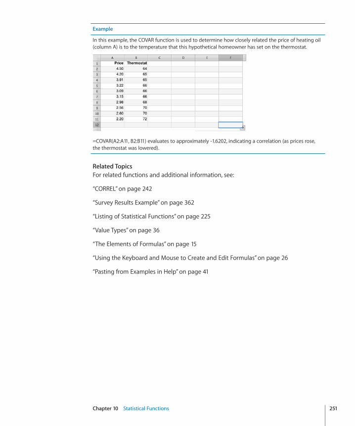
Chapter 10 Statistical Functions 251
Example
In this example, the COVAR function is used to determine how closely related the price of heating oil (column A) is to the temperature that this hypothetical homeowner has set on the thermostat.
=COVAR(A2:A11, B2:B11) evaluates to approximately -1.6202, indicating a correlation (as prices rose, the thermostat was lowered).
Related TopicsFor related functions and additional information, see:
“CORREL” on page 242
“Survey Results Example” on page 362
“Listing of Statistical Functions” on page 225
“Value Types” on page 36
“The Elements of Formulas” on page 15
“Using the Keyboard and Mouse to Create and Edit Formulas” on page 26
“Pasting from Examples in Help” on page 41

CRITBINOMThe CRITBINOM function returns the smallest value for which the cumulative binomial distribution is greater than or equal to a given value.
CRITBINOM(trials, prob-success, alpha)
 trials:� The total number of trials or tests. trials is a number value that must be greater than or equal to 0.
 prob-success:� The probability of success for each trial or test. prob-success is a number value that must be greater than or equal to 0 and less than or equal to 1.
 alpha:� The probability that the true population value lies outside the interval. alpha is a number value and must be less than or equal to 1. Subtracting the confidence interval from 1 yields the alpha.
Example
=CRITBINOM(97, 0.05, 0.05) returns 2, based on 97 trials, with each trial having a probability of success of 5% and a 95% confidence interval (5% alpha).
=CRITBINOM(97, 0.25, 0.1) returns 19, based on 97 trials, with each trial having a probability of success of 25% and a 90% confidence interval (10% alpha).
=CRITBINOM(97, 0.25, 0.05) returns 17, based on 97 trials, with each trial having a probability of success of 25% and a 95% confidence interval (5% alpha).
Related TopicsFor related functions and additional information, see:
“BINOMDIST” on page 238
“NEGBINOMDIST” on page 275
“PERMUT” on page 281
“PROB” on page 282
“Listing of Statistical Functions” on page 225
“Value Types” on page 36
“The Elements of Formulas” on page 15
“Using the Keyboard and Mouse to Create and Edit Formulas” on page 26
“Pasting from Examples in Help” on page 41
252 Chapter 10 Statistical Functions

Chapter 10 Statistical Functions 253
DEVSQThe DEVSQ function returns the sum of the squares of deviations of a collection of numbers from their average (arithmetic mean).
DEVSQ(num-value, num-value…)
 num-value:� A number. num-value is a number value.
 num-value…: Optionally include one or more additional numbers.
Usage NotesDEVSQ divides the sum of the numbers by the number of numbers to get the Âaverage (arithmetic mean). The difference (absolute value) between the average and each number is squared and summed and the total is returned.
Example
=DEVSQ(1, 7, 19, 8, 3, 9) returns 196.833333333333.
Related TopicsFor related functions and additional information, see:
“STDEV”
“Listing of Statistical Functions” on page 225
“Value Types” on page 36
“The Elements of Formulas” on page 15
“Using the Keyboard and Mouse to Create and Edit Formulas” on page 26
“Pasting from Examples in Help” on page 41
EXPONDISTThe EXPONDIST function returns the exponential distribution of the specified form.
EXPONDIST(non-neg-x-value, lambda, form-type)
 non-neg-x-value:� The value at which you want to evaluate the function. non-neg-x-value is a number value that must be greater than or equal to 0.
 lambda:� The parameter value. lambda is a number value and must be greater than 0.
 form-type:� A value that indicates which form of the exponential function to provide.
cumulative form (TRUE or 1):� Return the value of the cumulative distribution function form.
probability density form (FALSE or 0):� Return the value of the probability density function form.

Examples
=EXPONDIST(4, 2, 1) returns 0.999664537372097 (cumulative distribution form).
=EXPONDIST(4, 2, 0) returns 0.000670925255805024 (probability density form).
Related TopicsFor related functions and additional information, see:
“LOGNORMDIST” on page 269
“Listing of Statistical Functions” on page 225
“Value Types” on page 36
“The Elements of Formulas” on page 15
“Using the Keyboard and Mouse to Create and Edit Formulas” on page 26
“Pasting from Examples in Help” on page 41
FDISTThe FDIST function returns the F probability distribution.
FDIST(non-neg-x-value, d-f-numerator, d-f-denominator)
 non-neg-x-value:� The value at which you want to evaluate the function. non-neg-x-value is a number value that must be greater than or equal to 0.
 d-f-numerator:� The degrees of freedom to include as the numerator. d-f-numerator is a number value and must be greater than or equal to 1. If there is a decimal portion, it is ignored.
 d-f-denominator:� The degrees of freedom to include as the denominator. d-f-denominator is a number value and must be greater than or equal to 1. If there is a decimal portion, it is ignored.
Usage NotesThe F distribution is also known as Snedecor’s F distribution or the Fisher-Snedecor Âdistribution.
Examples
=FDIST(0.77, 1, 2) returns 0.472763488223567.
=FDIST(0.77, 1, 1) returns 0.541479597634413.
=FDIST(0.77, 2, 1) returns 0.627455805138159.
Related TopicsFor related functions and additional information, see:
254 Chapter 10 Statistical Functions

Chapter 10 Statistical Functions 255
“FINV” on page 255
“Listing of Statistical Functions” on page 225
“Value Types” on page 36
“The Elements of Formulas” on page 15
“Using the Keyboard and Mouse to Create and Edit Formulas” on page 26
“Pasting from Examples in Help” on page 41
FINVThe FINV function returns the inverse of the F probability distribution.
FINV(prob, d-f-numerator, d-f-denominator)
 prob:� A probability associated with the distribution. prob is a number value and must be greater than 0 and less than or equal to 1.
 d-f-numerator:� The degrees of freedom to include as the numerator. d-f-numerator is a number value and must be greater than or equal to 1. If there is a decimal portion, it is ignored.
 d-f-denominator:� The degrees of freedom to include as the denominator. d-f-denominator is a number value and must be greater than or equal to 1. If there is a decimal portion, it is ignored.
Examples
=FINV(0.77, 1, 2) returns 0.111709428782599.
=FINV(0.77, 1, 1) returns 0.142784612191674.
=FINV(0.77, 2, 1) returns 0.34331253162422.
Related TopicsFor related functions and additional information, see:
“FDIST” on page 254
“Listing of Statistical Functions” on page 225
“Value Types” on page 36
“The Elements of Formulas” on page 15
“Using the Keyboard and Mouse to Create and Edit Formulas” on page 26
“Pasting from Examples in Help” on page 41

FORECASTThe FORECAST function returns the forecasted y value for a given x based on sample values using linear regression analysis.
FORECAST(x-num-date-dur, y-values, x-values)
 x-num-date-dur:� The x value for which the function should return a forecasted y value. x-num-date-dur is a number value, a date/time value, or a duration value.
 y-values:� The collection containing the y (dependent) values. y-values is a collection that can contain number, date/time, or duration values. All values must be of the same type.
 x-values:� The collection containing the x (independent) values. x-values is a collection that can contain number, date/time, or duration values. All values must be of the same type.
Usage NotesAll arguments must be of the same type. Â
The two arrays must be of the same size. Â
If, for example, you had data on the driving speed of a vehicle and its fuel efficiency Âat each speed, fuel efficiency would be the dependent variable (y) and driving speed would be the independent variable (x).
You can use the SLOPE and INTERCEPT functions to find the equation used to Âcalculate forecast values.
Example
Given the following table:
=FORECAST(9, A3:F3, A2:F2) returns 19.
Related TopicsFor related functions and additional information, see:
“CORREL” on page 242
“COVAR” on page 250
“INTERCEPT” on page 262
“SLOPE” on page 287
“Listing of Statistical Functions” on page 225
256 Chapter 10 Statistical Functions

Chapter 10 Statistical Functions 257
“Value Types” on page 36
“The Elements of Formulas” on page 15
“Using the Keyboard and Mouse to Create and Edit Formulas” on page 26
“Pasting from Examples in Help” on page 41
FREQUENCYThe FREQUENCY function returns an array of how often data values occur within a range of interval values.
FREQUENCY(data-values, interval-values)
 data-values:� A collection containing the values to be evaluated. data-values is a collection containing number or date/time values. All values should be of the same type.
 interval-values:� A collection containing the interval values. interval-values is a collection containing number or date/time values. All values should be of the same type as the values in the data-values collection.
Usage NotesFREQUENCY determines the number of values in  data-values that fall within each interval. The interval array is easiest to understand if it is arranged in ascending order. The first frequency will be the count of those values that are less than or equal to the lowest interval value. All other frequency values, except the last, will be the count of those values that are greater than the immediately lower interval value and less than or equal to the current interval value. The final frequency value will be the count of those data values that are greater than the largest interval value.
The values returned by the function are contained in an array. One method of Âreading the values in the array is to use the INDEX function. You can wrap the FREQUENCY function within the INDEX function: =INDEX(FREQUENCY(data-values, interval-values), x) where x is the desired interval. Remember that there will be one more interval than there are interval-values.

Example
Assume the following table contains the test scores of 30 students who recently took an exam you administered. Assume further that that the minimum passing grade is 65 and that the lowest score for other grades are as given. In order to facilitate building the formulas, an “F” is represented by 1 and an “A” by 5.
=INDEX(FREQUENCY($A$1:$F$5, $B$8:$E$8), B9) returns 5, the number of students who received an “F” (score of 65 or less). This formula can be entered in cell B10 and then extended across to cell F10. The resulting values returned for grades of “D” to “A” are 3, 8, 8, and 6, respectively.
Related TopicsFor related functions and additional information, see:
“INDEX” on page 214
“PERCENTILE” on page 279
“PERCENTRANK” on page 280
“QUARTILE” on page 284
“Listing of Statistical Functions” on page 225
“Value Types” on page 36
“The Elements of Formulas” on page 15
“Using the Keyboard and Mouse to Create and Edit Formulas” on page 26
“Pasting from Examples in Help” on page 41
258 Chapter 10 Statistical Functions

Chapter 10 Statistical Functions 259
GAMMADISTThe GAMMADIST function returns the gamma distribution in the specified form.
GAMMADIST(non-neg-x-value, alpha, beta, form-type)
 non-neg-x-value:� The value at which you want to evaluate the function. non-neg-x-value is a number value that must be greater than or equal to 0.
 alpha:� One of the shape parameters of the distribution. alpha is a number value and must be greater than 0.
 beta:� One of the shape parameters of the distribution. beta is a number value and must be greater than 0.
 form-type:� A value that indicates which form of the exponential function to provide.
cumulative form (TRUE or 1):� Return the value of the cumulative distribution function form.
probability density form (FALSE or 0):� Return the value of the probability density function form.
Examples
=GAMMADIST(0.8, 1, 2, 1) returns 0.329679953964361 (the cumulative distribution form).
=GAMMADIST(0.8, 1, 2, 0) returns 0.33516002301782 (the probability density form).
Related TopicsFor related functions and additional information, see:
“GAMMAINV” on page 260
“GAMMALN” on page 260
“Listing of Statistical Functions” on page 225
“Value Types” on page 36
“The Elements of Formulas” on page 15
“Using the Keyboard and Mouse to Create and Edit Formulas” on page 26
“Pasting from Examples in Help” on page 41

GAMMAINVThe GAMMAINV function returns the inverse gamma cumulative distribution.
GAMMAINV(probability, alpha, beta)
 probability:� A probability associated with the distribution. probability is a number value and must be greater than 0 and less than 1.
 alpha:� One of the shape parameters of the distribution. alpha is a number value and must be greater than 0.
 beta:� One of the shape parameters of the distribution. beta is a number value and must be greater than 0.
Examples
=GAMMAINV(0.8, 1, 2) returns 3.2188758248682.
=GAMMAINV(0.8, 2, 1) returns 2.99430834700212.
Related TopicsFor related functions and additional information, see:
“GAMMADIST” on page 259
“GAMMALN” on page 260
“Listing of Statistical Functions” on page 225
“Value Types” on page 36
“The Elements of Formulas” on page 15
“Using the Keyboard and Mouse to Create and Edit Formulas” on page 26
“Pasting from Examples in Help” on page 41
GAMMALNThe GAMMALN function returns the natural logarithm of the gamma function, G(x).
GAMMALN(pos-x-value)
 pos-x-value:� The positive x value at which you want to evaluate the function. pos-x-value is a number value and must be greater than 0.
Examples
=GAMMALN(0.92) returns 0.051658003497744.
=GAMMALN(0.29) returns 1.13144836880416.
260 Chapter 10 Statistical Functions

Chapter 10 Statistical Functions 261
Related TopicsFor related functions and additional information, see:
“GAMMADIST” on page 259
“GAMMAINV” on page 260
“LN” on page 179
“Listing of Statistical Functions” on page 225
“Value Types” on page 36
“The Elements of Formulas” on page 15
“Using the Keyboard and Mouse to Create and Edit Formulas” on page 26
“Pasting from Examples in Help” on page 41
GEOMEANThe GEOMEAN function returns the geometric mean.
GEOMEAN(pos-num, pos-num…)
 pos-num:� A positive number. pos-num is a number value and must be greater than 0.
 pos-num…: Optionally include one or more additional positive numbers.
Usage NotesGEOMEAN multiples the arguments to arrive at a product and then takes the root of Âthe product that is equal to the number of arguments.
Example
=GEOMEAN(5, 7, 3, 2, 6, 22) returns 5.50130264578853.
Related TopicsFor related functions and additional information, see:
“AVERAGE” on page 231
“HARMEAN” on page 262
“Listing of Statistical Functions” on page 225
“Value Types” on page 36
“The Elements of Formulas” on page 15

“Using the Keyboard and Mouse to Create and Edit Formulas” on page 26
“Pasting from Examples in Help” on page 41
HARMEANThe HARMEAN function returns the harmonic mean.
HARMEAN(pos-num, pos-num…)
 pos-num:� A positive number. a-pos-num is a number value and must be greater than 0.
 pos-num…: Optionally include one or more additional positive numbers.
Usage NotesThe harmonic mean is the reciprocal of the arithmetic mean of the reciprocals. Â
Example
=HARMEAN(5, 7, 3, 2, 6, 22) returns 4.32179607109448.
Related TopicsFor related functions and additional information, see:
“AVERAGE” on page 231
“GEOMEAN” on page 261
“Listing of Statistical Functions” on page 225
“Value Types” on page 36
“The Elements of Formulas” on page 15
“Using the Keyboard and Mouse to Create and Edit Formulas” on page 26
“Pasting from Examples in Help” on page 41
INTERCEPTThe INTERCEPT function returns the y-intercept of the best-fit line for the collection using linear regression analysis.
INTERCEPT(y-values, x-numbers)
 y-values:� The collection containing the y (dependent) values. y-values is a collection that can contain number, date/time, or duration values. All values must be of the same type.
262 Chapter 10 Statistical Functions

Chapter 10 Statistical Functions 263
 x-numbers:� The collection containing the x (independent) values. x-numbers is a collection containing number values.
Usage NotesThe two arrays must be of the same size. Â
To find the slope of the best-fit line, use the SLOPE function. Â
Example
In this example, the INTERCEPT function is used to determine the y-intercept of the best-fit line for the temperature that this hypothetical homeowner has set on the thermostat (the dependent variable), based on the price of heating oil (the independent variable).
=INTERCEPT(B2:B11, A2:A11) evaluates to approximately 78, above the highest hypothetical value as the best-fit line sloping downward (as prices rose, the thermostat was lowered).
Related TopicsFor related functions and additional information, see:
“SLOPE” on page 287
“Listing of Statistical Functions” on page 225
“Value Types” on page 36
“The Elements of Formulas” on page 15
“Using the Keyboard and Mouse to Create and Edit Formulas” on page 26
“Pasting from Examples in Help” on page 41

LARGEThe LARGE function returns the nth-largest value within a collection. The largest value is ranked number 1.
LARGE(num-date-dur-set, ranking)
 num-date-dur-set:� A collection of values. num-date-dur-set is a collection containing number, date, or duration values. All values must be of the same type.
 ranking:� A number representing the size ranking of the value you want to retrieve. ranking is a number value and must be in the range of 1 to the number of values in the collection.
Usage NotesA ranking of 1 retrieves the largest number in the collection, 2 the second-largest, Âand so on. Values included in the array that are of the same size are ranked together, but impact the outcome.
Examples
Assume the following table contains the cumulative test scores for this semester for your 20 students. (We have organized the data this way for the example; it would likely originally have been in 20 separate rows.)
=LARGE(A1:E4, 1) returns 100, the largest cumulative test score (cell B2).
=LARGE(A1:E4, 2) returns 92, the second-largest cumulative test score (either cell B2 or cell C2).
=LARGE(A1:E4, 3) returns 92, also the third-largest cumulative test score as it appears twice (cells B2 and C2).
=LARGE(A1:E4, 6) returns 86, the sixth-largest cumulative test score (order is 100 , 92, 92, 91, 90, then 86).
Related TopicsFor related functions and additional information, see:
“RANK” on page 285
“SMALL” on page 288
“Listing of Statistical Functions” on page 225
“Value Types” on page 36
“The Elements of Formulas” on page 15
264 Chapter 10 Statistical Functions

Chapter 10 Statistical Functions 265
“Using the Keyboard and Mouse to Create and Edit Formulas” on page 26
“Pasting from Examples in Help” on page 41
LINESTThe LINEST function returns an array of the statistics for a straight line that best fits the given data using the “least squares” method.
LINEST(known-y-values, known-x-values, nonzero-y-intercept, more-stats)
 known-y-values:� The collection containing the known y values. known-y-values is a collection containing number values. If there is only one collection of known x values, known-y-values can be any size. If there is more than one collection of known x values, known-y-values can be either one column containing the values or one row containing the values, but not both.
 known-x-values:� An optional collection containing the known x values. known-x-values is a collection containing number values. If omitted, it will be assumed to be the set {1, 2, 3…} of the same size as known-y-values. If there is only one set of known x values, known-x-values, if specified, should be the same size as known-y-values. If there is more than one set of known x values, each row/column of known-x-values is considered to be one set and the size of each row/column must be the same as the size of the row/column of known-y-values.
 nonzero-y-intercept:� An optional value specifying how the y intercept (constant b) should be calculated.
normal (1, TRUE, or omitted):� The value of the y intercept (constant b) should be calculated normally.
force 0 value (0, FALSE):� The value of the y intercept (constant b) should be forced to be 0.
 more-stats:� An optional value specifying whether additional statistical information should be returned.
no additional stats (0, FALSE, or omitted):� Do not return additional regression statistics in the returned array.
additional stats (1, TRUE):� Return additional regression statistics in the returned array.
Usage NotesThe values returned by the function are contained in an array. One method of Âreading the values in the array is to use the INDEX function. You can wrap the LINEST function within the INDEX function: =INDEX(LINEST(known-y-values, known-x-values, const-b, stats), y, x) where y and x are the column and row index of the desired value.

If additional statistics are not returned (stats is FALSE), the array returned is one row deep. The number of columns is equal to the the number of sets of known-x-values plus 1. It contains the line slopes (one value for each row/column of x values) in reverse order (the first value relates to the last row/column of x values) and then the value for b, the intercept.
If additional statistics are returned (stats is TRUE), the array contains five rows. See “Additional Statistics” on page 267 for the contents of the array.
Examples
Assume the following table contains the test scores of 30 students who recently took an exam you administered. Assume further that the minimum passing grade is 65 and that the lowest score for other grades are as given. In order to facilitate building the formulas, an “F” is represented by 1 and an “A” by 5.
=INDEX(LINEST(A2:A6, C2:C6, 1, 0), 1) returns 0.752707581227437, which is the best-fit line slope.
=INDEX(LINEST(A2:A6, C2:C6, 1, 0), 2) returns 0.0342960288808646, which is b, the intercept.
Related TopicsFor related functions and additional information, see:
“Listing of Statistical Functions” on page 225
“Value Types” on page 36
“The Elements of Formulas” on page 15
“Using the Keyboard and Mouse to Create and Edit Formulas” on page 26
“Pasting from Examples in Help” on page 41
266 Chapter 10 Statistical Functions

Chapter 10 Statistical Functions 267
Additional StatisticsThis section discusses the additional statistics that can be returned by the LINEST function.
LINEST can include additional statistical information in the array returned by the function. For purposes of the following discussion, assume that there are five sets of known x values, in addition to the known y values. Assume further that the known x values are in five table rows or five table columns. Based on these assumptions, the array returned by LINEST would be as follows (where the number following an x indicates which set of x values the item refers to):
Row/Column 1 2 3 4 5 6
1 slope x5 slope x4 slope x3 slope x2 slope x1 b (y intercept)
2 std-err x1 std-err x2 std-err x3 std-err x4 std-err x5 std-err b
3 coefficient-det std-err y
4 F-stat degrees-of-freedom
5 reg-ss reside-ss
Argument definitionsslope x:� The slope of the line related to this set of known x values. The values are returned in reverse order; that is, if there are five known x value sets, the value for the fifth set is first in the returned array.
b:� The y intercept for the known x values.
std-err x:� The standard error for the coefficient associated with this set of known x values. The values are returned in order; that is, if there are five known x value sets, the value for the first set is returned first in the array. This is the opposite of the way the slope values are returned.
std-err b:� The standard error associated with the y-intercept value (b).
coefficient-det: The coefficient of determination. This statistic compares estimated and actual y values. If it is 1, there is no difference between the estimated y value and the actual y value. This is known as perfect correlation. If the coefficient of determination is 0, there is no correlation and the given regression equation is not helpful in predicting a y value.
std-err y:� The standard error associated with the y value estimate.
F-stat:� The F observed value. The F observed value can be used to help determine whether the observed relationship between the dependent and independent variables occurs by chance.
degrees-of-freedom:� The degrees of freedom. Use the degrees of freedom statistic to help determine a confidence level.

reg-ss:� The regression sum of squares.
reside-ss:� The residual sum of squares.
Usage NotesIt does not matter whether the known x values and known y values are in rows or Âcolumns. In either case, the returned array is ordered by rows as illustrated in the table.
The example assumed five sets of known x values. If there were more or less than Âfive, the number of columns in the returned array would change accordingly (it is always equal to the number of sets of known x values plus 1), but the number of rows would remain constant.
If additional statistics are not specified in the arguments to LINEST, the returned Âarray is equal to the first row only.
LOGINVThe LOGINV function returns the inverse of the log-normal cumulative distribution function of x.
LOGINV(probability, mean, stdev)
 probability:� A probability associated with the distribution. probability is a number value and must be greater than 0 and less than 1.
 mean:� The mean of the natural logarithm, that is, ln(x)
. mean is a number value and is the average (arithmetic mean) of ln
(x); the natural logarithm of x.
 stdev:� The standard deviation of the population. stdev is a number value and must be greater than 0.
Usage NotesLOGINV is appropriate where the logarithm of x is normally distributed. Â
Example
=LOGINV(0.78, 1.7, 2.2) returns 29.9289150377259.
Related TopicsFor related functions and additional information, see:
“LN” on page 179
“LOGNORMDIST” on page 269
“Listing of Statistical Functions” on page 225
“Value Types” on page 36
268 Chapter 10 Statistical Functions

Chapter 10 Statistical Functions 269
“The Elements of Formulas” on page 15
“Using the Keyboard and Mouse to Create and Edit Formulas” on page 26
“Pasting from Examples in Help” on page 41
LOGNORMDISTThe LOGNORMDIST function returns the log-normal distribution.
LOGNORMDIST(pos-x-value, mean, stdev)
 pos-x-value:� The positive x value at which you want to evaluate the function. pos-x-value is a number value that must be greater than 0.
 mean:� The mean of the natural logarithm, that is, ln(x)
. mean is a number value and is the average (arithmetic mean) of ln
(x); the natural logarithm of x.
 stdev:� The standard deviation of the population. stdev is a number value and must be greater than 0.
Example
=LOGNORMDIST(0.78, 1.7, 2.2) returns 0.187899237956868.
Related TopicsFor related functions and additional information, see:
“LN” on page 179
“LOGINV” on page 268
“Listing of Statistical Functions” on page 225
“Value Types” on page 36
“The Elements of Formulas” on page 15
“Using the Keyboard and Mouse to Create and Edit Formulas” on page 26
“Pasting from Examples in Help” on page 41

MAXThe MAX function returns the largest number in a collection.
MAX(value, value…)
 value:� A value. value can contain any value type.
 value…: Optionally include one or more additional values.
Usage NotesIf  value does not evaluate to a date or number, it is not included in the result.
To determine the largest of any type of value in a collection, use the MAXA function. Â
Examples
=MAX(5, 5, 5, 5, 6) returns 6.
=MAX(1, 2, 3, 4, 5) returns 5.
Related TopicsFor related functions and additional information, see:
“LARGE” on page 264
“MAXA” on page 270
“MIN” on page 272
“SMALL” on page 288
“Listing of Statistical Functions” on page 225
“Value Types” on page 36
“The Elements of Formulas” on page 15
“Using the Keyboard and Mouse to Create and Edit Formulas” on page 26
“Pasting from Examples in Help” on page 41
MAXAThe MAXA function returns the largest number in a collection of values that may include text and Boolean values.
MAXA(value, value…)
 value:� A value. value can contain any value type.
 value…: Optionally include one or more additional values. All numeric values must be of the same type. You cannot mix numbers, dates, and duration values.
270 Chapter 10 Statistical Functions

Chapter 10 Statistical Functions 271
Usage NotesText values and logical FALSE are given a value of 0 and logical TRUE is given a value Âof 1.
To determine the largest value of a collection that contains only numbers or dates, Âuse the MAX function.
Examples
=MAXA(1, 2, 3, 4) returns 4.
=MAXA(A1:C1), where A1:C1 contains -1, -10, hello, returns 0.
Related TopicsFor related functions and additional information, see:
“MAX” on page 270
“MINA” on page 273
“Listing of Statistical Functions” on page 225
“Value Types” on page 36
“The Elements of Formulas” on page 15
“Using the Keyboard and Mouse to Create and Edit Formulas” on page 26
“Pasting from Examples in Help” on page 41
MEDIANThe MEDIAN function returns the median value in a collection of numbers. The median is the value where half the numbers in the set are less than the median and half are greater.
MEDIAN(num-date-dur, num-date-dur…)
 num-date-dur:� A value. num-date-dur is a number value, a date/time value, or a duration value.
 num-date-dur…: Optionally include one or more additional values. If more than one num-date-dur value is specified, all must be of the same type.
Usage NotesIf there is an even number of values in the set, the MEDIAN function returns the Âaverage of the two middle values.

Examples
=MEDIAN(1, 2, 3, 4, 5) returns 3.
=MEDIAN(1, 2, 3, 4, 5, 6) returns 3.5.
=MEDIAN(5, 5, 5, 5, 6) returns 5.
Related TopicsFor related functions and additional information, see:
“AVERAGE” on page 231
“MODE” on page 274
“Listing of Statistical Functions” on page 225
“Value Types” on page 36
“The Elements of Formulas” on page 15
“Using the Keyboard and Mouse to Create and Edit Formulas” on page 26
“Pasting from Examples in Help” on page 41
MINThe MIN function returns the smallest number in a collection.
MIN(value, value…)
 value:� A value. value can contain any value type.
 value…: Optionally include one or more additional values.
Usage NotesIf  value does not evaluate to a date or number, it is not included in the result.
To determine the smallest of any type of value in a collection, use the MINA Âfunction.
Examples
=MIN(5, 5, 5, 5, 6) returns 5.
=MIN(1, 2, 3, 4, 5) returns 1.
Related TopicsFor related functions and additional information, see:
“LARGE” on page 264
“MAX” on page 270
272 Chapter 10 Statistical Functions

Chapter 10 Statistical Functions 273
“MINA” on page 273
“SMALL” on page 288
“Listing of Statistical Functions” on page 225
“Value Types” on page 36
“The Elements of Formulas” on page 15
“Using the Keyboard and Mouse to Create and Edit Formulas” on page 26
“Pasting from Examples in Help” on page 41
MINAThe MINA function returns the smallest number in a collection of values that may include text and Boolean values.
MINA(value, value…)
 value:� A value. value can contain any value type.
 value…: Optionally include one or more additional values. All numeric values must be of the same type. You cannot mix numbers, dates, and duration values.
Usage NotesText values and logical FALSE are given a value of 0 and logical TRUE is given a value Âof 1.
To determine the smallest value of a collection that contains only numbers or dates, Âuse the MIN function.
Examples
=MINA(1, 2, 3, 4) returns 1.
=MINA(A1:C1), where A1:C1 contains -1, -10, hello, returns -10.
=MINA(A1:C1), where A1:C1 contains 1, 10, hello, returns 0.
Related TopicsFor related functions and additional information, see:
“MAXA” on page 270
“MIN” on page 272
“Listing of Statistical Functions” on page 225
“Value Types” on page 36
“The Elements of Formulas” on page 15

“Using the Keyboard and Mouse to Create and Edit Formulas” on page 26
“Pasting from Examples in Help” on page 41
MODEThe MODE function returns the most frequently occurring value in a collection of numbers.
MODE(num-date-dur, num-date-dur…)
 num-date-dur:� A value. num-date-dur is a number value, a date/time value, or a duration value.
 num-date-dur…: Optionally include one or more additional values. If more than one num-date-dur value is specified, all must be of the same type.
Usage NotesIf more than one number occurs the maximum multiple times in the arguments, ÂMODE returns the first such number.
If no value occurs more than once, the function returns an error. Â
Examples
=MODE(5, 5, 5, 5, 6) returns 5.
=MODE(1, 2, 3, 4, 5) returns an error.
=MODE(2, 2, 4, 6, 6) returns 2.
=MODE(6, 6, 4, 2, 2) returns 6.
Related TopicsFor related functions and additional information, see:
“AVERAGE” on page 231
“MEDIAN” on page 271
“Listing of Statistical Functions” on page 225
“Value Types” on page 36
“The Elements of Formulas” on page 15
“Using the Keyboard and Mouse to Create and Edit Formulas” on page 26
“Pasting from Examples in Help” on page 41
274 Chapter 10 Statistical Functions

Chapter 10 Statistical Functions 275
NEGBINOMDISTThe NEGBINOMDIST function returns the negative binomial distribution.
NEGBINOMDIST(f-num, s-num, prob-success)
 f-num:� The number of failures. f-num is a number value and must be greater than or equal to 0.
 s-num:� The number of successful trials or tests. s-num is a number value that must be greater than or equal to 1.
 prob-success:� The probability of success for each trial or test. prob-success is a number value that must be greater than 0 and less than 1.
Usage NotesNEGBINOMDIST returns the probability that there will be a specified number of Âfailures, f-num, before the specified number of successes, s-num. The constant probability of a success is prob-success.
Example
=NEGBINOMDIST(3, 68, 0.95) returns 0.20913174716192.
Related TopicsFor related functions and additional information, see:
“BINOMDIST” on page 238
“CRITBINOM” on page 252
“PERMUT” on page 281
“PROB” on page 282
“Listing of Statistical Functions” on page 225
“Value Types” on page 36
“The Elements of Formulas” on page 15
“Using the Keyboard and Mouse to Create and Edit Formulas” on page 26
“Pasting from Examples in Help” on page 41

NORMDISTThe NORMDIST function returns the normal distribution of the specified function form.
NORMDIST(num, average, stdev, form-type)
 num:� The number to be evaluated. num is a number value.
 average:� The average of the distribution. average is a number value representing the known average (arithmetic mean) rate at which events occur.
 stdev:� The standard deviation of the population. stdev is a number value and must be greater than 0.
 form-type:� A value that indicates which form of the exponential function to provide.
cumulative form (TRUE or 1):� Return the value of the cumulative distribution function form.
probability density form (FALSE or 0):� Return the value of the probability density function form.
Usage NotesIf  average is 0, stdev is 1, and form-type is TRUE, NORMDIST returns the same value as the cumulative standard normal distribution returned by NORMSDIST.
Examples
=NORMDIST(22, 15, 2.5, 1) returns 0.997444869669572, the cumulative distribution form.
=NORMDIST(22, 15, 2.5, 0) returns 0.00316618063319199, the probability density form.
Related TopicsFor related functions and additional information, see:
“NORMINV” on page 277
“NORMSDIST” on page 277
“Listing of Statistical Functions” on page 225
“Value Types” on page 36
“The Elements of Formulas” on page 15
“Using the Keyboard and Mouse to Create and Edit Formulas” on page 26
“Pasting from Examples in Help” on page 41
276 Chapter 10 Statistical Functions

Chapter 10 Statistical Functions 277
NORMINVThe NORMINV function returns the inverse of the cumulative normal distribution.
NORMINV(probability, average, stdev)
 probability:� A probability associated with the distribution. probability is a number value and must be greater than 0 and less than 1.
 average:� The average of the distribution. average is a number value representing the known average (arithmetic mean) rate at which events occur.
 stdev:� The standard deviation of the population. stdev is a number value and must be greater than 0.
Usage NotesIf  average is 0 and stdev is 1, NORMINV returns the same value as the inverse of the cumulative standard normal distribution returned by NORMSINV.
Example
=NORMINV(0.89, 15, 2.5) returns 18.0663203000915.
Related TopicsFor related functions and additional information, see:
“NORMDIST” on page 276
“NORMSINV” on page 278
“Listing of Statistical Functions” on page 225
“Value Types” on page 36
“The Elements of Formulas” on page 15
“Using the Keyboard and Mouse to Create and Edit Formulas” on page 26
“Pasting from Examples in Help” on page 41
NORMSDISTThe NORMSDIST function returns the standard normal distribution.
NORMSDIST(num)
 num:� A number. num is a number value.
Usage NotesA standard normal distribution has an average (arithmetic mean) of 0 and a Âstandard deviation of 1.

Example
=NORMSDIST(4.3) returns 0.999991460094529.
Related TopicsFor related functions and additional information, see:
“NORMDIST” on page 276
“NORMSINV” on page 278
“Listing of Statistical Functions” on page 225
“Value Types” on page 36
“The Elements of Formulas” on page 15
“Using the Keyboard and Mouse to Create and Edit Formulas” on page 26
“Pasting from Examples in Help” on page 41
NORMSINVThe NORMSINV function returns the inverse of the cumulative standard normal distribution.
NORMSINV(probability)
 probability:� A probability associated with the distribution. probability is a number value and must be greater than 0 and less than 1.
Usage NotesA standard normal distribution has an average (arithmetic mean) of 0 and a Âstandard deviation of 1.
Example
=NORMSINV(0.89) returns 1.22652812003661.
Related TopicsFor related functions and additional information, see:
“NORMINV” on page 277
“NORMSDIST” on page 277
“Listing of Statistical Functions” on page 225
“Value Types” on page 36
278 Chapter 10 Statistical Functions

Chapter 10 Statistical Functions 279
“The Elements of Formulas” on page 15
“Using the Keyboard and Mouse to Create and Edit Formulas” on page 26
“Pasting from Examples in Help” on page 41
PERCENTILEThe PERCENTILE function returns the value within a collection that corresponds to a particular percentile.
PERCENTILE(num-date-dur-set, percentile-value)
 num-date-dur-set:� A collection of values. num-date-dur-set is a collection containing number, date, or duration values. All values must be of the same type.
 percentile-value:� The percentile value you want to find, in the range 0 to 1. percentile-value is a number value and is either entered as a decimal (for example, 0.25) or delimited with a percent sign (for example, 25%). It must be greater than or equal to 0 and less than or equal to 1.
Usage NotesValues included in the array of the same size are ranked together, but impact the Âoutcome.
Examples
Assume the following table contains the cumulative test scores for this semester for your 20 students. (We have organized the data this way for the example; it would likely originally have been in 20 separate rows.)
=PERCENTILE(A1:E4, 0.90) returns 92, the minimum cumulative test score to be in the top 10% of the class (90th percentile).
=PERCENTILE(A1:E4, 2/3) returns 85, the minimum cumulative test score to be in the top one-third of the class (2/3 or approximately 67th percentile).
=PERCENTILE(A1:E4, 0.50) returns 83, the minimum cumulative test score to be in the top half of the class (the 50th percentile).
Related TopicsFor related functions and additional information, see:
“FREQUENCY” on page 257
“PERCENTRANK” on page 280

“QUARTILE” on page 284
“Listing of Statistical Functions” on page 225
“Value Types” on page 36
“The Elements of Formulas” on page 15
“Using the Keyboard and Mouse to Create and Edit Formulas” on page 26
“Pasting from Examples in Help” on page 41
PERCENTRANKThe PERCENTRANK function returns the rank of a value in a collection as a percentage of the collection.
PERCENTRANK(num-date-dur-set, num-date-dur, significance)
 num-date-dur-set:� A collection of values. num-date-dur-set is a collection containing number, date, or duration values. All values must be of the same type.
 num-date-dur:� A value. num-date-dur is a number value, a date/time value, or a duration value.
 significance: An optional value specifying the number of digits to the right of the decimal point. significance is a number value that must be greater than or equal to 1. If omitted, a default value of 3 is used (x.xxx%).
Usage NotesPERCENTRANK can be used to evaluate the relative standing of a value within Âa collection. It is calculated by determining where in the collection a specified number falls. For example, if in a given collection, there are ten values smaller than a specified number and ten values that are larger, the PERCENTRANK of the specified number is 50%.
Example
=PERCENTRANK({5, 6, 9, 3, 7, 11, 8, 2, 14}, 10) returns 0.813, as there are seven values smaller than 10 and only two that are larger.
Related TopicsFor related functions and additional information, see:
“FREQUENCY” on page 257
“PERCENTILE” on page 279
“Listing of Statistical Functions” on page 225
280 Chapter 10 Statistical Functions

Chapter 10 Statistical Functions 281
“Value Types” on page 36
“The Elements of Formulas” on page 15
“Using the Keyboard and Mouse to Create and Edit Formulas” on page 26
“Pasting from Examples in Help” on page 41
PERMUTThe PERMUT function returns the number of permutations for a given number of objects that can be selected from a total number of objects.
PERMUT(num-objects, num-elements)
 num-objects:� The total number of objects. num-objects is a number value and must be greater than or equal to 0.
 num-elements:� The number of objects to be selected from the total number of objects in each permutation. num-elements is a number value and must be greater than or equal to 0.
Examples
=PERMUT(25, 5) returns 6375600.
=PERMUT(10, 3) returns 720.
=PERMUT(5, 2) returns 20.
Related TopicsFor related functions and additional information, see:
“BINOMDIST” on page 238
“CRITBINOM” on page 252
“NEGBINOMDIST” on page 275
“PROB” on page 282
“Listing of Statistical Functions” on page 225
“Value Types” on page 36
“The Elements of Formulas” on page 15
“Using the Keyboard and Mouse to Create and Edit Formulas” on page 26
“Pasting from Examples in Help” on page 41
POISSONThe POISSON function returns the probability that a specific number of events will occur using the Poisson distribution.
POISSON(events, average, form-type)
 events:� The number of events (arrivals) for which you want to calculate the probability. events is a number value.
 average:� The average of the distribution. average is a number value representing the known average (arithmetic mean) rate at which events occur.
 form-type:� A value that indicates which form of the exponential function to provide.
cumulative form (TRUE or 1):� Return the value of the cumulative distribution function form (that the specified number or fewer successes or events will occur).
probability mass form (FALSE or 0):� Return the value of the probability mass function form (that there are exactly the specified number of successes or events).
Example
For a mean of 10 and an arrival rate of 8:
=POISSON(8, 10, FALSE) returns 0.112599.
Related TopicsFor related functions and additional information, see:
“EXPONDIST” on page 253
“Listing of Statistical Functions” on page 225
“Value Types” on page 36
“The Elements of Formulas” on page 15
“Using the Keyboard and Mouse to Create and Edit Formulas” on page 26
“Pasting from Examples in Help” on page 41
PROBThe PROB function returns the probability of a range of values if you know the probabilities of the individual values.
PROB(num-set, probability-values, lower, upper)
 num-set:� A collection of numbers. num-set is a collection containing number values.
282 Chapter 10 Statistical Functions

Chapter 10 Statistical Functions 283
 probability-values:� The collection containing the probability values. probability-values is a collection containing number values. The sum of the probabilities must add up to 1. Any string values are ignored.
 lower:� The lower limit or bound. lower is a number value.
 upper:� An optional upper limit or bound. upper is a number value and must be greater than or equal to lower.
Usage NotesThe PROB function sums the probabilities associated with all values in the collection Âgreater than or equal to the specified lower limit value and less than or equal to the specified upper limit value. If upper is omitted, PROB returns the probability of the single number equal to the specified lower limit.
The two arrays must be of the same size. If text is contained in an array, it will be Âignored.
Examples
Assume you are thinking of a number from 1 to 10 to have someone guess. Most people would say the probability that you would be thinking of a particular number is 0.1 (10%), as listed in column C, since there are ten possible choices. However, studies have shown that people do not choose numbers randomly.
Assume that a study has shown that people like you are more likely to select certain numbers than others. These revised probabilities are in column E.
=PROB(A1:A10, C1:C10, 4, 6) returns 0.30, the probability that the value is 4, 5, or 6, assuming choices are completely random.
=PROB(A1:A10, E1:E10, 7) returns 0.28, the probability that the value is 4, 5, or 6, based on the research that numbers are not chosen randomly.
=PROB(A1:A10, E1:E10, 4, 6) returns 0.20, the probability that the value is 7, based on the research that numbers are not chosen randomly.
=PROB(A1:A10, C1:C10, 6, 10) returns 0.50, the probability that the value is greater than 5 (6 to 10), assuming choices are completely random.

Related TopicsFor related functions and additional information, see:
“BINOMDIST” on page 238
“CRITBINOM” on page 252
“NEGBINOMDIST” on page 275
“PERMUT” on page 281
“Listing of Statistical Functions” on page 225
“Value Types” on page 36
“The Elements of Formulas” on page 15
“Using the Keyboard and Mouse to Create and Edit Formulas” on page 26
“Pasting from Examples in Help” on page 41
QUARTILEThe QUARTILE function returns the value for the specified quartile of a given data collection.
QUARTILE(num-set, quartile-num)
 num-set:� A collection of numbers. num-set is a collection containing number values.
 quartile-num:� Specifies the desired quartile.
smallest (0):� Returns the smallest value.
first (1): Returns the first quartile (25th percentile).
second (2):� Returns the second quartile (50th percentile).
third (3):� Returns the third quartile (75th percentile).
largest (4):� Returns the largest value.
Usage NotesMIN, MEDIAN, and MAX return the same value as QUARTILE when  quartile-num is equal to 0, 2, and 4, respectively.
284 Chapter 10 Statistical Functions

Chapter 10 Statistical Functions 285
Examples
=QUARTILE({5, 6, 9, 3, 7, 11, 8, 2, 14}, 0) returns 2, the smallest value.
=QUARTILE({5, 6, 9, 3, 7, 11, 8, 2, 14}, 1) returns 5, the 25th percentile or first quartile.
=QUARTILE({5, 6, 9, 3, 7, 11, 8, 2, 14}, 2) returns 7, the 50th percentile or second quartile.
=QUARTILE({5, 6, 9, 3, 7, 11, 8, 2, 14}, 3) returns 9, the 75th percentile or third quartile.
=QUARTILE({5, 6, 9, 3, 7, 11, 8, 2, 14}, 0) returns 14, the largest value.
Related TopicsFor related functions and additional information, see:
“FREQUENCY” on page 257
“MAX” on page 270
“MEDIAN” on page 271
“MIN” on page 272
“PERCENTILE” on page 279
“PERCENTRANK” on page 280
“Listing of Statistical Functions” on page 225
“Value Types” on page 36
“The Elements of Formulas” on page 15
“Using the Keyboard and Mouse to Create and Edit Formulas” on page 26
“Pasting from Examples in Help” on page 41
RANKThe RANK function returns the rank of a number within a range of numbers.
RANK(num-date-dur, num-date-dur-set, largest-is-high)
 num-date-dur:� A value. num-date-dur is a number value, a date/time value, or a duration value.
 num-date-dur-set:� A collection of values. num-date-dur-set is a collection containing number, date, or duration values. All values must be of the same type.

 largest-is-high:� An optional value specifying whether the smallest or the largest value in the collection is ranked 1.
largest is low (0, FALSE, or omitted):� Assign the largest value in the collection the rank 1.
largest is high (1, or TRUE):� Assign the smallest value in the collection the rank 1.
Usage NotesValues included in the collection that are the same are ranked together, but impact Âthe outcome.
If the specified value does not match any of the values in the collection, an error is Âreturned.
Examples
Assume the following table contains the cumulative test scores for this semester for your 20 students. (We have organized the data this way for the example; it would likely originally have been in 20 separate rows.)
=RANK(30, A1:E4, 1) returns 1, as 30 is the smallest cumulative test score and we chose to rank the smallest first.
=RANK(92, A1:E4, 0) returns 2, as 92 is the second-largest cumulative test score and we chose to rank largest first.
=RANK(91, A1:E4, 1) returns 4, as there is a “tie” for second place. The order is 100, 92, 92, then 91 and the rank is 1, 2, 2, and then 4.
Related TopicsFor related functions and additional information, see:
“LARGE” on page 264
“SMALL” on page 288
“Listing of Statistical Functions” on page 225
“Value Types” on page 36
“The Elements of Formulas” on page 15
“Using the Keyboard and Mouse to Create and Edit Formulas” on page 26
“Pasting from Examples in Help” on page 41
286 Chapter 10 Statistical Functions

Chapter 10 Statistical Functions 287
SLOPEThe SLOPE function returns the slope of the best-fit line for the collection using linear regression analysis.
SLOPE(y-values, x-values)
 y-values:� The collection containing the y (dependent) values. y-values is a collection that can contain number, date/time, or duration values. All values must be of the same type.
 x-values:� The collection containing the x (independent) values. x-values is a collection that can contain number, date/time, or duration values. All values must be of the same type.
Usage NotesThe two collections must be of the same size or the function returns an error. Â
If, for example, you had data on the driving speed of a vehicle and its fuel efficiency Âat each speed, fuel efficiency would be the dependent variable and driving speed would be the independent variable.
To find the y-intercept of the best-fit line, use the INTERCEPT function. Â
Example
In this example, the SLOPE function is used to determine the slope of the best-fit line for the temperature that this hypothetical homeowner has set on the thermostat (the dependent variable), based on the price of heating oil (the independent variable).
=SLOPE(B2:B11, A2:A11) evaluates to approximately -3.2337, indicating a best-fit line sloping downward (as prices rose, the thermostat was lowered).
Related TopicsFor related functions and additional information, see:
“INTERCEPT” on page 262
“Listing of Statistical Functions” on page 225
“Value Types” on page 36

“The Elements of Formulas” on page 15
“Using the Keyboard and Mouse to Create and Edit Formulas” on page 26
“Pasting from Examples in Help” on page 41
SMALLThe SMALL function returns the nth-smallest value within a range. The smallest value is ranked number 1.
SMALL(num-date-dur-set, ranking)
 num-date-dur-set:� A collection of values. num-date-dur-set is a collection containing number, date, or duration values. All values must be of the same type.
 ranking:� A number representing the size ranking of the value you want to retrieve. ranking is a number value and must be in the range of 1 to the number of values in the collection.
Usage NotesA ranking of 1 retrieves the smallest number in the collection, 2 the second-smallest, Âand so on. Values included in the collection that are of the same size are ranked together, but impact the outcome.
Examples
Assume the following table contains the cumulative test scores for this semester for your 20 students. (We have organized the data this way for the example; it would likely originally have been in 20 separate rows.)
=SMALL(A1:E4, 1) returns 30, the smallest cumulative test score (cell A1).
=SMALL(A1:E4, 2) returns 51, the second-smallest cumulative test score (cell E1).
=SMALL(A1:E4, 6) returns 75, the sixth-smallest cumulative test score (order is 30, 51, 68, 70, 75, then 75 again, so 75 is both the fifth- and sixth-smallest cumulative test score).
Related TopicsFor related functions and additional information, see:
“LARGE” on page 264
“RANK” on page 285
“Listing of Statistical Functions” on page 225
288 Chapter 10 Statistical Functions

Chapter 10 Statistical Functions 289
“Value Types” on page 36
“The Elements of Formulas” on page 15
“Using the Keyboard and Mouse to Create and Edit Formulas” on page 26
“Pasting from Examples in Help” on page 41
STANDARDIZEThe STANDARDIZE function returns a normalized value from a distribution characterized by a given mean and standard deviation.
STANDARDIZE(num, average, stdev)
 num:� The number to be evaluated. num is a number value.
 average:� The average of the distribution. average is a number value representing the known average (arithmetic mean) rate at which events occur.
 stdev:� The standard deviation of the population. stdev is a number value and must be greater than 0.
Example
=STANDARDIZE(6, 15, 2.1) returns –4.28571428571429.
Related TopicsFor related functions and additional information, see:
“NORMDIST” on page 276
“NORMINV” on page 277
“NORMSDIST” on page 277
“NORMSINV” on page 278
“ZTEST” on page 305
“Listing of Statistical Functions” on page 225
“Value Types” on page 36
“The Elements of Formulas” on page 15
“Using the Keyboard and Mouse to Create and Edit Formulas” on page 26
“Pasting from Examples in Help” on page 41

STDEVThe STDEV function returns the standard deviation, a measure of dispersion, of a collection of values based on their sample (unbiased) variance.
STDEV(num-date-dur, num-date-dur…)
 num-date-dur:� A value. num-date-dur is a number value, a date/time value, or a duration value.
 num-date-dur…: One or more additional values (a minimum of two values are required). All num-date-dur values must be of the same type.
Usage NotesIt is appropriate to use STDEV when the specified values represent only a sample of Âa larger population. If the values you are analyzing represent the entire collection or population, use the STDEVP function.
If you want to include text or Boolean values in the computation, use the STDEVA Âfunction.
The standard deviation is the square root of the variance returned by the VAR Âfunction.
Example
Assume you have administered five tests to a group of students. You have arbitrarily selected five students to represent the total population of students (note that this is an example only; this would not likely be statistically valid). Using the sample data, you could use the STDEV function to determine which test had the widest dispersion of test scores.
The results of the STDEV functions are approximately 22.8035, 24.5357, 9.5026, 8.0747, and 3.3466. So test 2 had the highest dispersion, followed closely by test 1. The other three tests had low dispersion.
Test 1 Test 2 Test 3 Test 4 Test 5
Student 1 75 82 90 78 84
Student 2 100 90 95 88 90
Student 3 40 80 78 90 85
Student 4 80 35 95 98 92
Student 5 90 98 75 97 88
=STDEV(B2:B6) =STDEV(C2:C6) =STDEV(D2:D6) =STDEV(E2:E6) =STDEV(F2:F6)
Related TopicsFor related functions and additional information, see:
“STDEVA” on page 291
“STDEVP” on page 293
290 Chapter 10 Statistical Functions

Chapter 10 Statistical Functions 291
“STDEVPA” on page 294
“VAR” on page 298
“VARA” on page 300
“VARP” on page 302
“VARPA” on page 303
“Survey Results Example” on page 362
“Listing of Statistical Functions” on page 225
“Value Types” on page 36
“The Elements of Formulas” on page 15
“Using the Keyboard and Mouse to Create and Edit Formulas” on page 26
“Pasting from Examples in Help” on page 41
STDEVAThe STDEVA function returns the standard deviation, a measure of dispersion, of a collection of values that may include text and Boolean values, based on the sample (unbiased) variance.
STDEVA(value, value…)
 value:� A value. value can contain any value type. All numeric values must be of the same type. You cannot mix numbers, dates, and duration values.
 value…: One or more additional values (a minimum of two values are required). All numeric values must be of the same type. You cannot mix numbers, dates, and duration values.
Usage NotesIt is appropriate to use STDEVA when the specified values represent only a sample Âof a larger population. If the values you are analyzing represent the entire collection or population, use the STDEVPA function.
STDEVA assigns a value of 0 to any text value, 0 to the Boolean value FALSE, and 1 Âto the Boolean value TRUE and includes them in the computation. Empty cells are ignored. If you do not want to include text or Boolean values in the computation, use the STDEV function.
The standard deviation is the square root of the variance returned by the VARA function. Â

Example
Assume you have installed a temperature sensor in Cupertino, California. The sensor records each day’s high and low temperatures. In addition, you have kept a record of each day you turned on the air conditioner in your condo. The data from the first few days is shown in the following table and is used as a sample for the population of high and low temperatures (note that this is an example only; this would not be statistically valid).
=STDEVA(B2:B13) returns 24.8271, the dispersion as measured by STDEVA, of the sample of daily high temperatures.
It exceeds the actual range of high temperatures of 15 degrees because the “unavailable” temperature is given a value of zero.
Related TopicsFor related functions and additional information, see:
“STDEV” on page 290
“STDEVP” on page 293
“STDEVPA” on page 294
“VAR” on page 298
“VARA” on page 300
“VARP” on page 302
“VARPA” on page 303
“Survey Results Example” on page 362
“Listing of Statistical Functions” on page 225
“Value Types” on page 36
“The Elements of Formulas” on page 15
292 Chapter 10 Statistical Functions

Chapter 10 Statistical Functions 293
“Using the Keyboard and Mouse to Create and Edit Formulas” on page 26
“Pasting from Examples in Help” on page 41
STDEVPThe STDEVP function returns the standard deviation, a measure of dispersion, of a collection of values based on their population (true) variance.
STDEVP(num-date-dur, num-date-dur…)
 num-date-dur:� A value. num-date-dur is a number value, a date/time value, or a duration value.
 num-date-dur…: Optionally include one or more additional values. If more than one num-date-dur value is specified, all must be of the same type.
Usage NotesIt is appropriate to use STDEVP when the specified values represent the entire Âcollection or population. If the values you are analyzing represent only a sample of a larger population, use the STDEV function.
If you want to include text or Boolean values in the computation, use the STDEVPA Âfunction.
The standard deviation is the square root of the variance returned by the VARP Âfunction.
Example
Assume you have administered five tests to a group of students. You have a very small class and this represents the total population of your students. Using this population data, you could use the STDEVP function to determine which test had the widest dispersion of test scores.
The results of the STDEVP functions are approximately 20.3961, 21.9454, 8.49994, 7.2222, and 2.9933. So test 2 had the highest dispersion, followed closely by test 1. The other three tests had low dispersion.
Test 1 Test 2 Test 3 Test 4 Test 5
Student 1 75 82 90 78 84
Student 2 100 90 95 88 90
Student 3 40 80 78 90 85
Student 4 80 35 95 98 92
Student 5 75 82 90 78 84
=STDEVP(B2:B6) =STDEVP(C2:C6) =STDEVP(D2:D6) =STDEVP(E2:E6) =STDEVP(F2:F6)

Related TopicsFor related functions and additional information, see:
“STDEV” on page 290
“STDEVA” on page 291
“STDEVPA” on page 294
“VAR” on page 298
“VARA” on page 300
“VARP” on page 302
“VARPA” on page 303
“Survey Results Example” on page 362
“Listing of Statistical Functions” on page 225
“Value Types” on page 36
“The Elements of Formulas” on page 15
“Using the Keyboard and Mouse to Create and Edit Formulas” on page 26
“Pasting from Examples in Help” on page 41
STDEVPAThe STDEVPA function returns the standard deviation, a measure of dispersion, of a collection of values that may include text and Boolean values, based on the population (true) variance.
STDEVPA(value, value…)
 value:� A value. value can contain any value type.
 value…: Optionally include one or more additional values. All numeric values must be of the same type. You cannot mix numbers, dates, and duration values.
Usage NotesIt is appropriate to use STDEVPA when the specified values represent the entire Âcollection or population. If the values you are analyzing represent only a sample of a larger population, use the STDEVA function.
STDEVPA assigns a value of 0 to any text value, 0 to the Boolean value FALSE, and 1 Âto the Boolean value TRUE and includes them in the computation. Empty cells are ignored. If you do not want to include text or Boolean values in the computation, use the STDEVP function.
294 Chapter 10 Statistical Functions

Chapter 10 Statistical Functions 295
The standard deviation is the square root of the variance returned by the VARPA Âfunction.
Example
Assume you have installed a temperature sensor in Cupertino, California. The sensor records each day’s high and low temperatures. In addition, you have kept a record of each day you turned on the air conditioner in your condo. The sensor failed after the first few days so the following table is the population of high and low temperatures.
=STDEVPA(B2:B13) returns 23.7702, the dispersion as measured by STDEVPA, of the sample of daily high temperatures.
It exceeds the actual range of high temperatures of 15 degrees because the “unavailable” temperature is given a value of zero.
Related TopicsFor related functions and additional information, see:
“STDEV” on page 290
“STDEVA” on page 291
“STDEVP” on page 293
“VAR” on page 298
“VARA” on page 300
“VARP” on page 302
“VARPA” on page 303
“Survey Results Example” on page 362
“Listing of Statistical Functions” on page 225
“Value Types” on page 36
“The Elements of Formulas” on page 15

“Using the Keyboard and Mouse to Create and Edit Formulas” on page 26
“Pasting from Examples in Help” on page 41
TDISTThe TDIST function returns the probability from the student’s t-distribution.
TDIST(non-neg-x-value, degrees-freedom, tails)
 non-neg-x-value:� The value at which you want to evaluate the function. non-neg-x-value is a number value that must be greater than or equal to 0.
 degrees-freedom:� Degrees of freedom. degrees-freedom is a number value and must be greater than or equal to 1.
 tails:� The number of tails to return.
one tail (1):� Return the value for a one-tailed distribution.
two tails (2):� Return the value for a two-tailed distribution.
Examples
=TDIST(4, 2, 1) returns 0.0285954792089682, for the one-tailed distribution.
=TDIST(4, 2, 2) returns 0.0571909584179364, for the two-tailed distribution.
Related TopicsFor related functions and additional information, see:
“TINV” on page 297
“TTEST” on page 297
“Listing of Statistical Functions” on page 225
“Value Types” on page 36
“The Elements of Formulas” on page 15
“Using the Keyboard and Mouse to Create and Edit Formulas” on page 26
“Pasting from Examples in Help” on page 41
296 Chapter 10 Statistical Functions

Chapter 10 Statistical Functions 297
TINVThe TINV function returns the t value (a function of the probability and degrees of freedom) from the student’s t-distribution.
TINV(probability, degrees-freedom)
 probability:� A probability associated with the distribution. probability is a number value and must be greater than 0 and less than 1.
 degrees-freedom:� Degrees of freedom. degrees-freedom is a number value and must be greater than or equal to 1.
Example
=TINV(0.88, 2) returns 0.170940864689457.
Related TopicsFor related functions and additional information, see:
“TDIST” on page 296
“TTEST” on page 297
“Listing of Statistical Functions” on page 225
“Value Types” on page 36
“The Elements of Formulas” on page 15
“Using the Keyboard and Mouse to Create and Edit Formulas” on page 26
“Pasting from Examples in Help” on page 41
TTESTThe TTEST function returns the probability associated with a student’s t-test, based on the t-distribution function.
TTEST(sample-1-values, sample-2-values, tails, test-type)
 sample-1-values:� The collection containing the first collection of sample values. sample-1-values is a collection containing numbers.
 sample-2-values:� The collection containing the second collection of sample values. sample-2-values is a collection containing number values.
 tails:� The number of tails to return.
one tail (1):� Returns the value for a one-tailed distribution.
two tails (2):� Returns the value for a two-tailed distribution.
 test-type:� The type of t-test to perform.

paired (1):� Perform a paired test.
two-sample equal (2):� Perform a two-sample equal variance (homoscedastic) test.
two-sample unequal (3):� Perform a two-sample unequal variance (heteroscedastic) test.
Examples
=TTEST({57, 75, 66, 98, 92, 80}, {87, 65, 45, 95, 88, 79}, 1, 1) returns 0.418946725989974, for the one-tailed, paired test.
=TTEST({57, 75, 66, 98, 92, 80}, {87, 65, 45, 95, 88, 79}, 2, 1) returns 0.837893451979947 for the two-tailed, paired test.
=TTEST({57, 75, 66, 98, 92, 80}, {87, 65, 45, 95, 88, 79}, 1, 2) returns 0.440983897602811 for the one-tailed, two sample equal test.
=TTEST({57, 75, 66, 98, 92, 80}, {87, 65, 45, 95, 88, 79}, 2, 2) returns 0.881967795205622 for the two-tailed, two sample equal test.
=TTEST({57, 75, 66, 98, 92, 80}, {87, 65, 45, 95, 88, 79}, 1, 3) returns 0.441031763311189 for the one-tailed, two sample unequal test.
Related TopicsFor related functions and additional information, see:
“TDIST” on page 296
“TINV” on page 297
“Listing of Statistical Functions” on page 225
“Value Types” on page 36
“The Elements of Formulas” on page 15
“Using the Keyboard and Mouse to Create and Edit Formulas” on page 26
“Pasting from Examples in Help” on page 41
VARThe VAR function returns the sample (unbiased) variance, a measure of dispersion, of a collection of values.
VAR(num-date, num-date…)
 num-date:� A value. num-date is a number value or a date/time value.
 num-date…: Optionally include one or more additional values. If more than one num-date-dur value is specified, they must all be of the same type.
298 Chapter 10 Statistical Functions

Chapter 10 Statistical Functions 299
Usage NotesThe VAR function finds the sample (unbiased) variance by dividing the sum of the Âsquares of the deviations of the data points by one less than the number of values.
It is appropriate to use VAR when the specified values represent only a sample of a Âlarger population. If the values you are analyzing represent the entire collection or population, use the VARP function.
If you want to include text or Boolean values in the computation, use the VARA function. Â
The square root of the variance returned by the VAR function is returned by the ÂSTDEV function.
Examples
Assume you have administered five tests to a group of students. You have arbitrarily selected five students to represent the total population of students (note that this is an example only; this would not likely be statistically valid). Using the sample data, you could use the VAR function to determine which test had the widest dispersion of test scores.
The results of the VAR functions are approximately 520.00, 602.00, 90.30, 65.20, and 11.20. So test 2 had the highest dispersion, followed closely by test 1. The other three tests had low dispersion.
Test 1 Test 2 Test 3 Test 4 Test 5
Student 1 75 82 90 78 84
Student 2 100 90 95 88 90
Student 3 40 80 78 90 85
Student 4 80 35 95 98 92
Student 5 75 82 90 78 84
=VAR(B2:B6) =VAR(C2:C6) =VAR(D2:D6) =VAR(E2:E6) =VAR(F2:F6)
Related TopicsFor related functions and additional information, see:
“STDEV” on page 290
“STDEVA” on page 291
“STDEVP” on page 293
“STDEVPA” on page 294
“VARA” on page 300
“VARP” on page 302
“VARPA” on page 303
“Survey Results Example” on page 362

“Listing of Statistical Functions” on page 225
“Value Types” on page 36
“The Elements of Formulas” on page 15
“Using the Keyboard and Mouse to Create and Edit Formulas” on page 26
“Pasting from Examples in Help” on page 41
VARAThe VARA function returns the sample (unbiased) variance, a measure of dispersion, of a collection of values, including text and Boolean values.
VARA(value, value…)
 value:� A value. value can contain any value type.
 value…: Optionally include one or more additional values. All numeric values must be of the same type. You cannot mix numbers, dates, and duration values.
Usage NotesThe VARA function finds the sample (unbiased) variance by dividing the sum of the Âsquares of the deviations of the data points by one less than the number of values.
It is appropriate to use VARA when the specified values represent only a sample of Âa larger population. If the values you are analyzing represent the entire collection or population, use the VARPA function.
VARA assigns a value of 0 to any text value, 0 to the Boolean value FALSE, and 1 Âto the Boolean value TRUE and includes them in the computation. Empty cells are ignored. If you do not want to include text or Boolean values in the computation, use the VAR function.
The square root of the variance returned by the VARA function is returned by the ÂSTDEVA function.
300 Chapter 10 Statistical Functions

Chapter 10 Statistical Functions 301
Example
Assume you have installed a temperature sensor in Cupertino, California. The sensor records each day’s high and low temperatures. In addition, you have kept a record of each day you turned on the air conditioner in your condo. The data from the first few days is shown in the following table and is used as a sample for the population of high and low temperatures (note that this is an example only; this would not be statistically valid).
=VARA(B2:B13) returns 616.3864, the dispersion as measured by VARA, of the sample of daily high temperatures.
Related TopicsFor related functions and additional information, see:
“STDEV” on page 290
“STDEVA” on page 291
“STDEVP” on page 293
“STDEVPA” on page 294
“VAR” on page 298
“VARP” on page 302
“VARPA” on page 303
“Survey Results Example” on page 362
“Listing of Statistical Functions” on page 225
“Value Types” on page 36
“The Elements of Formulas” on page 15
“Using the Keyboard and Mouse to Create and Edit Formulas” on page 26
“Pasting from Examples in Help” on page 41

VARPThe VARP function returns the population (true) variance, a measure of dispersion, of a collection of values.
VARP(num-date, num-date…)
 num-date:� A value. num-date is a number value or a date/time value.
 num-date…: Optionally include one or more additional values. If more than one num-date value is specified, all must be of the same type.
Usage NotesThe VARP function finds the population, or true, variance (as opposed to the sample, Âor unbiased, variance) by dividing the sum of the squares of the deviations of the data points by the number of values.
It is appropriate to use VARP when the specified values represent the entire Âcollection or population. If the values you are analyzing represent only a sample of a larger population, use the VAR function.
If you want to include text or Boolean values in the computation, use the VARPA Âfunction.
The square root of the variance returned by the VARP function is returned by the ÂSTDEVP function.
Example
Assume you have administered five tests to a group of students. You have a very small class and this represents the total population of your students. Using this population data, you could use the VARP function to determine which test had the widest dispersion of test scores.
The results of the VARP functions are approximately 416.00, 481.60, 72.24, 52.16, and 8.96. So test 2 had the highest dispersion, followed closely by test 1. The other three tests had low dispersion.
Test 1 Test 2 Test 3 Test 4 Test 5
Student 1 75 82 90 78 84
Student 2 100 90 95 88 90
Student 3 40 80 78 90 85
Student 4 80 35 95 98 92
Student 5 75 82 90 78 84
=VARP(B2:B6) =VARP(C2:C6) =VARP(D2:D6) =VARP(E2:E6) =VARP(F2:F6)
Related TopicsFor related functions and additional information, see:
“STDEV” on page 290
“STDEVA” on page 291
302 Chapter 10 Statistical Functions

Chapter 10 Statistical Functions 303
“STDEVP” on page 293
“STDEVPA” on page 294
“VAR” on page 298
“VARA” on page 300
“VARPA” on page 303
“Survey Results Example” on page 362
“Listing of Statistical Functions” on page 225
“Value Types” on page 36
“The Elements of Formulas” on page 15
“Using the Keyboard and Mouse to Create and Edit Formulas” on page 26
“Pasting from Examples in Help” on page 41
VARPAThe VARPA function returns the sample (unbiased) variance, a measure of dispersion, of a collection of values, including text and Boolean values.
VARPA(value, value…)
 value:� A value. value can contain any value type.
 value…: Optionally include one or more additional values. All numeric values must be of the same type. You cannot mix numbers, dates, and duration values.
Usage NotesThe VARPA function finds the population, or true, variance (as opposed to the Âsample, or unbiased, variance) by dividing the sum of the squares of the deviations of the data points.
It is appropriate to use VARPA when the specified values represent the entire Âcollection or population. If the values you are analyzing represent only a sample of a larger population, use the VARA function.
VARPA assigns a value of 0 to any text value, 0 to the Boolean value FALSE, and 1 Âto the Boolean value TRUE and includes them in the computation. Empty cells are ignored. If you do not want to include text or Boolean values in the computation, use the VAR function.
The square root of the variance returned by the VARPA function is returned by the ÂSTDEVPA function.

Example
Assume you have installed a temperature sensor in Cupertino, California. The sensor records each day’s high and low temperatures. In addition, you have kept a record of each day you turned on the air conditioner in your condo. The sensor failed after the first few days so the following table is the population of high and low temperatures.
=VARPA(B2:B13) returns 565.0208, the dispersion as measured by VARPA, of the sample of daily high temperatures.
Related TopicsFor related functions and additional information, see:
“STDEV” on page 290
“STDEVA” on page 291
“STDEVP” on page 293
“STDEVPA” on page 294
“VAR” on page 298
“VARA” on page 300
“VARP” on page 302
“Survey Results Example” on page 362
“Listing of Statistical Functions” on page 225
“Value Types” on page 36
“The Elements of Formulas” on page 15
“Using the Keyboard and Mouse to Create and Edit Formulas” on page 26
“Pasting from Examples in Help” on page 41
304 Chapter 10 Statistical Functions

Chapter 10 Statistical Functions 305
ZTESTThe ZTEST function returns the one-tailed probability value of the Z-test.
ZTEST(num-date-dur-set, num-date-dur, stdev)
 num-date-dur-set:� A collection of values. num-date-dur-set is a collection containing number, date, or duration values. All values must be of the same type.
 num-date-dur:� A value. num-date-dur is a number value, a date/time value, or a duration value.num-date-dur is the value to test.
 stdev:� An optional value for the standard deviation of the population. stdev is a number value and must be greater than 0.
Usage NotesThe Z-test is a statistical test which determines if the difference between a sample Âmean and the population mean is large enough to be statistically significant. The Z-test is used primarily with standardized testing.
If stdev is omitted, the assumed sample standard deviation is used. Â
Example
=ZTEST({57, 75, 66, 98, 92, 80}, 70, 9) returns 0.0147281928162857.
Related TopicsFor related functions and additional information, see:
“STANDARDIZE” on page 289
“Listing of Statistical Functions” on page 225
“Value Types” on page 36
“The Elements of Formulas” on page 15
“Using the Keyboard and Mouse to Create and Edit Formulas” on page 26
“Pasting from Examples in Help” on page 41

306
The text functions help you work with strings of characters.
Listing of Text FunctionsiWork provides these text functions for use with tables.
Function Description
“CHAR” (page 308) The CHAR function returns the character that corresponds to a decimal Unicode character code.
“CLEAN” (page 308) The CLEAN function removes most common nonprinting characters (Unicode character codes 0–31) from text.
“CODE” (page 309) The CODE function returns the decimal Unicode number of the first character in a specified string.
“CONCATENATE” (page 310) The CONCATENATE function joins (concatenates) strings.
“DOLLAR” (page 311) The DOLLAR function returns a string formatted as a dollar amount from a given number.
“EXACT” (page 312) The EXACT function returns TRUE if the argument strings are identical in case and content.
“FIND” (page 312) The FIND function returns the starting position of one string within another.
“FIXED” (page 313) The FIXED function rounds a number to the specified number of decimal places and then returns the result as a string value.
“LEFT” (page 314) The LEFT function returns a string consisting of the specified number of characters from the left end of a given string.
11Text Functions

Chapter 11 Text Functions 307
Function Description
“LEN” (page 315) The LEN function returns the number of characters in a string.
“LOWER” (page 316) The LOWER function returns a string that is entirely lowercase, regardless of the case of the characters in the specified string.
“MID” (page 316) The MID function returns a string consisting of the given number of characters from a string starting at the specified position.
“PROPER” (page 317) The PROPER function returns a string where the first letter of each word is uppercase and all remaining characters are lowercase, regardless of the case of the characters in the specified string.
“REPLACE” (page 318) The REPLACE function returns a string where a specified number of characters of a given string have been replaced with a new string.
“REPT” (page 319) The REPT function returns a string that contains a given string repeated a specified number of times.
“RIGHT” (page 319) The RIGHT function returns a string consisting of the given number of characters from the right end of a specified string.
“SEARCH” (page 320) The SEARCH function returns the starting position of one string within another, ignoring case and allowing wildcards.
“SUBSTITUTE” (page 322) The SUBSTITUTE function returns a string where the specified characters of a given string have been replaced with a new string.
“T” (page 323) The T function returns the text contained in a cell. This function is included for compatibility with tables imported from other spreadsheet applications.
“TRIM” (page 323) The TRIM function returns a string based on a given string, after removing extra spaces.
“UPPER” (page 324) The UPPER function returns a string that is entirely uppercase, regardless of the case of the characters in the specified string.
“VALUE” (page 325) The VALUE function returns a number value even if the argument is formatted as text.

CHARThe CHAR function returns the character that corresponds to a decimal Unicode character code.
CHAR(code-number)
 code-number:� A number for which you want to return the corresponding Unicode character. code-number is a number value and must be greater than or equal to 32, less than or equal to 65,535, and not equal to 127. If there is a decimal portion, it is ignored. Note that character 32 is the space character.
Usage NotesNot all Unicode numbers are associated with a printable character. Â
You can use the Special Characters window, which is available on the Edit menu, to Âview entire sets of characters and their codes.
The CODE function returns the numeric code for a specific character. Â
Examples
=CHAR(98.6) returns “b”, which is represented by the code 98. The decimal portion of the number is ignored.
=CODE(”b”) returns 98.
Related TopicsFor related functions and additional information, see:
“CODE” on page 309
“Listing of Text Functions” on page 306
“Value Types” on page 36
“The Elements of Formulas” on page 15
“Using the Keyboard and Mouse to Create and Edit Formulas” on page 26
“Pasting from Examples in Help” on page 41
CLEANThe CLEAN function removes most common nonprinting characters (Unicode character codes 0–31) from text.
CLEAN(text)
 text:� The text from which you want to remove nonprinting characters. text can contain any value type.
308 Chapter 11 Text Functions

Chapter 11 Text Functions 309
Usage NotesThis can be helpful if text you paste from another application contains unwanted Âquestion marks, spaces, boxes, or other unexpected characters.
There are some less common nonprinting characters that are not removed by ÂCLEAN (character codes 127, 129, 141, 143, 144, and 157). To remove these, you can use the SUBSTITUTE function to replace them with a code in the range 0–31 before you use the CLEAN function.
You can use the TRIM function to remove extra spaces in text. Â
Example
Suppose you copy what you believe to be the text “a b c d e f” from another application and paste it into cell A1, but instead see “a b c ? ?d e f”. You can try using CLEAN to remove the unexpected characters:
=CLEAN(A1) returns “a b c d e f”.
Related TopicsFor related functions and additional information, see:
“SUBSTITUTE” on page 322
“TRIM” on page 323
“Listing of Text Functions” on page 306
“Value Types” on page 36
“The Elements of Formulas” on page 15
“Using the Keyboard and Mouse to Create and Edit Formulas” on page 26
“Pasting from Examples in Help” on page 41
CODEThe CODE function returns the decimal Unicode number of the first character in a specified string.
CODE(code-string)
 code-string:� The string from which to return the Unicode value. code-string is a string value. Only the first character is used.
Usage NotesYou can use the Special Characters window, which is available on the Edit menu, to Âview entire sets of characters and their codes.

You can use the CHAR function to do the opposite of the CODE function: convert a Ânumeric code into a text character.
Examples
=CODE(”A”) returns 65, the character code for uppercase “A”.
=CODE(”abc”) returns 97 for lowercase “a”.
=CHAR(97) returns “a”.
=CODE(A3) returns 102 for lowercase “f”.
=CODE(”三二一”) returns 19,977, the decimal Unicode value of the first character.
Related TopicsFor related functions and additional information, see:
“CHAR” on page 308
“Listing of Text Functions” on page 306
“Value Types” on page 36
“The Elements of Formulas” on page 15
“Using the Keyboard and Mouse to Create and Edit Formulas” on page 26
“Pasting from Examples in Help” on page 41
CONCATENATEThe CONCATENATE function joins (concatenates) strings.
CONCATENATE(string, string…)
 string:� A string. string is a string value.
 string…: Optionally include one or more additional strings.
Usage NotesAs an alternative to the CONCATENATE function, you can use the & string operator Âto concatenate strings.
Examples
If cell A1 contains Lorem and cell B1 contains Ipsum, =CONCATENATE(B1, “, “, A1) returns “Ipsum, Lorem”.
=CONCATENATE(”a”, “b”, “c”) returns “abc”.
=”a”&”b”&”c” returns “abc”.
Related TopicsFor related functions and additional information, see:
310 Chapter 11 Text Functions

Chapter 11 Text Functions 311
“Listing of Text Functions” on page 306
“Value Types” on page 36
“The Elements of Formulas” on page 15
“Using the Keyboard and Mouse to Create and Edit Formulas” on page 26
“Pasting from Examples in Help” on page 41
DOLLARThe DOLLAR function returns a string formatted as a dollar amount from a given number.
DOLLAR(num, places)
 num:� The number to be used. num is a number value.
 places:� An optional argument specifying the number of places to the right, or left, of the decimal point at which rounding should occur. places is a number value. When rounding to the specified number of places, standard arithmetical rounding is used; if the most significant digit being dropped is 5 or greater, the result is rounded up. A negative number indicates rounding should occur to the left of the decimal (for example, round to hundreds or thousands).
Examples
=DOLLAR(2323.124) returns $2,323.12.
=DOLLAR(2323.125) returns $2,323.13.
=DOLLAR(99.554, 0) returns $100.
=DOLLAR(12, 3) returns $12.000.
=DOLLAR(-12, 3) returns ($12.000), with parentheses indicating a negative amount.
=DOLLAR(123, -1) returns $120.
Related TopicsFor related functions and additional information, see:
“FIXED” on page 313
“Listing of Text Functions” on page 306
“Value Types” on page 36
“The Elements of Formulas” on page 15
“Using the Keyboard and Mouse to Create and Edit Formulas” on page 26
“Pasting from Examples in Help” on page 41

EXACTThe EXACT function returns TRUE if the argument strings are identical in case and content.
EXACT(string-1, string-2)
 string-1:� The first string. string-1 is a string value.
 string-2:� The second string. string-2 is a string value.
Examples
=EXACT(”toledo”, “toledo”) returns TRUE, since all the characters and their cases are identical.
=EXACT(”Toledo”, “toledo”) returns FALSE, since the case of the two strings is not identical.
Related TopicsFor related functions and additional information, see:
“FIND” on page 312
“SEARCH” on page 320
“Listing of Text Functions” on page 306
“Value Types” on page 36
“The Elements of Formulas” on page 15
“Using the Keyboard and Mouse to Create and Edit Formulas” on page 26
“Pasting from Examples in Help” on page 41
FINDThe FIND function returns the starting position of one string within another.
FIND(search-string, source-string, start-pos)
 search-string:� The string to find. search-string is a string value.
 source-string:� A string. source-string is a string value.
 start-pos:� An optional argument that specifies the position within the specified string at which the action should begin. start-pos is a number value that must be greater than or equal to 1 and less than or equal to the number of characters in source-string.
NotesThe search is case sensitive and spaces are counted. Wildcards are not allowed. To Âuse wildcards or to ignore case in your search, use the SEARCH function.
312 Chapter 11 Text Functions

Chapter 11 Text Functions 313
Specifying  start-pos permits you to begin the search for search-string within, rather than at the beginning of, source-string. This is particularly useful if source-string may contain multiple instances of search-string and you wish to determine the starting position of other than the first instance. If start-pos is omitted, it is assumed to be 1.
Examples
=FIND(”e”, “where on earth”) returns 3 (”e” is the third character in the string “where on earth”).
=FIND(”e”, “where on earth”, 8) returns 10 (”e” in earth is the first “e” found starting from character 8, the “n” in “on”).
Related TopicsFor related functions and additional information, see:
“EXACT” on page 312
“SEARCH” on page 320
“Listing of Text Functions” on page 306
“Value Types” on page 36
“The Elements of Formulas” on page 15
“Using the Keyboard and Mouse to Create and Edit Formulas” on page 26
“Pasting from Examples in Help” on page 41
FIXEDThe FIXED function rounds a number to the specified number of decimal places and then returns the result as a string value.
FIXED(num, places, no-commas)
 num:� The number to be used. num is a number value.
 places:� An optional argument indicating the number of places to the right, or left, of the decimal point at which rounding should occur. places is a number value. When rounding to the specified number of places, round-half-up is used. If the most significant digit being dropped is 5 or greater, the result is rounded up. A negative number indicates rounding should occur to the left of the decimal (for example, round to hundreds or thousands).
 no-commas:� An optional argument indicating whether to use position separators in the whole portion of the resulting number.
use commas (FALSE, 0, or omitted):� Include position separators in the result.
no commas (TRUE or 1):� Don’t include position separators in the result.

Examples
=FIXED(6789.123, 2) returns “6,789.12.”
=FIXED(6789.123, 1, 1) returns “6789.1.”
=FIXED(6789.123, -2) returns “6,800.”
=FIXED(12.4, 0) returns “12.”
=FIXED(12.5, 0) returns “13.”
=FIXED(4, -1) returns “0.”
=FIXED(5, -1) returns “10.”
Related TopicsFor related functions and additional information, see:
“DOLLAR” on page 311
“Listing of Text Functions” on page 306
“Value Types” on page 36
“The Elements of Formulas” on page 15
“Using the Keyboard and Mouse to Create and Edit Formulas” on page 26
“Pasting from Examples in Help” on page 41
LEFTThe LEFT function returns a string consisting of the specified number of characters from the left end of a given string.
LEFT(source-string, string-length)
 source-string:� A string. source-string is a string value.
 string-length:� An optional argument specifying the desired length of the returned string. string-length is a number value and must be greater than or equal to 1.
Usage NotesIf  string-length is greater than or equal to the length of source-string, the string returned is equal to source-string.
Examples
=LEFT(”one two three”, 2) returns “on”.
=LEFT(”abc”) returns “a”.
314 Chapter 11 Text Functions

Chapter 11 Text Functions 315
Related TopicsFor related functions and additional information, see:
“MID” on page 316
“RIGHT” on page 319
“Listing of Text Functions” on page 306
“Value Types” on page 36
“The Elements of Formulas” on page 15
“Using the Keyboard and Mouse to Create and Edit Formulas” on page 26
“Pasting from Examples in Help” on page 41
LENThe LEN function returns the number of characters in a string.
LEN(source-string)
 source-string:� A string. source-string is a string value.
Usage NotesThe count includes all spaces, numbers, and special characters. Â
Examples
=LEN(”12345”) returns 5.
=LEN(” abc def “) returns 9, the sum of the six letters plus the leading, trailing, and separating spaces.
Related TopicsFor related functions and additional information, see:
“Listing of Text Functions” on page 306
“Value Types” on page 36
“The Elements of Formulas” on page 15
“Using the Keyboard and Mouse to Create and Edit Formulas” on page 26
“Pasting from Examples in Help” on page 41

LOWERThe LOWER function returns a string that is entirely lowercase, regardless of the case of the characters in the specified string.
LOWER(source-string)
 source-string:� A string. source-string is a string value.
Examples
=LOWER(”UPPER”) returns “upper”.
=LOWER(”Lower”) returns “lower”.
=LOWER(”MiXeD”) returns “mixed”.
Related TopicsFor related functions and additional information, see:
“PROPER” on page 317
“UPPER” on page 324
“Listing of Text Functions” on page 306
“Value Types” on page 36
“The Elements of Formulas” on page 15
“Using the Keyboard and Mouse to Create and Edit Formulas” on page 26
“Pasting from Examples in Help” on page 41
MIDThe MID function returns a string consisting of the given number of characters from a string starting at the specified position.
MID(source-string, start-pos, string-length)
 source-string:� A string. source-string is a string value.
 start-pos:� The position within the specified string at which the action should begin. start-pos is a number value that must be greater than or equal to 1 and less than or equal to the number of characters in source-string.
 string-length:� The desired length of the returned string. string-length is a number value and must be greater than or equal to 1.
Usage NotesIf  string-length is greater than or equal to the length of source-string, the string returned is equal to source-string, beginning at start-pos.
316 Chapter 11 Text Functions

Chapter 11 Text Functions 317
Examples
=MID(”lorem ipsum dolor sit amet”, 7, 5) returns “ipsum”.
=MID(”1234567890”, 4, 3) returns “456”.
=MID(”shorten”, 5, 20) returns “ten”.
Related TopicsFor related functions and additional information, see:
“LEFT” on page 314
“RIGHT” on page 319
“Listing of Text Functions” on page 306
“Value Types” on page 36
“The Elements of Formulas” on page 15
“Using the Keyboard and Mouse to Create and Edit Formulas” on page 26
“Pasting from Examples in Help” on page 41
PROPERThe PROPER function returns a string where the first letter of each word is uppercase and all remaining characters are lowercase, regardless of the case of the characters in the specified string.
PROPER(source-string)
 source-string:� A string. source-string is a string value.
Usage NotesAny character following a nonalphabetic character, except apostrophe (‘), is Âtreated as the first letter in a word. So, for example, any letter following a hyphen is capitalized.
Examples
=PROPER(”lorem ipsum”) returns “Lorem Ipsum”.
=PROPER(”lorem’s ip-sum”) returns “Lorem’s Ip-Sum”.
=PROPER(”1a23 b456”) returns “1A23 B456”.
Related TopicsFor related functions and additional information, see:
“LOWER” on page 316

“UPPER” on page 324
“Listing of Text Functions” on page 306
“Value Types” on page 36
“The Elements of Formulas” on page 15
“Using the Keyboard and Mouse to Create and Edit Formulas” on page 26
“Pasting from Examples in Help” on page 41
REPLACEThe REPLACE function returns a string where a specified number of characters of a given string have been replaced with a new string.
REPLACE(source-string, start-pos, replace-length, new-string)
 source-string:� A string. source-string is a string value.
 start-pos:� The position within the specified string at which the action should begin. start-pos is a number value that must be greater than or equal to 1. If start-pos is greater than the number of characters in source-string, new-string is added to the end of source-string.
 replace-length:� The number of characters to be replaced. replace-length is a number value that must be greater than or equal to 1. If replace-length is greater than or equal to the length of source-string, the returned string is equal to new-string.
 new-string:� The text used as a replacement for the section of the given string that is replaced. new-string is a string value. It does not have to be the same length as the text replaced.
Example
=REPLACE(”received applicant’s forms”, 10, 9, “Frank”) returns “received Frank’s forms”.
Related TopicsFor related functions and additional information, see:
“SUBSTITUTE” on page 322
“Listing of Text Functions” on page 306
“Value Types” on page 36
“The Elements of Formulas” on page 15
“Using the Keyboard and Mouse to Create and Edit Formulas” on page 26
“Pasting from Examples in Help” on page 41
318 Chapter 11 Text Functions

Chapter 11 Text Functions 319
REPTThe REPT function returns a string that contains a given string repeated a specified number of times.
REPT(source-string, repeat-number)
 source-string:� A string. source-string is a string value.
 repeat-number:� The number of times the given string should be repeated. repeat-number is a number value that must be greater than or equal to 0.
Examples
=REPT(”*”, 5) returns “*****”.
=REPT(”ha”, 3) returns “hahaha”.
Related TopicsFor related functions and additional information, see:
“Listing of Text Functions” on page 306
“Value Types” on page 36
“The Elements of Formulas” on page 15
“Using the Keyboard and Mouse to Create and Edit Formulas” on page 26
“Pasting from Examples in Help” on page 41
RIGHTThe RIGHT function returns a string consisting of the specified number of characters from the right end of a given string.
RIGHT(source-string, string-length)
 source-string:� A string. source-string is a string value.
 string-length:� An optional argument specifying the desired length of the returned string. string-length is a number value and must be greater than or equal to 1.
Usage NotesIf  string-length is greater than or equal to the length of source-string, the string returned is equal to source-string.
Examples
=RIGHT(”one two three”, 2) returns “ee”.
=RIGHT(”abc”) returns “c”.

Related TopicsFor related functions and additional information, see:
“LEFT” on page 314
“MID” on page 316
“Listing of Text Functions” on page 306
“Value Types” on page 36
“The Elements of Formulas” on page 15
“Using the Keyboard and Mouse to Create and Edit Formulas” on page 26
“Pasting from Examples in Help” on page 41
SEARCHThe SEARCH function returns the starting position of one string within another, ignoring case and allowing wildcards.
SEARCH(search-string, source-string, start-pos)
 search-string:� The string to find. search-string is a string value.
 source-string:� A string. source-string is a string value.
 start-pos:� An optional argument that specifies the position within the specified string at which the action should begin. start-pos is a number value that must be greater than or equal to 1 and less than or equal to the number of characters in source-string.
Usage NotesWildcards are permitted in  search-string. In search-string, use an * (asterisk) to match multiple characters or a ? (question mark) to match any single character in source-string.
Specifying  start-pos permits you to begin the search for search-string within, rather than at the beginning of, source-string. This is particularly useful if source-string may contain multiple instances of search-string and you wish to determine the starting position of other than the first instance. If start-pos is omitted, it is assumed to be 1.
To have case considered in your search, use the FIND function. Â
320 Chapter 11 Text Functions

Chapter 11 Text Functions 321
Examples
=SEARCH(”ra”, “abracadabra”) returns 3; the first occurrence of the string “ra” starts at the third character in “abracadabra”.
=SEARCH(”ra”, “abracadabra”, 5) returns 10, the position of the first occurrence of string “ra” when you start looking at position 5.
=SEARCH(“*card”, “Wildcard”) returns 1, since the asterisk at the beginning of the search string matches all the characters before “card”.
=SEARCH(“*cad”, “Wildcard”) returns an error, since the string “cad” does not exist.
=SEARCH(“?card”, “Wildcard”) returns 4, since the question mark matches the one character immediately preceding “card”.
=SEARCH(“c*d”, “Wildcard”) returns 5, since the asterisk matches all the characters between the “c” and “d”.
=SEARCH(“~?”, “Wildcard? No.”) returns 9, since the tilde means to interpret the next character (the question mark) literally, not as a wildcard, and the question mark is the 9th character.
Related TopicsFor related functions and additional information, see:
“EXACT” on page 312
“FIND” on page 312
“Specifying Conditions and Using Wildcards” on page 360
“Listing of Text Functions” on page 306
“Value Types” on page 36
“The Elements of Formulas” on page 15
“Using the Keyboard and Mouse to Create and Edit Formulas” on page 26
“Pasting from Examples in Help” on page 41
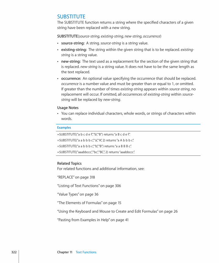
SUBSTITUTEThe SUBSTITUTE function returns a string where the specified characters of a given string have been replaced with a new string.
SUBSTITUTE(source-string, existing-string, new-string, occurrence)
 source-string:� A string. source-string is a string value.
 existing-string:� The string within the given string that is to be replaced. existing-string is a string value.
 new-string:� The text used as a replacement for the section of the given string that is replaced. new-string is a string value. It does not have to be the same length as the text replaced.
 occurrence:� An optional value specifying the occurrence that should be replaced. occurrence is a number value and must be greater than or equal to 1, or omitted. If greater than the number of times existing-string appears within source-string, no replacement will occur. If omitted, all occurrences of existing-string within source-string will be replaced by new-string.
Usage NotesYou can replace individual characters, whole words, or strings of characters within Âwords.
Examples
=SUBSTITUTE(”a b c d e f”, “b”, “B”) returns “a B c d e f”.
=SUBSTITUTE(”a a b b b c”, “a”, “A”, 2) returns “a A b b b c”.
=SUBSTITUTE(”a a b b b c”, “b”, “B”) returns “a a B B B c”.
=SUBSTITUTE(”aaabbccc”, “bc”, “BC”, 2) returns “aaabbccc”.
Related TopicsFor related functions and additional information, see:
“REPLACE” on page 318
“Listing of Text Functions” on page 306
“Value Types” on page 36
“The Elements of Formulas” on page 15
“Using the Keyboard and Mouse to Create and Edit Formulas” on page 26
“Pasting from Examples in Help” on page 41
322 Chapter 11 Text Functions

Chapter 11 Text Functions 323
TThe T function returns the text contained in a cell. This function is included for compatibility with tables imported from other spreadsheet applications.
T(cell)
 cell:� A reference to a single table cell. cell is a reference value to a single cell that can contain any value, or be empty.
Usage NotesIf the cell doesn’t contain a string, T returns an empty string. Â
Examples
If cell A1 contains “text” and cell B1 is empty:
=T(A1) returns “text”
=T(B1) returns nothing.
Related TopicsFor related functions and additional information, see:
“Listing of Text Functions” on page 306
“Value Types” on page 36
“The Elements of Formulas” on page 15
“Using the Keyboard and Mouse to Create and Edit Formulas” on page 26
“Pasting from Examples in Help” on page 41
TRIMThe TRIM function returns a string based on a given string, after removing extra spaces.
TRIM(source-string)
 source-string:� A string. source-string is a string value.
Usage NotesTRIM removes all spaces before the first character, all spaces after the last character, Âand all duplicate spaces between characters, leaving only single spaces between words.
Example
=TRIM(” spaces spaces spaces “) returns “spaces spaces spaces” (the leading and trailing space were removed).

Related TopicsFor related functions and additional information, see:
“Listing of Text Functions” on page 306
“Value Types” on page 36
“The Elements of Formulas” on page 15
“Using the Keyboard and Mouse to Create and Edit Formulas” on page 26
“Pasting from Examples in Help” on page 41
UPPERThe UPPER function returns a string that is entirely uppercase, regardless of the case of the characters in the specified string.
UPPER(source-string)
 source-string:� A string. source-string is a string value.
Examples
=UPPER(”a b c”) returns “A B C”.
=UPPER(”First”) returns “FIRST”.
Related TopicsFor related functions and additional information, see:
“LOWER” on page 316
“PROPER” on page 317
“Listing of Text Functions” on page 306
“Value Types” on page 36
“The Elements of Formulas” on page 15
“Using the Keyboard and Mouse to Create and Edit Formulas” on page 26
“Pasting from Examples in Help” on page 41
324 Chapter 11 Text Functions

Chapter 11 Text Functions 325
VALUEThe VALUE function returns a number value even if the argument is formatted as text. This function is included for compatibility with tables imported from other spreadsheet applications.
VALUE(source-string)
 source-string:� A string. source-string is a string value.
Usage NotesYou’ll never need to use the VALUE function in a new table, as numbers in text are Âautomatically converted for you.
Only the formatted text is converted. For example, if the string $100.001 is typed into Âa cell, the default format will display only two decimals ($100.00). If VALUE refers to this cell, it will return 100, the value of the formatted text, not 100.001.
If the argument can’t be returned as a number value (does not contain a number), Âthe function returns an error.
Examples
=VALUE(”22”) returns the number 22.
=VALUE(RIGHT(”The year 1953”, 2)) returns the number 53.
Related TopicsFor related functions and additional information, see:
“Listing of Text Functions” on page 306
“Value Types” on page 36
“The Elements of Formulas” on page 15
“Using the Keyboard and Mouse to Create and Edit Formulas” on page 26
“Pasting from Examples in Help” on page 41

326
The trigonometric functions help you work with angles and their components.
Listing of Trigonometric FunctionsiWork provides these trigonometric functions for use with tables.
Function Description
“ACOS” (page 327) The ACOS function returns the inverse cosine (arccosine) of a number.
“ACOSH” (page 328) The ACOSH function returns the inverse hyperbolic cosine (hyperbolic arccosine) of a number.
“ASIN” (page 329) The ASIN function returns the arcsine (the inverse sine) of a number.
“ASINH” (page 329) The ASINH function returns the inverse hyperbolic sine of a number.
“ATAN” (page 330) The ATAN function returns the inverse tangent (arctangent) of a number.
“ATAN2” (page 331) The ATAN2 function returns the angle, relative to the positive x-axis, of the line passing through the origin and the specified point.
“ATANH” (page 332) The ATANH function returns the inverse hyperbolic tangent of a number.
“COS” (page 333) The COS function returns the cosine of an angle that is expressed in radians.
“COSH” (page 334) The COSH function returns the hyperbolic cosine of a number.
12Trigonometric Functions

Chapter 12 Trigonometric Functions 327
Function Description
“DEGREES” (page 334) The DEGREES function returns the number of degrees in an angle expressed in radians.
“RADIANS” (page 335) The RADIANS function returns the number of radians in an angle expressed in degrees.
“SIN” (page 336) The SIN function returns the sine of an angle that is expressed in radians.
“SINH” (page 337) The SINH function returns the hyperbolic sine of the specified number.
“TAN” (page 338) The TAN function returns the tangent of an angle that is expressed in radians.
“TANH” (page 339) The TANH function returns the hyperbolic tangent of the specified number.
ACOSThe ACOS function returns the inverse cosine (arccosine) of a number.
ACOS(num)
 num:� A number. num is a number value in the range –1 to 1.
Usage NotesThe ACOS function takes a cosine value and returns a corresponding angle. The Âresulting angle is expressed in radians, in the range 0 to π (pi). To see the resulting angle in degrees instead of radians, wrap this function in the DEGREES function; that is, =DEGREES(ACOS(num)).
Examples
=ACOS(SQRT(2)/2) returns 0.785398163397448, which is approximately π/4.
=ACOS(0.54030230586814) returns 1.
=DEGREES(ACOS(.5)) returns 60, the degree measure of an angle that has a cosine of 0.5.
Related TopicsFor related functions and additional information, see:
“ACOSH” on page 328
“COS” on page 333
“COSH” on page 334
“DEGREES” on page 334
“Listing of Trigonometric Functions” on page 326

“Value Types” on page 36
“The Elements of Formulas” on page 15
“Using the Keyboard and Mouse to Create and Edit Formulas” on page 26
“Pasting from Examples in Help” on page 41
ACOSHThe ACOSH function returns the inverse hyperbolic cosine (hyperbolic arccosine) of a number.
ACOSH(num)
 num:� A number. num is a number value that must be greater than or equal to 1.
Examples
=ACOSH(10.0676619957778) returns 3.
=ACOSH(COSH(5)) returns 5.
Related TopicsFor related functions and additional information, see:
“ACOS” on page 327
“COS” on page 333
“COSH” on page 334
“Listing of Trigonometric Functions” on page 326
“Value Types” on page 36
“The Elements of Formulas” on page 15
“Using the Keyboard and Mouse to Create and Edit Formulas” on page 26
“Pasting from Examples in Help” on page 41
328 Chapter 12 Trigonometric Functions

Chapter 12 Trigonometric Functions 329
ASINThe ASIN function returns the arcsine (the inverse sine) of a number.
ASIN(num)
 num:� A number. num is a number value that must be greater than or equal to 1.
Usage NotesThe ASIN function takes a sine and returns the corresponding angle. The result Âis expressed in radians, in the range –pi/2 to +pi/2. To see the resulting angle in degrees instead of radians, wrap this function in the DEGREES function; that is, =DEGREES(ASIN(num)).
Examples
=ASIN(0.841470985) returns 1, the radian measure (approximately 57.3 degrees) of the angle that has a sine of 0.8411470984807897.
=DEGREES(ASIN(0.5)) returns 30, the degree measure of the angle that has a sine of 0.5.
Related TopicsFor related functions and additional information, see:
“ASINH” on page 329
“DEGREES” on page 334
“SIN” on page 336
“SINH” on page 337
“Listing of Trigonometric Functions” on page 326
“Value Types” on page 36
“The Elements of Formulas” on page 15
“Using the Keyboard and Mouse to Create and Edit Formulas” on page 26
“Pasting from Examples in Help” on page 41
ASINHThe ASINH function returns the inverse hyperbolic sine of a number.
ASINH(num)
 num:� A number. num is a number value.

Examples
=ASINH(27.2899171971277) returns 4.
=ASINH(SINH(1)) returns 1.
Related TopicsFor related functions and additional information, see:
“ASIN” on page 329
“SIN” on page 336
“SINH” on page 337
“Listing of Trigonometric Functions” on page 326
“Value Types” on page 36
“The Elements of Formulas” on page 15
“Using the Keyboard and Mouse to Create and Edit Formulas” on page 26
“Pasting from Examples in Help” on page 41
ATANThe ATAN function returns the inverse tangent (arctangent) of a number.
ATAN(num)
 num:� A number. num is a number value.
Usage NotesThe ATAN function takes a tangent and returns the corresponding angle, Âexpressed in radians in the range –pi/2 to +pi/2. To see the resulting angle in degrees instead of radians, wrap this function in the DEGREES function; that is, =DEGREES(ATAN(num)).
Examples
=ATAN(1) returns the angle measure 0.785398163 radians (45 degrees), which has a tangent of 1.
=DEGREES(ATAN(1)) returns 45.
Related TopicsFor related functions and additional information, see:
“ATAN2” on page 331
“ATANH” on page 332
330 Chapter 12 Trigonometric Functions

Chapter 12 Trigonometric Functions 331
“DEGREES” on page 334
“TAN” on page 338
“TANH” on page 339
“Listing of Trigonometric Functions” on page 326
“Value Types” on page 36
“The Elements of Formulas” on page 15
“Using the Keyboard and Mouse to Create and Edit Formulas” on page 26
“Pasting from Examples in Help” on page 41
ATAN2The ATAN2 function returns the angle, relative to the positive x-axis, of the line passing through the origin and the specified point.
ATAN2(x-point, y-point)
 x-point:� The x-coordinate of the point the line passes through. x-point is a number value.
 y-point:� The y-coordinate of the point the line passes through. y-point is a number value.
Usage NotesThe angle is expressed in radians, in the range –pi through +pi. To see the resulting Âangle in degrees instead of radians, wrap this function in the DEGREES function; that is, =DEGREES(ATAN2(x-point, y-point)).
Examples
=ATAN2(1, 1) returns 0.78539816 radians (45 degrees), the angle of a line segment from the origin to point (1, 1).
=DEGREES(ATAN2(5, 5)) returns 45.
Related TopicsFor related functions and additional information, see:
“ATAN” on page 330
“ATANH” on page 332
“DEGREES” on page 334
“TAN” on page 338

“TANH” on page 339
“Listing of Trigonometric Functions” on page 326
“Value Types” on page 36
“The Elements of Formulas” on page 15
“Using the Keyboard and Mouse to Create and Edit Formulas” on page 26
“Pasting from Examples in Help” on page 41
ATANHThe ATANH function returns the inverse hyperbolic tangent of a number.
ATANH(num)
 num:� A number. num is a number value that must be greater than –1 and less than 1.
Examples
=ATANH(0.995054753686731) returns 3.
=ATANH(TANH(2)) returns 2.
Related TopicsFor related functions and additional information, see:
“ATAN” on page 330
“ATAN2” on page 331
“TAN” on page 338
“TANH” on page 339
“Listing of Trigonometric Functions” on page 326
“Value Types” on page 36
“The Elements of Formulas” on page 15
“Using the Keyboard and Mouse to Create and Edit Formulas” on page 26
“Pasting from Examples in Help” on page 41
332 Chapter 12 Trigonometric Functions

Chapter 12 Trigonometric Functions 333
COSThe COS function returns the cosine of an angle that is expressed in radians.
COS(radian-angle)
 radian-angle:� An angle, expressed in radians. radian-angle is a number value. Although it can be any value, it would normally be in the range –π to +π (–pi to +pi).
Usage NotesTo return an angle in degrees, use the DEGREES function (to convert radians to Âdegrees) with this function; that is, =DEGREES(COS(radian-angle)).
Examples
=COS(1) returns 0.540302306, the cosine of 1 radian (approximately 57.3 degrees).
=COS(RADIANS(60)) returns 0.5, the cosine of 60 degrees.
=COS(PI()/3) returns 0.5, π/3 radians (60 degrees).
=COS(PI()) returns –1, the cosine of π radians (180 degrees).
Related TopicsFor related functions and additional information, see:
“ACOS” on page 327
“ACOSH” on page 328
“COSH” on page 334
“DEGREES” on page 334
“SIN” on page 336
“TAN” on page 338
“Listing of Trigonometric Functions” on page 326
“Value Types” on page 36
“The Elements of Formulas” on page 15
“Using the Keyboard and Mouse to Create and Edit Formulas” on page 26
“Pasting from Examples in Help” on page 41

COSHThe COSH function returns the hyperbolic cosine of a number.
COSH(num)
 num:� A number. num is a number value.
Examples
=COSH(0) returns 1.
=COSH(1) returns 1.543.
=COSH(5) returns 74.21.
=COSH(10) returns 11,013.233.
Related TopicsFor related functions and additional information, see:
“ACOS” on page 327
“ACOSH” on page 328
“COS” on page 333
“Listing of Trigonometric Functions” on page 326
“Value Types” on page 36
“The Elements of Formulas” on page 15
“Using the Keyboard and Mouse to Create and Edit Formulas” on page 26
“Pasting from Examples in Help” on page 41
DEGREESThe DEGREES function returns the number of degrees in an angle expressed in radians.
DEGREES(radian-angle)
 radian-angle:� An angle, expressed in radians. radian-angle is a number value. Although it can be any value, it would normally be in the range –2π to 2π (–2 pi to +2 pi).
Examples
=DEGREES(PI()) returns 180 (π radians = 180 degrees).
=DEGREES(1) returns 57.2957795130823, which is approximately the number of degrees per radian.
334 Chapter 12 Trigonometric Functions

Chapter 12 Trigonometric Functions 335
Related TopicsFor related functions and additional information, see:
“ACOS” on page 327
“ASIN” on page 329
“ATAN” on page 330
“ATAN2” on page 331
“COS” on page 333
“SIN” on page 336
“TAN” on page 338
“Listing of Trigonometric Functions” on page 326
“Value Types” on page 36
“The Elements of Formulas” on page 15
“Using the Keyboard and Mouse to Create and Edit Formulas” on page 26
“Pasting from Examples in Help” on page 41
RADIANSThe RADIANS function returns the number of radians in an angle expressed in degrees.
RADIANS(degree-angle)
 degree-angle:� An angle, expressed in degrees. degree-angle is a number value. Although it can be any value, it would normally be in the range –360 to +360.
Usage NotesThis function is useful if you wish to use an angle expressed in degrees with Âany of the standard geometric functions, as they expect an angle expressed in radians. Wrap the argument, expressed in degrees, in this function; for example, =COS(RADIANS(degree-angle).
Examples
=RADIANS(90) returns 1.5708 (90 degrees is approximately 1.5708 radians).
=RADIANS(57.2957795130823) returns 1 (1 radian is approximately 57.296 degrees).
Related TopicsFor related functions and additional information, see:

“ACOS” on page 327
“ASIN” on page 329
“ATAN” on page 330
“ATAN2” on page 331
“COS” on page 333
“SIN” on page 336
“TAN” on page 338
“Listing of Trigonometric Functions” on page 326
“Value Types” on page 36
“The Elements of Formulas” on page 15
“Using the Keyboard and Mouse to Create and Edit Formulas” on page 26
“Pasting from Examples in Help” on page 41
SINThe SIN function returns the sine of an angle that is expressed in radians.
SIN(radian-angle)
 radian-angle:� An angle, expressed in radians. radian-angle is a number value. Although it can be any value, it would normally be in the range –π to π (–pi to +pi).
Usage NotesTo return an angle in degrees, use the DEGREES function (to convert radians to Âdegrees) with this function; that is, =DEGREES(SIN(radian-angle)).
Examples
=SIN(1) returns 0.841470985, the sine of 1 radian (approximately 57.3 degrees).
=SIN(RADIANS(30)) returns 0.5, the sine of 30 degrees.
=SIN(PI()/2) returns 1, the sine of π/2 radians (90 degrees).
Related TopicsFor related functions and additional information, see:
“ASIN” on page 329
“ASINH” on page 329
336 Chapter 12 Trigonometric Functions

Chapter 12 Trigonometric Functions 337
“COS” on page 333
“DEGREES” on page 334
“SINH” on page 337
“TAN” on page 338
“Listing of Trigonometric Functions” on page 326
“Value Types” on page 36
“The Elements of Formulas” on page 15
“Using the Keyboard and Mouse to Create and Edit Formulas” on page 26
“Pasting from Examples in Help” on page 41
SINHThe SINH function returns the hyperbolic sine of the specified number.
SINH(num)
 num:� A number. num is a number value.
Examples
=SINH(0) returns 0.
=SINH(1) returns 1.175.
=SINH(5) returns 74.203.
=SINH(10) returns 11013.233.
Related TopicsFor related functions and additional information, see:
“ASIN” on page 329
“ASINH” on page 329
“SIN” on page 336
“Listing of Trigonometric Functions” on page 326
“Value Types” on page 36
“The Elements of Formulas” on page 15
“Using the Keyboard and Mouse to Create and Edit Formulas” on page 26
“Pasting from Examples in Help” on page 41

TANThe TAN function returns the tangent of an angle that is expressed in radians.
TAN(radian-angle)
 radian-angle:� An angle, expressed in radians. radian-angle is a number value. Although it can be any value, it would normally be in the range –pi to +pi.
Usage NotesThe tangent is the ratio of the sine to the cosine. Â
To return an angle in degrees, use the DEGREES function (to convert radians to Âdegrees) with this function; that is, =DEGREES(TAN(radian-angle)).
Examples
=TAN(1) returns 1.557407725, the tangent of 1 radian (approximately 57.3 degrees).
=TAN(RADIANS(45)) returns 1, the tangent of a 45-degree angle.
=TAN(3*PI()/4) returns -1.
Related TopicsFor related functions and additional information, see:
“ATAN” on page 330
“ATAN2” on page 331
“ATANH” on page 332
“COS” on page 333
“DEGREES” on page 334
“SIN” on page 336
“TANH” on page 339
“Listing of Trigonometric Functions” on page 326
“Value Types” on page 36
“The Elements of Formulas” on page 15
“Using the Keyboard and Mouse to Create and Edit Formulas” on page 26
“Pasting from Examples in Help” on page 41
338 Chapter 12 Trigonometric Functions

Chapter 12 Trigonometric Functions 339
TANHThe TANH function returns the hyperbolic tangent of the specified number.
TANH(num)
 num:� A number. num is a number value.
Examples
=TANH(0) returns 0.
=TANH(1) returns 0.762.
=TANH(5) returns 0.999909.
=TANH(10) returns 0.999999996.
Related TopicsFor related functions and additional information, see:
“ATAN” on page 330
“ATAN2” on page 331
“ATANH” on page 332
“TAN” on page 338
“Listing of Trigonometric Functions” on page 326
“Value Types” on page 36
“The Elements of Formulas” on page 15
“Using the Keyboard and Mouse to Create and Edit Formulas” on page 26
“Pasting from Examples in Help” on page 41

340
The in-depth examples and additional topics in this chapter illustrate working with some of the more complex functions.
Additional Examples and Topics IncludedThe following table tells you where to find in-depth examples and additional topics that illustrate working with some of the more complex functions with real-world examples.
If you wish to see an example or learn more about
See this section
The definitions and specification of arguments used in financial functions
“Common Arguments Used in Financial Functions” on page 341
The time value of money (TVM) functions “Choosing Which Time Value of Money Function to Use” on page 348
TVM functions dealing with fixed periodic cash flows and fixed interest rates
“Regular Cash Flows and Time Intervals” on page 348
TVM functions that can deal with uneven (variable periodic) cash flows
“Irregular Cash Flows and Time Intervals” on page 350
The function that may be most helpful in answering a common financial question
“Which Function Should You Use to Solve Common Financial Questions?” on page 351
Using financial functions to create a loan amortization table
“Example of a Loan Amortization Table” on page 353
The various functions that round numbers “More on Rounding” on page 355
Using logical and information functions together to build a more powerful formula
“Using Logical and Information Functions Together” on page 358
Understanding conditions and how to use wildcards with conditions
“Specifying Conditions and Using Wildcards” on page 360
Using statistical functions to analyze the results of a survey
“Survey Results Example” on page 362
13Additional Examples and Topics

Chapter 13 Additional Examples and Topics 341
Common Arguments Used in Financial FunctionsMany arguments are common among related financial functions. This section provides information regarding these arguments. Date arguments (issue, maturity, and settle) are not included. Arguments that are used by only a single financial function are also not included.
annual-rateBonds and other fixed-rate, interest-bearing debt securities have a stated coupon or annual interest rate used to determine periodic interest payments. annual-rate is used to represent the annual interest rate, whether it is called a coupon rate or an annual interest rate.
coupon-rate is specified as a decimal number representing the annual coupon rate. In some functions, coupon-rate can be 0 (if the security does not pay periodic interest), but coupon-rate cannot be negative.
Assume that you own a security with a face value of $1,000,000 and that pays annual interest of 4.5% based on the face value. coupon-rate would be 0.045. frequency of payment does not matter.
annual-yieldBonds and other interest-bearing and discount debt securities have a yield that is calculated using the coupon interest rate and the current price of the bond.
annual-yield is specified as a decimal number representing the security’s annual yield, which is commonly stated as a percentage. annual-yield must be greater than 0.
Assume that you are considering the purchase of a particular bond. As the price of a bond goes down, its yield goes up. Conversely, if the price of the bond rises, its yield decreases. Your broker checks the pricing screens and tells you that the bond you are considering has a coupon rate of 3.25% and an annual yield of 4.5%, based on its current price (the bond is trading at a discount). annual-yield would be 0.045.
cash-flowAnnuities, loans, and investments have cash flows. One cash flow is the initial amount paid or received, if any. Other cash flows are other receipts or payments at a specific point in time.
cash-flow is specified as a number, usually formatted as currency. Amounts received are specified as positive numbers and amounts paid are specified as negative numbers.
Assume that there is a townhouse that you plan to purchase, rent out for a period of time, and then resell. The initial cash purchase payment (which might consist of a down payment and closing costs), loan payments, repairs and maintenance, advertising, and similar costs, would be payments (negative cash flows). Rents received from tenants, tax benefits received through a reduction of other taxes, and the amount received upon sale would be receipts (positive cash flows).
costThe initial cost of the asset to be depreciated is generally the purchase price, including taxes, delivery, and setup. Certain tax benefits may be deducted from the cost.
cost is specified as number, usually formatted as currency. cost must be greater than 0.
Assume that you purchase a new digital photocopy machine for your office. The purchase price of the photocopy machine was $2,625 with tax. The vendor charged $100 to deliver and set it up. The photocopy machine is expected to be used for 4 years, at which time it is expected to have a resale value of $400. cost would be $2,725.
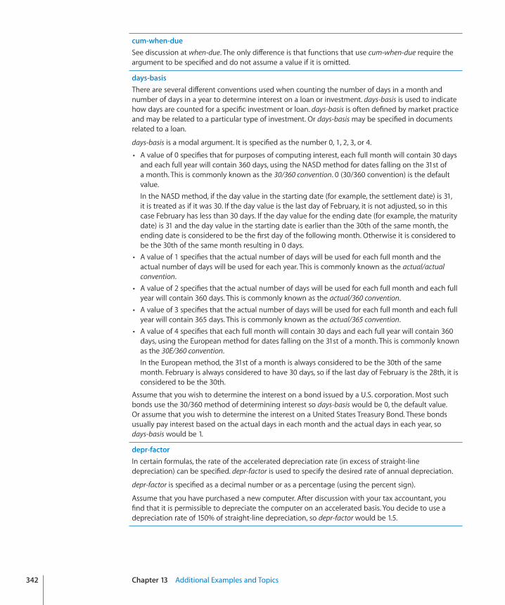
cum-when-dueSee discussion at when-due. The only difference is that functions that use cum-when-due require the argument to be specified and do not assume a value if it is omitted.
days-basisThere are several different conventions used when counting the number of days in a month and number of days in a year to determine interest on a loan or investment. days-basis is used to indicate how days are counted for a specific investment or loan. days-basis is often defined by market practice and may be related to a particular type of investment. Or days-basis may be specified in documents related to a loan.
days-basis is a modal argument. It is specified as the number 0, 1, 2, 3, or 4.
 A value of 0 specifies that for purposes of computing interest, each full month will contain 30 days and each full year will contain 360 days, using the NASD method for dates falling on the 31st of a month. This is commonly known as the 30/360 convention. 0 (30/360 convention) is the default value.In the NASD method, if the day value in the starting date (for example, the settlement date) is 31, it is treated as if it was 30. If the day value is the last day of February, it is not adjusted, so in this case February has less than 30 days. If the day value for the ending date (for example, the maturity date) is 31 and the day value in the starting date is earlier than the 30th of the same month, the ending date is considered to be the first day of the following month. Otherwise it is considered to be the 30th of the same month resulting in 0 days.
 A value of 1 specifies that the actual number of days will be used for each full month and the actual number of days will be used for each year. This is commonly known as the actual/actual convention.
 A value of 2 specifies that the actual number of days will be used for each full month and each full year will contain 360 days. This is commonly known as the actual/360 convention.
 A value of 3 specifies that the actual number of days will be used for each full month and each full year will contain 365 days. This is commonly known as the actual/365 convention.
 A value of 4 specifies that each full month will contain 30 days and each full year will contain 360 days, using the European method for dates falling on the 31st of a month. This is commonly known as the 30E/360 convention.In the European method, the 31st of a month is always considered to be the 30th of the same month. February is always considered to have 30 days, so if the last day of February is the 28th, it is considered to be the 30th.
Assume that you wish to determine the interest on a bond issued by a U.S. corporation. Most such bonds use the 30/360 method of determining interest so days-basis would be 0, the default value. Or assume that you wish to determine the interest on a United States Treasury Bond. These bonds usually pay interest based on the actual days in each month and the actual days in each year, so days-basis would be 1.
depr-factorIn certain formulas, the rate of the accelerated depreciation rate (in excess of straight-line depreciation) can be specified. depr-factor is used to specify the desired rate of annual depreciation.
depr-factor is specified as a decimal number or as a percentage (using the percent sign).
Assume that you have purchased a new computer. After discussion with your tax accountant, you find that it is permissible to depreciate the computer on an accelerated basis. You decide to use a depreciation rate of 150% of straight-line depreciation, so depr-factor would be 1.5.
342 Chapter 13 Additional Examples and Topics

Chapter 13 Additional Examples and Topics 343
depr-periodCertain functions return the amount of depreciation for a specified period. depr-period is used to specify the period.
depr-period is specified as a number representing the desired depreciation period using the same time frame (for example, monthly, quarterly, or annually) as life.
Assume that you purchase a new digital photocopy machine for your office. The purchase price of the photocopy machine was $2,625 with tax. The vendor charged $100 to deliver and set it up. The photocopy machine is expected to be used for 4 years, at which time it is expected to have a resale value of $400. If you wished to determine the depreciation for the third year, depr-period would be 3.
effective-int-rateAnnuities and investments have an effective interest rate, which is calculated using the nominal (stated or coupon) rate and the number of interest payments per year.
effective-int-rate is specified as a decimal number and must be greater than 0.
Assume that you own a security with a face value of $1,000,000 that pays annual interest of 4.5% based on the face value, on a quarterly basis, which is an effective rate of approximately 4.58%. effective-int-rate would be 0.0458. See also the description of nominal-rate and num-periods-year.
end-perCertain functions return principal or interest for a series of specified payments. end-per is used to indicate the last payment to be included in the value returned. See also the discussion of start-per.
end-per is specified as a number and must be greater than 0.
Assume that you are purchasing a home. The mortgage broker offers you a loan with an initial balance of $200,000, a term of 10 years, an annual interest rate of 6.0%, fixed monthly payments of $1070.45, and a balance to be refinanced at maturity of $100,000. If you wished to know the total amount of interest paid in the third year, start-per would be 25 and end-per would be 36.
estimateAn estimate of the expected outcome is used by some financial functions.
estimate is specified as a decimal number. For example, 13% is specified as 0.13. estimate can be negative, if a loss is expected. If estimate is not specified, 0.10 is used as the default value.
If you do not have an idea as to the expected outcome and the default value does not result in a solution, initially try a larger positive estimate. If this does not result in an outcome, try a small negative estimate.
frequencyAn investment may pay interest on a periodic basis. frequency is used to indicate how often interest is paid.
frequency is the number 1, 2, or 4.
 A value of 1 indicates that the investment pays interest annually (once a year).  A value of 2 indicates that the investment pays interest semiannually (twice per year).  A value of 4 indicates that the investment pays interest quarterly (four times per year).
Assume that you are evaluating a corporate bond that pays interest quarterly. frequency would be 4. Or assume you are evaluating a government bond that pays interest semiannually. frequency would be 2.

future-valueA future value is a cash flow received or paid at the end of the investment or loan period or the cash value remaining after the final payment.
future-value is specified as a number, usually formatted as currency. Since future-value is a cash flow, amounts received are specified as positive numbers and amounts paid are specified as negative numbers.
Assume that there is a townhouse that you plan to purchase, rent out for a period of time, and then resell. The estimated future sales price could be a future-value and would be positive. Or assume that you lease a car and that the lease contains a provision allowing you to buy the car for a specified price at the end of the lease term. The amount of that payment could be a future-value and would be negative. Or assume that you have a mortgage loan that at the end of 10 years has a balloon payment due. The balloon payment could be a future-value and would be negative.
invest-amountThe initial amount invested in a bond is specified using invest-amount.
invest-amount is specified as a number, usually formatted as currency. invest-amount must be greater than 0.
Assume that you purchase a bond for $800. invest-amount would be $800.
lifeAssets are depreciated over a specific period, known as the depreciable life or the expected useful life. Generally for accounting purposes the expected useful life of the asset would be used for depreciation, whereas for other purposes (such as preparing a tax return) the depreciable life may be specified by regulation or practice.
life is specified as a number. life must be greater than 0.
Assume that you purchase a new digital photocopy machine for your office. The purchase price of the photocopy machine was $2,625 with tax. The vendor charged $100 to deliver and set it up. The photocopy machine is expected to be used for 4 years, at which time it is expected to have a resale value of $400. life is 4.
nominal-rateAnnuities and investments have a nominal interest rate, which is calculated using the effective interest rate and the number of compounding periods per year.
nominal-rate is specified as a decimal number and must be greater than 0.
Assume that own a security with a face value of $1,000,000 that pays annual interest of 4.5% based on the face value, on a quarterly basis, which is an effective rate of approximately 4.58%. nominal-rate would be 0.045. See also the description of effective-int-rate and num-periods-year.
num-periodsThe number of periods (num-periods) is the total periods of a repeating cash flow, or the length of a loan, or the length of the investment period.
num-periods is specified as a number using the same time frame (for example, monthly, quarterly, or annually) as related arguments used by the function.
Assume that you are purchasing a home. The mortgage broker offers you a loan with an initial balance of $200,000, a term of 10 years, an annual interest rate of 6.0%, fixed monthly payments, and a balance to be refinanced at maturity of $100,000. num-periods would be 120 (12 monthly payments for 10 years). Or assume that you invest your savings in a certificate of deposit that has a term of 5 years and compounds interest quarterly. num-periods would be 20 (4 quarterly compounding periods for 5 years).
344 Chapter 13 Additional Examples and Topics

Chapter 13 Additional Examples and Topics 345
num-periods-yearThe calculation of the effective and nominal interest rates is based on the number of interest compounding periods per year. num-periods-year is used to specify the number of periods.
num-periods-year is specified as a number and must be greater than 0.
Assume that you have purchased a certificate of deposit that pays interest annually, compounded quarterly. If you wanted to determine the effective interest rate, num-periods-year would be 4. See also the description of effective-int-rate and nominal-rate.
parThe par value of a security is generally its face or maturity value.
par is specified as a number, usually formatted as currency.
par is often a number like 100, 1,000, or 1,000,000.
Assume that you are considering purchasing a corporate bond. The prospectus for the bond states that each bond will be issued with a face and maturity value of $1,000. The $1,000 would be the par value of the bond.
paymentA payment is a fixed, periodic cash flow received or paid over an investment or loan period.
payment is specified as a number, usually formatted as currency. Since payment is a cash flow, amounts received are specified as positive numbers and amounts paid are specified as negative numbers.
payment often includes both principal and interest elements, but does not usually include other amounts.
Assume that there is a townhouse that you plan to purchase, rent out for a period of time, and then resell. The amount of the monthly mortgage payment could be a payment and would be negative. The rent payment received each month could also be a payment and would be positive.
periodCertain functions return a principal or interest value for a given period. period is used to indicate the desired period.
period is specified as a number and must be greater than 0.
Assume that you are purchasing a home. The mortgage broker offers you a loan with an initial balance of $200,000, a term of 10 years, an annual interest rate of 6.0%, fixed monthly payments of $1070.45, and a balance to be refinanced at maturity of $100,000. If you wished to know the amount of interest in the first payment of the third year, period would be 25, since payments are monthly.
periodic-discount-rateThe discount rate is the interest rate representing the desired yield used to value (or discount) a series of cash flows.
periodic-discount-rate is specified as a decimal (for example, 0.08) or delimited with a percent sign (for example, 8%). It is specified using the same time frame as the time frame used for the cash flows. For example, if the cash flows are monthly and the desired annual discount rate is 8%, periodic-discount-rate must be specified as 0.00667 or 0.667% (0.08 divided by 12).
Assume that you are evaluating the possible purchase of a business. As part of your evaluation, you determine the expected monthly cash flows from the business along with the requested purchase price and estimated future resale price. You decide, based on alternative investment opportunities and risk, that you will not invest unless the net cash flows yield at least an 18% annual interest rate. periodic-discount-rate would be 0.015 (0.18 / 12 as specified cash flows are monthly).

periodic-rateIn some cases, when working with a series of cash flows, or an investment, or a loan, it may be necessary to know the interest rate each period. This is the periodic-rate.
periodic-rate is specified as a decimal number using the same time frame (for example, monthly, quarterly, or annually) as other arguments (num-periods or payment).
Assume that you are purchasing a home. The mortgage broker offers you a loan with an initial balance of $200,000, a term of 10 years, an annual interest rate of 6.0%, fixed monthly payments, and a balance to be refinanced at maturity of $100,000. periodic-rate would be 0.005 (annual rate divided by 12 to match up with the monthly payment). Or assume that you invest your savings in a certificate of deposit that has a term of 5 years, has a nominal annual interest rate of 4.5%, and interest compounds quarterly. periodic-rate would be 0.0125 (annual rate divided by 4 to match the quarterly compounding periods).
present-valueA present value is a cash flow received or paid at the beginning of the investment or loan period.
present-value is specified as a number, usually formatted as currency. Since present-value is a cash flow, amounts received are specified as positive numbers and amounts paid are specified as negative numbers.
Assume that there is a townhouse that you plan to purchase, rent out for a period of time, and then resell. The initial cash purchase payment (which might consist of a down payment and closing costs) could be a present-value and would be negative. The initial principal amount of a loan on the townhouse could also be a present-value and would be positive.
priceThe purchase price is the amount paid to buy a bond or other interest-bearing or discount debt security. The purchase price does not include accrued interest purchased with the security.
price is specified as a number representing the amount paid per $100 of face value (purchase price / face value * 100). price must be greater than 0.
Assume that you own a security that has a face value of $1,000,000. If you paid $965,000 when you purchased the security, excluding accrued interest if any, price would be 96.50 ($965,000 / $1,000,000 * 100).
redemptionBonds and other interest-bearing and discount debt securities usually have a stated redemption value. This is the amount that will be received when the debt security matures.
redemption is specified as a number representing the amount that will be received per $100 of face value (redemption value / face value * 100). Often, redemption is 100, meaning that the security’s redemption value is equal to its face value. value must be greater than 0.
Assume that you own a security that has a face value of $1,000,000 and for which you will receive $1,000,000 at maturity. redemption would be 100 ($1,000,000 / $1,000,000 * 100), because the face value and the redemption value are the same, a common case. Assume further though that the issuer of this security offers to redeem the security before maturity and has offered $1,025,000 if redeemed one year early. redemption would be 102.50 ($1,025,000 / $1,000,000 * 100).
346 Chapter 13 Additional Examples and Topics

Chapter 13 Additional Examples and Topics 347
salvageAssets often have value remaining at the end of the depreciable life or the expected useful life. This is the salvage value.
salvage is specified as a number, usually formatted as currency. salvage can be 0, but cannot be negative.
Assume that you purchase a new digital photocopy machine for your office. The purchase price of the photocopy machine was $2,625 with tax. The vendor charged $100 to deliver and set it up. The photocopy machine is expected to be used for 4 years, at which time it is expected to have a resale value of $400. salvage is $400.
start-perCertain functions return principal or interest for a series of specified payments. start-per is used to indicate the first payment to be included in the value returned. See also the discussion of end-per.
start-per is specified as a number and must be greater than 0.
Assume that you are purchasing a home. The mortgage broker offers you a loan with an initial balance of $200,000, a term of 10 years, an annual interest rate of 6.0%, fixed monthly payments of $1070.45, and a balance to be refinanced at maturity of $100,000. If you wished to know the total amount of interest paid in the third year, start-per would be 25 and end-per would be 36.
when-duePayments can be generalized to occur at the beginning or end of a period. when-due is used to indicate whether a payment occurs at the beginning or end of a period.
when-due is a modal argument. It can be the number 0 or 1.
 A value of 0 specifies that the payment is treated as being received or made at the end of each period. 0 is the default value.
 A value of 1 specifies that the payment is treated as being received or made at the beginning of each period.
Assume that you are purchasing a home. The mortgage broker offers you a loan with an initial balance of $200,000, a term of 10 years, an annual interest rate of 6.0%, fixed monthly payments, and a balance to be refinanced at maturity of $100,000. when-due would be 0 (the default) since payments are made at the end of each month. Or assume you own an apartment that you rent and that you require the tenant to pay rent on the first of each month. when-due would be 1, since this payment is being made by the tenant at the beginning of the monthly period.

Choosing Which Time Value of Money Function to UseThis section provides additional information regarding the functions used to solve time value of money problems. Time value of money, or TVM, problems involve cash flows over time and interest rates. This section contains several parts.
“Regular Cash Flows and Time Intervals” on page 348 discusses the TVM functions used with regular cash flows, regular time intervals, and fixed interest rates.
“Irregular Cash Flows and Time Intervals” on page 350 discusses the TVM functions used with irregular cash flows, irregular time intervals, or both.
“Which Function Should You Use to Solve Common Financial Questions?” on page 351 describes several common TVM problems (such as which function would be used to compute interest on a savings account) along with the functions that might be used in solving the problem.
Regular Cash Flows and Time IntervalsThe primary functions used with regular periodic cash flows (payments of a constant amount and all cash flows at constant intervals) and fixed interest rates are interrelated.
Function and its purpose Arguments used by the function
“FV” (page 120) is the function to use if you wish to determine what the future value (what it is worth at a future point in time) of a series of cash flows will be, considering the other factors such as the interest rate. It solves for the argument future-value.
periodic-rate, num-periods, payment, present-value, when-due
“NPER” (page 130) is the function to use if you wish to determine the number of periods it would take to repay a loan or the number of periods you might receive an annuity, considering the other factors such as the interest rate. It solves for the argument num-periods.
periodic-rate, payment, present-value, future-value, when-due
“PMT” (page 134) is the function to use if you wish to determine the amount of the payment that would be required on a loan or received on an annuity, considering the other factors such as interest rate. It solves for the argument payment.
periodic-rate, num-periods, present-value, future-value, when-due
348 Chapter 13 Additional Examples and Topics

Chapter 13 Additional Examples and Topics 349
Function and its purpose Arguments used by the function
“PV” (page 141) is the function to use if you wish to determine the present value (what it is worth today) of a series of cash flows, considering the other factors such as the interest rate. It solves for the argument present-value.
periodic-rate, num-periods, payment, future-value, when-due
“RATE” (page 144) is the function to use if you wish to determine the periodic interest rate for a loan or annuity, based on the other factors such as the number of periods in the loan or annuity. It solves for the argument periodic-rate.
num-periods, payment, present-value, future-value, when-due, estimate
As illustrated by this table, these TVM functions each solve for, and return the value of, one of the five primary arguments when the problem being solved involves regular periodic cash flows and fixed interest rates. In addition, “IPMT” (page 123) and “PPMT” (page 135) can solve for the interest and principal components of a particular loan or annuity payment, and “CUMIPMT” (page 110) and “CUMPRINC” (page 112) can solve for the interest and principal components of a consecutive series of loan or annuity payments.
Related TopicsFor related functions and additional information, see:
“Irregular Cash Flows and Time Intervals” on page 350
“Common Arguments Used in Financial Functions” on page 341
“Listing of Financial Functions” on page 96
“Value Types” on page 36
“The Elements of Formulas” on page 15

Irregular Cash Flows and Time IntervalsSome TVM problems involve irregular fixed periodic cash flows where cash flows occur at regular time intervals but the amounts vary. Still other problems have cash flows that have irregular time intervals where cash flows do not necessarily occur at regular time intervals.
Function and its purpose Arguments used by the function
“IRR” (page 125) is the function to use if you wish to determine a periodic rate such that the net present value of a series of potentially irregular cash flows that occur at regular time intervals is equal to 0. This is commonly called the internal rate of return. IRR solves for the argument periodic-rate.
flows-range, estimate
flows-range is a specified range of cash flows that may implicitly include a payment, a present-value, and a future-value.
“MIRR” (page 128) is the function to use if you wish to determine a periodic rate such that the net present value of a series of potentially irregular cash flows that occur at regular time intervals is equal to 0. MIRR differs from IRR in that it permits positive and negative cash flows to be discounted at a different rate. This is commonly called the modified internal rate of return. MIRR solves for the argument periodic-rate.
flows-range, finance-rate, reinvest-rate
flows-range is a specified range of cash flows that may implicitly include a payment, a present-value, and a future-value.
finance-rate and reinvest-rate are specific cases of periodic-rate.
“NPV” is the function to use if you wish to determine the present value of a series of potentially irregular cash flows that occur at regular time intervals. This is commonly called the net present value. NPV solves for the argument present-value.
periodic-rate, cash-flow, cash-flow…
cash-flow, cash-flow… is a specified series of one or more cash flows that may implicitly include a payment, present-value, and future-value.
Related TopicsFor related functions and additional information, see:
“Regular Cash Flows and Time Intervals” on page 348
“Common Arguments Used in Financial Functions” on page 341
“Listing of Financial Functions” on page 96
“Value Types” on page 36
“The Elements of Formulas” on page 15
350 Chapter 13 Additional Examples and Topics

Chapter 13 Additional Examples and Topics 351
Which Function Should You Use to Solve Common Financial Questions?This section describes some common questions you might want to address and lists the financial function that might be helpful. The questions help with everyday financial questions. More complex uses of the financial functions are described in “Regular Cash Flows and Time Intervals” on page 348, “Irregular Cash Flows and Time Intervals” on page 350, and “Example of a Loan Amortization Table” on page 353.
If you would like to know This function may be helpful
Savings
The effective interest rate on an investment or savings account that pays interest periodically
“EFFECT” (page 119)
How much a CD will be worth at maturity “FV” (page 120). Note that payment will be 0.
The nominal rate of interest on a CD where the issuer has advertised the “effective rate”
“NOMINAL” (page 129)
How many years it will take to save a specific amount, given monthly deposits to a savings account
“NPER” (page 130). Note that present-value will be the amount deposited at the beginning and could be 0.
How much to save each month to reach a savings goal in a given number of years
“PMT” (page 134). Note that present-value will be the amount deposited at the beginning and could be 0.
Loans
The amount of interest paid on a loan during the third year
“CUMIPMT” (page 110)
The amount of principal paid on a loan during the third year
“CUMPRINC” (page 112)
The amount of interest included in the 36th loan payment
“IPMT” (page 123)
The amount of principal included in the 36th loan payment
“PPMT” (page 135)
Bond Investments
The amount of interest that will need to be added to a bond’s purchase price
“ACCRINT” (page 99) or “ACCRINTM” (page 101)
The number of coupon payments between the time a bond is purchased and its maturity
“COUPNUM” (page 109)
The annual discount rate for a bond that is sold at a discount to its redemption value and pays no interest (often known as a “zero coupon bond”)
“DISC” (page 117)

If you would like to know This function may be helpful
The effective annual interest rate for a bond that pays interest only at its maturity (no periodic payments, but the bond does have a coupon rate)
“INTRATE” (page 122)
The expected purchase price of a bond that pays periodic interest, a bond sold at a discount that does not pay interest, or a bond that pays interest only at maturity
“PRICE” (page 137), “PRICEDISC” (page 138), and “PRICEMAT” (page 140)
The amount received on a bond that pays interest only at its maturity (no periodic payments, but the bond does have a coupon rate), including interest
“RECEIVED” (page 146)
The effective annual interest rate of a bond that pays periodic interest, a bond sold at a discount that does not pay interest, or a bond that pays interest only at maturity
“YIELD” (page 150), “YIELDDISC” (page 152), and “YIELDMAT” (page 153)
Depreciation
The periodic amount of depreciation of an asset using the fixed-declining balance method
“DB” (page 114)
The periodic depreciation of an asset using a declining balance method such as “double-declining balance”
“DDB” (page 116)
The periodic depreciation of an asset using the straight-line method
“SLN” (page 147)
The periodic depreciation of an asset using the sum-of-the-years-digits method
“SYD” (page 148)
The total depreciation over a given period for an asset depreciated using a declining balance method
“VDB” (page 149)
352 Chapter 13 Additional Examples and Topics

Chapter 13 Additional Examples and Topics 353
Example of a Loan Amortization TableThis example uses IPMT, PPMT, and PMT to construct a loan amortization table. The information returned by IPMT, PPMT, and PMT is related. This is illustrated in the example.
Constructing the Amortization TableAssume you wish to construct an amortization table for all periods of a loan with an initial principal amount of $50,000, a term of 2 years, an annual interest rate of 7%, and a balance due at the end of the term of $30,000. The first part of your amortization table (with formulas shown) could be constructed like this:
Explanations of Cell ContentCell B6 uses the PMT function to calculate the amount of each monthly payment. Note that this will be the total of interest and principal for each month (for example, C9 + D9) as shown in F9.
Cells C9 and D9 use IPMT and PPMT, respectively, to calculate the portion of each monthly payment that is interest and principal. Note that IPMT is the same as PMT – PPMT and, conversely, PPMT is the same as PMT – IPMT.

The Completed Amortization TableTo complete the table, it would be necessary to select cells A10:A11 and extend the selection down to A32 to include all 24 periods in the hypothetical loan. Then C9:F9 would be selected and extended to C32:F32 to complete the formulas. Here is the complete table, showing the entire amortization using the formulas shown in the previous table.
Final CommentsNote that the values returned by IPMT (column C) and PPMT (column D) do add up each month to the PMT calculated in cell B6 (as shown in column F). Also note that the final principal remaining, as shown in cell E32, is $30,000, as specified for balloon in cell B4.
354 Chapter 13 Additional Examples and Topics
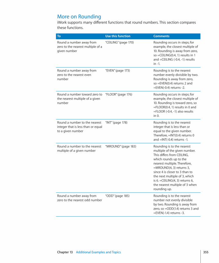
Chapter 13 Additional Examples and Topics 355
More on RoundingiWork supports many different functions that round numbers. This section compares these functions.
To Use this function Comments
Round a number away from zero to the nearest multiple of a given number
“CEILING” (page 170) Rounding occurs in steps; for example, the closest multiple of 10. Rounding is away from zero, so =CEILING(0.4, 1) results in 1 and =CEILING (-0.4, -1) results in -1.
Round a number away from zero to the nearest even number
“EVEN” (page 173) Rounding is to the nearest number evenly divisible by two. Rounding is away from zero, so =EVEN(0.4) returns 2 and =EVEN(-0.4) returns -2.
Round a number toward zero to the nearest multiple of a given number
“FLOOR” (page 176) Rounding occurs in steps; for example, the closest multiple of 10. Rounding is toward zero, so =FLOOR(0.4, 1) results in 0 and =FLOOR (-0.4, -1) also results in 0.
Round a number to the nearest integer that is less than or equal to a given number
“INT” (page 178) Rounding is to the nearest integer that is less than or equal to the given number. Therefore, =INT(0.4) returns 0 and =INT(-0.4) returns -1.
Round a number to the nearest multiple of a given number
“MROUND” (page 183) Rounding is to the nearest multiple of the given number. This differs from CEILING, which rounds up to the nearest multiple. Therefore, =MROUND(4, 3) returns 3, since 4 is closer to 3 than to the next multiple of 3, which is 6. =CEILING(4, 3) returns 6, the nearest multiple of 3 when rounding up.
Round a number away from zero to the nearest odd number
“ODD” (page 185) Rounding is to the nearest number not evenly divisible by two. Rounding is away from zero, so =ODD(1.4) returns 3 and =EVEN(-1.4) returns -3.

To Use this function Comments
Round a number to the specified number of places
“ROUND” (page 191) A positive number indicates the number of digits (decimal places) to the right of the decimal separator to include in the rounded number. A negative number indicates the number of digits to the left of the decimal separator to replace with zeros (the number of zeros at the end of the number). The number is rounded based on this. So =ROUND(1125, -2) returns 1,100 and =ROUND(1155, -2) returns 1,200. Rounding is away from zero, so =ROUND(-1125, -2) returns -1,100 and =ROUND(-1155, -2) returns -1,200.
Round a number down (toward zero) to the specified number of places
“ROUNDDOWN” (page 192) A positive number indicates the number of digits (decimal places) to the right of the decimal separator to include in the rounded number. A negative number indicates the number of digits to the left of the decimal separator to replace with zeros (the number of zeros at the end of the number). The number is rounded based on this. So =ROUND(1125, -2) returns 1,100 and =ROUND(1155, -2) also returns 1,100, since rounding is toward zero. =ROUND(-1125, -2) returns -1,100 and =ROUND(-1155, -2) also returns -1,100.
356 Chapter 13 Additional Examples and Topics

Chapter 13 Additional Examples and Topics 357
To Use this function Comments
Round a number up (away from zero) to the specified number of places
“ROUNDUP” (page 193) A positive number indicates the number of digits (decimal places) to the right of the decimal separator to include in the rounded number. A negative number indicates the number of digits to the left of the decimal separator to replace with zeros (the number of zeros at the end of the number). The number is rounded based on this. So =ROUND(1125, -2) returns 1,200 and =ROUND(1155, -2) also returns 1,200, since rounding is away from zero. =ROUND(-1125, -2) returns -1,200 and =ROUND(-1155, -2) also returns -1,200.
Truncate a number at the specified number of places
“TRUNC” (page 204) A positive number indicates the number of digits (decimal places) to the right of the decimal separator to include in the number. A negative number indicates the number of digits to the left of the decimal separator to replace with zeros (the number of zeros at the end of the number). Extra digits are stripped from the number. So =TRUNC(1125, -2) returns 1,100 and =TRUNC(1155, -2) also returns 1,100.

Using Logical and Information Functions TogetherLogical and information functions are often used together in a formula. Although logical functions are used independently, it is rare for an information function to be used on its own. This section includes more complex examples to illustrate how the use of several logical and information functions in a single formula can be very powerful.
Adding Comments Based on Cell ContentsThis example uses IF, AND, OR, and ISBLANK to add comments to a table based on existing cell contents. The IF function is quite powerful, especially when combined with other logical functions like OR and AND.
Assume that you are a college professor and one of the graduate assistants has handed you a table containing the names of students and their recent exam results. You want to quickly identify the following situations:
The student passed, but should come in for a special study session (score in the Ârange 61–75).
There is an error (negative test score, a test score over 100, or no test score) in the Âdata.
The student failed the exam (score of 60 or below). Â
Breaking this into parts, the functions below will determine each of the things you wish to know. When put together, you will be able to quickly glance at the table and see the desired information. For purposes of the expressions below, assume the first student’s name is in cell A2, and the first test score in cell B2.
358 Chapter 13 Additional Examples and Topics

Chapter 13 Additional Examples and Topics 359
Expression 1=AND(B2>60, B2<=75) tests for a low score. If the test score is in the range 61 to 75, AND will return TRUE meaning the student should come in for a special study session. Otherwise it will return FALSE.
Expression 2=OR(ISBLANK(B2), B2<0, B2>100) tests for invalid data. The first OR expression “ISBLANK(B2)” will be TRUE if there is no test score. The second expression will return TRUE if the test score is negative and the third expression will return TRUE if the test score is over 100. The OR will return TRUE if any of the conditions is TRUE, meaning the data is invalid in some way. The OR will return FALSE if none of the conditions are TRUE and therefore the data is valid.
Expression 3=B2<=60 tests for a failing grade. This expression will return TRUE if the test score is 60 or below, a failing grade. Otherwise it returns FALSE.
Putting it together in an IF function=IF(AND(B2>60, B2<=75), “Needs study session”, IF(OR(ISBLANK(B2), B2<0, B2>100), “Invalid data”, IF(B2<=60, “Exam failed”, “”)))
If the test expression (same as Expression 1 above) in the first IF evaluates to TRUE, the function will return “Needs study session”; otherwise it will continue to the FALSE argument, the second IF.
If the test expression (same as Expression 2 above) of the second IF evaluates to TRUE, the function will return “Invalid data”; otherwise it will continue to the FALSE argument, the third IF.
If the test expression (same as Expression 3 above) of the third IF evaluates to TRUE, the function will return “Exam failed”; otherwise the expression will return an empty expression (“”).
The result might look like the following table.

Trapping Division by ZeroSometimes it is not possible to construct a table in a manner that can avoid division by zero. However, if division by zero occurs, the result is an error value in the cell, which is usually not the desired result. This example shows three methods of preventing this error.
Examples
Assume that cell D2 and E2 each contain a number. It is possible that E2 contains 0. You wish to divide D2 by E2, but avoid a division by zero error. Each of the following three methods will return 0 if cell E2 is equal to zero; otherwise each returns the result of D2/E2.
=IF(E2=0,0,D2/E2) operates by directly testing cell E2 to see if it is 0.
=IFERROR(D2/E2,0) operates by returning 0 if an error occurs. Division by zero is an error.
=IF(ISERROR(D2/E2),0,D2/E2) operates by doing a logical test to see if D2/E2 is TRUE.
Specifying Conditions and Using WildcardsSome functions, such as SUM, operate on entire ranges. Other functions, such as SUMIF, only operate on the cells in the range that meet a condition. For example you might want to add up all the numbers in column B that are less than 5. To do this, you could use =SUMIF(B, “<5”). The second argument of SUMIF is called a condition because it causes the function to ignore cells that do not meet the requirements.
There are two types of functions that take conditions. The first type is functions that have names ending in IF or IFS (except for the function IF, which does not take a condition; it instead takes an expression that should evaluate to either TRUE or FALSE). These functions can do numeric comparisons in their conditions, such as “>5”, “<=7”, or “<>2”. These functions also accept wildcards in specifying conditions. For example, to count the number of cells in column B that begin with the letter “a”, you could use =COUNTIF(B, “a*”)
The second group of functions take conditions, such as HLOOKUP, but can’t do numeric conditions. These functions sometimes permit the use of wildcards.
Function Allows numeric comparisons Accepts wildcards
AVERAGEIF yes yes
AVERAGEIFS yes yes
COUNTIF yes yes
COUNTIFS yes yes
SUMIF yes yes
SUMIFS yes yes
360 Chapter 13 Additional Examples and Topics

Chapter 13 Additional Examples and Topics 361
Function Allows numeric comparisons Accepts wildcards
HLOOKUP no if exact match specified
MATCH no if exact match specified
VLOOKUP no if exact match specified
Examples of conditions, both with and without wildcards, are illustrated in this section.
Expression Example
“>4” means match any number greater than 4. =COUNTIF(B2:E7, “>4”) returns a count of the number of cells in the range B2:E7 that contain a value greater than 4.
“>=7” means match any number greater than or equal to 7.
=SUMIF(B, “>=7”) sums the cells in the column B that contain a value greater than or equal to 7.
“<=5” in combination with “>=15” means match any number less than or equal to 5 or greater than or equal to 15. Numbers 6 through 14, inclusive, would not be included.
=SUMIF(A3:B12,”<=5”)+SUMIF(A3:B12,”>=15”) sums the cells in the range A3:B12 that contain a value less than or equal to 5 or greater than or equal to 15.
“*it” means any value that ends with “it.” The asterisk (*) matches any number of characters.
=COUNTIF(B2:E7, “*it”) returns a count of the number of cells in the range B2:E7 that contain a value that ends with “it” such as “bit” and “mit.” It does not match “mitt.”
“~*” means to match the asterisk (*). The tilde (~) character means to take the next character literally, instead of treating it as a wildcard.
=COUNTIF(E, “~*”) returns a count of the number of cells in column E that contain the asterisk character.
B2 & “, “ & E2 returns the contents of cells B2 and E2 separated by a comma and a space.
=B2&”, “&E2 returns “Last, First” if B2 contains “Last” and E2 contains “First.”
“?ip” means any value that begins with a single character followed by “ip.”
=COUNTIF(B2:E7, “?ip”) returns a count of the number of cells in the range B2:E7 that contain a value that starts with a character followed by “ip” such as “rip” and “tip.” It does not match “drip” or “trip.”
“~?” means to match the question mark (?). The tilde (~) character means to take the next character literally, instead of treating it as a wildcard.
=SEARCH(“~?”, B2) returns 19 if cell B2 contains “This is a question? Yes it is.”, since the question mark is the 19th character in the string.
“*on?” means to match any value that begins with any number of characters followed by “on” and then a single character.
=COUNTIF(B2:E7, “*on?”) returns a count of the number of cells in the range B2:E7 that contain a value that starts with any number of characters (including none) followed by “on” and then a single character. This matches words such as “alone”, “bone”, “one”, and “none.” This does not match “only” (has two characters after the “on”) or “eon” (has no characters after the “on”).

Survey Results ExampleThis example brings together the illustrations used throughout the statistical functions. It is based on a hypothetical survey. The survey was short (only five questions) and had a very limited number of respondents (10). Each question could be answered on a scale of 1 to 5 (perhaps the range from “never” to “always”), or not answered. Each survey was assigned a number before mailing. The following table shows the results. Questions that were answered outside the range (incorrect) or not answered are indicated with a blank cell in the table.
To illustrate some of the functions, assume that the survey control number included an alphabetic prefix and that the scale was A–E, instead of 1–5. The table would then look like this:
Using this table of data and some of the statistical functions available in iWork, you can gather information about the survey results. Keep in mind that the example is purposely small so results may seem obvious. However, if you had 50, 100, or more respondents and perhaps many more questions, the results would not be obvious.
362 Chapter 13 Additional Examples and Topics

Chapter 13 Additional Examples and Topics 363
Function and arguments Description of result
=CORREL(B2:B11, C2:C11) Determines the correlation of question 1 and question 2 using linear regression analysis. Correlation is a measure of how much two variables (in this case, answers to survey questions) change together. Specifically, this would look at the question: If a respondent answered question 1 with a higher (or lower) value than the average for question 1, did the respondent also answer question 2 with a higher (or lower) value than the average for question 2? In this case, the responses are not particularly well correlated (-0.1732)
=COUNT(A2:A11) or =COUNTA(A2:A11) Determines the total number of surveys returned (10). Note that if the survey control identifier was not numeric, you would need to use COUNTA instead of COUNT.
=COUNT(B2:B11) or =COUNTA(B2:B11) Determines the total number of responses to the first question (9). By extending this formula across the row, you could determine the total number of responses to each question. Because all the data is numeric, COUNTA returns the same results. If, however, the survey had used A through E, instead of 1 through 5, you would need to use COUNTA to tally the results.
=COUNTBLANK(B2:B11) Determines the number of empty cells, representing invalid or no answers. If you extended this formula across the row you would find that question 3 (column D) had 3 invalid or not-answered responses. This might cause you to look at this question on the survey to see if it was controversial or poorly worded, as no other question had more than 1 incorrect or not-answered response.
=COUNTIF(B2:B11, “=5”) Determines the number of respondents that gave a 5 to a particular question (in this case, question 1). If you extended this formula across the row, you would learn that only questions 1 and 4 had any respondents give the question a 5. Had the survey used A through E for the range, you would have used =COUNTIF(B2:B11, “=E”).

Function and arguments Description of result
=COVAR(B2:B11, C2:C11) Determines the covariance of question 1 and question 2. Covariance is a measure of how much two variables (in this case, answers to survey questions) change together. Specifically, this would look at the question: If a respondent answered question 1 with a higher (or lower) value than the average for question 1, did the respondent also answer question 2 with a higher (or lower) value than the average for question 2?
Note: COVAR would not work with the table using a scale of A–E, as it requires numeric arguments.
=STDEV(B2:B11) or =STDEVP(B2:B11) Determines the standard deviation, one measure of dispersion, of the answers to question 1. If you extend this formula across the row, you would see that the answers to question 3 had the highest standard deviation. If the results represented responses from the entire population being studied, rather than a sample, STDEVP would be used instead of STDEV. Note that STDEV is the square root of VAR.
=VAR(B2:B11) or =VARP(B2:B11) Determines the variance, one measure of dispersion, of the answers to question 1. If you extended this formula across the row, you would see that the answers to question 5 had the lowest variance. If the results represented responses from the entire population being studied, rather than a sample, VARP would be used instead of VAR. Note that VAR is the square of STDEV.
364 Chapter 13 Additional Examples and Topics

Inde
x
365
Index
Symbols? wildcard 30, 361* wildcard 30, 361& string operator 30, 310~ wildcard escape character 30, 361
AABS numeric function 170absolute cell references 27ACCRINT financial function 99, 351ACCRINTM financial function 101ACOS trigonometric function 327ACOSH trigonometric function 328ADDRESS reference function 207ampersand string operator 30, 310AND logical and information function 156, 358any value type 36AREAS reference function 209arithmetic operators 28array constant 35array defined 35array function
defined 35FREQUENCY 257INDEX 214INDIRECT 216LINEST 265OFFSET 219TRANSPOSE 222
ASIN trigonometric function 329ASINH trigonometric function 329asterisk wildcard 30, 361ATAN trigonometric function 330ATAN2 trigonometric function 331ATANH trigonometric function 332AVEDEV statistical function 230AVERAGE statistical function 231AVERAGEA statistical function 232AVERAGEIF statistical function 233, 360AVERAGEIFS statistical function 234, 360
BBASETONUM engineering function 73
BESSELJ engineering function 74BESSELY engineering function 75BETADIST statistical function 236BETAINV statistical function 237BIN2DEC engineering function 76BIN2HEX engineering function 77BIN2OCT engineering function 78BINOMDIST statistical function 238bond investment related financial questions 351BONDDURATION financial function 103BONDMDURATION financial function 104Boolean expression defined 35Boolean value type 36
Ccalculations, instant 17CEILING numeric function 170, 355cell comments example 358cell references
distinguishing absolute and relative 27inserting into formulas 26
CHAR text function 308CHIDIST statistical function 239CHIINV statistical function 239CHITEST statistical function 240CHOOSE reference function 209choosing which TVM function to use 348CLEAN text function 308CODE text function 309collection value type 36colon as reference element separator 39COLUMN reference function 210COLUMNS reference function 211COMBIN numeric function 172commas as argument separators 34common arguments used in financial functions 341comparison operators 29CONCATENATE text function 310condition 30
comparison operators 29defined 35specifying 360
CONFIDENCE statistical function 242
Index
Inde
x

366 Index
constant defined 35conversion units
distance 80duration 80energy 81force 81liquid 82magnetism 82metric prefixes 83power 82pressure 81speed 81temperature 82weight and mass 80
CONVERT engineering function 79copying help examples into a table 41CORREL statistical function 242, 363COS trigonometric function 333COSH trigonometric function 334COUNT statistical function 244, 363COUNTA statistical function 245, 363COUNTBLANK statistical function 246, 363COUNTIF statistical function 247, 360, 361, 363COUNTIFS statistical function 248, 253, 360COUPDAYBS financial function 105COUPDAYS financial function 107COUPDAYSNC financial function 108COUPNUM financial function 109, 351COVAR statistical function 250, 364CRITBINOM statistical function 252CUMIPMT financial function 110, 112, 349CUMPRINC financial function 349
Ddate and time function
DATE 44DATEDIF 45DATEVALUE 47DAY 47DAYNAME 48DAYS360 49EDATE 50EOMONTH 51HOUR 51MINUTE 52MONTH 53MONTHNAME 54NETWORKDAYS 54NOW 55SECOND 56TIME 56TIMEVALUE 57TODAY 58WEEKDAY 59WEEKNUM 60WORKDAY 61
YEAR 62YEARFRAC 63
DATE date and time function 44DATEDIF date and time function 45date/time value type 36DATEVALUE date and time function 47DAY date and time function 47DAYNAME date and time function 48DAYS360 date and time function 49DB financial function 114, 352DDB financial function 116, 352DEC2BIN engineering function 83DEC2HEX engineering function 84DEC2OCT engineering function 85DEGREES trigonometric function 334DELTA engineering function 86depreciation-related financial questions 352DEVSQ statistical function 253DISC financial function 117, 351distance conversion units 80DOLLAR financial function 311double colon as reference element separator 39DUR2DAYS duration function 65DUR2HOURS duration function 65DUR2MILLISECONDS duration function 66DUR2MINUTES duration function 67DUR2SECONDS duration function 68DUR2WEEKS duration function 69duration conversion units 80DURATION duration function 70duration function
DUR2DAYS 65DUR2HOURS 65DUR2MILLISECONDS 66DUR2MINUTES 67DUR2SECONDS 68DUR2WEEKS 69DURATION 70STRIPDURATION 71
duration value type 37
EEDATE date and time function 50EFFECT financial function 119, 351ellipsis syntax elements 35energy conversion units 81engineering function
BASETONUM 73BESSELJ 74BESSELY 75BIN2DEC 76BIN2HEX 77BIN2OCT 78CONVERT 79DEC2BIN 83DEC2HEX 84
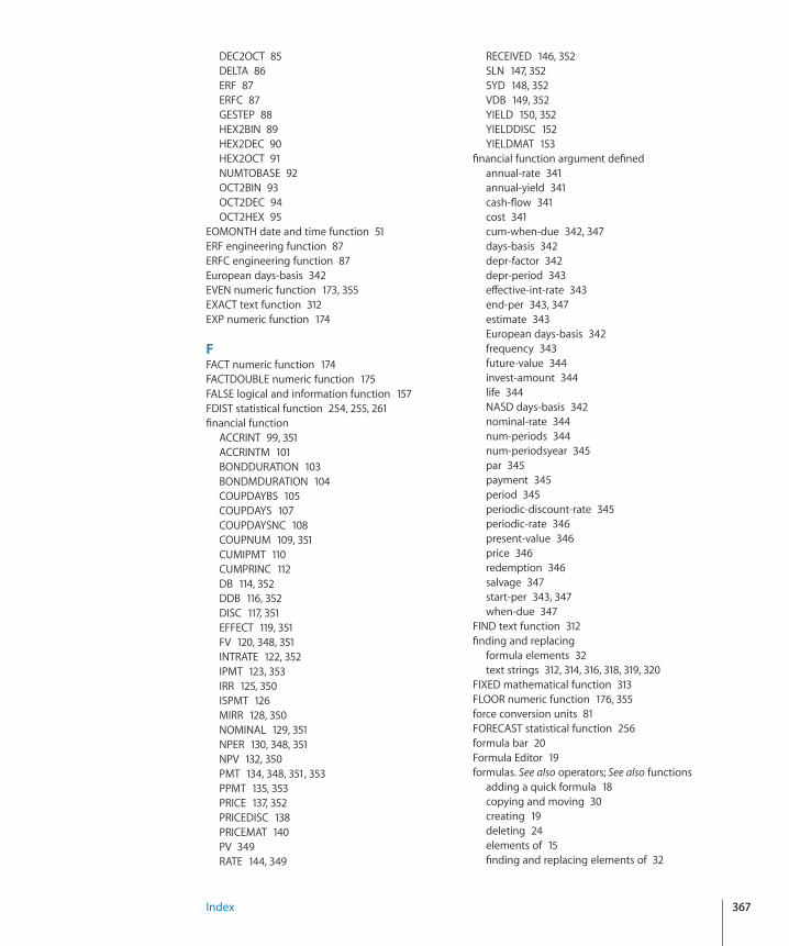
Index 367
DEC2OCT 85DELTA 86ERF 87ERFC 87GESTEP 88HEX2BIN 89HEX2DEC 90HEX2OCT 91NUMTOBASE 92OCT2BIN 93OCT2DEC 94OCT2HEX 95
EOMONTH date and time function 51ERF engineering function 87ERFC engineering function 87European days-basis 342EVEN numeric function 173, 355EXACT text function 312EXP numeric function 174
FFACT numeric function 174FACTDOUBLE numeric function 175FALSE logical and information function 157FDIST statistical function 254, 255, 261financial function
ACCRINT 99, 351ACCRINTM 101BONDDURATION 103BONDMDURATION 104COUPDAYBS 105COUPDAYS 107COUPDAYSNC 108COUPNUM 109, 351CUMIPMT 110CUMPRINC 112DB 114, 352DDB 116, 352DISC 117, 351EFFECT 119, 351FV 120, 348, 351INTRATE 122, 352IPMT 123, 353IRR 125, 350ISPMT 126MIRR 128, 350NOMINAL 129, 351NPER 130, 348, 351NPV 132, 350PMT 134, 348, 351, 353PPMT 135, 353PRICE 137, 352PRICEDISC 138PRICEMAT 140PV 349RATE 144, 349
RECEIVED 146, 352SLN 147, 352SYD 148, 352VDB 149, 352YIELD 150, 352YIELDDISC 152YIELDMAT 153
financial function argument definedannual-rate 341annual-yield 341cash-flow 341cost 341cum-when-due 342, 347days-basis 342depr-factor 342depr-period 343effective-int-rate 343end-per 343, 347estimate 343European days-basis 342frequency 343future-value 344invest-amount 344life 344NASD days-basis 342nominal-rate 344num-periods 344num-periodsyear 345par 345payment 345period 345periodic-discount-rate 345periodic-rate 346present-value 346price 346redemption 346salvage 347start-per 343, 347when-due 347
FIND text function 312finding and replacing
formula elements 32text strings 312, 314, 316, 318, 319, 320
FIXED mathematical function 313FLOOR numeric function 176, 355force conversion units 81FORECAST statistical function 256formula bar 20Formula Editor 19formulas. See also operators; See also functions
adding a quick formula 18copying and moving 30creating 19deleting 24elements of 15finding and replacing elements of 32

368 Index
handling errors and warnings 23inserting cell references 26operators 28performing instant calculations 17using arithmetic operators 28using cell references 24using comparison operators 29using the formula bar 20using the Formula Editor 19using the Function Browser 21viewing all in a spreadsheet 31
formulas that reference the same cell in multiple tables 39
FREQUENCY statistical function 257Function Browser 21. See also functionsfunctions. See also formulas
adding to formulas 21any value type defined 36array constant defined 35array defined 35array function defined 35Boolean expression defined 35Boolean value type defined 36collection value type defined 36colon and double colon separators 39comma and semicolon argument separators 34condition defined 35constant defined 35date and time 42date/time value type defined 36duration 64duration value type defined 37ellipsis syntax element 35engineering 72financial 96introduction to 33italic text 34list value type defined 38logical and information 155modal argument defined 35modal value type defined 38number value type defined 38numeric 167parentheses syntax element 34range value type defined 38reference 206reference value type defined 39statistical 225string value type defined 39syntax elements used in function definitions 34table spanning formulas 39text 306trigonometric 326uppercase text 34
FV financial function 120, 348, 351
GGAMMADIST statistical function 259GAMMAINV statistical function 260GAMMALN statistical function 260GCD numeric function 177GESTEP engineering function 88
HHARMEAN statistical function 262HEX2BIN engineering function 89HEX2DEC engineering function 90HEX2OCT engineering function 91HLOOKUP reference function 211, 361HOUR date and time function 51HYPERLINK reference function 213
IIF logical and information function 158, 358IF logical function 360IFERROR logical and information function 159IFERROR logical function 360INDEX reference function 214INDIRECT reference function 216instant calculations 17INT numeric function 178, 355INTERCEPT statistical function 262INTRATE financial function 122, 352introduction to functions 33IPMT financial function 123, 349, 353IRR financial function 125, 350ISBLANK logical and information function 160, 358ISERROR logical and information function 161ISERROR logical function 360ISEVEN logical and information function 162ISODD logical and information function 163ISPMT financial function 126italic text syntax elements 34
LLARGE statistical function 264LCM numeric function 179LEFT text function 314LEN text function 315LINEST additional statistics 267LINEST statistical function 265liquid conversion units 82list value type 38LN numeric function 179loan amortization table 353loan related financial questions 351LOG numeric function 180LOG10 numeric function 181logical and information function
AND 156, 358FALSE 157

Index 369
IF 158, 358IFERROR 159ISBLANK 160, 358iserror 161ISEVEN 162ISODD 163NOT 164OR 165, 358TRUE 166
LOGINV statistical function 268LOGNORMDIST statistical function 269LOOKUP reference function 217LOWER text function 316
Mmagnetism conversion units 82MATCH reference function 218, 361MAX statistical function 270MAXA statistical function 270MEDIAN statistical function 271metric prefixes for conversion units 83MID text function 316MIN statistical function 272MINA statistical function 273MINUTE date and time function 52MIRR financial function 128, 350MOD numeric function 182modal argument defined 35modal value type 38MODE statistical function 274MONTH date and time function 53MONTHNAME date and time function 54MROUND numeric function 183, 355MULTINOMIAL numeric function 184
NNASD days-basis method 342navigating to table cells referenced in formulas 26NEGBINOMDIST statistical function 275NETWORKDAYS date and time function 54NOMINAL financial function 129, 351NORMDIST statistical function 276NORMINV statistical function 277NORMSDIST statistical function 277NORMSINV statistical function 278NOT logical and information function 164NOW date and time function 55NPER financial function 130, 348, 351NPV financial function 132, 350number value type 38numeric function
CEILING 355EVEN 355FLOOR 355INT 355MROUND 355
ODD 355ROUND 356ROUNDDOWN 356ROUNDUP 357TRUNC 357
numeric functionsABS 170CEILING 170COMBIN 172EVEN 173EXP 174FACT 174FACTDOUBLE 175FLOOR 176GCD 177INT 178LCM 179LN 179LOG 180LOG10 181MOD 182MROUND 183MULTINOMIAL 184ODD 185PI 186POWER 186PRODUCT 187QUOTIENT 188RAND 189RANDBETWEEN 189ROMAN 190ROUND 191ROUNDDOWN 192ROUNDUP 193SIGN 195SQRT 195SQRTPI 196SUM 196SUMIF 197, 360SUMIFS 198, 360SUMPRODUCT 200SUMSQ 201SUMX2MY2 202SUMX2PY2 203SUMXMY2 204TRUNC 204
NUMTOBASE mathematical function 92
OOCT2BIN engineering function 93OCT2DEC engineering function 94OCT2HEX engineering function 95ODD numeric function 185, 355OFFSET reference function 219operators
arithmetic 28

370 Index
comparison 29string 30, 310
OR logical and information function 165, 358
Pparentheses syntax elements 34pasting help examples into a table 41PERCENTILE statistical function 279PERCENTRANK statistical function 280PERMUT statistical function 281PI numeric function 186PMT financial function 134, 348, 351, 353POISSON statistical function 282power conversion units 82POWER numeric function 186PPMT financial function 135, 349, 353pressure conversion units 81PRICE financial function 137, 352PRICEDISC financial function 138PRICEMAT financial function 140PROB statistical function 282PRODUCT numeric function 187PROPER text function 317PV financial function 141, 349
QQUARTILE statistical function 284question mark wildcard 30, 361quick formulas 18QUOTIENT numeric function 188
RRADIANS trigonometric function 335RAND numeric function 189RANDBETWEEN numeric function 189range value type 38RANK statistical function 285RATE financial function 144, 349RECEIVED financial function 146, 352reference function
ADDRESS 207AREAS 209CHOOSE 209COLUMN 210COLUMNS 211HLOOKUP 211, 361HYPERLINK 213INDEX 214INDIRECT 216LOOKUP 217MATCH 218, 361OFFSET 219ROW 221ROWS 221TRANSPOSE 222
VLOOKUP 223, 361reference value type 39referencing the same cell in multiple tables 39regular expressions using wildcards 361relative cell references 27REPLACE text function 318REPT text function 319RIGHT text function 319ROMAN numeric function 190ROUND numeric function 191, 356ROUNDDOWN numeric function 192, 356rounding 355ROUNDUP numeric function 193, 357ROW reference function 221ROWS reference function 221
Ssavings related financial questions 351search expressions 361SEARCH text function 320, 361searching for formulas. See finding and replacingSECOND date and time function 56semicolons as argument separators 34SIGN numeric function 195SIN trigonometric function 336SINH trigonometric function 337SLN financial function 147, 352SLOPE statistical function 287SMALL statistical function 288solving common financial questions 351speed conversion units 81spreadsheets
finding and replacing formula elements 32viewing all formulas in 31
SQRT numeric function 195SQRTPI numeric function 196STANDARDIZE statistical function 289statistical function
AVEDEV 230AVERAGE 231AVERAGEA 232AVERAGEIF 233, 360AVERAGEIFS 234, 360BETADIST 236BETAINV 237BINOMDIST 238CHIDIST 239CHIINV 239CHITEST 240CONFIDENCE 242CORREL 242, 363COUNT 244, 363COUNTA 245, 363COUNTBLANK 246, 363COUNTIF 247, 360, 363COUNTIFS 248, 360

Index 371
COVAR 250, 364CRITBINOM 252DEVSQ 253EXPONDIST 253FDIST 254FINV 255FORECAST 256FREQUENCY 257GAMMADIST 259GAMMAINV 260GAMMALN 260GEOMEAN 261HARMEAN 262INTERCEPT 262LARGE 264LINEST 265LOGINV 268LOGNORMDIST 269MAX 270MAXA 270MEDIAN 271MIN 272MINA 273MODE 274NEGBINOMDIST 275NORMDIST 276NORMINV 277NORMSDIST 277NORMSINV 278PERCENTILE 279PERCENTRANK 280PERMUT 281POISSON 282PROB 282QUARTILE 284RANK 285SLOPE 287SMALL 288STANDARDIZE 289STDEV 290, 364STDEVA 291STDEVP 293, 364STDEVPA 294TDIST 296TINV 297TTEST 297VAR 298, 364VARA 300VARP 302, 364VARPA 303ZTEST 305
STDEV statistical function 290, 364STDEVA statistical function 291STDEVP statistical function 293, 364STDEVPA statistical function 294string operator 30
string value type 39STRIPDURATION duration function 71SUBSTITUTE text function 322SUM numeric function 196SUMIF mathematical function 360SUMIF numeric function 197, 361SUMIFS numeric function 198, 360SUMPRODUCT numeric function 200SUMSQ numeric function 201SUMX2MY2 numeric function 202SUMX2PY2 numeric function 203SUMXMY2 numeric function 204survey results example 362SYD financial function 148, 352syntax elements used in function definitions 34
TT text function 323table spanning formulas 39TAN trigonometric function 338TANH trigonometric function 339TDIST statistical function 296temperature conversion units 82text function
CHAR 308CLEAN 308CODE 309CONCATENATE 310DOLLAR 311EXACT 312FIND 312FIXED 313LEFT 314LEN 315LOWER 316MID 316PROPER 317REPLACE 318REPT 319RIGHT 319SEARCH 320SUBSTITUTE 322T 323TRIM 323UPPER 324VALUE 325
tilde wildcard escape character 30, 361TIME date and time function 56TIMEVALUE date and time function 57TINV statistical function 297TODAY date and time function 58TRANSPOSE reference function 222trapping division by zero 360trigonometric function
ACOS 327ACOSH 328

372 Index
ASIN 329ASINH 329ATAN 330ATAN2 331ATANH 332COS 333COSH 334DEGREES 334RADIANS 335SIN 336SINH 337TAN 338TANH 339
TRIM text function 323TRUE logical and information function 166TRUNC numeric function 204, 357TTEST statistical function 297
UUPPER text function 324uppercase text syntax elements 34using a formula to reference the same cell in
multiple tables 39using help examples in a table 41using logical and information functions
together 358
VVALUE text function 325value types
any 36Boolean 36collection 36date/time 36duration 37list 38modal 38number 38range 38reference 39string 39
VAR statistical function 298, 364VARA statistical function 300VARP statistical function 302, 364VARPA statistical function 303VDB financial function 149, 352VLOOKUP reference function 223, 361
WWEEKDAY date and time function 59WEEKNUM date and time function 60weight and mass conversion units 80wildcards 30, 360, 361WORKDAY date and time function 61working with help example tables 41
YYEAR date and time function 62YEARFRAC date and time function 63YIELD financial function 150, 352YIELDDISC financial function 152YIELDMAT financial function 153
Zzero coupon bond 351ZTEST statistical function 305