1

IPST 2015 / Dubrovnik15-18 June 2015

History of Transient Analysis, EMTP Development and IPST

A. Ametani, Ecole Polytechnique Montreal, Canada

1. Background of transient analysis 2. Computer simulations3. EMTP4. Numerical Electromagnetic Analysis5. IPST

2

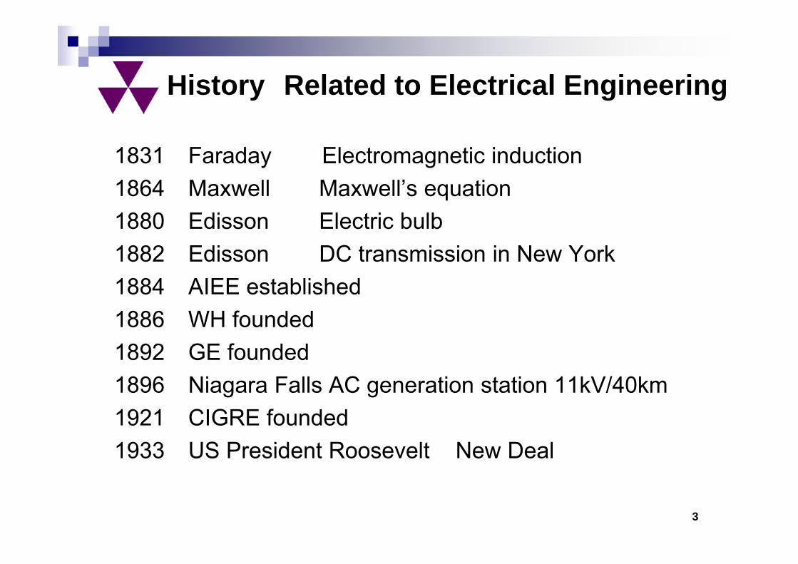
1831 Faraday Electromagnetic induction1864 Maxwell Maxwell’s equation1880 Edisson Electric bulb1882 Edisson DC transmission in New York1884 AIEE established1886 WH founded1892 GE founded1896 Niagara Falls AC generation station 11kV/40km1921 CIGRE founded1933 US President Roosevelt New Deal

3

History Related to Electrical Engineering

2

1. Background of Transient Analysis

(1) Trans - Atlantic tele - communication cable･Kelvin arrival curve in 1854･ wave (signal) distortion → Heaviside (Laplace) transform

in 1900s･ transient analysis in a lumped-parameter circuit

(2) US 220kV transmission line in 1923･ transformer failure due to lightning to the transmission

line : lightning overvoltage analysis→ Heaviside transform to a transformer

traveling wave theory to a transmission line･ transient analysis in a distributed-parameter circuit

3

(3) Fault surge (temporary overvoltage)→ symmetrical component theory in 1930s

･ modal analysis of a multi-phase line

(4) Telephone line interference in 1930s→ accurate impedance / admittance required

･conductor internal impedance by Schelknoffearth - return impedance by Pollaczeck and Carsonearth - return admittance by Wise

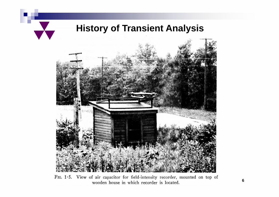
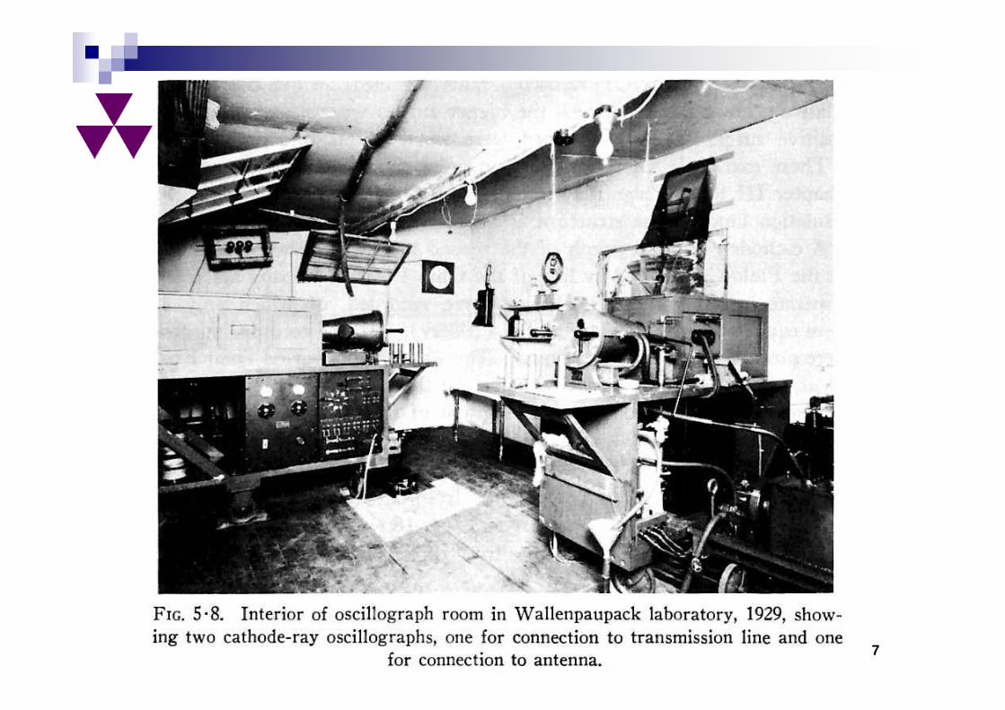
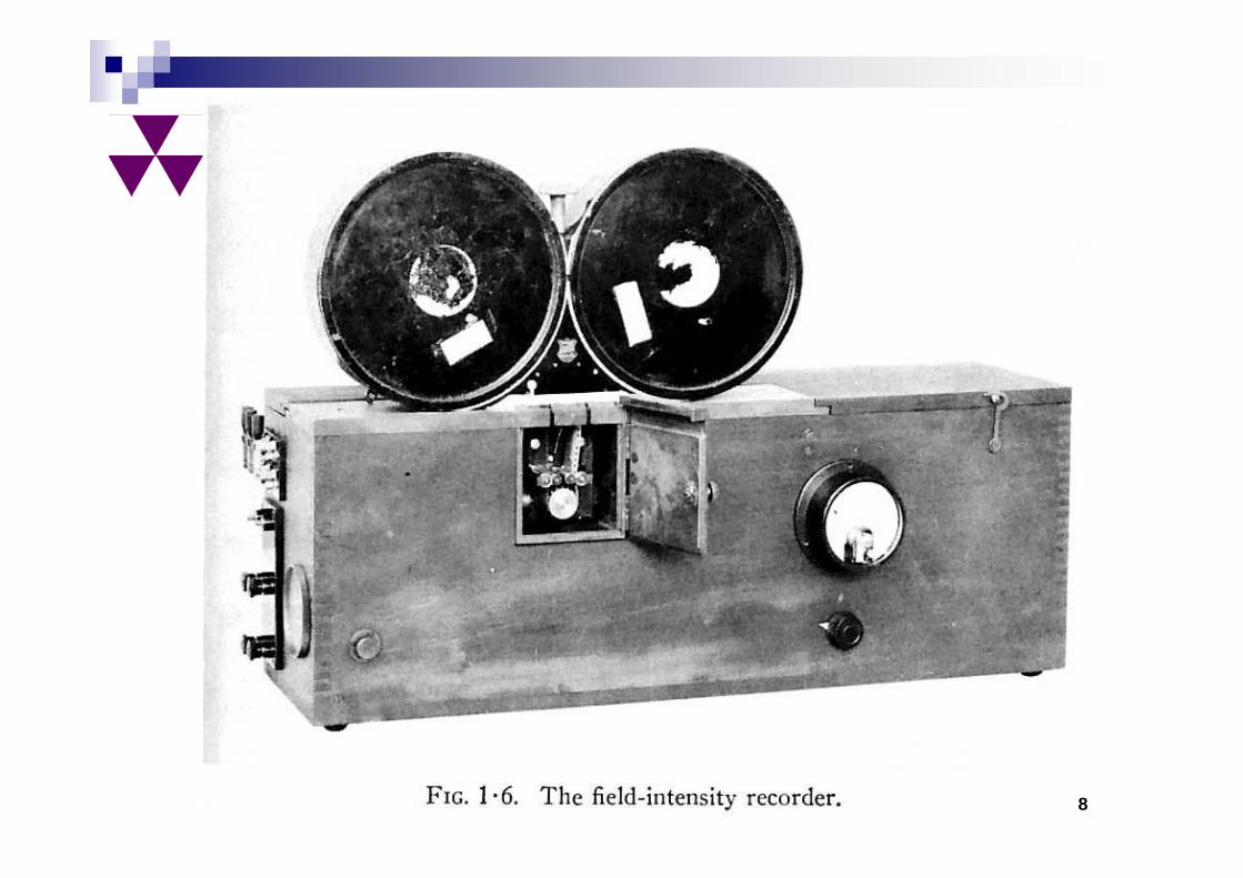
History of Transient Analysis

6

7

8

9

10

11

12

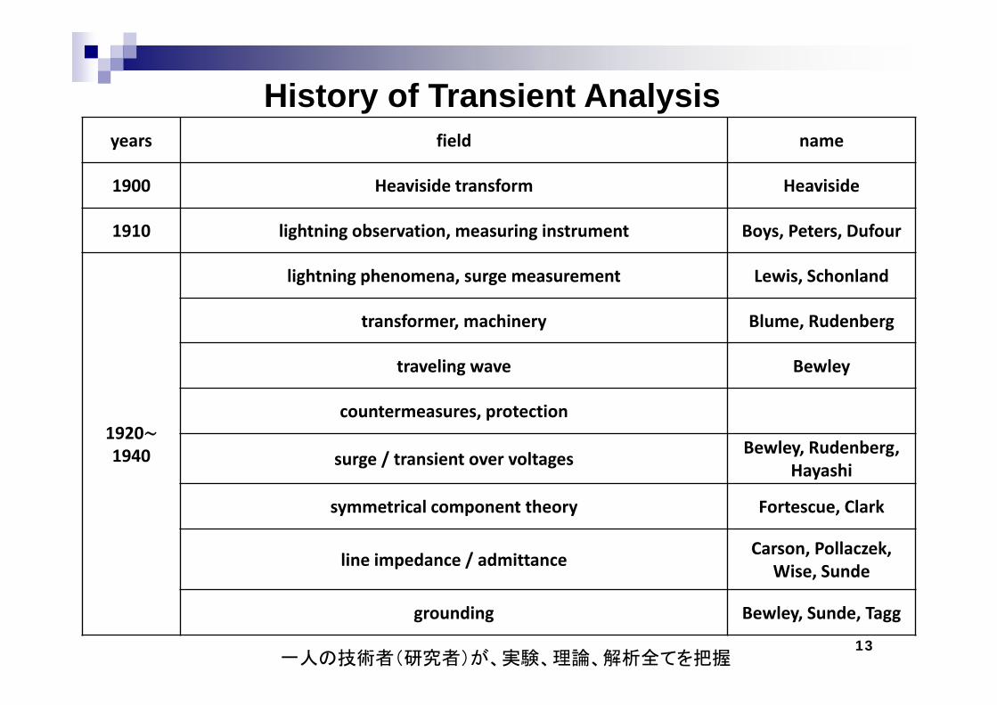
History of Transient Analysisyears field name

1900 Heaviside transform Heaviside

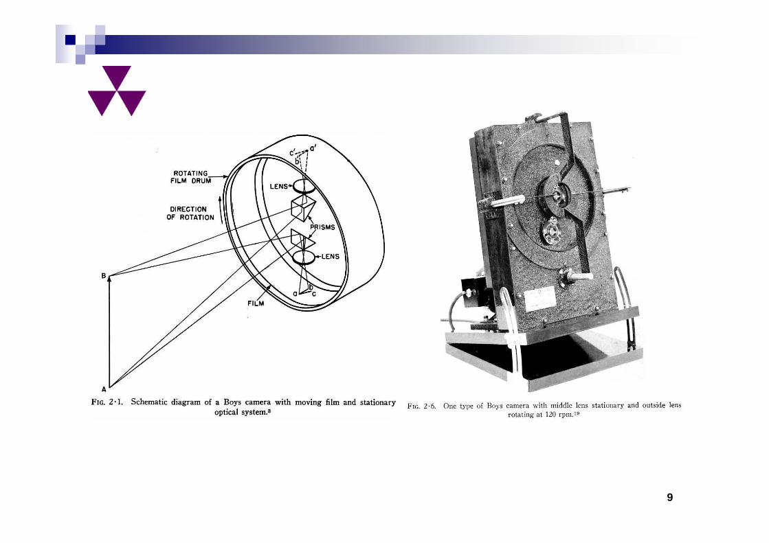
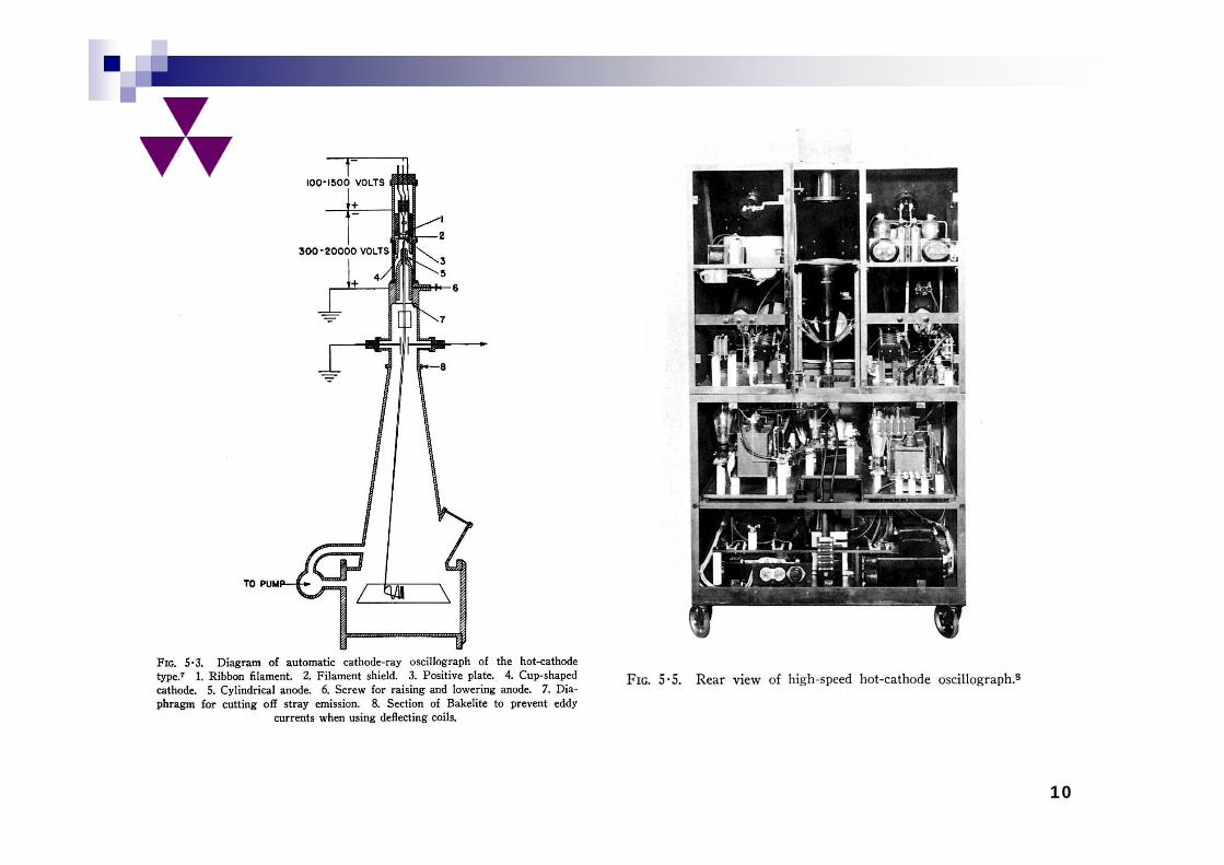
1910 lightning observation, measuring instrument Boys, Peters, Dufour

1920∼1940

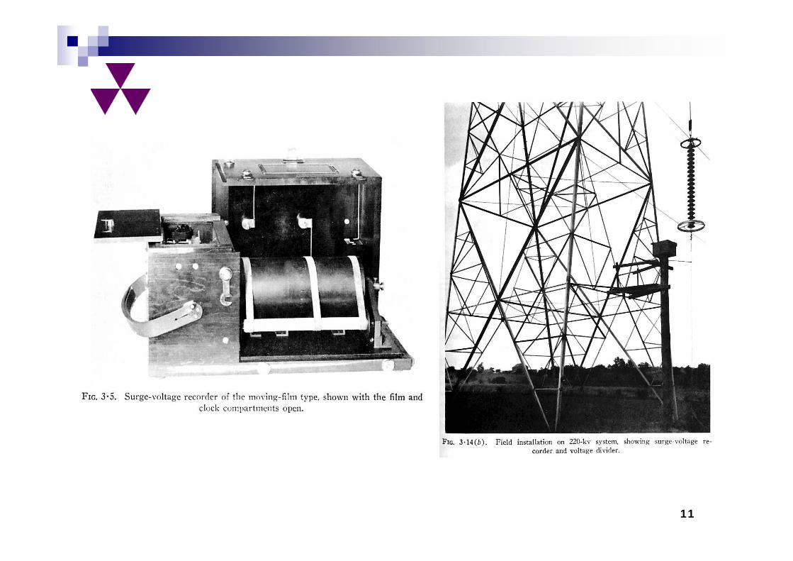
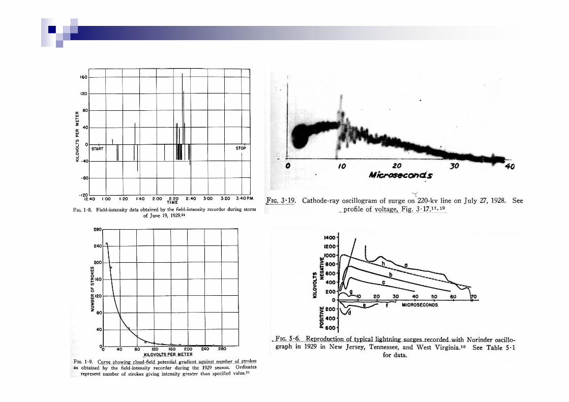
lightning phenomena, surge measurement Lewis, Schonland

transformer, machinery Blume, Rudenberg

traveling wave Bewley

countermeasures, protection

surge / transient over voltages Bewley, Rudenberg, Hayashi

symmetrical component theory Fortescue, Clark

line impedance / admittance Carson, Pollaczek, Wise, Sunde

grounding Bewley, Sunde, Tagg

一人の技術者（研究者）が、実験、理論、解析全てを把握13

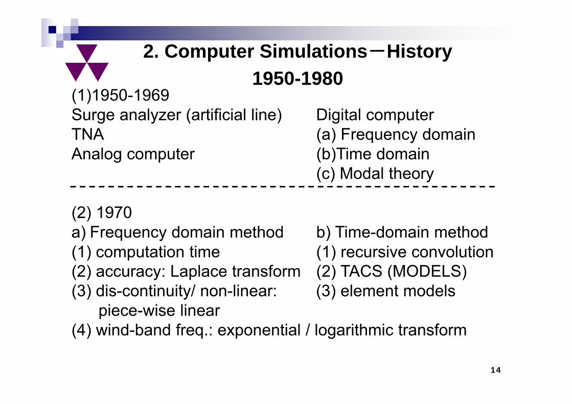
(1)1950-1969Surge analyzer (artificial line) Digital computerTNA (a) Frequency domainAnalog computer (b)Time domain

(c) Modal theory

(2) 1970a) Frequency domain method b) Time-domain method(1) computation time (1) recursive convolution(2) accuracy: Laplace transform (2) TACS (MODELS)(3) dis-continuity/ non-linear: (3) element models

piece-wise linear(4) wind-band freq.: exponential / logarithmic transform

2. Computer Simulations－History1950-1980

14

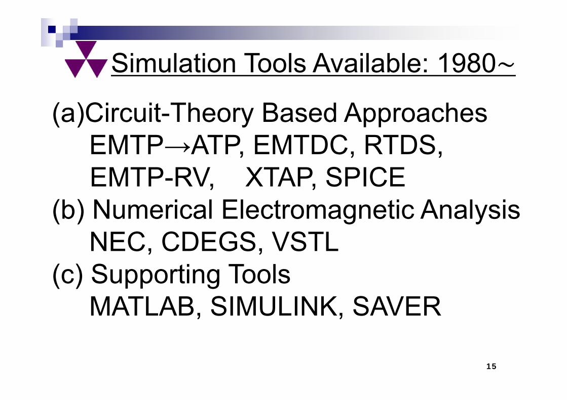
(a)Circuit-Theory Based ApproachesEMTP→ATP, EMTDC, RTDS, EMTP-RV, XTAP, SPICE

(b) Numerical Electromagnetic AnalysisNEC, CDEGS, VSTL

(c) Supporting ToolsMATLAB, SIMULINK, SAVER

Simulation Tools Available: 1980

15

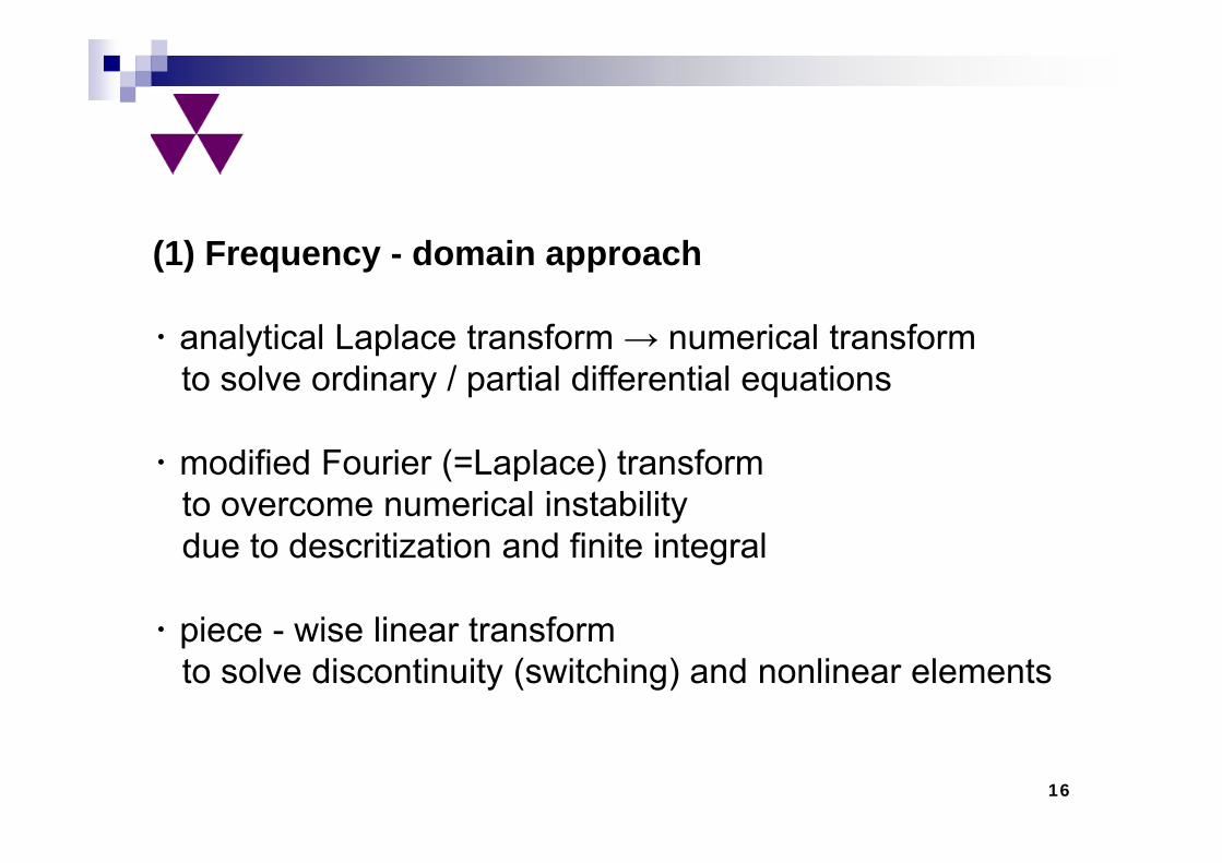
(1) Frequency - domain approach

･ analytical Laplace transform → numerical transformto solve ordinary / partial differential equations

･ modified Fourier (=Laplace) transformto overcome numerical instabilitydue to descritization and finite integral

･ piece - wise linear transformto solve discontinuity (switching) and nonlinear elements

16

(2) Time-domain approach

･ traveling wave theory based on Schnyder - Bergeron method to solve partial differential equations(method of characteristics)

･ real-time convolutionto deal with frequency-dependent parameters

17

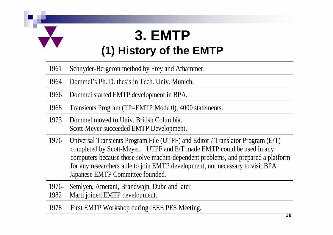
1961 Schnyder-Bergeron method by Frey and Athammer.

1964 Dommel’s Ph. D. thesis in Tech. Univ. Munich.

1966 Dommel started EMTP development in BPA.

1968 Transients Program (TP=EMTP Mode 0), 4000 statements. 1973 Dommel moved to Univ. British Columbia. Scott-Meyer succeeded EMTP Development. 1976 Universal Transients Program File (UTPF) and Editor / Translator Program (E/T)

completed by Scott-Meyer. UTPF and E/T made EMTP could be used in any computers because those solve machin-dependent problems, and prepared a platform for any researchers able to join EMTP development, not necessary to visit BPA.

Japanese EMTP Committee founded. 1976- Semlyen, Ametani, Brandwajn, Dube and later 1982 Marti joined EMTP development. 1978 First EMTP Workshop during IEEE PES Meeting.

3. EMTP (1) History of the EMTP

18

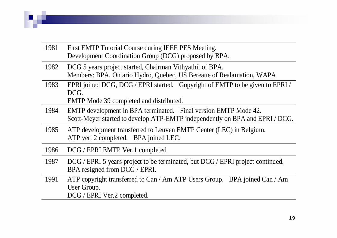
1981 First EMTP Tutorial Course during IEEE PES Meeting. Development Coordination Group (DCG) proposed by BPA. 1982 DCG 5 years project started, Chairman Vithyathil of BPA. Members: BPA, Ontario Hydro, Quebec, US Bereaue of Realamation, WAPA 1983 EPRl joined DCG, DCG / EPRI started. Gopyright of EMTP to be given to EPRI /

DCG. EMTP Mode 39 completed and distributed. 1984 EMTP development in BPA terminated. Final version EMTP Mode 42. Scott-Meyer started to develop ATP-EMTP independently on BPA and EPRI / DCG.1985 ATP development transferred to Leuven EMTP Center (LEC) in Belgium. ATP ver. 2 completed. BPA joined LEC.

1986 DCG / EPRI EMTP Ver.1 completed 1987 DCG / EPRI 5 years project to be terminated, but DCG / EPRI project continued. BPA resigned from DCG / EPRI. 1991 ATP copyright transferred to Can / Am ATP Users Group. BPA joined Can / Am

User Group. DCG / EPRI Ver.2 completed.

19

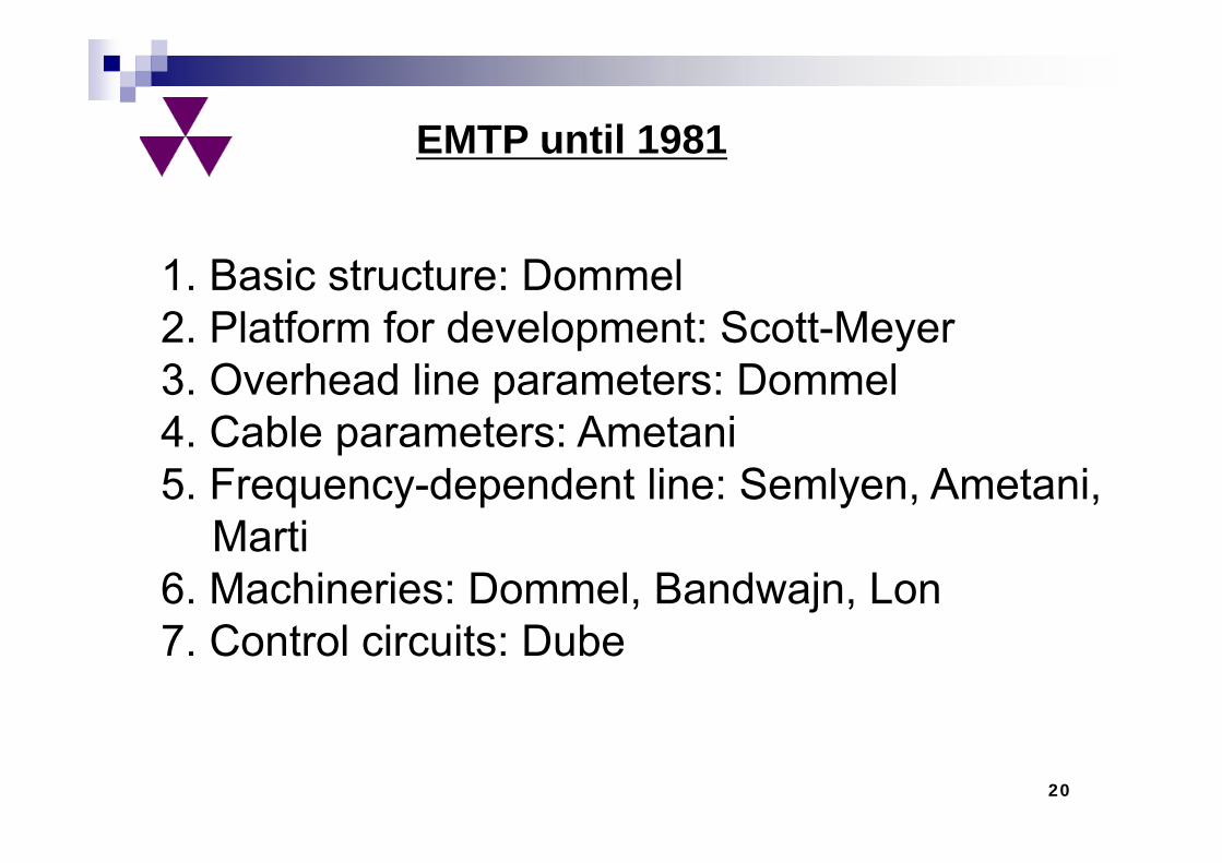
1. Basic structure: Dommel 2. Platform for development: Scott-Meyer3. Overhead line parameters: Dommel4. Cable parameters: Ametani5. Frequency-dependent line: Semlyen, Ametani,

Marti6. Machineries: Dommel, Bandwajn, Lon7. Control circuits: Dube

EMTP until 1981

20

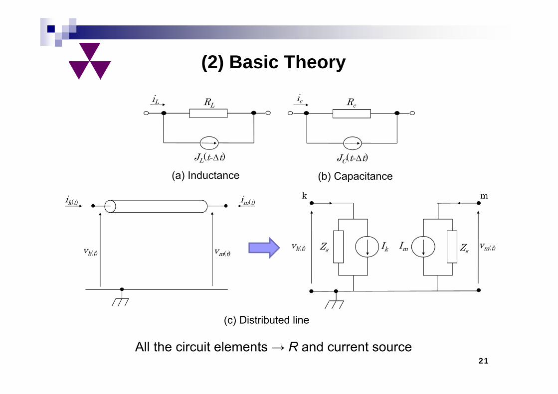
(2) Basic Theory

ik(t) im(t)

vk(t) vm(t)vk(t) vm(t)

k m

ZsZs Ik Im

(c) Distributed line

(a) Inductance (b) Capacitance

iciL RcRL

JL(t-∆t) JC(t-∆t)

All the circuit elements → R and current source21

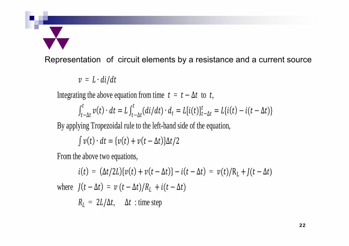
= ∙ / Integrating the above equation from time = ∆ to ,

∙ / ∙∆∆ ∆ ∆ By applying Tropezoidal rule to the left-hand side of the equation, ∙ ∆ ∆ /2 From the above two equations, = ∆ /2 ∆ ∆ = /RL ∆ )where ∆ = ∆ / ∆ = 2 /∆ , ∆ : time step

Representation of circuit elements by a resistance and a current source

22

1

I2

I3

I4

I5

I6

IA IB IC

R1R2

R3

R4

R5

R6

E1 E2 E6

1 2

3 4

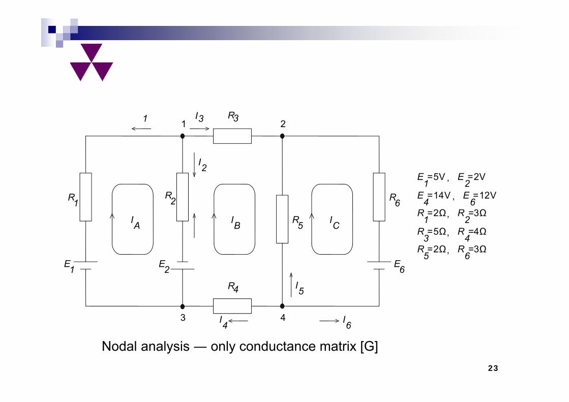
E1=5V，E

2=2V

E4=14V，E

6=12V

R1=2Ω，R

2=3Ω

R3=5Ω，R

4=4Ω

R5=2Ω，R

6=3Ω

Nodal analysis ― only conductance matrix [G]23

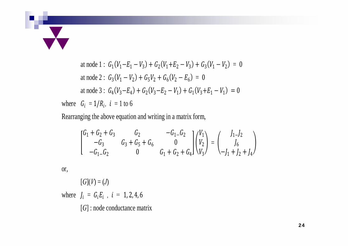
at node 1 : 1 1 1 3 2 1 2 3 3 1 2 = 0 at node 2 : 3 1 2 5 2 6 2 6 = 0 at node 3 : 4 3 4 2 3 2 1 1 3 1 1 0 where =1/ , = 1 to 6 Rearranging the above equation and writing in a matrix form,

1 2 3 2 1 2

3 3 5 6 01 2 0 1 2 4

123

= 1 26

1 2 4

or, [G](V) = (J) where = , = 1, 2, 4, 6 [G] : node conductance matrix

24

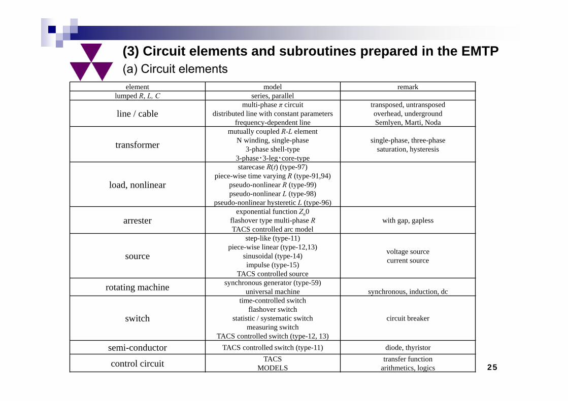
(3) Circuit elements and subroutines prepared in the EMTP(a) Circuit elementselement model remark

lumped R, L, C series, parallel

line / cablemulti-phase π circuit

distributed line with constant parametersfrequency-dependent line

transposed, untransposedoverhead, undergroundSemlyen, Marti, Noda

transformermutually coupled R-L element

N winding, single-phase3-phase shell-type

3-phase･3-leg･core-type

single-phase, three-phasesaturation, hysteresis

load, nonlinear

starecase R(t) (type-97)piece-wise time varying R (type-91,94)

pseudo-nonlinear R (type-99)pseudo-nonlinear L (type-98)

pseudo-nonlinear hysteretic L (type-96)

arresterexponential function Zn0

flashover type multi-phase RTACS controlled arc model

with gap, gapless

source

step-like (type-11)piece-wise linear (type-12,13)

sinusoidal (type-14)impulse (type-15)

TACS controlled source

voltage sourcecurrent source

rotating machine synchronous generator (type-59)universal machine synchronous, induction, dc

switch

time-controlled switchflashover switch

statistic / systematic switchmeasuring switch

TACS controlled switch (type-12, 13)

circuit breaker

semi-conductor TACS controlled switch (type-11) diode, thyristor

control circuit TACSMODELS

transfer functionarithmetics, logics 25

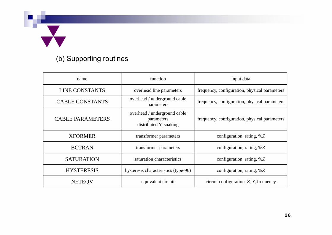
(b) Supporting routines

name function input data

LINE CONSTANTS overhead line parameters frequency, configuration, physical parameters

CABLE CONSTANTS overhead / underground cable parameters frequency, configuration, physical parameters

CABLE PARAMETERSoverhead / underground cable

parametersdistributed Y, snaking

frequency, configuration, physical parameters

XFORMER transformer parameters configuration, rating, %Z

BCTRAN transformer parameters configuration, rating, %Z

SATURATION saturation characteristics configuration, rating, %Z

HYSTERESIS hysteresis characteristics (type-96) configuration, rating, %Z

NETEQV equivalent circuit circuit configuration, Z, Y, frequency

26

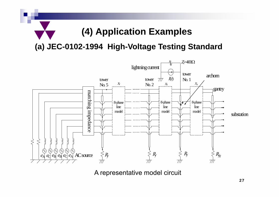
(a) JEC-0102-1994 High-Voltage Testing Standard

(4) Application Examples

A representative model circuit

substation

matching im

pedance

8-phaseline

model

tower No. 5 xt

eA eC eB eB eC eA Rf AC source

Zl=400

8-phaseline

model

8-phaseline

model

gantry

archorn tower No. 2

tower No. 1

xs

xt

Rf Rf Rfg

lightning current

I(t)

27

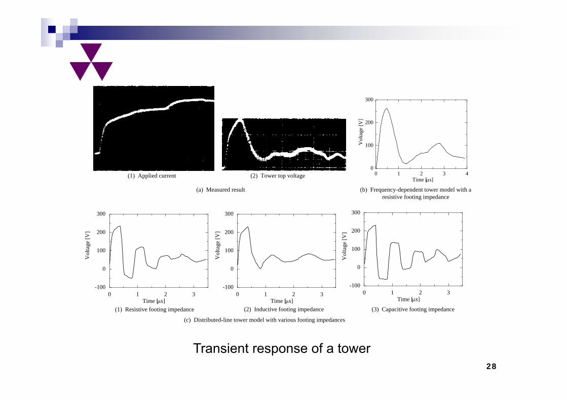
Transient response of a tower

(c) Distributed-line tower model with various footing impedances

(a) Measured result

(1) Applied current (2) Tower top voltage

(b) Frequency-dependent tower model with a resistive footing impedance

0 1 2 3 40

100

200

300

Time [s]

Vol

tage

[V]

0 1 2 3-100

0

100

200

300

Time [s]

Vol

tage

[V]

(1) Resistive footing impedance

0 1 2 3-100

0

100

200

300

Time [s]

Vol

tage

[V]

(2) Inductive footing impedance

0 1 2 3-100

0

100

200

300

Time [s]

Vol

tage

[V]

(3) Capacitive footing impedance

28

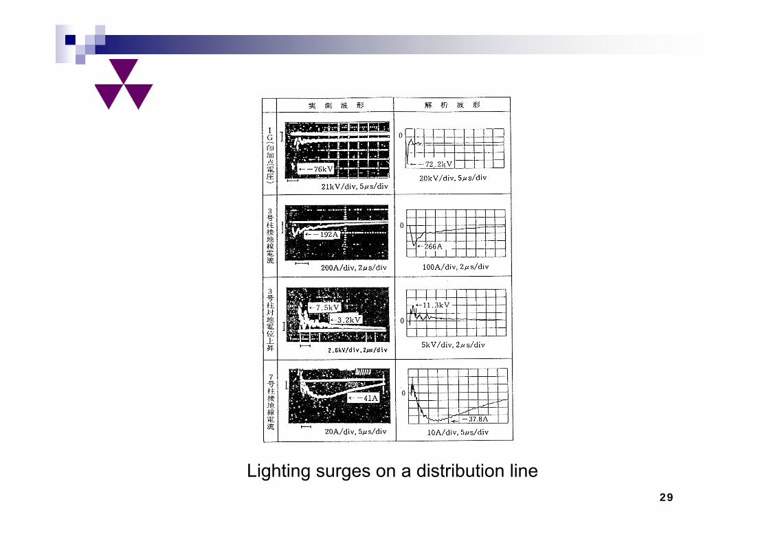
Lighting surges on a distribution line29

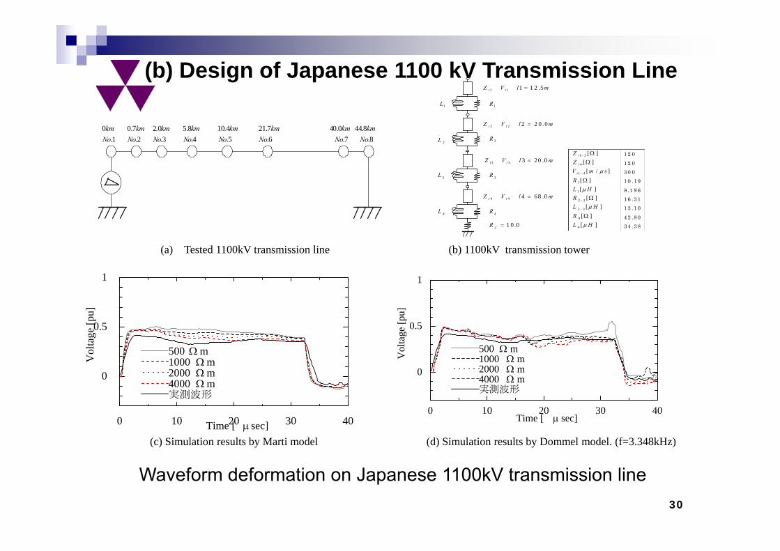
Waveform deformation on Japanese 1100kV transmission line

1.No 2.No 4.No3.No 5.No 6.No 7.No 8.Nokm0 km8.44km0.40km7.21km4.10km8.5km0.2km7.0

][31 tZ ][4 tZ

]/[41 smV t ][1 R

][1 HL ][32 R

][32 HL ][4 R

][4 HL

1 2 0 1 2 0 3 0 0 1 0 .1 98 .1 8 61 6 .3 11 3 .1 04 2 .8 03 4 .3 8

mlVZ tt 5.1 2111

mlVZ tt 0.68444

mlVZ tt 0.2 0222

mlVZ tt 0.20333

1L

2L

3L

4L

1R

2R

3R

4R

0.1 0fR

0 10 20 30 40

0

0.5

1

Time [ sec]

Vol

tage

[pu]

500 m1000 m2000 m4000 m実測波形

0 10 20 30 40

0

0.5

1

Time [ sec]

Vol

tage

[pu]

500 m1000 m2000 m4000 m実測波形

(a) Tested 1100kV transmission line (b) 1100kV transmission tower

(c) Simulation results by Marti model (d) Simulation results by Dommel model. (f=3.348kHz)

(b) Design of Japanese 1100 kV Transmission Line

30

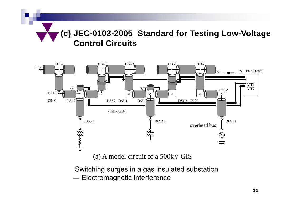
Switching surges in a gas insulated substation ― Electromagnetic interference

BUS3-1

DS3-2

VT2 VT1 VT2VT1

control cable

CB1-2 CB2-2CB2-1 CB3-1 CB3-2

DS1-1

DS1-M DS1-2 DS2-2 DS3-1

BUS2-1 BUS1-1

DS4-2 DS5-1

DS5-2

overhead bus

100m control roomBUS0

(a) A model circuit of a 500kV GIS

(c) JEC-0103-2005 Standard for Testing Low-Voltage Control Circuits

31

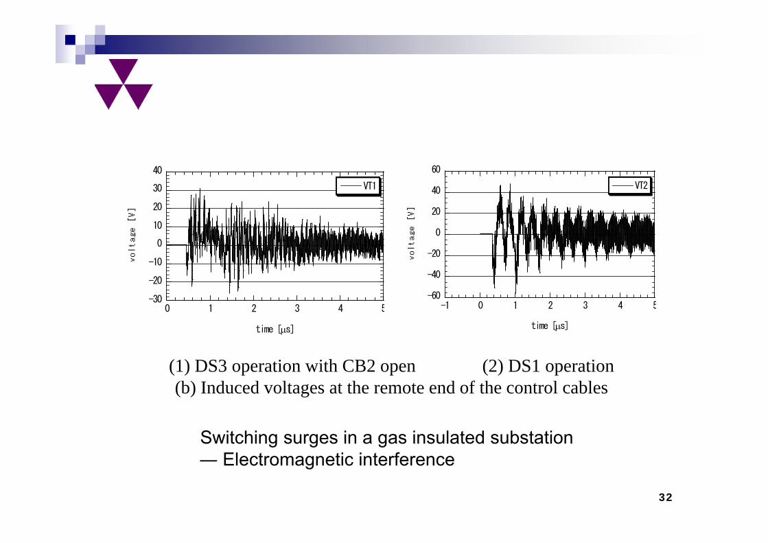
Switching surges in a gas insulated substation ― Electromagnetic interference

-30

-20

-10

0

10

20

30

40

0 1 2 3 4 5

VT1

time [s]

-60

-40

-20

0

20

40

60

-1 0 1 2 3 4 5

VT2

time [s]

(1) DS3 operation with CB2 open (2) DS1 operation(b) Induced voltages at the remote end of the control cables

32

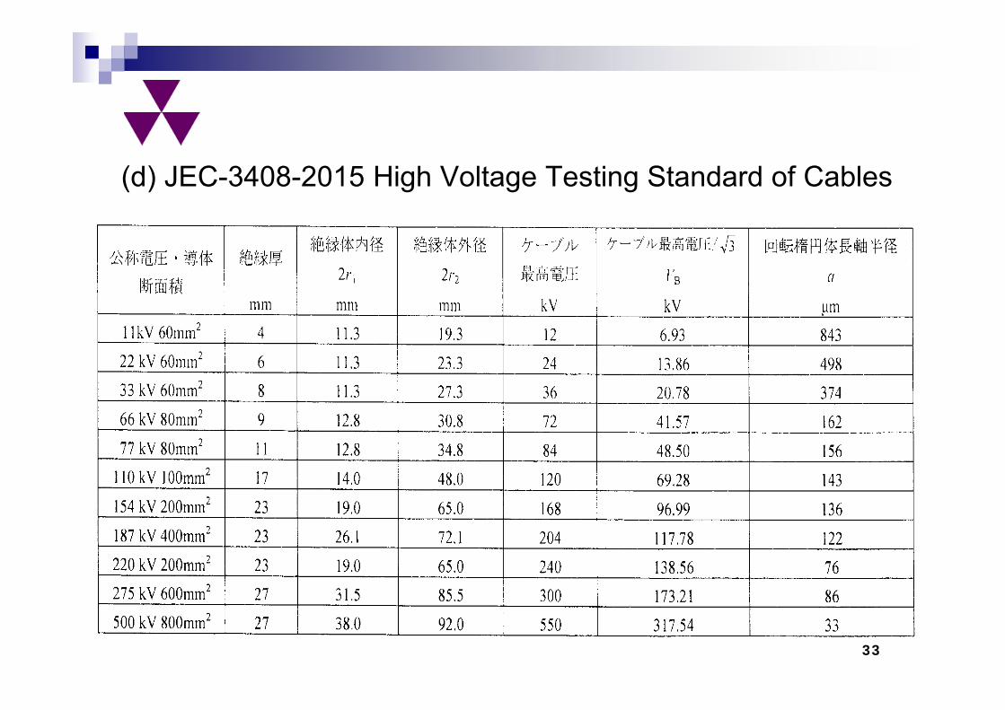
(d) JEC-3408-2015 High Voltage Testing Standard of Cables

33

(5) Application Limits / Problems

･ Any circuit – theory based approach is within TEM mode propagation of electromagnetic waves.

･ Impedance / Admittance formulas used in the approach assume :length x >> height h >> radius r .

･ Unknown parameters : earth resistivity along a line and depthfrequency / temperature – dependent permittivitystray capacitance / residual inductance of equipmentsemiconducting layer parameters

34

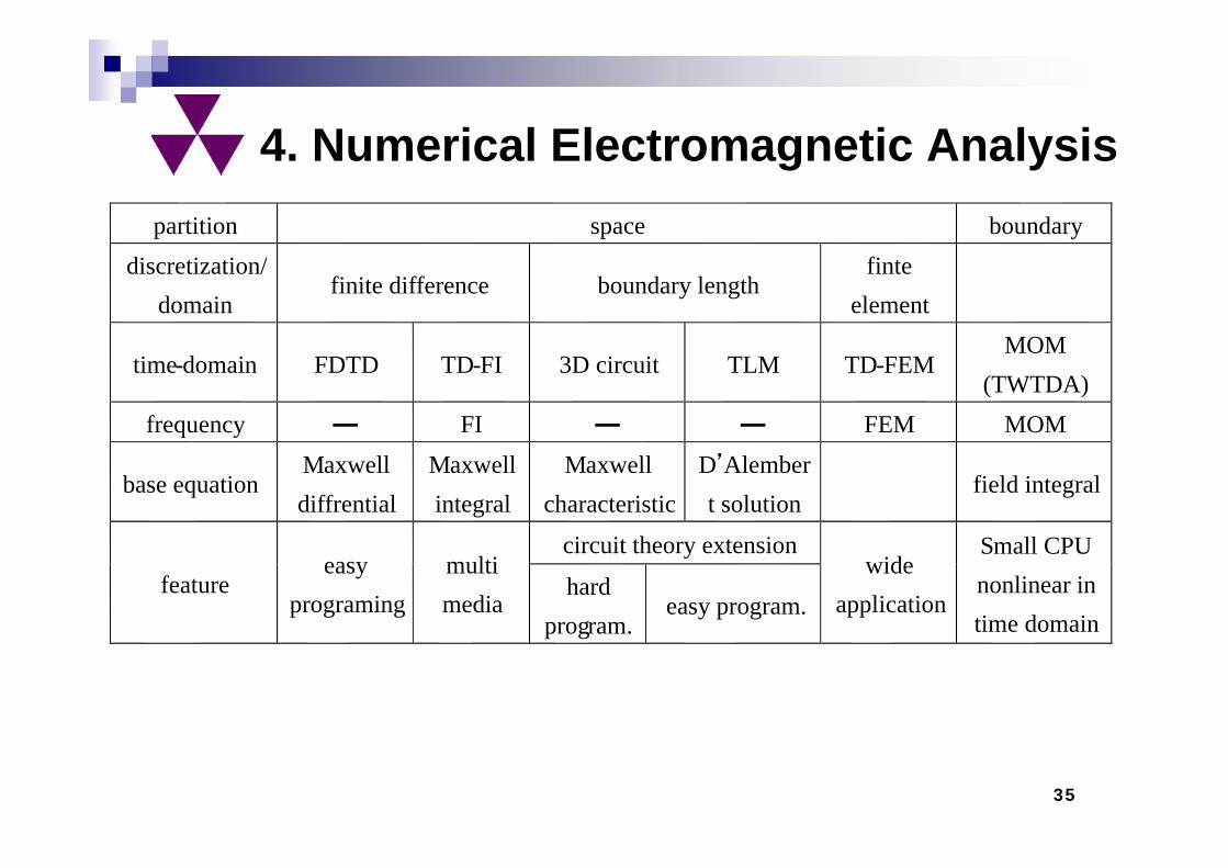
4. Numerical Electromagnetic Analysispartition space boundary

discretization/domain

finite difference boundary lengthfinte

element

time-domain FDTD TD-FI 3D circuit TLM TD-FEMMOM

(TWTDA)frequency FI FEM MOM

base equationMaxwell diffrential

Maxwell integral

Maxwell characteristic

D’Alembert solution

field integral

featureeasy

programingmulti media

circuit theory extensionwide

application

Small CPU nonlinear intime domain

hard program.

easy program.

35

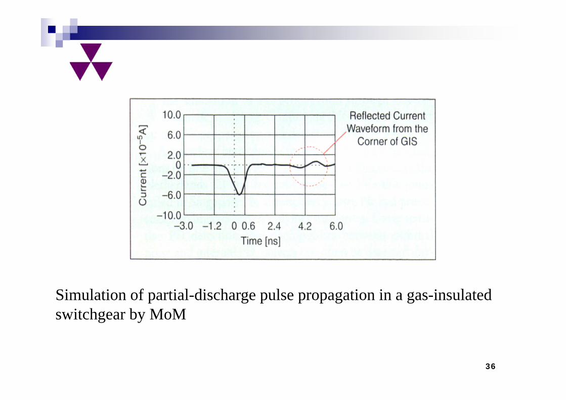
Simulation of partial-discharge pulse propagation in a gas-insulated switchgear by MoM

36

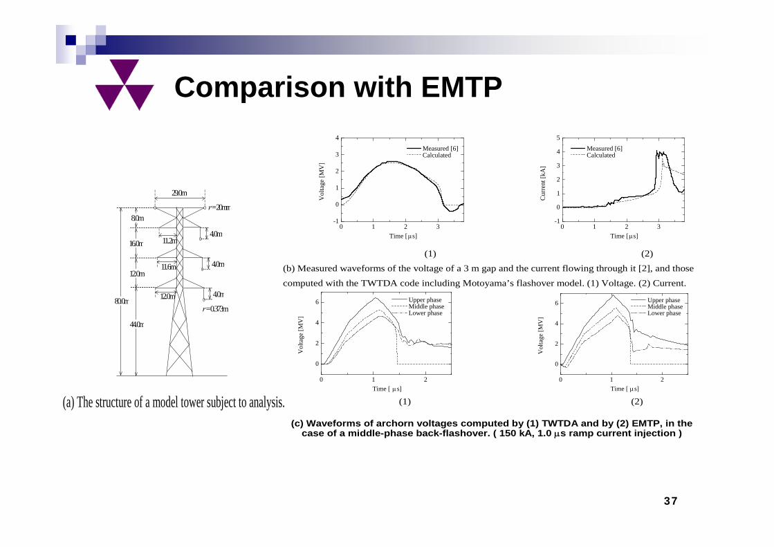
0 1 2 3-1

0

1

2

3

4

Time [s]

Vol

tage

[MV

]

Measured [6] Calculated

0 1 2 3

-1

0

1

2

3

4

5

Time [s]

Cur

rent

[kA

]

Measured [6] Calculated

(1) (2) (b) Measured waveforms of the voltage of a 3 m gap and the current flowing through it [2], and those computed with the TWTDA code including Motoyama’s flashover model. (1) Voltage. (2) Current.

0 1 2

0

2

4

6

Time [ s]

Vol

tage

[MV

] Upper phase Middle phase Lower phase

0 1 2

0

2

4

6

Time [ s]

Vol

tage

[MV

]

Upper phase Middle phase Lower phase

(1) (2)

(c) Waveforms of archorn voltages computed by (1) TWTDA and by (2) EMTP, in the case of a middle-phase back-flashover. ( 150 kA, 1.0 s ramp current injection )

29.0m

8.0m

16.0m

12.0m

44.0m

4.0m

4.0m

4.0m

11.2m

11.6m

12.0m

r = 20mm

80.0mr = 0.373m

(a) The structure of a model tower subject to analysis.

Comparison with EMTP

37

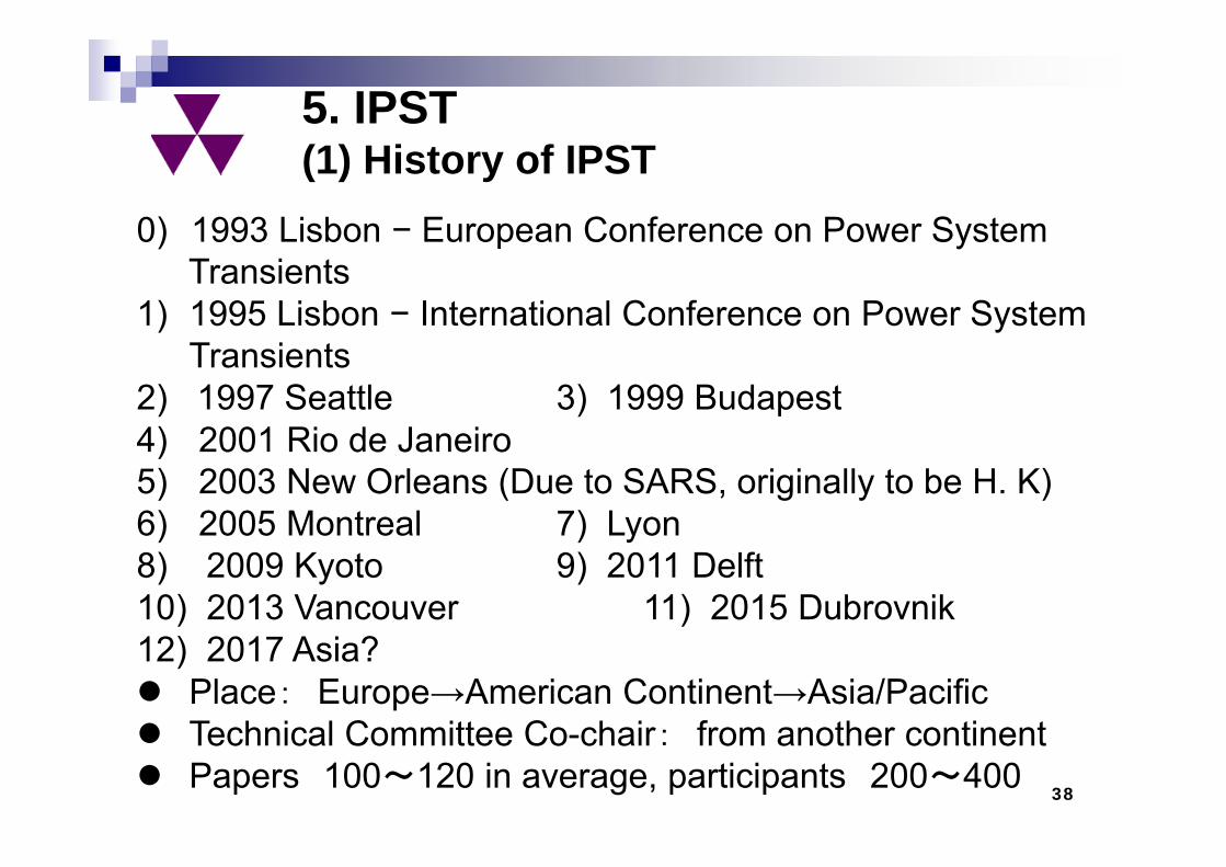
5. IPST(1) History of IPST

0) 1993 Lisbon − European Conference on Power System Transients

1) 1995 Lisbon − International Conference on Power System Transients

2) 1997 Seattle 3) 1999 Budapest4) 2001 Rio de Janeiro5) 2003 New Orleans (Due to SARS, originally to be H. K)6) 2005 Montreal 7) Lyon8) 2009 Kyoto 9) 2011 Delft10) 2013 Vancouver 11) 2015 Dubrovnik12) 2017 Asia? Place： Europe→American Continent→Asia/Pacific Technical Committee Co-chair： from another continent Papers 100～120 in average, participants 200～400

38

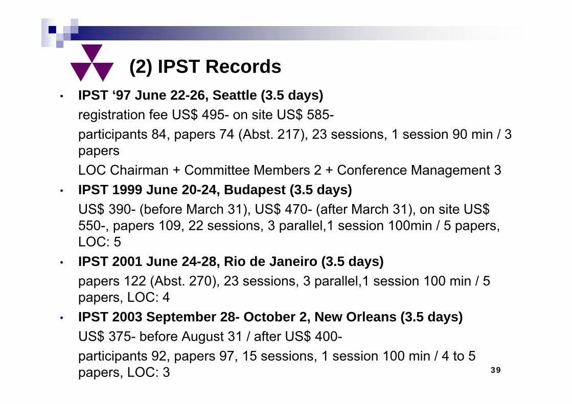
• IPST ‘97 June 22-26, Seattle (3.5 days)registration fee US$ 495- on site US$ 585-participants 84, papers 74 (Abst. 217), 23 sessions, 1 session 90 min / 3 papersLOC Chairman + Committee Members 2 + Conference Management 3

• IPST 1999 June 20-24, Budapest (3.5 days)US$ 390- (before March 31), US$ 470- (after March 31), on site US$ 550-, papers 109, 22 sessions, 3 parallel,1 session 100min / 5 papers, LOC: 5

• IPST 2001 June 24-28, Rio de Janeiro (3.5 days)papers 122 (Abst. 270), 23 sessions, 3 parallel,1 session 100 min / 5 papers, LOC: 4

• IPST 2003 September 28- October 2, New Orleans (3.5 days)US$ 375- before August 31 / after US$ 400-participants 92, papers 97, 15 sessions, 1 session 100 min / 4 to 5 papers, LOC: 3

(2) IPST Records

39

40

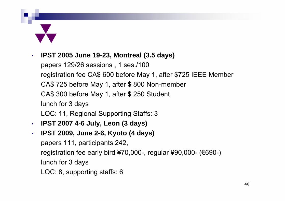
• IPST 2005 June 19-23, Montreal (3.5 days)papers 129/26 sessions , 1 ses./100 registration fee CA$ 600 before May 1, after $725 IEEE MemberCA$ 725 before May 1, after $ 800 Non-memberCA$ 300 before May 1, after $ 250 Studentlunch for 3 daysLOC: 11, Regional Supporting Staffs: 3

• IPST 2007 4-6 July, Leon (3 days)• IPST 2009, June 2-6, Kyoto (4 days)

papers 111, participants 242, registration fee early bird ¥70,000-, regular ¥90,000- (€690-)lunch for 3 daysLOC: 8, supporting staffs: 6

41

a) IPST expands intoPower systems, stability, controlRelaying, fault locationPower Electronics

b) Real-time simulatorsApplication vs developmentHardware in the loop testing

c) Integration of various tools: MatLab, FEMd) Numerical Electromagnetic Analysis

(3) Trends