IP2:*Image*Processing*in*Remote*Sensing* 7.SensorsII ...seppke/content/teaching... · Agenda, •...
43
MINFakultät Fachbereich Informa7k Arbeitsbereich SAV/BV (KOGS) IP2: Image Processing in Remote Sensing 7. Sensors II: Microwave Sensors and SAR Systems Summer Semester 2014 Benjamin Seppke
Transcript of IP2:*Image*Processing*in*Remote*Sensing* 7.SensorsII ...seppke/content/teaching... · Agenda, •...
MIN-‐Fakultät Fachbereich Informa7k Arbeitsbereich SAV/BV (KOGS)
IP2: Image Processing in Remote Sensing 7. Sensors II:
Microwave Sensors and SAR Systems Summer Semester 2014
Benjamin Seppke
Agenda
• General Microwave Sensors – Passive Systems – AcJve Systems
• AlJmeter • ScaKerometer
• SAR-‐Sensors – Design – From Low-‐ to High-‐ResoluJon Systems – Challenges for Image Processing
• Other Sensors
19.06.14 Benjamin Seppke, IP2: Remote Sensing, University of Hamburg, Dept. InformaJcs 2
Lecture 7: Sensors II – Microwave Sensors and SAR Systems
Microwave Systems
• Strong differences in Imaging compared to former (visible light and infrared) sensors!
• Nearly no interference when passing the atmosphere and some atmospheric phenomena: – Clouds – Dust – Smoke – Snow – Light rain
• Allows (nearly) weather independent observaJon • Wavelengths are between 1 mm – 1 m, which
corresponds to 300 GHz – 300 MHz 19.06.14 Benjamin Seppke, IP2: Remote Sensing, University of Hamburg, Dept. InformaJcs 3
Lecture 7: Sensors II – Microwave Sensors and SAR Systems
Passive Microwave Sensors • (Main) emit of the earth at microwave wavelengths: material
temperature • Signals at these spectral ranges may contain informaJon
about – Snow coverage – Soil moisture – Soil composiJon
• But: Signals are of low intensity! Low geometric resoluJon (mainly Push Broom Scanners) No SynopJcal image generaJon
• High construcJon efforts to enhance signal to noise raJo (SNR)
19.06.14 Benjamin Seppke, IP2: Remote Sensing, University of Hamburg, Dept. InformaJcs 4
Lecture 7: Sensors II – Microwave Sensors and SAR Systems
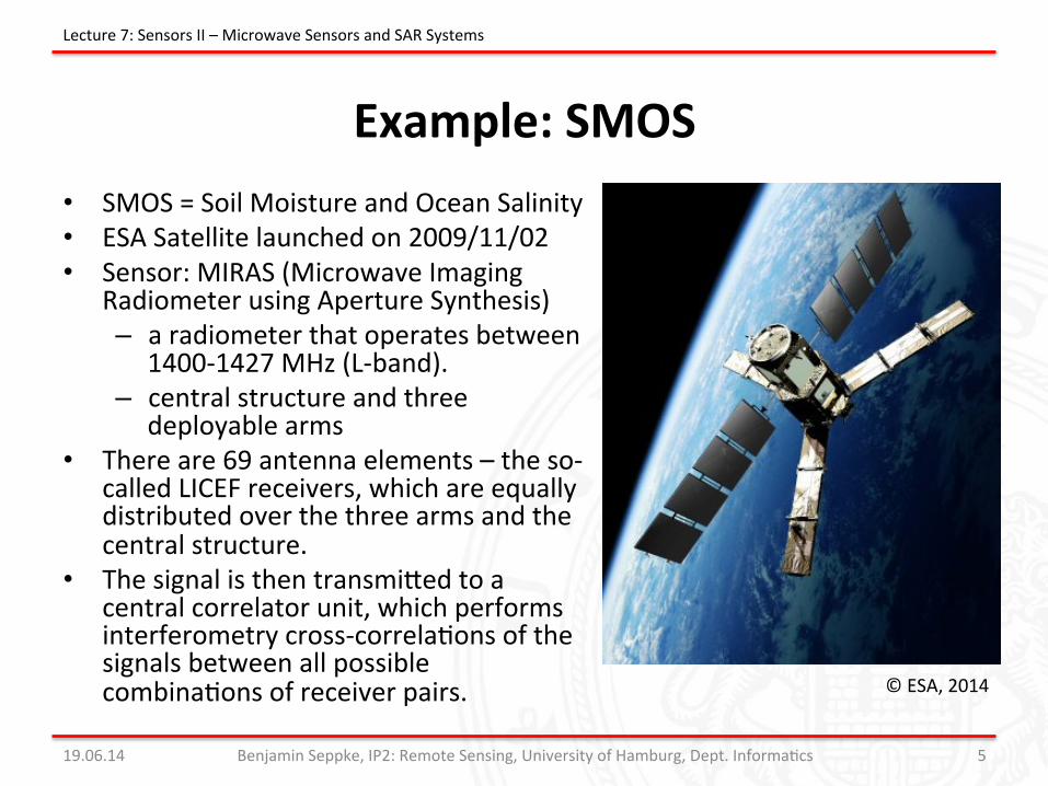
Example: SMOS • SMOS = Soil Moisture and Ocean Salinity • ESA Satellite launched on 2009/11/02 • Sensor: MIRAS (Microwave Imaging
Radiometer using Aperture Synthesis) – a radiometer that operates between
1400-‐1427 MHz (L-‐band). – central structure and three
deployable arms • There are 69 antenna elements – the so-‐
called LICEF receivers, which are equally distributed over the three arms and the central structure.
• The signal is then transmiKed to a central correlator unit, which performs interferometry cross-‐correlaJons of the signals between all possible combinaJons of receiver pairs.
19.06.14 Benjamin Seppke, IP2: Remote Sensing, University of Hamburg, Dept. InformaJcs 5
Lecture 7: Sensors II – Microwave Sensors and SAR Systems
© ESA, 2014
SMOS Satellite: ESA’s Water Mission hKp://www.youtube.com/watch?v=Kw0umICWXuU
19.06.14 Benjamin Seppke, IP2: Remote Sensing, University of Hamburg, Dept. InformaJcs 6
Lecture 7: Sensors II – Microwave Sensors and SAR Systems
Ac7ve Microwave Systems • CategorizaJon:
– Real vs. SyntheJc Aperture Radar (SAR) – Push broom vs. Side looking – Single vs. MulJ/Cross-‐PolarizaJon – Single vs. MulJ-‐Band Systems
• AcJve Systems! – Formerly high energy consumpJon -‐> addiJonal baKeries needed
– Nowadays: Solar panel power sufficient! • Different bands for different observaJons • Not every configuraJon available:
– currently not mulJ-‐band SAR in orbit – some systems allow cross-‐ or single polarizaJon
19.06.14 Benjamin Seppke, IP2: Remote Sensing, University of Hamburg, Dept. InformaJcs 7
Lecture 7: Sensors II – Microwave Sensors and SAR Systems
Satellite based Al7metry • Typical applicaJons:
– Earth surface height – Ocean water level/distribuJon (important climate parameter)
• Push broom/point wise measurements • System design – down-‐facing:
1. Emit Microwaves of certain power 2. Measure backscaKered energy and runJme 3. Derive AlJmetry from measured data
• Note: – Measured alJtude needs to be normalized w.r.t the earths geoid
(gravity distribuJon is non-‐uniform) – IFOV (Footprint) size/resoluJon depends on aperture size of the
antenna – Typical Sensors achieve low spaJal but high measurement precision!
19.06.14 Benjamin Seppke, IP2: Remote Sensing, University of Hamburg, Dept. InformaJcs 8
Lecture 7: Sensors II – Microwave Sensors and SAR Systems
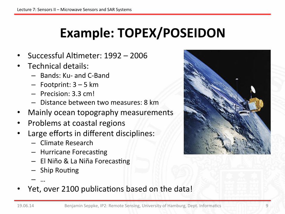
Example: TOPEX/POSEIDON • Successful AlJmeter: 1992 – 2006 • Technical details:
– Bands: Ku-‐ and C-‐Band – Footprint: 3 – 5 km – Precision: 3.3 cm! – Distance between two measures: 8 km
• Mainly ocean topography measurements • Problems at coastal regions • Large efforts in different disciplines:
– Climate Research – Hurricane ForecasJng – El Niño & La Niña ForecasJng – Ship RouJng – …
• Yet, over 2100 publicaJons based on the data!
19.06.14 Benjamin Seppke, IP2: Remote Sensing, University of Hamburg, Dept. InformaJcs 9
Lecture 7: Sensors II – Microwave Sensors and SAR Systems
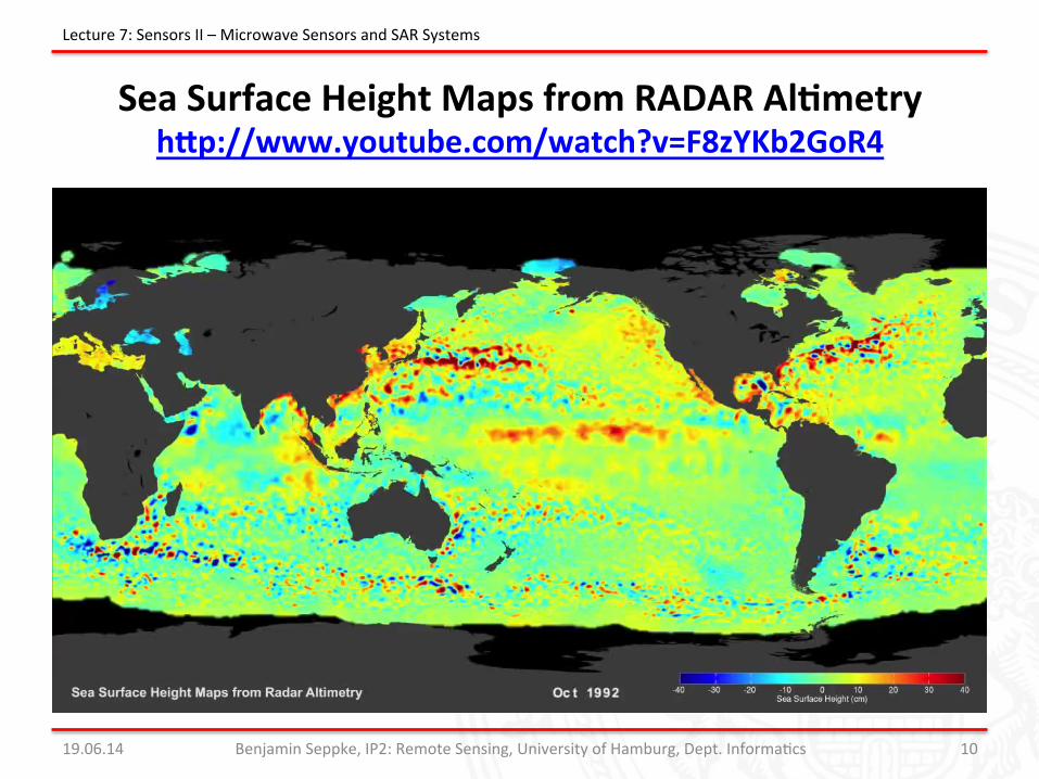
Sea Surface Height Maps from RADAR Al7metry hKp://www.youtube.com/watch?v=F8zYKb2GoR4
19.06.14 Benjamin Seppke, IP2: Remote Sensing, University of Hamburg, Dept. InformaJcs 10
Lecture 7: Sensors II – Microwave Sensors and SAR Systems
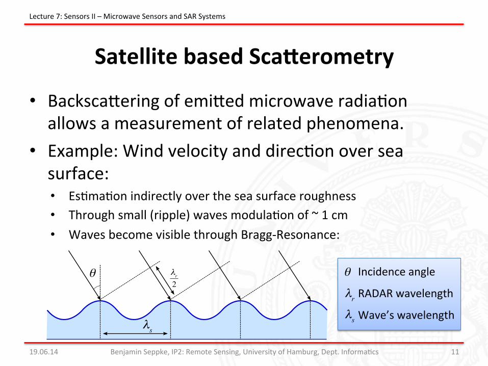
Satellite based ScaKerometry
• BackscaKering of emiKed microwave radiaJon allows a measurement of related phenomena.
• Example: Wind velocity and direcJon over sea surface: • EsJmaJon indirectly over the sea surface roughness • Through small (ripple) waves modulaJon of ~ 1 cm • Waves become visible through Bragg-‐Resonance:
19.06.14 Benjamin Seppke, IP2: Remote Sensing, University of Hamburg, Dept. InformaJcs 11
Lecture 7: Sensors II – Microwave Sensors and SAR Systems
θ
λs
λr2
θ
λrλs
Incidence angle
RADAR wavelength
Wave’s wavelength
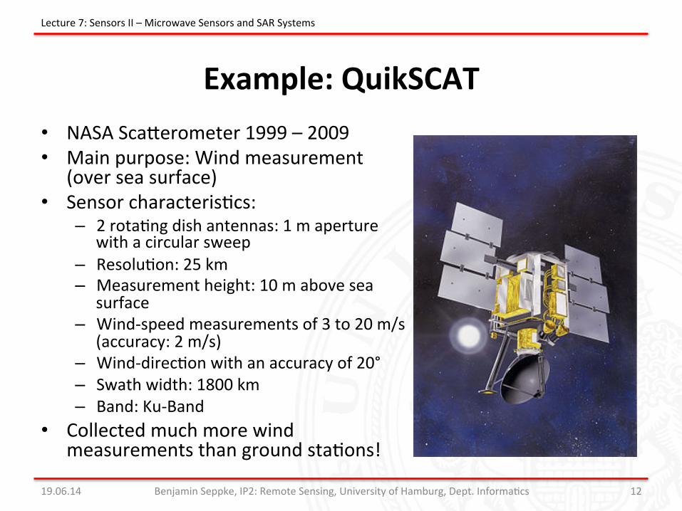
Example: QuikSCAT • NASA ScaKerometer 1999 – 2009 • Main purpose: Wind measurement
(over sea surface) • Sensor characterisJcs:
– 2 rotaJng dish antennas: 1 m aperture with a circular sweep
– ResoluJon: 25 km – Measurement height: 10 m above sea
surface – Wind-‐speed measurements of 3 to 20 m/s
(accuracy: 2 m/s) – Wind-‐direcJon with an accuracy of 20° – Swath width: 1800 km – Band: Ku-‐Band
• Collected much more wind measurements than ground staJons!
19.06.14 Benjamin Seppke, IP2: Remote Sensing, University of Hamburg, Dept. InformaJcs 12
Lecture 7: Sensors II – Microwave Sensors and SAR Systems
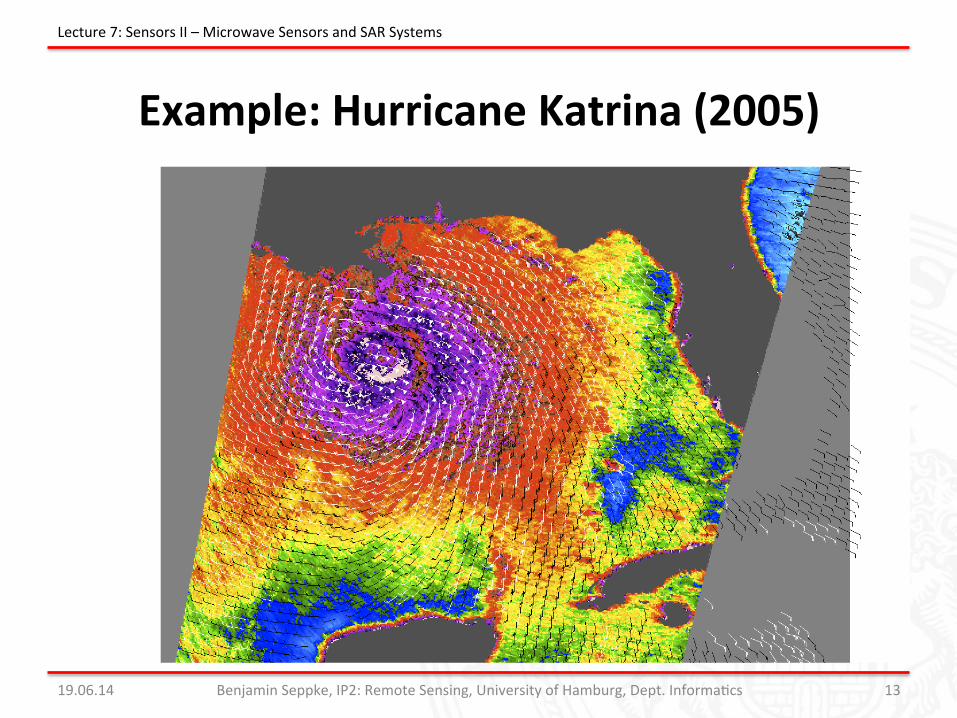
Example: Hurricane Katrina (2005)
19.06.14 Benjamin Seppke, IP2: Remote Sensing, University of Hamburg, Dept. InformaJcs 13
Lecture 7: Sensors II – Microwave Sensors and SAR Systems
RADAR vs. Photometric Resolu7on
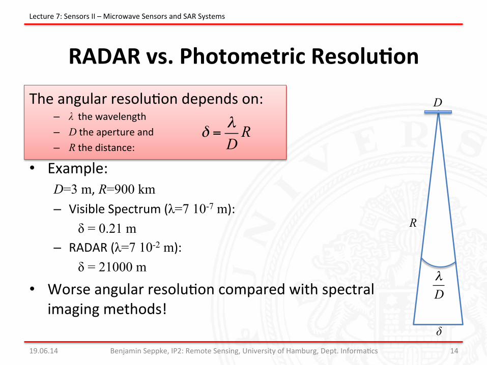
The angular resoluJon depends on: – λ the wavelength – D the aperture and – R the distance:
• Example: D=3 m, R=900 km – Visible Spectrum (λ=7 10-7 m):
δ = 0.21 m – RADAR (λ=7 10-2 m):
δ = 21000 m
• Worse angular resoluJon compared with spectral imaging methods! 19.06.14 Benjamin Seppke, IP2: Remote Sensing, University of Hamburg, Dept. InformaJcs 14
Lecture 7: Sensors II – Microwave Sensors and SAR Systems
δ =λDR
D
R
δ
λD
θ
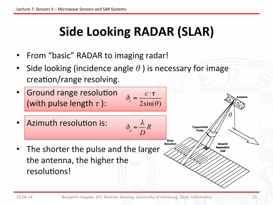
Side Looking RADAR (SLAR)
• From “basic” RADAR to imaging radar! • Side looking (incidence angle θ ) is necessary for image
creaJon/range resolving. • Ground range resoluJon
(with pulse length τ ):
• Azimuth resoluJon is:
• The shorter the pulse and the larger the antenna, the higher the resoluJons!
19.06.14 Benjamin Seppke, IP2: Remote Sensing, University of Hamburg, Dept. InformaJcs 15
Lecture 7: Sensors II – Microwave Sensors and SAR Systems
δr =c ⋅τ2sin(θ )
δa =λDR
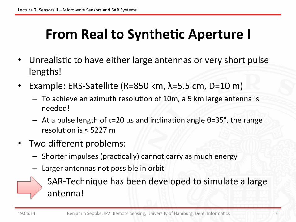
From Real to Synthe7c Aperture I
• UnrealisJc to have either large antennas or very short pulse lengths!
• Example: ERS-‐Satellite (R=850 km, λ=5.5 cm, D=10 m) – To achieve an azimuth resoluJon of 10m, a 5 km large antenna is
needed! – At a pulse length of τ=20 μs and inclinaJon angle θ=35°, the range
resoluJon is ≈ 5227 m
• Two different problems: – Shorter impulses (pracJcally) cannot carry as much energy – Larger antennas not possible in orbit SAR-‐Technique has been developed to simulate a large antenna!
19.06.14 Benjamin Seppke, IP2: Remote Sensing, University of Hamburg, Dept. InformaJcs 16
Lecture 7: Sensors II – Microwave Sensors and SAR Systems
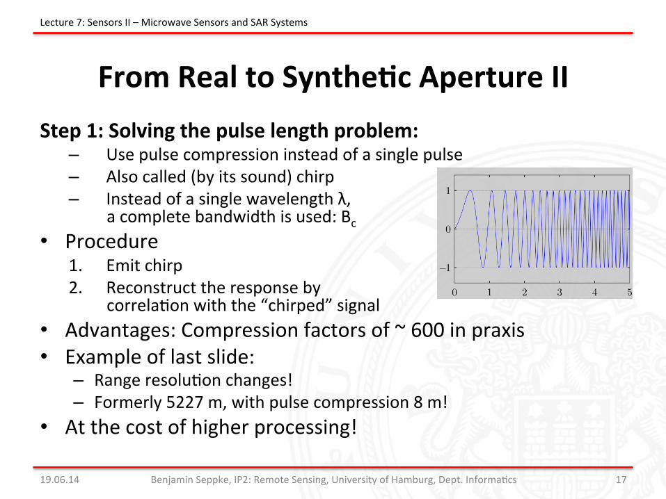
From Real to Synthe7c Aperture II Step 1: Solving the pulse length problem:
– Use pulse compression instead of a single pulse – Also called (by its sound) chirp – Instead of a single wavelength λ,
a complete bandwidth is used: Bc • Procedure
1. Emit chirp 2. Reconstruct the response by
correlaJon with the “chirped” signal • Advantages: Compression factors of ~ 600 in praxis • Example of last slide:
– Range resoluJon changes! – Formerly 5227 m, with pulse compression 8 m!
• At the cost of higher processing!
19.06.14 Benjamin Seppke, IP2: Remote Sensing, University of Hamburg, Dept. InformaJcs 17
Lecture 7: Sensors II – Microwave Sensors and SAR Systems
From Real to Synthe7c Aperture III
Step 2: Enhancing the azimuth resolu7on: • Idea: Make the RADAR system work coherently. Knowledge needed about phase shizs between – sender and receiver and – pulse to pulse
• Repeat measurements along-‐track and “synthesize” the short antennas to a large antenna!
• SAR synthesis step requirements – exact knowledge of posiJon and – exact orientaJon of the sender.
19.06.14 Benjamin Seppke, IP2: Remote Sensing, University of Hamburg, Dept. InformaJcs 18
Lecture 7: Sensors II – Microwave Sensors and SAR Systems
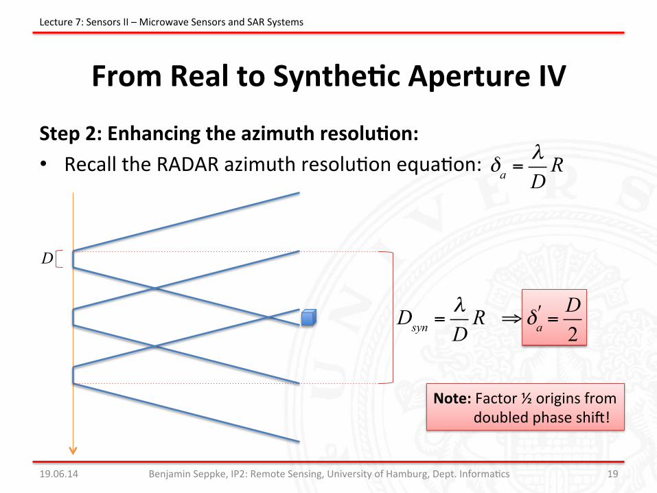
From Real to Synthe7c Aperture IV
Step 2: Enhancing the azimuth resolu7on: • Recall the RADAR azimuth resoluJon equaJon:
19.06.14 Benjamin Seppke, IP2: Remote Sensing, University of Hamburg, Dept. InformaJcs 19
Lecture 7: Sensors II – Microwave Sensors and SAR Systems
δa =λDR
D
Dsyn =λDR ⇒ δa" =
D2
Note: Factor ½ origins from doubled phase shiz!
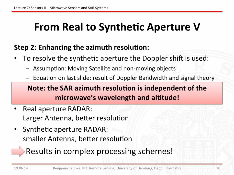
From Real to Synthe7c Aperture V
Step 2: Enhancing the azimuth resolu7on: • To resolve the syntheJc aperture the Doppler shiz is used:
– AssumpJon: Moving Satellite and non-‐moving objects – EquaJon on last slide: result of Doppler Bandwidth and signal theory Note: the SAR azimuth resolu7on is independent of the
microwave’s wavelength and al7tude! • Real aperture RADAR:
Larger Antenna, beKer resoluJon • SyntheJc aperture RADAR:
smaller Antenna, beKer resoluJon
Results in complex processing schemes!
19.06.14 Benjamin Seppke, IP2: Remote Sensing, University of Hamburg, Dept. InformaJcs 20
Lecture 7: Sensors II – Microwave Sensors and SAR Systems
Proper7es of Synthe7c Aperture RADAR (SAR) Systems
• Remember: Microwave Imaging ≠ Photometric Imaging! • Classical Radar: Target vs. CluKer • SAR: No equivalent to cluKer but point and area objects à
normalized backscaKer coefficient σ0 • MulJple scaKering/reflecJon of microwaves • Direct backscaKering on metal/arJficial objects • Length distorJon in range direcJon • SAR: Coherent Imaging à Coherent pixel value assignment
à Speckle “Noise”
19.06.14 Benjamin Seppke, IP2: Remote Sensing, University of Hamburg, Dept. InformaJcs 21
Lecture 7: Sensors II – Microwave Sensors and SAR Systems
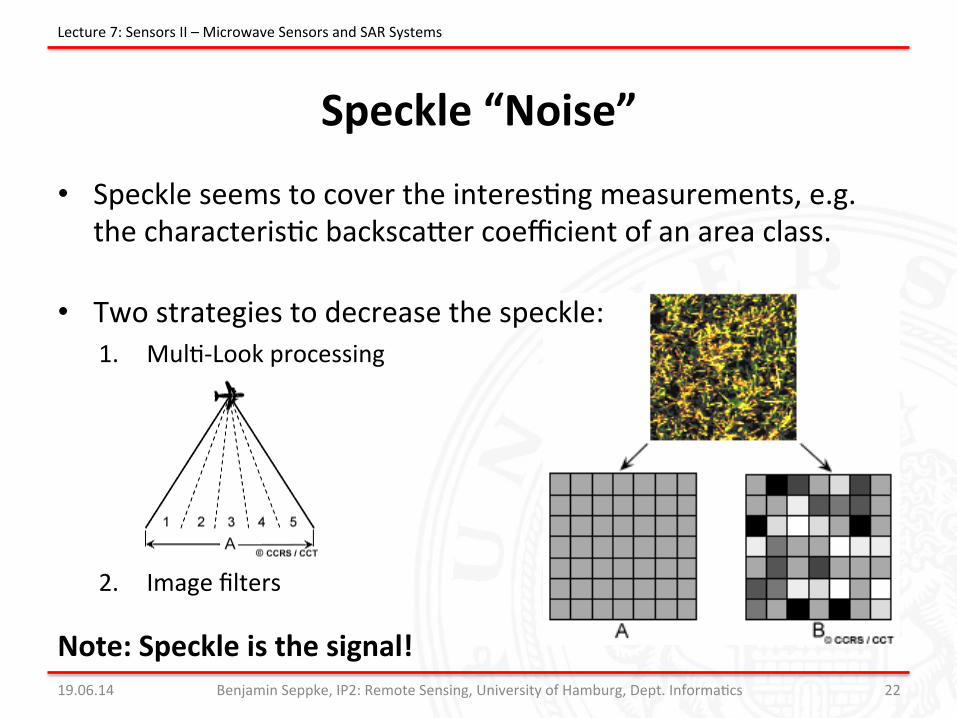
Speckle “Noise”
• Speckle seems to cover the interesJng measurements, e.g. the characterisJc backscaKer coefficient of an area class.
• Two strategies to decrease the speckle: 1. MulJ-‐Look processing
2. Image filters
Note: Speckle is the signal! 19.06.14 Benjamin Seppke, IP2: Remote Sensing, University of Hamburg, Dept. InformaJcs 22
Lecture 7: Sensors II – Microwave Sensors and SAR Systems
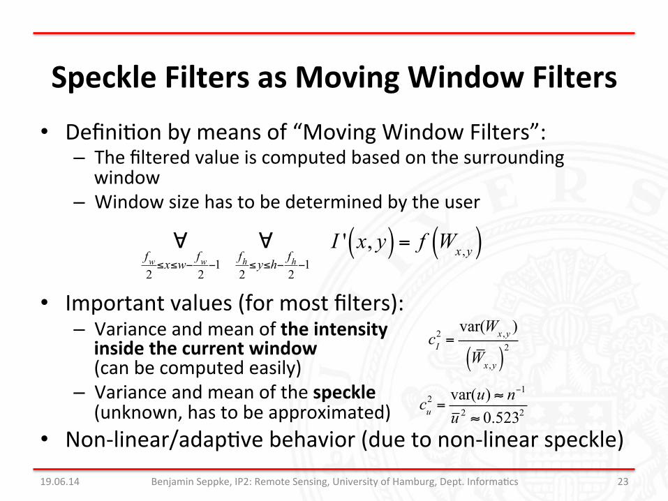
Speckle Filters as Moving Window Filters • DefiniJon by means of “Moving Window Filters”:
– The filtered value is computed based on the surrounding window
– Window size has to be determined by the user
• Important values (for most filters): – Variance and mean of the intensity inside the current window (can be computed easily)
– Variance and mean of the speckle (unknown, has to be approximated)
• Non-‐linear/adapJve behavior (due to non-‐linear speckle) 19.06.14 Benjamin Seppke, IP2: Remote Sensing, University of Hamburg, Dept. InformaJcs 23
∀fw2≤x≤w−
fw2−1
∀fh2≤y≤h−
fh2−1I ' x, y( ) = f Wx ,y( )
cu2 =var(u) ≈ n−1
u 2 ≈ 0.5232
cI2 =var(Wx ,y )
Wx ,y( )2
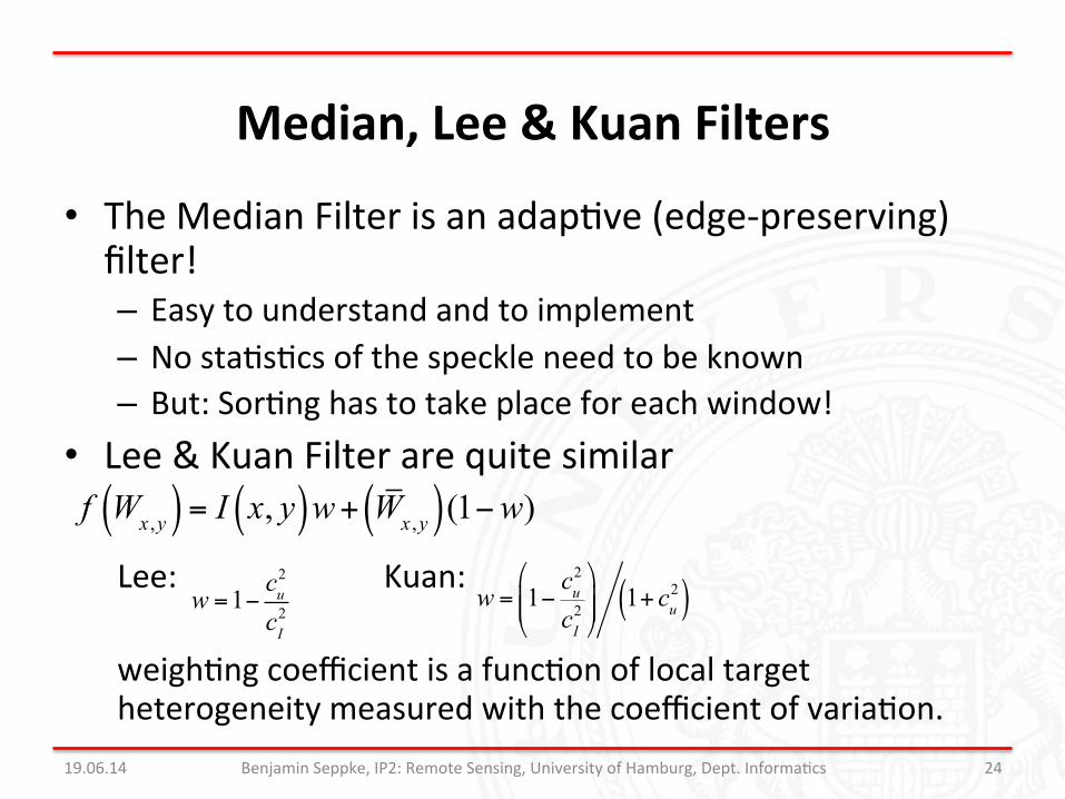
Median, Lee & Kuan Filters
• The Median Filter is an adapJve (edge-‐preserving) filter! – Easy to understand and to implement – No staJsJcs of the speckle need to be known – But: SorJng has to take place for each window!
• Lee & Kuan Filter are quite similar
Lee: Kuan: weighJng coefficient is a funcJon of local target heterogeneity measured with the coefficient of variaJon.
19.06.14 Benjamin Seppke, IP2: Remote Sensing, University of Hamburg, Dept. InformaJcs 24
f Wx ,y( ) = I x, y( )w+ Wx ,y( )(1−w)
w =1− cu2
cI2
w = 1− cu2
cI2
!
"##
$
%&& 1+ cu
2( )
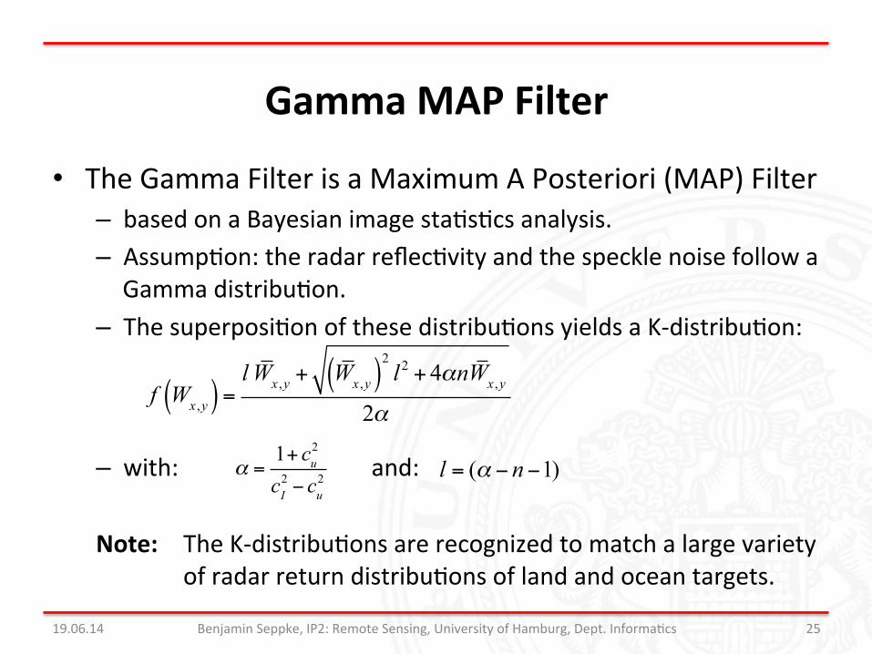
Gamma MAP Filter
• The Gamma Filter is a Maximum A Posteriori (MAP) Filter – based on a Bayesian image staJsJcs analysis. – AssumpJon: the radar reflecJvity and the speckle noise follow a Gamma distribuJon.
– The superposiJon of these distribuJons yields a K-‐distribuJon:
– with: and:
Note: The K-‐distribuJons are recognized to match a large variety of radar return distribuJons of land and ocean targets.
19.06.14 Benjamin Seppke, IP2: Remote Sensing, University of Hamburg, Dept. InformaJcs 25
f Wx ,y( ) =l Wx ,y + Wx ,y( )
2l2 + 4αnWx ,y
2α
α =1+ cu
2
cI2 − cu
2 l = (α − n−1)
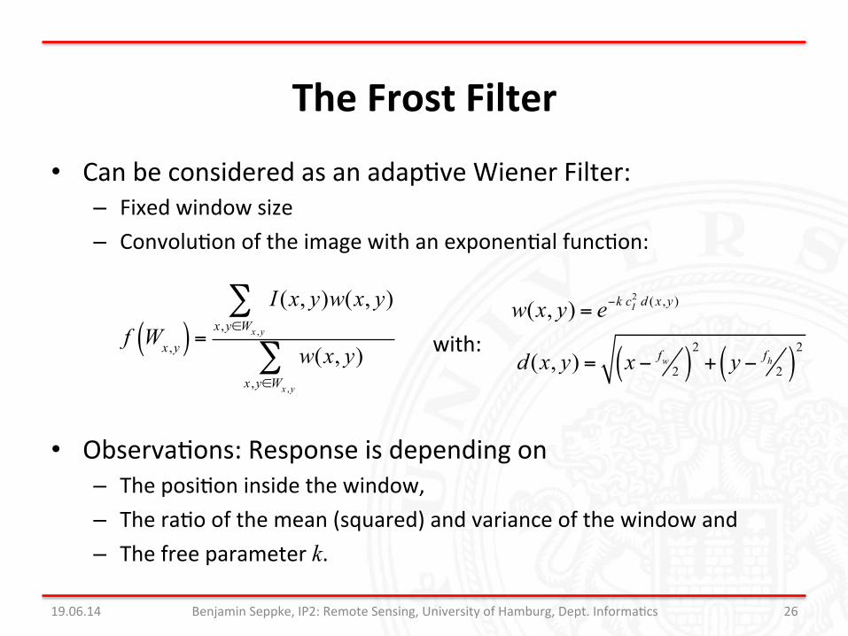
The Frost Filter
• Can be considered as an adapJve Wiener Filter: – Fixed window size – ConvoluJon of the image with an exponenJal funcJon:
with:
• ObservaJons: Response is depending on – The posiJon inside the window, – The raJo of the mean (squared) and variance of the window and – The free parameter k.
19.06.14 Benjamin Seppke, IP2: Remote Sensing, University of Hamburg, Dept. InformaJcs 26
f Wx ,y( ) =I (x, y)w(x, y)
x ,y∈Wx ,y
∑
w(x, y)x ,y∈Wx ,y
∑
w(x, y) = e−k cI2 d (x ,y )
d(x, y) = x − fw2( )2+ y − fh
2( )2
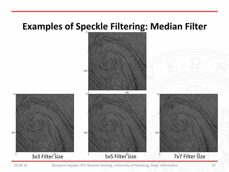
Examples of Speckle Filtering: Median Filter
19.06.14 Benjamin Seppke, IP2: Remote Sensing, University of Hamburg, Dept. InformaJcs 27
3x3 Filter size 5x5 Filter size 7x7 Filter size
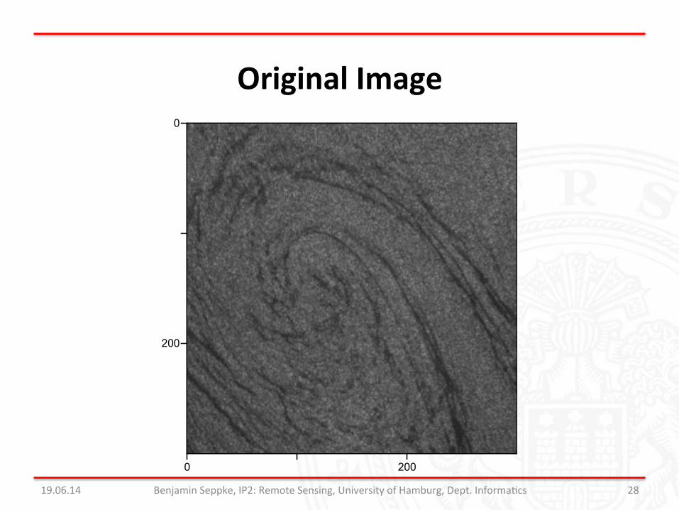
Original Image
19.06.14 Benjamin Seppke, IP2: Remote Sensing, University of Hamburg, Dept. InformaJcs 28

Median Filter (Filter size: 5x5)
19.06.14 Benjamin Seppke, IP2: Remote Sensing, University of Hamburg, Dept. InformaJcs 29
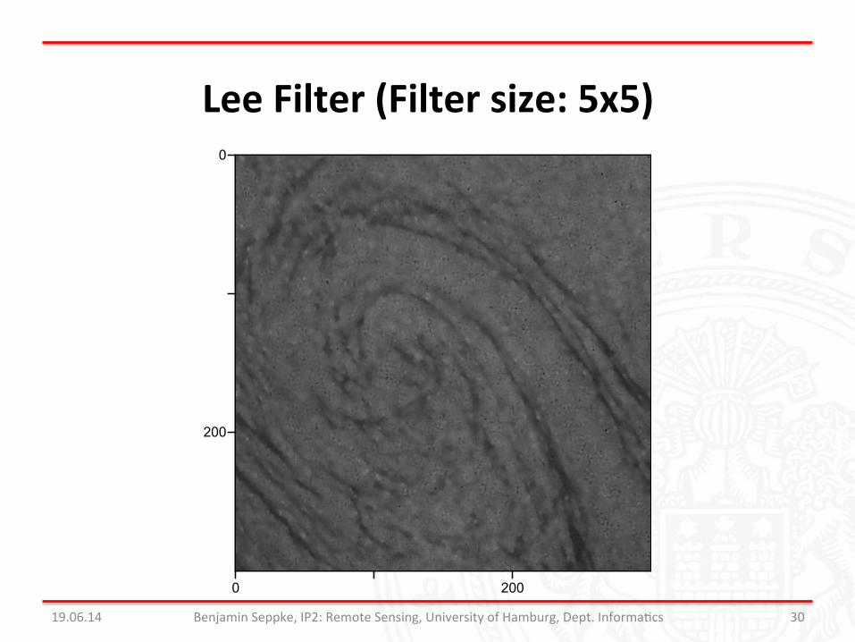
Lee Filter (Filter size: 5x5)
19.06.14 Benjamin Seppke, IP2: Remote Sensing, University of Hamburg, Dept. InformaJcs 30
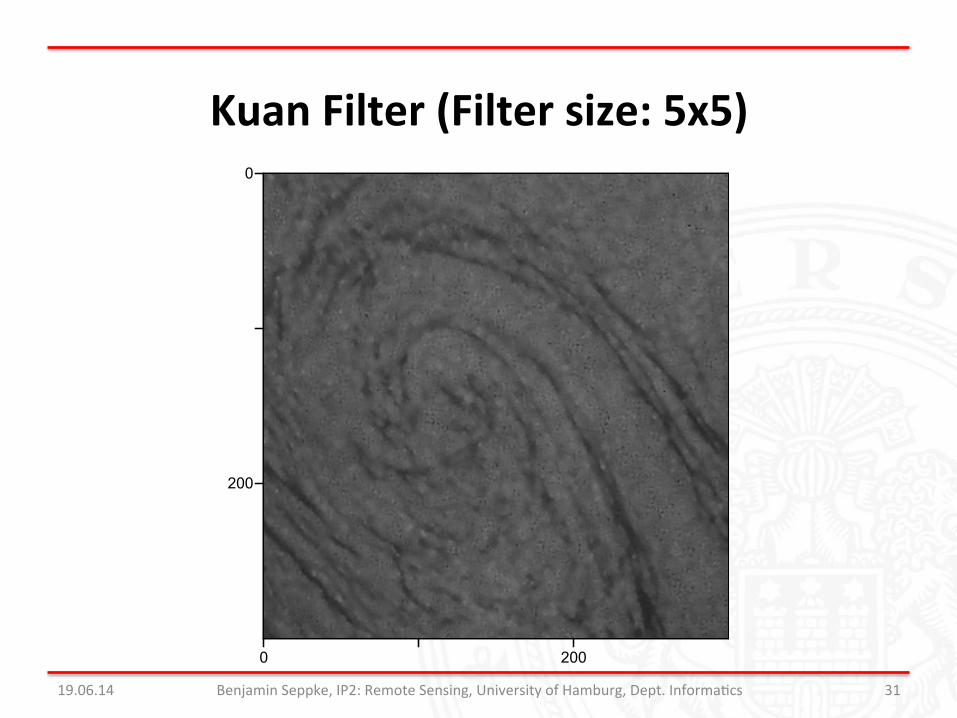
Kuan Filter (Filter size: 5x5)
19.06.14 Benjamin Seppke, IP2: Remote Sensing, University of Hamburg, Dept. InformaJcs 31
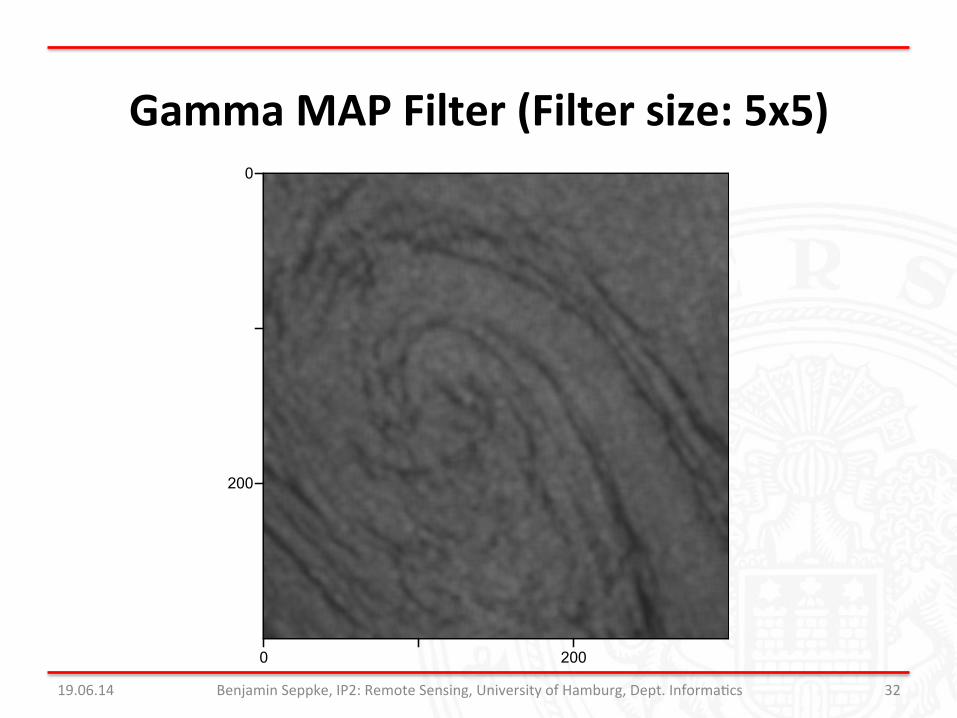
Gamma MAP Filter (Filter size: 5x5)
19.06.14 Benjamin Seppke, IP2: Remote Sensing, University of Hamburg, Dept. InformaJcs 32

Frost Filter (k=1, Filter size: 5x5)
19.06.14 Benjamin Seppke, IP2: Remote Sensing, University of Hamburg, Dept. InformaJcs 33
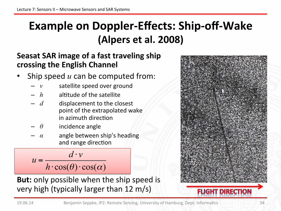
Example on Doppler-‐Effects: Ship-‐off-‐Wake (Alpers et al. 2008)
Seasat SAR image of a fast traveling ship crossing the English Channel • Ship speed u can be computed from:
– v satellite speed over ground – h alJtude of the satellite – d displacement to the closest
point of the extrapolated wake in azimuth direcJon
– θ incidence angle – α angle between ship’s heading
and range direcJon
But: only possible when the ship speed is very high (typically larger than 12 m/s) 19.06.14 Benjamin Seppke, IP2: Remote Sensing, University of Hamburg, Dept. InformaJcs 34
Lecture 7: Sensors II – Microwave Sensors and SAR Systems
u = d ⋅ vh ⋅cos(θ ) ⋅cos(α)
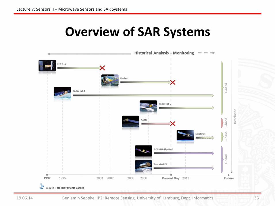
Overview of SAR Systems
19.06.14 Benjamin Seppke, IP2: Remote Sensing, University of Hamburg, Dept. InformaJcs 35
Lecture 7: Sensors II – Microwave Sensors and SAR Systems
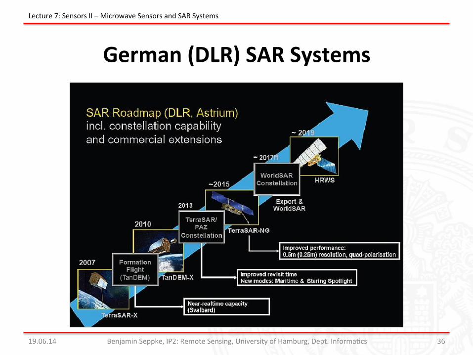
German (DLR) SAR Systems
19.06.14 Benjamin Seppke, IP2: Remote Sensing, University of Hamburg, Dept. InformaJcs 36
Lecture 7: Sensors II – Microwave Sensors and SAR Systems
Issues for High-‐Resolu7on SAR Imagery
• New SAR Systems achieve resoluJons of < ½ m! • Formerly unknown details become visible • Direct backscaKering “paints” the scene • Huge impact on observaJon of man-‐made scenes, like:
– CiJes / Buildings – Ships – Infrastructure
• Weather independent observaJon of these structures is of high military interest à German Bundeswehr: SAR-‐Lupe (5 equal hi-‐res SAR)
19.06.14 Benjamin Seppke, IP2: Remote Sensing, University of Hamburg, Dept. InformaJcs 37
Lecture 7: Sensors II – Microwave Sensors and SAR Systems
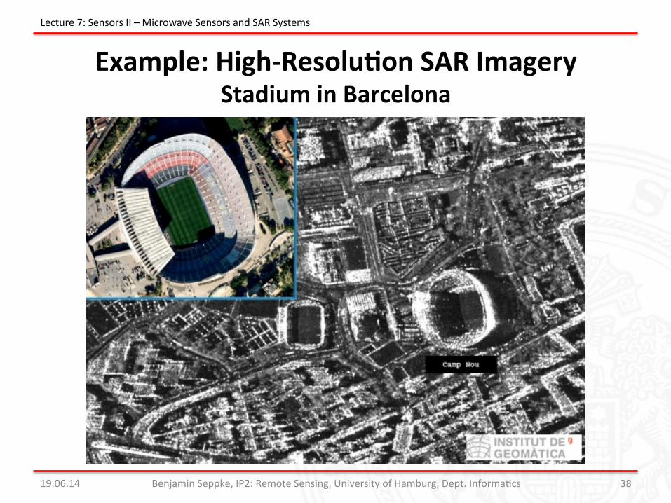
Example: High-‐Resolu7on SAR Imagery Stadium in Barcelona
19.06.14 Benjamin Seppke, IP2: Remote Sensing, University of Hamburg, Dept. InformaJcs 38
Lecture 7: Sensors II – Microwave Sensors and SAR Systems
Interferometric SAR (InSAR)
• Uses the phase instead of using the magnitude image • Distance between two acquisiJons: baseline • Requirements of the baseline
– needs to be small for a high correlaJon of the “persistent” scaKerers! – needs to be large enough to actually determine phase shizs!
• Former: Use of two or more different satellites! • Now: Special configuraJons allow the derivaJon of InSAR
images with comparable sensors or with a single pla�orm. • Basic measurement:
(Changes in the) Terrain of the surface
19.06.14 Benjamin Seppke, IP2: Remote Sensing, University of Hamburg, Dept. InformaJcs 39
Lecture 7: Sensors II – Microwave Sensors and SAR Systems
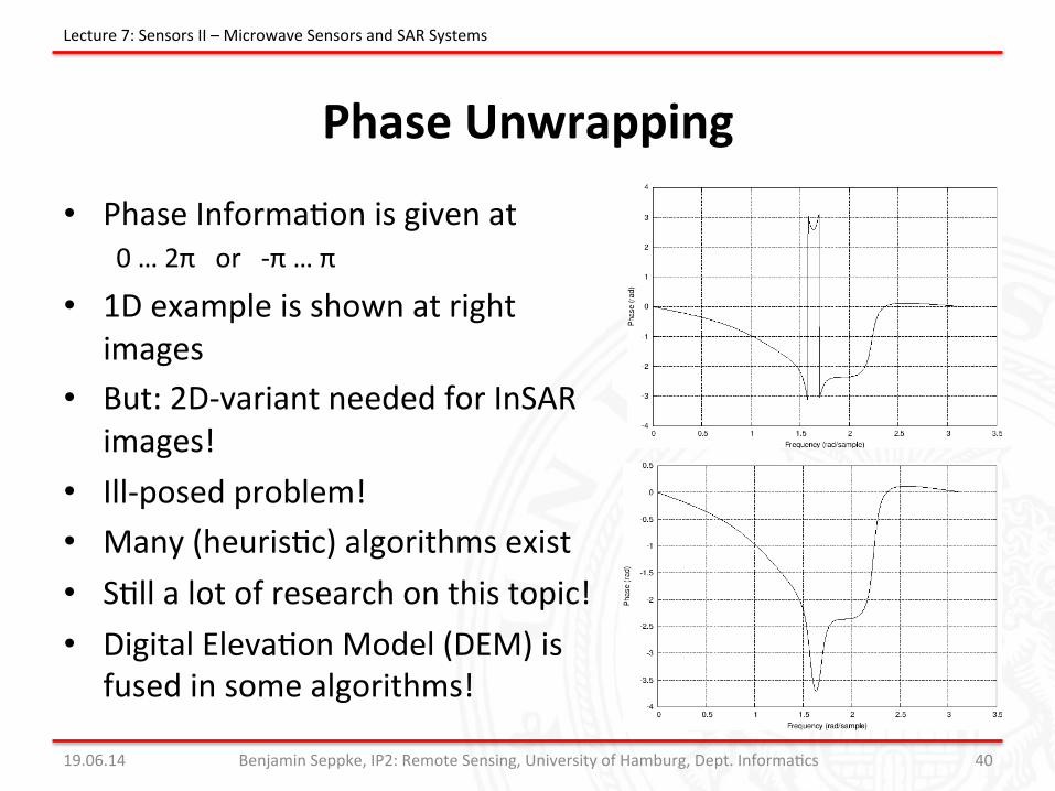
Phase Unwrapping
• Phase InformaJon is given at 0 … 2π or -‐π … π
• 1D example is shown at right images
• But: 2D-‐variant needed for InSAR images!
• Ill-‐posed problem! • Many (heurisJc) algorithms exist • SJll a lot of research on this topic! • Digital ElevaJon Model (DEM) is
fused in some algorithms! 19.06.14 Benjamin Seppke, IP2: Remote Sensing, University of Hamburg, Dept. InformaJcs 40
Lecture 7: Sensors II – Microwave Sensors and SAR Systems
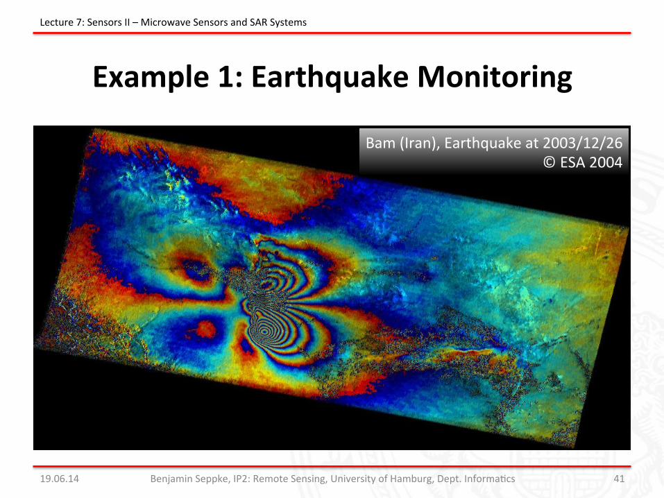
Example 1: Earthquake Monitoring
19.06.14 Benjamin Seppke, IP2: Remote Sensing, University of Hamburg, Dept. InformaJcs 41
Lecture 7: Sensors II – Microwave Sensors and SAR Systems
Bam (Iran), Earthquake at 2003/12/26 © ESA 2004
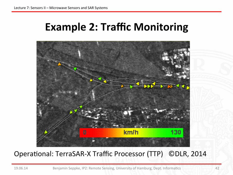
Example 2: Traffic Monitoring
OperaJonal: TerraSAR-‐X Traffic Processor (TTP) ©DLR, 2014
19.06.14 Benjamin Seppke, IP2: Remote Sensing, University of Hamburg, Dept. InformaJcs 42
Lecture 7: Sensors II – Microwave Sensors and SAR Systems
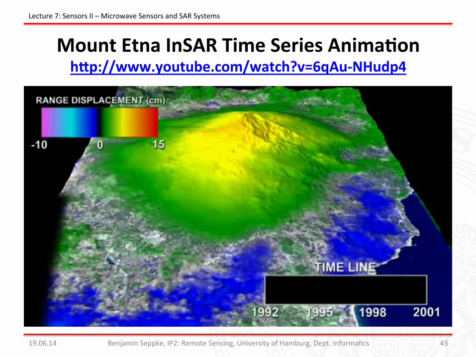
Mount Etna InSAR Time Series Anima7on hKp://www.youtube.com/watch?v=6qAu-‐NHudp4
19.06.14 Benjamin Seppke, IP2: Remote Sensing, University of Hamburg, Dept. InformaJcs 43
Lecture 7: Sensors II – Microwave Sensors and SAR Systems