INVESTIGATION OF ELLIPTICAL COOLING CHANNELS … · Investigation of elliptical cooling channels...
97
U.S.N.A --- Trident Scholar project report; no. 338 (2005) INVESTIGATION OF ELLIPTICAL COOLING CHANNELS FOR A NAVAL ELECTROMAGNETIC RAILGUN by Midshipman 1/c Elizabeth R. Kealey, Class of 2005 United States Naval Academy Annapolis, MD ___________________________________ (signature) Certification of Advisers Approval Assistant Professor Peter J. Joyce Mechanical Engineering Department ___________________________________ (signature) ______________________ (date) Assistant Professor Andrew N. Smith Mechanical Engineer Department ___________________________________ (signature) ______________________ (date) Acceptance for the Trident Scholar Committee Professor Joyce E. Shade Deputy Director of Research & Scholarship ___________________________________ (signature) ______________________ (date) USNA-1531-2
Transcript of INVESTIGATION OF ELLIPTICAL COOLING CHANNELS … · Investigation of elliptical cooling channels...

U.S.N.A --- Trident Scholar project report; no. 338 (2005)
INVESTIGATION OF ELLIPTICAL COOLING CHANNELS FOR A NAVAL ELECTROMAGNETIC RAILGUN
by
Midshipman 1/c Elizabeth R. Kealey, Class of 2005 United States Naval Academy
Annapolis, MD
___________________________________ (signature)
Certification of Advisers Approval
Assistant Professor Peter J. Joyce
Mechanical Engineering Department
___________________________________ (signature)
______________________ (date)
Assistant Professor Andrew N. Smith Mechanical Engineer Department
___________________________________
(signature) ______________________
(date)
Acceptance for the Trident Scholar Committee
Professor Joyce E. Shade
Deputy Director of Research & Scholarship
___________________________________ (signature)
______________________ (date)
USNA-1531-2

REPORT DOCUMENTATION PAGE
Form Approved OMB No. 074-0188
Public reporting burden for this collection of information is estimated to average 1 hour per response, including g the time for reviewing instructions, searching existing data sources, gathering and maintaining the data needed, and completing and reviewing the collection of information. Send comments regarding this burden estimate or any other aspect of the collection of information, including suggestions for reducing this burden to Washington Headquarters Services, Directorate for Information Operations and Reports, 1215 Jefferson Davis Highway, Suite 1204, Arlington, VA 22202-4302, and to the Office of Management and Budget, Paperwork Reduction Project (0704-0188), Washington, DC 20503. 1. AGENCY USE ONLY (Leave blank)
2. REPORT DATE 9 May 2005
3. REPORT TYPE AND DATE COVERED
4. TITLE AND SUBTITLE Investigation of elliptical cooling channels for a naval electromagnetic railgun 6. AUTHOR(S) Kealey, Elizabeth R. (Elizabeth Rose), 1982-
5. FUNDING NUMBERS
7. PERFORMING ORGANIZATION NAME(S) AND ADDRESS(ES)
8. PERFORMING ORGANIZATION REPORT NUMBER
9. SPONSORING/MONITORING AGENCY NAME(S) AND ADDRESS(ES)
10. SPONSORING/MONITORING AGENCY REPORT NUMBER
US Naval Academy Annapolis, MD 21402
Trident Scholar project report no. 338 (2005)
11. SUPPLEMENTARY NOTES
12a. DISTRIBUTION/AVAILABILITY STATEMENT This document has been approved for public release; its distribution is UNLIMITED.
12b. DISTRIBUTION CODE
13. ABSTRACT: The future Naval Electromagnetic Railgun will use a mega-ampere electrical current to generate an electromagnetic force which accelerates a projectile to hypersonic velocities. The applied current can raise the bulk temperature of the rails by over 100 degrees Celsius, necessitating an active cooling system for the rails to sustain high rates of fire without incurring permanent damage to the gun. The electromagnetic force on the projectile and the rails creates a complicated stress state that varies as the projectile passes along the rail, first uniaxial then biaxial compression acts on the rails. In this study, a system of cooling channels for fluid flow down the length of the rails was considered, and channels with elliptical cross sections were examined. Elliptical shapes were considered due to the high surface area available for convection, relatively low impact on the stress distribution, and low stress concentration effect. By treating an elliptical channel as a variable area fin and varying the size and aspect ratio of the ellipse and the distance between channels, the heat transfer capability of a channel array was maximized based on given flow conditions and applied heat flux. The optimal channel design was further constrained by the applied compressive stresses. It was found that ellipses of different aspect ratios are optimal for the uniaxial and biaxial stress states, and the optimal channel design was limited by the competing effects of these two structural constraints. In order to test the thermal aspect of the design, a representative set of channels were machined into one third scale copper rails using wire electrical discharge machining. Tests were performed using both a steady state heat flux to determine the overall heat transfer coefficient and transient conditions to determine the system thermal relaxation time. In order to verify the structural aspect of the design, a finite element analysis was done on the rail cross section to compare the computational stress concentration factors with the theoretical correlations used in the literature. The results of both the thermal experiments and finite element analysis were found to be in reasonable agreement with the predicted results. .
15. NUMBER OF PAGES 95
14. SUBJECT TERMS: Electromagnetic Railgun; Elliptical Cooling Channels; Thermal anagement; Cooling Channel Optimization 16. PRICE CODE
17. SECURITY CLASSIFICATION OF REPORT
18. SECURITY CLASSIFICATION OF THIS PAGE
19. SECURITY CLASSIFICATION OF ABSTRACT
20. LIMITATION OF ABSTRACT
NSN 7540-01-280-5500 Standard Form 298 (Rev.2-89) Prescribed by ANSI Std. Z39-18
298-102

1
ABSTRACT
The future Naval Electromagnetic Railgun will use a mega-ampere electrical current to generate an electromagnetic force which accelerates a projectile to hypersonic velocities. The applied current can raise the bulk temperature of the rails by over 100 degrees Celsius, necessitating an active cooling system for the rails to sustain high rates of fire without incurring permanent damage to the gun. The electromagnetic force on the projectile and the rails creates a complicated stress state that varies as the projectile passes along the rail, first uniaxial then biaxial compression acts on the rails.
In this study, a system of cooling channels for fluid flow down the length of the rails was considered, and channels with elliptical cross sections were examined. Elliptical shapes were considered due to the high surface area available for convection, relatively low impact on the stress distribution, and low stress concentration effect. By treating an elliptical channel as a variable area fin and varying the size and aspect ratio of the ellipse and the distance between channels, the heat transfer capability of a channel array was maximized based on given flow conditions and applied heat flux. The optimal channel design was further constrained by the applied compressive stresses. It was found that ellipses of different aspect ratios are optimal for the uniaxial and biaxial stress states, and the optimal channel design was limited by the competing effects of these two structural constraints.
In order to test the thermal aspect of the design, a representative set of channels were machined into one third scale copper rails using wire electrical discharge machining. Tests were performed using both a steady state heat flux to determine the overall heat transfer coefficient and transient conditions to determine the system thermal relaxation time. In order to verify the structural aspect of the design, a finite element analysis was done on the rail cross section to compare the computational stress concentration factors with the theoretical correlations used in the literature. The results of both the thermal experiments and finite element analysis were found to be in reasonable agreement with the predicted results.
Keywords: Electromagnetic Railgun; Elliptical Cooling Channels; Thermal Management; Cooling Channel Optimization

2
ACKNOWLEDGEMENTS
This project would have never been possible without the gracious support from many people. The Technical Support Division of Rickover Hall provided assistance in the entire process, from manufacturing and purchasing parts to implementation of the experiment. Several members of the support staff supported this project in particular: Bob Woody, Bob Banks, Charlie Popp, Tom Price, and Jerry Myers. I would like to extend a special thanks to Charlie Popp for his patience, expertise and willingness to help me at every step of my experiment. The progress of this project is also a major reflection of the effort of my two advisors, Assistant Professors Peter Joyce and Andrew Smith. Their instruction and mentoring was an invaluable resource for both me and this project.

3
TABLE OF CONTENTS
Abstract 1 Acknowledgements 2 Table of Contents 3 List of Figures 5 Nomenclature 7 List of Equations 9 1.0 Introduction 11 1.1 The Need for a Long Range Naval Gun 1.2 The Electromagnetic Railgun 1.3 Thermal Management of a Railgun Launcher 1.4 Forces on the Rails 2.0 Design of an Optimal Channel Cross Section 17 2.1 Initial Assumptions 2.2 Heat Transfer in an Elliptical Fin 2.3 Structural Constraints 2.4 Optimization Routine 3.0 Design of an Optimal Channel for a Full Scale Railgun 30 3.1 Initial Design Choices 3.2 Results 3.3 Design Conclusion 3.4 Implications of Cooling Channel Design 4.0 Experimental Configuration 38 4.1 Scaled Parameters 4.2 Optimized Experimental Design 4.3 Experimental Channel Shapes 5.0 Finite Element Analysis of Design 41 5.1 Uniaxial Stress Concentration Factor from I-DEAS
5.2 Biaxial Stress Concentration Factor from I-DEAS 5.3 Finite Element Analysis Conclusions
6.0 Experimental Verification of Heat Transfer Ability under 48
Steady State Conditions 6.1 Experimental Set-Up 6.2 Data Acquisition 6.3 Data Analysis and Results 7.0 Transient Considerations 57 7.1 Finite Difference Model of the Transient Thermal Response

4
7.2 Experimental Verification of Transient Model 8.0 Conclusions 64 Bibliography 66 Appendix 1: Optimization Code (Matlab®) 67 Appendix 2: Optimization Results 73 Appendix 3: Average Surface Temperature Calculations (Matlab®) 75 Appendix 4: Finite Element Analysis: Uniaxial Stress 76 Appendix 5: Finite Element Analysis: Infinite Biaxial Stress 81 Appendix 6: Finite Element Analysis: Finite Biaxial Stress 82 Appendix 7: G-10 Material Properties 83 Appendix 8: Thermocouple Calibration (Matlab®) 84 Appendix 9: Steady State Test Data (Matlab®) 85 Appendix 10: Steady State Data Calculations 87 Appendix 11: Transient Model (Matlab®) 89 Appendix 12: Material Properties Search: Possible Rail Materials 95

5
LIST OF FIGURES
Figure 1: Schematic showing the basic principles of an EM Railgun 10 Figure 2: Current discharge from a pulse forming network vs. time 11 Figure 3: Energy distribution from a single railgun shot 12 Figure 4: Rail cross section under uniaxial compression 13 Figure 5: a) Magnetic field on half of a rail cross section 14 Figure 5: b) Linear current density around the perimeter of a rail 14 Figure 6: Uniform biaxial stresses on a rail cross section 14 Figure 7: Rail Cross section with one insulated thermal boundaries 16 Figure 8: Three unit cells in a rail cross section with possible channel shapes 17 Figure 9: An array of fins used as a heat sink. 17 Figure 10: Half section of a fin model 18 Figure 11: Boundary conditions for the fin model 19 Figure 12: Temperature profile as a function of position along the x axis 20 Figure 13: Uniaxial compression on a unit cell 21 Figure 14: Uniaxial stress concentration factor vs. λ 23 Figure 15: a) Finite width plate with unconstrained edges 24 Figure 15: b) unit cell with supported edges 24 Figure 16: Infinite plate subject to biaxial loading 25 Figure 17: Biaxial stress concentration factor vs. biaxial stress ratio 25 Figure 18: Biaxial compression on a unit cell 27 Figure 19: Rail with channels 20 mm from edge 29 Figure 20: Unit cell resistance vs. number of cells 31 Figure 21: Total Resistance vs. number of channels 32 Figure 22: Heat transfer coefficient vs. number of cells 33 Figure 23: a) Aspect ratio vs. number of cells 34 Figure 23: b) Channel width ratio vs. number of cells 34 Figure 24: Optimal Channel Arrays for 12, 8 and 4 unit cells 35 Figure 25: Optimized Design for the experimental rail 37 Figure 26: Fin resistance vs. ellipse half length (b) 37 Figure 27: Quarter unit cell with forces and constraints shown 39 Figure 28: I-DEAS: Quarter of a circular hole in uniaxial compression 40 Figure 29: I-DEAS: Approximation of an infinite plane 41 Figure 30: Stress Concentration Factor vs. Stress Ratio for Aspect Ratio of 1.0. 42 Figure 31: Stress Concentration Factor vs. Stress Ratio for Aspect Ratio of 2.0. 42 Figure 32: Stress Concentration Factor vs. Stress Ratio for Aspect Ratio of 2.0. 43 Figure 33: Finite width unit cell in biaxial compression 44 Figure 34: Stress Concentration factor vs. stress ratio (aspect ratio 1.844) 44 Figure 35: Three experimental channels 46 Figure 36: Kapton heater applied to rail surface 47 Figure 37: G-10 Containment 47 Figure 38: a) Manifold device 48 Figure 38: b) Manifold device connected to the rail. 48 Figure 39: Diagram showing thermocouple location 49

6
Figure 40: Rail #1: Temperature Difference vs. Position 51 Figure 41: Rail #2: Temperature Difference vs. Position 51 Figure 42: Rail #3: Temperature Difference vs. Position 52 Figure 43: Rfin vs. flow rate for all three rails 53 Figure 44: Unit cell half section, with nodes and elements identified 55 Figure 45: a) Single node with nodal temperatures and heat terms 55 Figure 45: b) Single node with geometric parameters defined 55 Figure 46: a) Temperature profile in a 1.0 second interval 57 Figure 46: b) Temperature profile in a 1.0 second interval 58 Figure 47: Temperature profile along bar 59 Figure 48: Temperature at thermocouple 10 vs. time 60 Figure 49: Experimental and Theoretical Q/Qo ratios 61 Figure 50: Rail surface temperature vs. steady state cooling time 62
LIST OF TABLES Table 1: Input variables for optimization function 28 Table 2: Notional Naval Railgun Parameters 29 Table 3: Stresses for a full size and scaled rail 36 Table 4: Experimental Rail Parameters 38 Table 5: Test matrix 49 Table 6: Q/Qo ratios at given times 58

7
NOMENCLATURE
a Elliptical channel half height (m) Abore Bore cross sectional area (m2) Ac Fin cross sectional area (m2) Aellipse Area of an ellipse (m2) As Surface area (m2) b Elliptical channel half width (m) Cp Fluid specific heat (J/kgK) d Distance between front edge of the rail and the “top” of the ellipse (m) Dh Hydraulic diameter (m) f Friction factor F Force (N) FS Factor of Safety h Heat transfer coefficient (W/m2-K) I Electrical current (A) K Stress concentration factor Kuniaxial Uniaxial stress concentration factor Kbiaxial Biaxial stress concentration factors kf, ks Fluid and solid thermal conductivities (W/m-K) L′ Inductance per unit length (µH/m) N Number of unit cells in a rail Nu Nusselt number
p′∆ Pressure drop per unit length (Pa/m) Pr Prandtl number Pellipse Perimeter of an ellipse (m) qfin Fin heat transfer rate (W)
finq′ Fin heat transfer rate per unit length (W/m) qcond Conduction heat transfer rate (W)
condq′ Conduction heat transfer rate per unit length (W/m) Re Reynolds number Rfin Fin resistance (K/W) TS Fin surface temperature (K) T∞ Bulk fluid temperature (K) t Minimum fin half thickness (m) Um Fluid mean velocity (m/s) V& Volumetric flow rate (m3/s)
totalW ′& Pump power per unit length (W/m) x, y Cartesian coordinates for a unit cell (m) y* Local fin height, (a + t - y) (m)
Greek Symbols
β Ellipse aspect ratio (b/a) ρ Fluid density (kg/m3)

8
σ Stress (MPa) σuniaxial Uniaxial Stress (MPa) σ1, σ2 Biaxial Stresses (MPa) θ Difference between solid and bulk fluid temperatures, TS – T∞ (K) µ Dynamic viscosity (kg/m3) λ Channel width ratio (a/(a+t)) (m)

9
LIST OF EQUATIONS
Equation 1: Force as a function of magnetic field and current density 13 Equation 2: Stress concentration factor definition 15 Equation 3: Definition of Rfin 17 Equation 4: General energy equation for a variable area fin 18 Equation 5: Energy equation for a fin with elliptical boundaries 18 Equation 6: Equation for local fin height (y*) 18 Equation 7: Energy equation boundary conditions 18 Equation 8: Fin heat transfer rate 19 Equation 9: Fin heat transfer rate per unit length 19 Equation 10: Channel pump power 20 Equation 11: Area of an ellipse 20 Equation 12: Perimeter of an ellipse 20 Equation 13: Hydraulic diameter 21 Equation 14: Nusselt number definition 21 Equation 15: Nusselt number correlation 21 Equation 16: Reynolds number defintion 21 Equation 17: Volumetric flow rate 21 Equation 18: Pump power and pressure loss relationship 21 Equation 19: Pressure loss 21 Equation 20: Friction factor 21 Equation 21: Uniaxial maximum stress 22 Equation 22: Uniaxial nominal stress 22 Equation 23: Channel width ratio 22 Equation 24: Aspect ratio, β defined 22 Equation 25: Uniaxial stress concentration factor 22 Equation 26: Uniaxial stress constraint 24 Equation 27: Allowable stress 24 Equation 28: Condition for maximum stress at point A 26 Equation 29: Condition for maximum stress at point B 26 Equation 30: Biaxial maximum stress 26 Equation 31: Biaxial stress concentration factor 26 Equations 32-32: Biaxial nominal stresses 26 Equation 34: Biaxial maximum stress based on nominal stresses 26 Equation 35: Biaxial maximum stress constraint 27 Equation 36: Allowable stress 27 Equation 37: I-DEAS Uniaxial stress concentration factor 40 Equation 38: Average water inlet temperature 49 Equation 39: Average water outlet temperature 50 Equation 40: Water temperature as a function of z 50 Equation 41: Thermal entry length 50 Equation 42: Overall heat transfer coefficient 52 Equation 43: Fin thermal resistance 52 Equation 44: Average fin thermal resistance 52 Equation 45: General heat equation for a transient system 55

10
Equation 46: Fourier number 55 Equation 47: General heat equation with coefficients a, b, c, and d 55 Equation 48: Tridiagonal matrix 55 Equation 49: Average final bar temperature 58 Equation 50: Heat ratio, Q/Qo 58
11
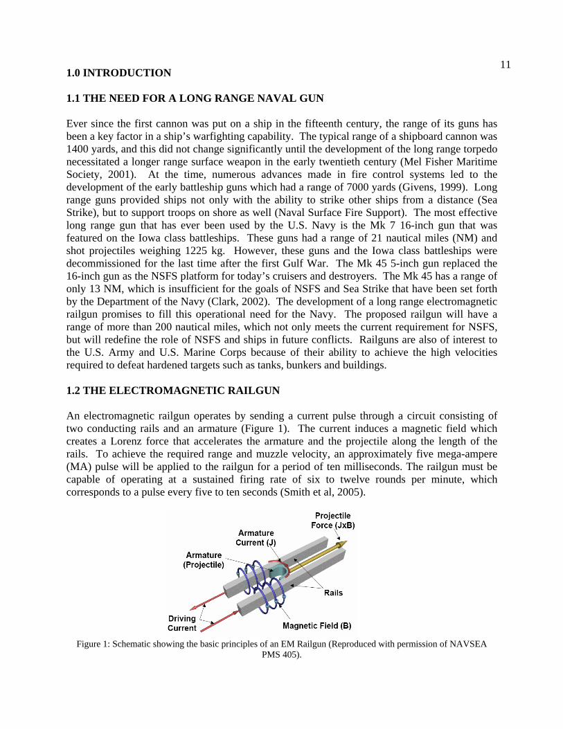
1.0 INTRODUCTION 1.1 THE NEED FOR A LONG RANGE NAVAL GUN Ever since the first cannon was put on a ship in the fifteenth century, the range of its guns has been a key factor in a ship’s warfighting capability. The typical range of a shipboard cannon was 1400 yards, and this did not change significantly until the development of the long range torpedo necessitated a longer range surface weapon in the early twentieth century (Mel Fisher Maritime Society, 2001). At the time, numerous advances made in fire control systems led to the development of the early battleship guns which had a range of 7000 yards (Givens, 1999). Long range guns provided ships not only with the ability to strike other ships from a distance (Sea Strike), but to support troops on shore as well (Naval Surface Fire Support). The most effective long range gun that has ever been used by the U.S. Navy is the Mk 7 16-inch gun that was featured on the Iowa class battleships. These guns had a range of 21 nautical miles (NM) and shot projectiles weighing 1225 kg. However, these guns and the Iowa class battleships were decommissioned for the last time after the first Gulf War. The Mk 45 5-inch gun replaced the 16-inch gun as the NSFS platform for today’s cruisers and destroyers. The Mk 45 has a range of only 13 NM, which is insufficient for the goals of NSFS and Sea Strike that have been set forth by the Department of the Navy (Clark, 2002). The development of a long range electromagnetic railgun promises to fill this operational need for the Navy. The proposed railgun will have a range of more than 200 nautical miles, which not only meets the current requirement for NSFS, but will redefine the role of NSFS and ships in future conflicts. Railguns are also of interest to the U.S. Army and U.S. Marine Corps because of their ability to achieve the high velocities required to defeat hardened targets such as tanks, bunkers and buildings. 1.2 THE ELECTROMAGNETIC RAILGUN An electromagnetic railgun operates by sending a current pulse through a circuit consisting of two conducting rails and an armature (Figure 1). The current induces a magnetic field which creates a Lorenz force that accelerates the armature and the projectile along the length of the rails. To achieve the required range and muzzle velocity, an approximately five mega-ampere (MA) pulse will be applied to the railgun for a period of ten milliseconds. The railgun must be capable of operating at a sustained firing rate of six to twelve rounds per minute, which corresponds to a pulse every five to ten seconds (Smith et al, 2005).
Figure 1: Schematic showing the basic principles of an EM Railgun (Reproduced with permission of NAVSEA
PMS 405).
12
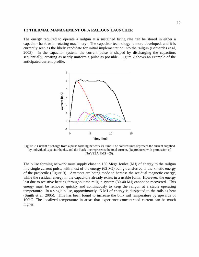
1.3 THERMAL MANAGEMENT OF A RAILGUN LAUNCHER The energy required to operate a railgun at a sustained firing rate can be stored in either a capacitor bank or in rotating machinery. The capacitor technology is more developed, and it is currently seen as the likely candidate for initial implementation into the railgun (Bernardes et al, 2003). In the capacitor system, the current pulse is shaped by discharging the capacitors sequentially, creating as nearly uniform a pulse as possible. Figure 2 shows an example of the anticipated current profile.
Figure 2: Current discharge from a pulse forming network vs. time. The colored lines represent the current supplied by individual capacitor banks, and the black line represents the total current. (Reproduced with permission of
NAVSEA PMS 405).
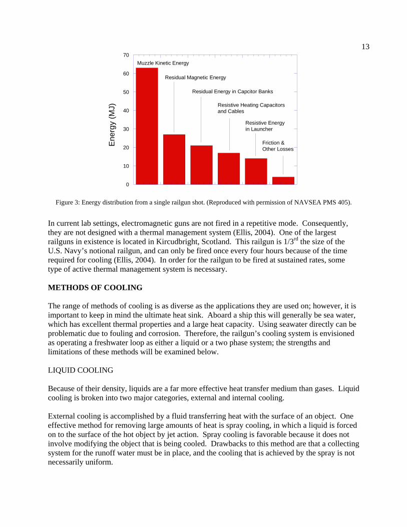
The pulse forming network must supply close to 150 Mega Joules (MJ) of energy to the railgun in a single current pulse, with most of the energy (63 MJ) being transferred to the kinetic energy of the projectile (Figure 3). Attempts are being made to harness the residual magnetic energy, while the residual energy in the capacitors already exists in a usable form. However, the energy lost due to resistive heating throughout the railgun system (30-40 MJ) cannot be recovered. This energy must be removed quickly and continuously to keep the railgun at a stable operating temperature. In a single pulse, approximately 15 MJ of energy is dissipated to the rails as heat (Smith et al, 2005). This has been found to increase the bulk rail temperature by upwards of 100ºC. The localized temperature in areas that experience concentrated current can be much higher.
-1
0
1
2
3
4
5
6
0 5 10 15
Time [ms]
Curr
ent [
MA]
13
0
10
20
30
40
50
60
70
Ene
rgy
(MJ)
Muzzle Kinetic Energy
Residual Magnetic Energy
Residual Energy in Capcitor Banks
Resistive Energy in Launcher
Friction & Other Losses
Resistive Heating Capacitors and Cables
Figure 3: Energy distribution from a single railgun shot. (Reproduced with permission of NAVSEA PMS 405).
In current lab settings, electromagnetic guns are not fired in a repetitive mode. Consequently, they are not designed with a thermal management system (Ellis, 2004). One of the largest railguns in existence is located in Kircudbright, Scotland. This railgun is 1/3rd the size of the U.S. Navy’s notional railgun, and can only be fired once every four hours because of the time required for cooling (Ellis, 2004). In order for the railgun to be fired at sustained rates, some type of active thermal management system is necessary. METHODS OF COOLING The range of methods of cooling is as diverse as the applications they are used on; however, it is important to keep in mind the ultimate heat sink. Aboard a ship this will generally be sea water, which has excellent thermal properties and a large heat capacity. Using seawater directly can be problematic due to fouling and corrosion. Therefore, the railgun’s cooling system is envisioned as operating a freshwater loop as either a liquid or a two phase system; the strengths and limitations of these methods will be examined below. LIQUID COOLING Because of their density, liquids are a far more effective heat transfer medium than gases. Liquid cooling is broken into two major categories, external and internal cooling. External cooling is accomplished by a fluid transferring heat with the surface of an object. One effective method for removing large amounts of heat is spray cooling, in which a liquid is forced on to the surface of the hot object by jet action. Spray cooling is favorable because it does not involve modifying the object that is being cooled. Drawbacks to this method are that a collecting system for the runoff water must be in place, and the cooling that is achieved by the spray is not necessarily uniform.

14
Internal cooling involves passing a liquid through some type of channel imbedded in the material being cooled. Advantages to this system are that the inner part of an object can be directly cooled, and the cooling is uniform along the length of the channel as the liquid is contained in a closed loop process. The disadvantage is that the cooling channels reduce the structural integrity of the object being cooled. TWO PHASE COOLING Excellent heat transfer is possible from a system where a liquid is allowed to vaporize. The heat transfer coefficient in this process is at least two orders of magnitude larger than the heat transfer coefficient for a liquid that does not change phase. Difficulties in implementing a system like this include the high temperatures involved in vaporization and the pressure changes that are associated with it. These systems tend to be more complex and difficult to operate than liquid cooling systems. COOLING THE RAILGUN’S RAILS Liquid internal cooling has been chosen by the Navy as the most promising method for cooling the rails. Air cooling does not have the ability to transfer heat quickly enough for railgun applications, spray cooling was considered too difficult to accomplish within an electrically charged gun bore, and the pressure changes associated with two phase cooling introduce too many complications to the design process. 1.4 FORCES ON THE RAILS As the current heats the rails, it also causes an electromagnetic force that acts on the rails (Figure 4). The acceleration force on the projectile can be calculated from the current (I) and the inductance gradient ( L′ ) of the rails as shown below (Bernardes et al, 2003). The same magnetic pressure that is accelerating the projectile also acts to push the rails apart. Therefore, the acceleration force on the projectile can be used to find the compressive force on the rails.
2
21 ILF ′= (1)
Figure 4: Rail cross section under uniaxial compression.
15
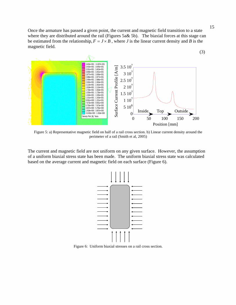
Once the armature has passed a given point, the current and magnetic field transition to a state where they are distributed around the rail (Figures 5a& 5b). The biaxial forces at this stage can be estimated from the relationship, F J B= × , where J is the linear current density and B is the magnetic field. (3)
05 1061 107
1.5 1072 107
2.5 1073 107
3.5 107
0 50 100 150 200Surfa
ce C
urre
nt P
rofil
e [A
/m]
Position [mm]
Inside OutsideTop
Figure 5: a) Representative magnetic field on half of a rail cross section. b) Linear current density around the
perimeter of a rail (Smith et al, 2005)
The current and magnetic field are not uniform on any given surface. However, the assumption of a uniform biaxial stress state has been made. The uniform biaxial stress state was calculated based on the average current and magnetic field on each surface (Figure 6).
Figure 6: Uniform biaxial stresses on a rail cross section.
Density Plot: |B|, Tesla
3.645e+001 : >3.837e+0013.453e+001 : 3.645e+0013.261e+001 : 3.453e+0013.069e+001 : 3.261e+0012.877e+001 : 3.069e+0012.686e+001 : 2.877e+0012.494e+001 : 2.686e+0012.302e+001 : 2.494e+0012.110e+001 : 2.302e+0011.918e+001 : 2.110e+0011.726e+001 : 1.918e+0011.535e+001 : 1.726e+0011.343e+001 : 1.535e+0011.151e+001 : 1.343e+0019.591e+000 : 1.151e+0017.673e+000 : 9.591e+0005.755e+000 : 7.673e+0003.837e+000 : 5.755e+0001.918e+000 : 3.837e+000<0.000e+000 : 1.918e+000
16
STRESS CONCENTRATION FACTORS An abrupt change in the geometry of an object can cause an uneven stress distribution, where the stress near the change in form is much higher than the stress in the rest of the object. This effect is seen near holes, fillets, notches and even scratches in a material (Spotts and Shoup, 1998). A stress concentration factor (K) is used to describe the ratio of local maximum stress to applied stress (Eq. 2).
maximum
applied
K σσ
= (2)
Published theoretical equations, experimental measurements and finite element analysis can all be used to determine the stress concentration factor for a particular geometry. Due to the ease of manufacturing, cooling channels typically have a circular cross section, which has a relatively low stress concentration factor (K = 3) (Peterson, 1953).
17
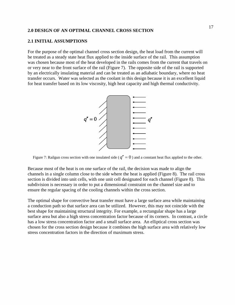
2.0 DESIGN OF AN OPTIMAL CHANNEL CROSS SECTION 2.1 INITIAL ASSUMPTIONS For the purpose of the optimal channel cross section design, the heat load from the current will be treated as a steady state heat flux applied to the inside surface of the rail. This assumption was chosen because most of the heat developed in the rails comes from the current that travels on or very near to the front surface of the rail (Figure 7). The opposite side of the rail is supported by an electrically insulating material and can be treated as an adiabatic boundary, where no heat transfer occurs. Water was selected as the coolant in this design because it is an excellent liquid for heat transfer based on its low viscosity, high heat capacity and high thermal conductivity.
Figure 7: Railgun cross section with one insulated side ( 0=′′q ) and a constant heat flux applied to the other.
Because most of the heat is on one surface of the rail, the decision was made to align the channels in a single column close to the side where the heat is applied (Figure 8). The rail cross section is divided into unit cells, with one unit cell designated for each channel (Figure 8). This subdivision is necessary in order to put a dimensional constraint on the channel size and to ensure the regular spacing of the cooling channels within the cross section. The optimal shape for convective heat transfer must have a large surface area while maintaining a conduction path so that surface area can be utilized. However, this may not coincide with the best shape for maintaining structural integrity. For example, a rectangular shape has a large surface area but also a high stress concentration factor because of its corners. In contrast, a circle has a low stress concentration factor and a small surface area. An elliptical cross section was chosen for the cross section design because it combines the high surface area with relatively low stress concentration factors in the direction of maximum stress.
q ′′0=′′q q ′′0=′′q

18
Figure 8: Three unit cells in a rail cross section with possible cooling channel shapes.
2.2 HEAT TRANSFER IN AN ELLIPTICAL FIN A solid that experiences conduction within its boundaries and convection between its surface and the surroundings is called an extended surface. When the extended surface is specifically designed to increase the rate of heat transfer between the surface and the surrounding fluid it is called a fin (Incropera and DeWitt, 2002), an example of an array of fins is shown in Figure 9. Fins can take on many forms and they are widely used in applications such as engine heads, air conditioners and computer chips.
Figure 9: An array of fins used as a heat sink. The thermal performance of a fin is characterized by the thermal resistance of the fin, Rfin which is computed as follows:
.finfin
Rqθ
= (3)
where θ is the difference between the temperature of at the base of the fin, Tx=0 and the bulk fluid temperature, T∞; and qfin is the rate of heat transfer in the fin.
Insufficient surface area for convection
Insufficient compressive strength
Unit cell
Direction of maximum stress
Insufficient surface area for convection
Insufficient surface area for convection
Insufficient compressive strength
Unit cell
Insufficient compressive strength
Unit cell
Direction of maximum stress
Direction of maximum stress

19
Because of symmetry, a half of a unit cell can be analyzed and treated as a variable area fin (Figure 10). The fin with the lowest Rfin has the highest rate of heat transfer, so the objective of this study was to find the fin design (and consequently the channel design) that has the minimum Rfin while meeting the structural constraints that will be later explained.
Figure 10: Half section of a fin model.
Four parameters define the channel shape and position: the half-length of the minor and major axes (a and b, respectively), the minimum thickness of the fin along the y axis (t), and the distance between b and the edge of the unit cell (d). These dimensions are shown in Figure 10. For the purpose of analyzing the heat transfer properties of the fin, the material between the channel edge and the surface of the rail (d) can be modeled as a conduction resistance in series with the fin and does not need to be considered when analyzing the heat equation on the interval –b<x<b. The general energy equation for a variable area fin is shown as Eq. (4), where Ac is the fin cross sectional area, h is the convection heat transfer coefficient, ks is the thermal conductivity of the fin, and As is the fin surface area (Incropera and DeWitt 2002):
0112
2
=⎟⎟⎠
⎞⎜⎜⎝
⎛−⎟⎟
⎠
⎞⎜⎜⎝
⎛+ θθθ
dxdA
kh
Adyd
dxdA
Adxd s
sc
c
c
(4)
The energy equation specific to a fin with elliptical boundaries, with y* defined as the local fin half height is (Fisher and Torrance 2001):
.01**2/12
2
2
=⎥⎥⎦
⎤
⎢⎢⎣
⎡⎟⎠⎞
⎜⎝⎛+−+ θθθ
dxdy
kh
dxd
dxdy
dxdy
s
(5)
*y a t y= + − (6) There is no heat transfer across the left boundary of the unit cell, so the boundary condition at x=-b is adiabatic (Eq. 7). The right boundary condition (x=b) was set as a constant temperature difference, θ= Tx - T∞ (Eq. 7; Figure 11).
y*
a
d
t
b
y*
a
d
t
b

20
0=−= bxdy
dθ 1==bx
θ (7)
Figure 11: Boundary conditions for the fin model. θ is assumed to be one and the rate of heat transfer (qfin) is then found for a unity temperature difference. Since R fin is the ratio of these two quantities, R fin is independent of θ as long as the governing equation is linear with respect to θ. qfin is determined from conduction at the right boundary of the fin (x=b) because at this point on the fin all of the thermal resistance comes from conduction.
.fin cond s cx b
dq q k Adxθ
== = − (8)
This problem was solved per unit length of the fin, finq′ which reduces to:
* .fin cond sx b
dq q k ydxθ
=′ ′= = − (9)
The boundary value problem shown in Eqs. (5) - (7) is a second order linear ordinary differential equation, which was solved using a finite difference algorithm in Matlab®. The solutions for this equation are shown in Figure 12 for a channel half length of 5.5 mm (b), channel half height of 2.5 mm (a), and various fin thicknesses (t).
xy
-b bxy
-b b

21
-6 -4 -2 0 2 4 6x 10⁻³
0.6
0.7
0.8
0.9
1
x (m)
Rel
ativ
e te
mpe
ratu
re d
iffer
ence
, θx /
θ bt=0.002 mt=0.004 mt=0.006 m
Figure 12: Nondimensional temperature profile as a function of position along the x axis.
HEAT TRANSFER COEFFICIENT An important variable in the fin heat equation is the convective heat transfer coefficient (h), which varies with the channel geometry and fluid flow properties. In order to find the h for a given channel design, the geometric parameters a, b and t must be specified as well as one parameter of the fluid flow. In this study, a set pump power per unit length for the total number of channels ( totalW ′& ) was used to determine the fluid mean velocity. As the number of channels (N) increases, the power available for each channel decreases:
totalchannel
WWN′
′ =&
& (10)
The calculation of the heat transfer coefficient requires the diameter, area (Aellipse) and perimeter (Pellipse) of the channel (Eqs. 11-13). abAellipse π= (11) The perimeter of an ellipse (Pellipse) can not be defined as an exact value without an infinite series expansion, so an approximation was used (Ramanujan 1991): ( )3( ) (3 )( 3 )ellipseP a b a b a bπ= + − + + (12)
Since an ellipse does not have a diameter, the hydraulic diameter (Dh) is used as an approximation (Eq. 13).

22
P
AD ellipse
h
4= (13)
The Nusselt number (Nu) is a dimensionless parameter that describes the ratio of the convective heat transfer to the conduction at the surface of an object (Eq. 14).
f
h
khDNu = (14)
The Nusselt number for a specific geometry is a function of Reynolds number (ReD) and Prandtl number (Pr). Reynolds number and Prandtl number are also both dimensionless parameters, where Reynolds number is the ratio of the inertial and viscous forces acting on a fluid and Prandtl number is the ratio of kinematic viscosity and thermal diffusivity. The only fluid used in this study was water, therefore the Prandtl number was 7.152. Several correlations for the Nusselt number exist; the following correlation is valid for 0.5 < Pr < 2000 and 3000 < ReD < 5(106), (Incropera and Dewitt, 2002):
( )( )1/ 2 2/3
( 8) Re 1000 Pr1 12.7( / 8) Pr 1
DfNu
f−
=+ −
(15)
The pump power per unit length (W ′& ) was set at a constant value in order to solve for the Reynolds number and consequently the Nusselt number and the heat transfer coefficient. Because the pump power was specified rather than the flow rate (V& ) or mean fluid velocity (Um), five equations had to be solved simultaneously to find the Reynolds number. The following values appear in the equations below: volumetric flow rate (V& ),mean fluid velocity (Um), pressure loss per unit length (∆p/L), friction factor ( f ), fluid density (ρ), and the dynamic viscosity (µ). In Eqs. 16-20 the following are unknown values: ReD, Um, V& , p′∆ , and f.
µ
ρ hmD
DU=Re (16)
AUV m=& (17) channelW p V′ ′= ∆& & (18)
2
2m
h
Up fD
ρ′∆ = (19)
( ) 264.1Reln790.0 −−= Df (20)

23
2.3 STRUCTURAL CONSTRAINTS As mentioned in the introduction, both a uniaxial and a biaxial stress state are imposed on the rails during each current pulse. The cooling channel design must be able to withstand loads under both conditions. The uniaxial force is larger than the biaxial forces, so the ellipse is oriented in that direction to achieve a low stress concentration factor. This in turn makes the ellipse vulnerable to crushing by the biaxial stress state. UNIAXIAL FORCES The uniaxial stress (σuniaxial) imposed on the rail was developed from Eq. (2). In order to find the maximum uniaxial stress (Eq. 21), the nominal stress (σnominal) was calculated from the applied uniaxial stress and the geometry of the unit cell (Eq. 22), (Figure 13). uniaxial, max nomimaluniaxialKσ σ= (21)
nominal uniaxiala t
tσ σ +⎛ ⎞= ⎜ ⎟
⎝ ⎠ (22)
Figure 13: Uniaxial compression on a unit cell. For the uniaxial loading of a finite width plate with an elliptical hole, a third order polynomial correlation is used for the stress concentration factor, Kuniaxial , where λ is channel width ratio and β is aspect ratio (Young and Budynas, 2002).
aa t
λ =+
(23)
ba
β = (24)
2 3
1 2 3 4uniaxialK C C C Cλ λ λ= + + + (25) where: 1 1.000 0.000 1/ 2.000 /C β β= + +
2 0.351 0.021 1/ 2.483/C β β= − − −
bt
xy
σnominal
σuniaxiala
bt
xy
σnominal
σuniaxiala
24
3 3.621 5.183 1/ 4.494 /C β β= − +
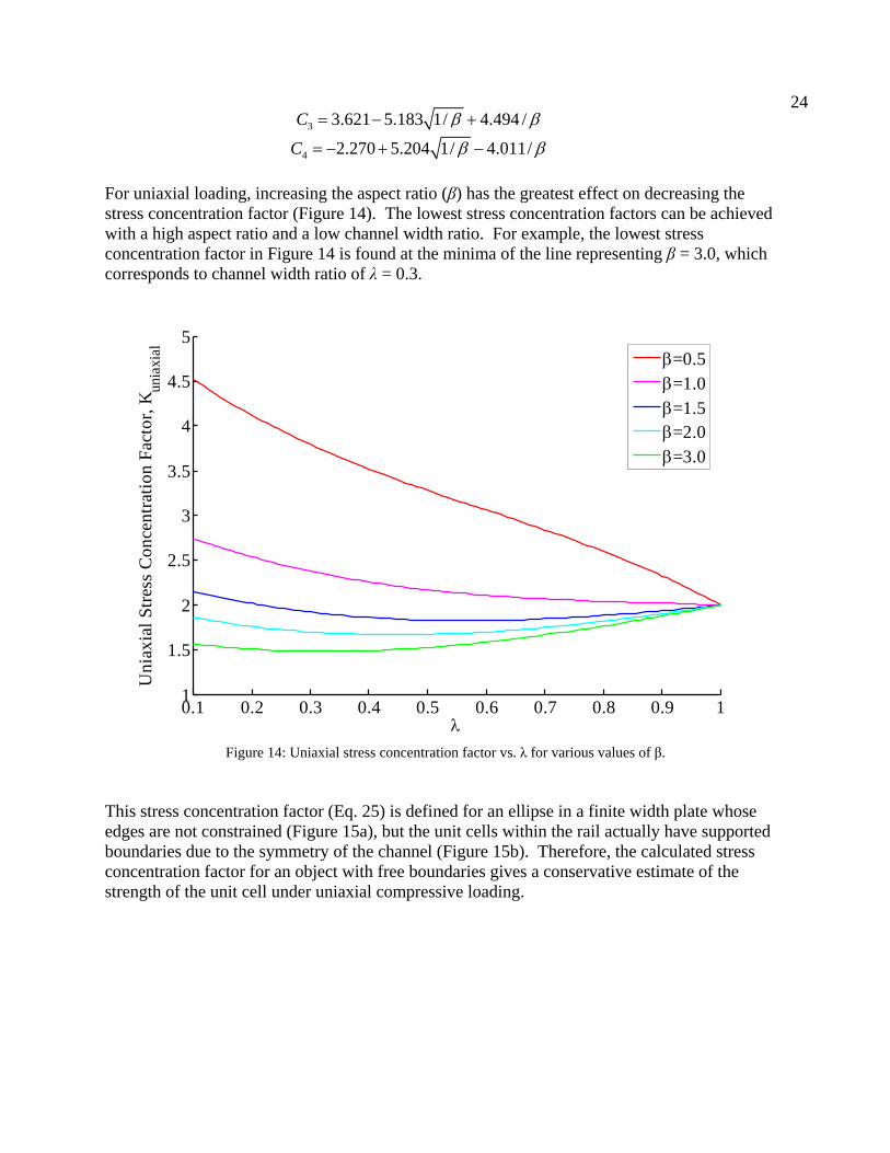
4 2.270 5.204 1/ 4.011/C β β= − + − For uniaxial loading, increasing the aspect ratio (β) has the greatest effect on decreasing the stress concentration factor (Figure 14). The lowest stress concentration factors can be achieved with a high aspect ratio and a low channel width ratio. For example, the lowest stress concentration factor in Figure 14 is found at the minima of the line representing β = 3.0, which corresponds to channel width ratio of λ = 0.3.
0.1 0.2 0.3 0.4 0.5 0.6 0.7 0.8 0.9 11
1.5
2
2.5
3
3.5
4
4.5
5
λ
Uni
axia
l Stre
ss C
once
ntra
tion
Fact
or, K
uni
axia
l
β=0.5β=1.0β=1.5β=2.0β=3.0
Figure 14: Uniaxial stress concentration factor vs. λ for various values of β.
This stress concentration factor (Eq. 25) is defined for an ellipse in a finite width plate whose edges are not constrained (Figure 15a), but the unit cells within the rail actually have supported boundaries due to the symmetry of the channel (Figure 15b). Therefore, the calculated stress concentration factor for an object with free boundaries gives a conservative estimate of the strength of the unit cell under uniaxial compressive loading.
25
a) b)
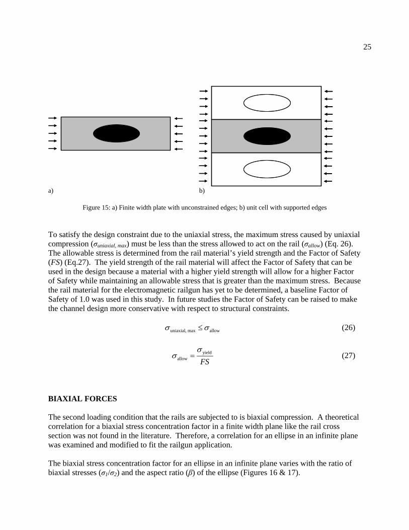
Figure 15: a) Finite width plate with unconstrained edges; b) unit cell with supported edges To satisfy the design constraint due to the uniaxial stress, the maximum stress caused by uniaxial compression (σuniaxial, max) must be less than the stress allowed to act on the rail (σallow) (Eq. 26). The allowable stress is determined from the rail material’s yield strength and the Factor of Safety (FS) (Eq.27). The yield strength of the rail material will affect the Factor of Safety that can be used in the design because a material with a higher yield strength will allow for a higher Factor of Safety while maintaining an allowable stress that is greater than the maximum stress. Because the rail material for the electromagnetic railgun has yet to be determined, a baseline Factor of Safety of 1.0 was used in this study. In future studies the Factor of Safety can be raised to make the channel design more conservative with respect to structural constraints. uniaxial, max allowσ σ≤ (26)
yieldallow FS
σσ = (27)
BIAXIAL FORCES The second loading condition that the rails are subjected to is biaxial compression. A theoretical correlation for a biaxial stress concentration factor in a finite width plane like the rail cross section was not found in the literature. Therefore, a correlation for an ellipse in an infinite plane was examined and modified to fit the railgun application. The biaxial stress concentration factor for an ellipse in an infinite plane varies with the ratio of biaxial stresses (σ1/σ2) and the aspect ratio (β) of the ellipse (Figures 16 & 17).

26
Figure 16: Infinite plate with a single elliptical hole (β=2) subject to biaxial loading
-5 0 50
1
2
3
4
5
6
7
Biaxial stress ratio, σ1 / σ2
Bia
xial
stre
ss c
once
ntra
tion
fact
or, K
bia
xial
σ1 / σ2 = 1/ βσ1 / σ2 = -1/ β2
σ1 / σ2 = 1
σ1 / σ2 = -1
Figure 17: Biaxial stress concentration factor vs. biaxial stress ratio for an ellipse of aspect ratio β =2.0 (Peterson, 1953).
σ2b
a
σ1
..A
Bσ2
ba
σ1
..A
B

27
The maximum stress occurs at either point A or point B of the cross section (Figure 16), depending on the ratio of the stresses (Peterson 1953). For most loading conditions, the highest stresses are at point B. For an ellipse in an infinite plane, this occurs on the following intervals:
12
2
1σσ β
−< and 1
2
1σσ β
> (28)
However, between the two intervals given in Eq. 38, the point of maximum stress occurs at point A:
12
2
1 1σβ σ β−
< < (29)
The maximum stress at points A or B are defined by the following equations (Peterson, 1953):
biaxial max 2 12(1 )
Aσ σ σ
β= + − or biaxial max 1 2(1 2 )
Bσ σ β σ= + − (30)
The stress concentration factor is represented as the ratio of the maximum stress to the greater of the two applied stresses. So, depending on which applied stress has a greater magnitude, the stress concentration factor is defined as following:
biaxial, maxbiaxial
1
Kσ
σ= or biaxial, max
biaxial2
Kσ
σ= (31)
Due to the size of the cooling channel cross section relative to the rail cross section, the above theory (for an infinite plane) must be modified in order to consider a finite width plane (Figure 18). This was achieved by substituting the nominal stress for the applied stresses (Eqs. 32-34). The nominal stresses are calculated from applied stresses on the rail and the unit cell dimensions, as follows:
nominal1 1
22
w bb
σ σ −= (32)
nominal2 2
a ta
σ σ += (33)
nominal nominalbiaxial max 2 1
2(1 )A
σ σ σβ
= + − or nominal nominalbiaxial max 1 2(1 2 )
Bσ σ β σ= + − (34)

28
Figure 18: Biaxial compression acting on an elliptical channel in a unit cell. Since for all of the cases evaluated in this study σ1 / σ2 > 1/β, the point of maximum stress occurred at point B (Figure 16). The allowable stress is defined in the same way as for the uniaxial case (Eq. 27, and the design constraint for this stress condition is: biaxial max biaxial 2Kσ σ= (35) biaxial max allowσ σ≤ (36) 2.4 OPTIMIZATION ROUTINE The cooling channel design was optimized for maximum heat transfer in a unit cell, which corresponds to a minimum thermal resistance (Rfin). This was accomplished by use of a nonlinear constraint minimization routine that was solved with respect to the geometric values of the channel design (a, b, t). First the heat equation and the associated boundary conditions (Eqs. 5-7) that produce Rfin were parameterized. This involved the equations used to determine the heat transfer coefficient (Eq. 10-14; 15-20), so that for any given channel size the heat equation was calculated with the appropriate heat transfer coefficient. The equations of maximum stress acting on the rail were also parameterized in terms of the channel dimensions (Eq. 21-25; 32-36). The optimization was performed using a linearly constrained minimization function in Matlab® to minimize Rfin while meeting both the uniaxial and biaxial constraints of the allowable stress (Appendix 1). Table 1 lists all of the input variables in the optimization.
xyσ2
σ1,nominal
σ1
σ2,nominal
rail cross section width, w
xyσ2
σ1,nominal
σ1
σ2,nominal
xyσ2
σ1,nominal
σ1
σ2,nominal
rail cross section width, w

29
Name Symbol Units Cross section height Hy mm Cross section length Lx mm Number of channels (unit cells) N -- Uniaxial stress σuniaxial MPa Biaxial Stress 1 σbiaxial1 MPa Biaxial Stress 2 σbiaxial 2 MPa Factor of Safety FS 1.0 Rail Material: Thermal conductivity ks W/mK Yield Strength σy MPa Coolant: Thermal conductivity kf W/mK Specific Heat Capacity Cp J/kg-K Density ρ kg/m3 Dynamic viscosity µ N-s/m2
Pump Power totalW& ′ W/m
Table 1: Input variables for optimization function

30
3.0 DESIGN OF AN OPTIMAL CHANNEL FOR A FULL SCALE RAILGUN The general optimization routine described in Chapter 2 can be used to find an optimal cooling channel cross section design for the full size rails of the electromagnetic railgun. The parameters for the U.S. Navy’s Notional Railgun were used as a baseline to for this design (Table 2).
Total energy supplied to the Railgun 150 Mega-Joules Current needed to produce this energy 5.3 Mega-Amperes Inductance gradient in the launch 0.5 Micro-Henries per meter Force on the armature 6.25 Mega-Newtons Uniaxial stress on the rails 386 Mega-Pascals Biaxial stresses on the rails 240 & 180 Mega-Pascals Rail cross section 61 Millimeters by 135 Millimeters Launcher bore size 135 Millimeters by 135 Millimeters
Table 2: Notional Railgun Parameters
3.1 INITIAL DESIGN CHOICES GEOMETRIC CONSTRAINTS In the railgun the electric current is concentrated on the inside surface of the rail resulting in local heating, so cooling that surface is the largest challenge (Figure 5). Therefore the decision was made to find a solution for a single row of channels that are a specified distance from the edge of the rail (Figure 19). The distance between the edge of the rail and the tip of the channel is set at 20 mm because most of the current is carried within 20 millimeters of the surface of the rail (Smith et al, 2005).
Figure 19: Rail with channels 20 mm from edge
20 mm

31
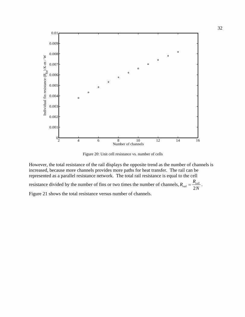
The unit cell size was determined based on the overall rail cross section (135 mm x 61 mm) and the number of channels (N) to be placed in the rail (Ellis et al, 2005). Because cooling channels are only being placed along the height of the rail (135 mm), as the number of cells increased, the height (2a+2t) of the unit cell decreased while the width (61mm) remained constant. MATERIAL SELECTION As calculated from Eqs. (1) and (2), the initial uniaxial compressive load acting on the rails is 386 MPa, which is greater than the yield strength of the standard rail material, ETP copper (310 MPa). Consequently, a stronger material had to be selected just to design a rail, regardless of cooling channel shape. A beryllium copper alloy (UNS C17600 TH04) was selected as the rail material for this study because of its high yield strength (825 MPa) and relatively high thermal conductivity (215 W/m-K), (Davis 2001). POWER CONSTRAINT The total pump power constraint was set at 100 Watts per meter, which was sufficient to assure that there was always turbulent flow in the channels. This power constraint corresponds to channel solutions with Reynolds numbers on the interval 23,000<ReD<71,000. 3.2 RESULTS The optimization routine was performed for a rail cross section with four to fourteen unit cells using the optimization routine explained in Chapter 2 (Appendix 2). Figure 20 shows that as the number of unit cells increased, the optimal unit cell fin resistance increased. It makes sense that smaller unit cells have less heat transfer ability for two reasons: (1) the cell width has become thinner relative to the cell height, leaving less material for conduction and (2) the holes get smaller since they are limited by the stress concentration factor they create.
32
2 4 6 8 10 12 14 160
0.001
0.002
0.003
0.004
0.005
0.006
0.007
0.008
0.009
0.01
Number of channels
Indi
vidu
al fi
n re
sist
ance
(R fi
n) K-m
/ W
Figure 20: Unit cell resistance vs. number of cells However, the total resistance of the rail displays the opposite trend as the number of channels is increased, because more channels provides more paths for heat transfer. The rail can be represented as a parallel resistance network. The total rail resistance is equal to the cell
resistance divided by the number of fins or two times the number of channels,2
cellrail
RRN
= .
Figure 21 shows the total resistance versus number of channels.

33
2 4 6 8 10 12 14 160
0.5
1
1.5
2
2.5
3
3.5
4
4.5
5 x 10⁻⁴
Number of channels
Tota
l rai
l res
ista
nce
K-m
/ W
Figure 21: Total Resistance vs. number of channels. The power constraint also played a role in increasing Rfin with an increasing number of channels. As the number of channels increased, the amount of pump power per channel decreased. This caused the mean fluid velocity to decrease. The decrease in mean fluid velocity and hydraulic diameter caused a lower Reynolds number. This in turn lowered the Nusselt number which lowered the heat transfer coefficient. Figure 22 shows that the heat transfer coefficient as a function of the number of channels.

34
2 4 6 8 10 12 14 160
0.5
1
1.5
2
2.5
3 x 10⁴
Number of channels
Hea
t tra
nsfe
r coe
ffic
ient
(h) W
/ m2 -K
Figure 22: Heat transfer coefficient vs. number of cells.
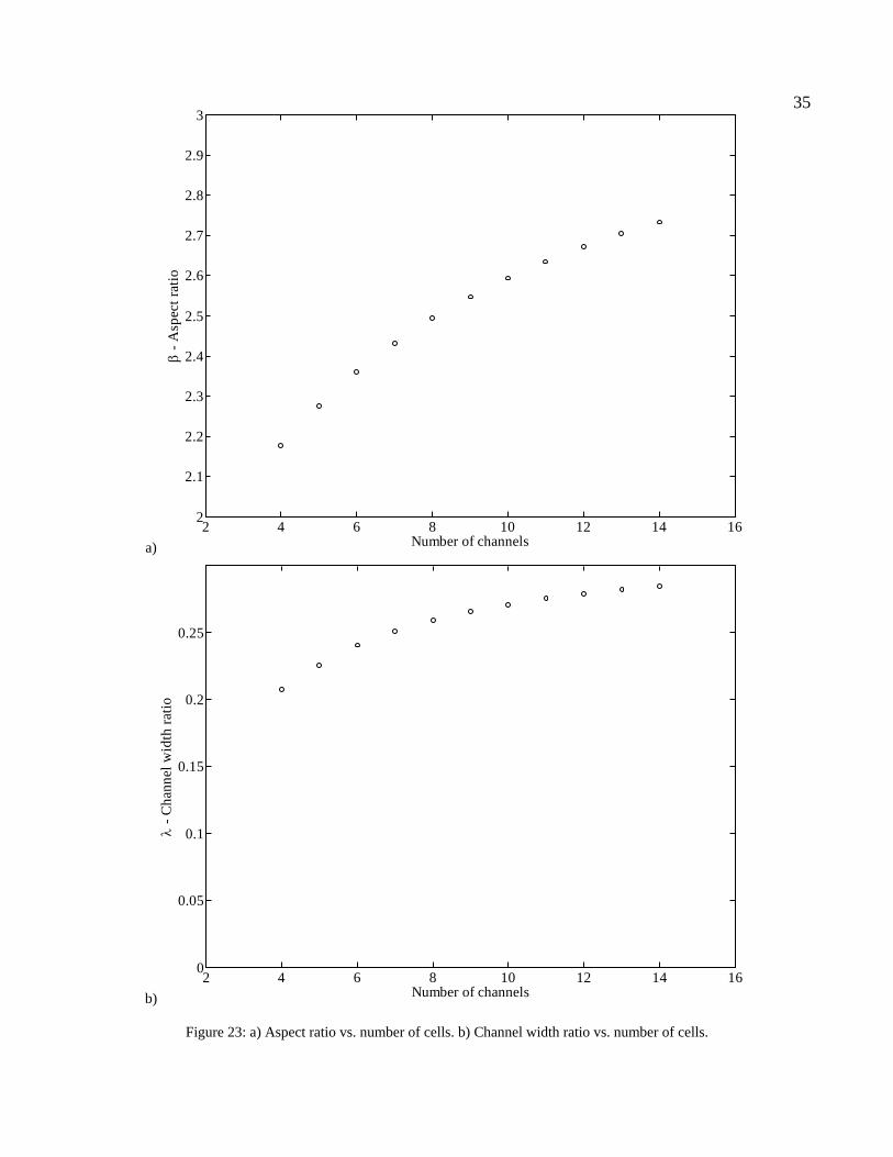
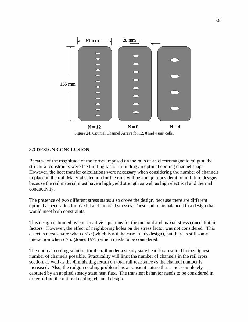
As the number of unit cells increased, the aspect ratio and the channel width ratio (a/(t+a)) increased as well. Figure 23a shows the aspect ratio of the channel versus number of channels, and Figure 23b shows the channel width ratio versus number of channels. In general, as N increased, the optimal ellipse became longer and had more area between each channel relative to the unit cell size. The aspect ratio of the channel cross section changed as the number of unit cells increased because all of the parameters of the unit cell were not scaled to the number of unit cells. As the number of channels increased, the cell height got smaller but the cell width stayed the same. This caused the ratio of biaxial stresses to be different, and consequently a different set of geometric parameters gave an optimal solution where both the uniaxial and biaxial maximum strength constraints were met. Figure 24 shows the optimal channel design for four, eight and twelve channels in a rail.
35
a)2 4 6 8 10 12 14 16
2
2.1
2.2
2.3
2.4
2.5
2.6
2.7
2.8
2.9
3
Number of channels
β - A
spec
t rat
io
b)2 4 6 8 10 12 14 16
0
0.05
0.1
0.15
0.2
0.25
Number of channels
λ - C
hann
el w
idth
ratio
Figure 23: a) Aspect ratio vs. number of cells. b) Channel width ratio vs. number of cells.
36
Figure 24: Optimal Channel Arrays for 12, 8 and 4 unit cells. 3.3 DESIGN CONCLUSION Because of the magnitude of the forces imposed on the rails of an electromagnetic railgun, the structural constraints were the limiting factor in finding an optimal cooling channel shape. However, the heat transfer calculations were necessary when considering the number of channels to place in the rail. Material selection for the rails will be a major consideration in future designs because the rail material must have a high yield strength as well as high electrical and thermal conductivity. The presence of two different stress states also drove the design, because there are different optimal aspect ratios for biaxial and uniaxial stresses. These had to be balanced in a design that would meet both constraints. This design is limited by conservative equations for the uniaxial and biaxial stress concentration factors. However, the effect of neighboring holes on the stress factor was not considered. This effect is most severe when t < a (which is not the case in this design), but there is still some interaction when t > a (Jones 1971) which needs to be considered. The optimal cooling solution for the rail under a steady state heat flux resulted in the highest number of channels possible. Practicality will limit the number of channels in the rail cross section, as well as the diminishing return on total rail resistance as the channel number is increased. Also, the railgun cooling problem has a transient nature that is not completely captured by an applied steady state heat flux. The transient behavior needs to be considered in order to find the optimal cooling channel design.
20 mm
135 mm
61 mm
N = 12 N = 8 N = 4
20 mm
135 mm
61 mm
N = 12 N = 8 N = 4
37
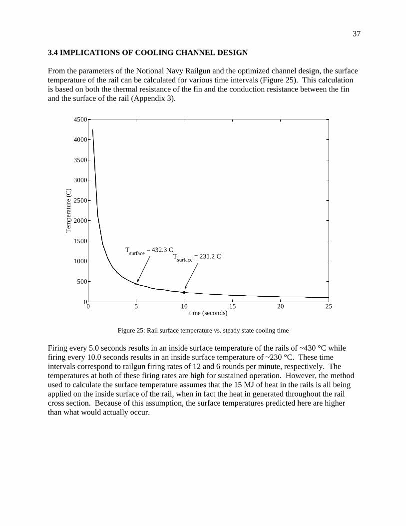
3.4 IMPLICATIONS OF COOLING CHANNEL DESIGN From the parameters of the Notional Navy Railgun and the optimized channel design, the surface temperature of the rail can be calculated for various time intervals (Figure 25). This calculation is based on both the thermal resistance of the fin and the conduction resistance between the fin and the surface of the rail (Appendix 3).
0 5 10 15 20 250
500
1000
1500
2000
2500
3000
3500
4000
4500
time (seconds)
Tem
pera
ture
(C)
Tsurface = 432.3 C Tsurface = 231.2 C
Figure 25: Rail surface temperature vs. steady state cooling time
Firing every 5.0 seconds results in an inside surface temperature of the rails of ~430 °C while firing every 10.0 seconds results in an inside surface temperature of ~230 °C. These time intervals correspond to railgun firing rates of 12 and 6 rounds per minute, respectively. The temperatures at both of these firing rates are high for sustained operation. However, the method used to calculate the surface temperature assumes that the 15 MJ of heat in the rails is all being applied on the inside surface of the rail, when in fact the heat in generated throughout the rail cross section. Because of this assumption, the surface temperatures predicted here are higher than what would actually occur.
38
4.0 EXPERIMENTAL CONFIGURATION 4.1 SCALED PARAMETERS The proposed rails in the full size notional Navy railgun will be 10 to 12 meters long with a cross section of 61mm by 135 mm. It was not feasible to fabricate or heat even a small length of a rail with this cross section, so the rail size was scaled down in order for a laboratory model to be built and tested. The experimental rails were manufactured out of 18-inch long pieces of 1-inch by 2-inch Electrolytic Tough Pitch (ETP) Copper, the current standard material for railgun testing because of its high electrical and thermal conductivity (388 W/mK, Davis, 2001). The size reduction in the rail cross section corresponds to a scaling factor of approximately 2.5. Because of the relatively low yield strength of ETP Copper (310 MPa) relative to the uniaxial stress for full size rails, the forces used in designing the scaled down rails were reduced as shown in Table 3. These scaled forces are computed based on a current of 1 MA, which is on the same order of magnitude as the current Army railgun design.
Original rail Scaled Rail σuniaxial = 386 MPa σuniaxial = 110 MPa σbiaxial 1 = 165 MPa σbiaxial 1 = 47.1 MPa σbiaxial 2 = 240 MPa σbiaxial 2 = 68.6 MPa
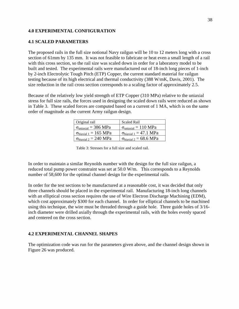
Table 3: Stresses for a full size and scaled rail. In order to maintain a similar Reynolds number with the design for the full size railgun, a reduced total pump power constraint was set at 50.0 W/m. This corresponds to a Reynolds number of 58,600 for the optimal channel design for the experimental rails. In order for the test sections to be manufactured at a reasonable cost, it was decided that only three channels should be placed in the experimental rail. Manufacturing 18-inch long channels with an elliptical cross section requires the use of Wire Electron Discharge Machining (EDM), which cost approximately $300 for each channel. In order for elliptical channels to be machined using this technique, the wire must be threaded through a guide hole. Three guide holes of 3/16-inch diameter were drilled axially through the experimental rails, with the holes evenly spaced and centered on the cross section. 4.2 EXPERIMENTAL CHANNEL SHAPES The optimization code was run for the parameters given above, and the channel design shown in Figure 26 was produced.
39
a 0.003281 m t 0.005189 m b 0.006050 m
Figure 26: Optimized Design for the experimental rail
The thermal and structural aspects of this design were then independently verified. The structural aspect of the design was verified using Finite Element Analysis (Chapter 5) while the heat transfer component of the design was verified by physical testing. In order to select channel shapes for test, Rfin is graphed with respect to b, with a and t set constant for the values found in the optimization (Figure 27).
2 4 6 8 10 12x 10-3
4
4.1
4.2
4.3
4.4
4.5
4.6 x 10⁻³
half-length "b" (m)
Rfin
( K
/ W
) Point 3:Optimal solution for heat transfer
Point 2:Optimal solution with structural constraints
Point 1:Non-optimized solution
Figure 27: Fin resistance vs. ellipse half length (b).
t
2t
2b
2a
t
2t
2b
2a

40
The optimal solution for heat transfer occurs at the minima of the curve, at point 3. However, the optimization code achieves an increased Rfin when the design is limited by structural constraints rather than heat transfer ability (point 2). The channel shapes associated with both of these points will be tested, as well as the channel design with a half length at point 1 (Table 4).
Rail 1 Rail 2 Rail 3 b1 = 0.354 in b2 = 0.476 in b3 = 0.598 in Rfin = 0.004145 K/W Rfin = 0.004052 K/W Rfin = 0.004028 K/W Non-optimized channels
Channels optimized with structural constraints
Channels optimized without structural constraints
ReD=56,600 ReD=58,600 ReD=58,700
Table 4: Experimental Rail Parameters

41
5.0 FINITE ELEMENT ANALYSIS OF DESIGN The structural aspect of the channel design was verified by comparing stress concentrations factors from the finite element analysis software package (I-DEAS) to stress concentration factors that were produced from the analytical equations. Stress concentration factors were compared for various geometries and loading conditions—from general cases found in the literature to the specific rail design produced by the optimization code. For all of the I-DEAS modeling, a quarter of a single unit cell was used to represent the rail cross section. A quarter section can be analyzed as representative of the whole rail because of the symmetry of the unit cell and the assumption of uniform stresses acting on the faces of the rail (Figure 28).
Figure 28: Quarter unit cell with forces and constraints shown. The rail cross sections were modeled in I-DEAS using a two dimensional shell mesh of elements in plane strain. A shell mesh in plane strain assumes that all deformation (and consequently all strain) occurs within the plane being modeled (Shih, 2002). The assumption that the part cannot deform out of the plane is valid for very thick objects, and the dimensions of a rail are such that the rail can be considered to have infinite thickness. There will be edge effects at the breach end of the rail, but this problem will likely be remedied by other structural constraints and this case was not considered in this design. According to convention, the parts were modeled in the xy plane (rail cross section), and there is no strain in the z direction (along the length of the rail). 5.1 UNIAXIAL STRESS CONCENTRATION FACTOR FROM I-DEAS The first subject for I-DEAS modeling was a general quarter unit cell with a circular hole in it in uniaxial tension (Figure 29).
y
x
y
x

42
Figure 29: Quarter of a unit cell with a circular hole in uniaxial compression, with stress concentration factors shown.
The I-DEAS solution displays the stresses that occur in each element in the model, and from this solution the maximum principal stress can be found along with the location of this stress on the model. The uniaxial stress concentration factor was determined by finding the ratio of the highest maximum principal stress on the model to the applied stress (Eq. 37). For all uniaxial cases, the applied stress was unity, so the stress concentration factor was effectively the maximum principal stress. Also, in I-DEAS compression has a negative sign, so the maximum principal stress in the model is actually the most negative number displayed in the results which corresponds to the blue region on Figure 28. When compared to the analytical stress concentration factor, the difference between the I-DEAS and analytical stress concentration factors in the first model was 0.04% (Eq. 37; Appendix 4).
max principaluniaxial
applied
Kσσ
= (37)
After mesh independence was verified and the most accurate element shape was found (3 point triangle), the dimensions of the plate were changed. As the plate got shorter in the direction of the loading relative to the hole size, the numerical results began to diverge from the analytical stress concentration factor. Since the equation for the uniaxial stress concentration factor does not include the plate dimension in the direction of the loading, it can be assumed that this equation does not account for end effects in this direction. The applicability of the analytical expression breaks down under these conditions. After the numerical stress concentration factors for a circular hole and their relationship to the theory were well understood, the stress concentration factor for an ellipse in uniaixial loading was explored. Ellipses of aspect ratios of 0.5 < β < 3 were examined and all of the stress concentration factors were close to the analytical results (Appendix 4). However, the stress concentration factors determined analytically were consistently higher than the stress
0.154
-4.349
0.00.154
-4.349
0.0
Stre
ss C
once
ntra
tion
Fact
or, K

43
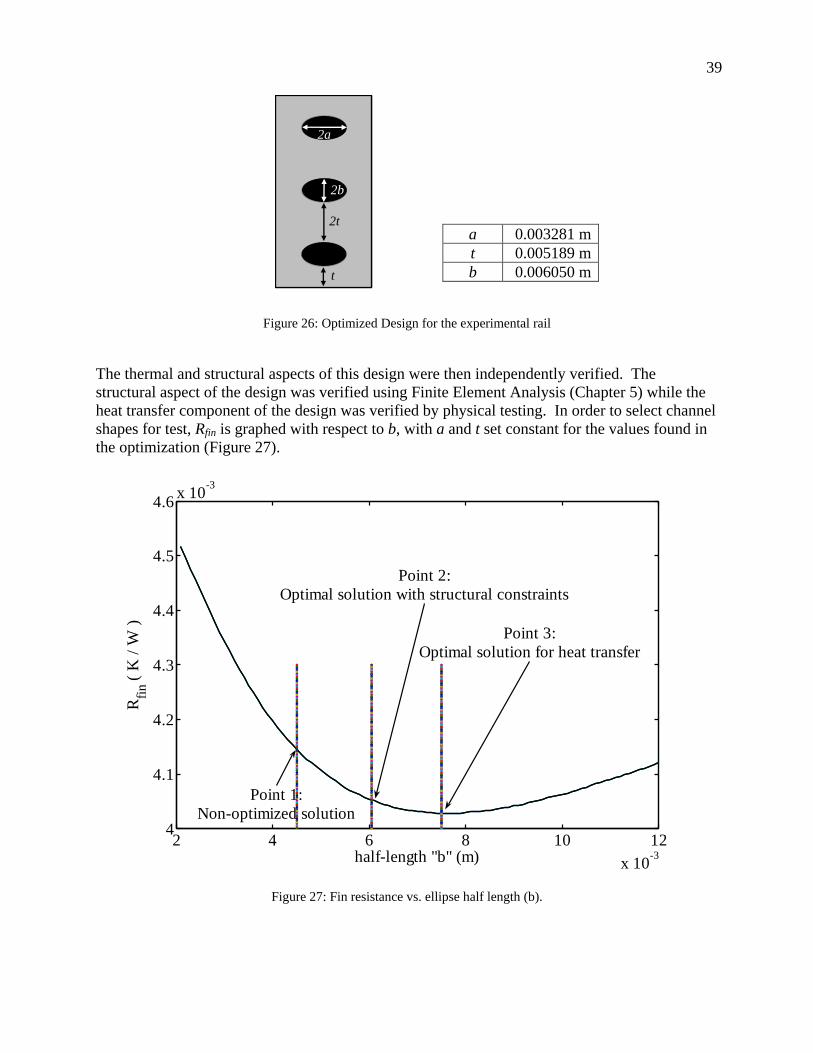
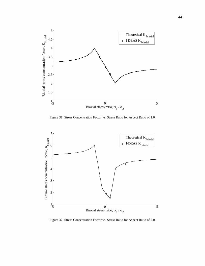
concentration factors found numerically. This is because the analytical equation was derived using the assumptions of plane stress rather than plane strain (Young and Budynas, 2002). Plane stress assumes that there is strain but no stress perpendicular to the plane, and this assumption is valid for thin plates. Conversely, plane strain models an object with infinite thickness under the assumption that there is stress but no strain perpendicular to the plane. The I-DEAS modeling used elements in plane strain because these assumptions more closely match the physical reality of rails in a railgun even though the analytical equations were based on plane stress. Because plane stress gives a more conservative but still reasonable stress concentration factor, it is acceptable to use this analytical theory in the optimization code. 5.2 BIAXIAL STRESS CONCENTRATION FACTOR FROM I-DEAS The correlation between biaxial stress concentration factors was investigated next. Since the analytical solution exists only for an infinite plate, assumptions were made to modify the theory for a finite plate (see section 2.3). Because of these theoretically sound but untested assumptions and the added variable of biaxial stress ratio, the biaxial stress concentration factor correlation proved to be much harder to verify than the uniaxial correlation, which was not modified in any way. The first biaxial model analyzed was a very large unit cell with a very small hole (hole diameter 1% of unit cell length and width) that closely approximated the infinite model in the literature (Figure 30). The correlation of stress concentration factors for an aspect ratio of 1.0 and 2.0 were almost exact (Figure 31 & 32). The correlation started to break down for an aspect ratio of 3.0 (Figure 33). The results still followed the trend of the analytical curve, but all the stress concentration factors were lower than predicted (Appendix 5). This can be attributed in part to the different stress theories used in I-DEAS (plane strain) and the literature (plane stress).
Figure 30: Approximation of an infinite plane with an elliptical hole with aspect ratio of three.
-0.878
-2.07
Stre
ss C
once
ntra
tion
Fact
or, K
44
-5 0 51
1.5
2
2.5
3
3.5
4
4.5
5
Biaxial stress ratio, σ1 / σ2
Bia
xial
stre
ss c
once
ntra
tion
fact
or, K
bia
xial Theoretical K biaxial
I-DEAS K biaxial
Figure 31: Stress Concentration Factor vs. Stress Ratio for Aspect Ratio of 1.0.
-5 0 51
2
3
4
5
6
7
Biaxial stress ratio, σ1 / σ2
Bia
xial
stre
ss c
once
ntra
tion
fact
or, K
bia
xial Theoretical K biaxialI-DEAS K biaxial
Figure 32: Stress Concentration Factor vs. Stress Ratio for Aspect Ratio of 2.0.
45
-5 0 51
2
3
4
5
6
7
8
9
Biaxial stress ratio, σ1 / σ2
Bia
xial
stre
ss c
once
ntra
tion
fact
or, K
bia
xial Theoretical K biaxial
I-DEAS K biaxial
Figure 33: Stress Concentration Factor vs. Stress Ratio for Aspect Ratio of 3.0. A unit cell of the dimensions that were found using the experimental parameters in the optimization code was next modeled under various stress ratios (Figure 34). The stress concentration factors from these test cases were compared to analytical values for stress concentration factors that accounted for the finite width of the unit cell (Appendix 6). The stress concentration factors from I-DEAS followed the general trend of the analytical equations, but the results appeared to be shifted to the right (Figure 35). However, in the region of interest for this project (biaxial stress ratio between 0.25 and 1.0), the correlation between numerical and analytical results was very close, and the analytical equations provided a conservative estimate of the stress concentration factor.
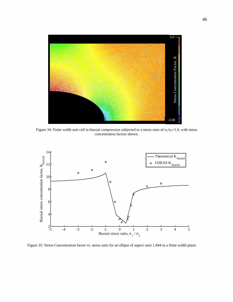
46
Figure 34: Finite width unit cell in biaxial compression subjected to a stress ratio of σ1/σ2=1.0, with stress concentration factors shown.
-5 -4 -3 -2 -1 0 1 2 3 4 52
4
6
8
10
12
14
Biaxial stress ratio, σ1 / σ2
Bia
xial
stre
ss c
once
ntra
tion
fact
or, K
bia
xial Theoretical K biaxial
I-DEAS K biaxial
Figure 35: Stress Concentration factor vs. stress ratio for an ellipse of aspect ratio 1.844 in a finite width plane.
-7.16
0.0
Stre
ss C
once
ntra
tion
Fact
or, K
-3.08

47
5.3 FINITE ELEMENT ANALYSIS CONCLUSION The finite element analysis performed in this study is sufficient to verify both the uniaxial and biaxial stress concentration factor correlations used in the optimization study. The uniaxial correlation was verified when there was sufficient space between the edge of the plate and the channel, and the biaxial correlation was accurate for shapes with low aspect ratios (β < 3.0) and for stress ratios of -0.75< σ1/σ2 <1.0. All of these qualifications on the use of the stress concentration factors fall within the range of use for railgun cooling channels, so the optimization routine can be considered sound and conservative with respect to the structural constraints.

48
6.0 EXPERIMENTAL VERIFICATION OF HEAT TRANSFER PERFORMANCE UNDER STEADY STATE CONDITIONS As explained in Section 3.2, three rails with different channel shapes were tested. The channels have constant values of a and t, and each rail has channels with a different value of b (Figure 36). In Figure 35 the four small holes in each rail are taps for attaching the manifold. Each rail was heated and cooled under steady state conditions, with its heat transfer performance measured in terms of thermal resistance of a fin (Rfin).
Figure 36: Three experimental channel designs 6.1 EXPERIMENTAL SET-UP The heat transfer capability of the cooling channel design was tested by cooling a rail while a constant heat flux was applied to its surface using a Kapton flexible heater that supplied 1000 Watts to the experimental rail (Figure 37).

49
Figure 37: Kapton heater applied to rail surface In order to achieve good contact between the heater and the rails, several safeguards were employed. First, thermal grease was applied between the bar and the heater. Then the bar and heater were placed in a containment piece made of the composite G-10 (Figure 38). G-10 was chosen because it is fire retardant and a reasonable insulator (Appendix 7). The top and bottom piece of the containment were bolted together and a piece of rubber the size of the heater was placed under the heater to further ensure good contact between the heater and the bar at all points along the length of the bar.
Figure 38: G-10 Containment
Water at 20° C (T∞) was pumped through the system using a Merlin Series Thermo NESLAB Chiller. This chiller was able to provide an overall flow rate (V& ) of approximately 18 liters per

50
minute (LPM). Upon exiting the chiller, the flow was divided into three separate lines for the three cooling channels. With the flow divided and due to the losses between the chiller and the flowmeters, a maximum flow rate between 5.5 and 6.0 LPM was achieved when all three lines of the system were open. A flow rate of 6.0 LPM corresponds to a Reynolds number of 75,000 for the optimized channels in Rail #2. In order to pipe the water from circular tubing coming from the chiller into the elliptical channels, a manifold device was designed (Figure 39a). Copper tubing was soldered into one end of the manifold, and then elliptical holes that were bigger then all three experimental channel sizes were milled into the other side of the manifold. Because the manifold was copper, it was necessary to insulate it from the rails. This was accomplished using a polyethylene spacer block with a rubber gasket on each side (Figure 39b).
Figure 39: a) Manifold device
Figure 39: b) Manifold device connected to the rail.
51
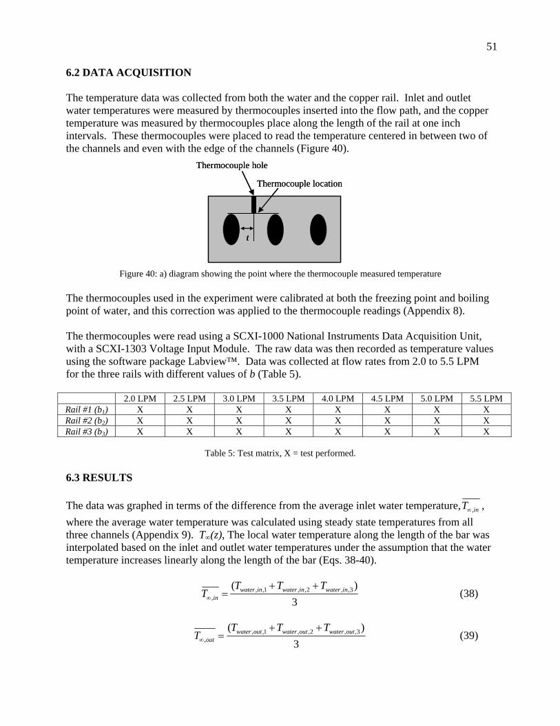
6.2 DATA ACQUISITION The temperature data was collected from both the water and the copper rail. Inlet and outlet water temperatures were measured by thermocouples inserted into the flow path, and the copper temperature was measured by thermocouples place along the length of the rail at one inch intervals. These thermocouples were placed to read the temperature centered in between two of the channels and even with the edge of the channels (Figure 40).
Figure 40: a) diagram showing the point where the thermocouple measured temperature The thermocouples used in the experiment were calibrated at both the freezing point and boiling point of water, and this correction was applied to the thermocouple readings (Appendix 8). The thermocouples were read using a SCXI-1000 National Instruments Data Acquisition Unit, with a SCXI-1303 Voltage Input Module. The raw data was then recorded as temperature values using the software package Labview™. Data was collected at flow rates from 2.0 to 5.5 LPM for the three rails with different values of b (Table 5).
2.0 LPM 2.5 LPM 3.0 LPM 3.5 LPM 4.0 LPM 4.5 LPM 5.0 LPM 5.5 LPM Rail #1 (b1) X X X X X X X X Rail #2 (b2) X X X X X X X X Rail #3 (b3) X X X X X X X X
Table 5: Test matrix, X = test performed. 6.3 RESULTS The data was graphed in terms of the difference from the average inlet water temperature, ,inT∞ , where the average water temperature was calculated using steady state temperatures from all three channels (Appendix 9). T∞(z), The local water temperature along the length of the bar was interpolated based on the inlet and outlet water temperatures under the assumption that the water temperature increases linearly along the length of the bar (Eqs. 38-40).
, ,1 , ,2 , ,3,
( )3
water in water in water inin
T T TT∞
+ += (38)
, ,1 , ,2 , ,3,
( )3
water out water out water outout
T T TT∞
+ += (39)
t
Thermocouple location
Thermocouple hole
t
Thermocouple location
Thermocouple hole

52
, ,,
( )( ) out in
in
T TT z T z
L∞ ∞
∞ ∞
−= + (40)
As the cooling fluid enters the channel, both thermal and velocity boundary layers begin to develop along the surface of the channel. These boundary layers grow down the length of the channel until they eventually meet in the center of the channel, at which point the flow is considered to be fully developed. Before this point, the flow is in the entry region, and the length of this region is called the entry length. The velocity and thermal entry lengths are usually different, and both are a function of the fluid and channel properties (Incropera and DeWitt, 2002). The thermally fully developed region is important in analyzing these results because when the flow is thermally fully developed, both the temperature difference between the fluid and the surface and the convective heat transfer coefficient are constant. Therefore, data points in this region can be compared to the predicted values calculated in the optimization sequence, because the heat transfer coefficient used in the optimization sequence was based on fully developed flow conditions. In the fully developed region the measured rail temperature should change at the same rate as the fluid temperature (with respect to z). Under this assumption, a line parallel to the fluid temperature was applied to the rail temperature data at the corresponding flow rate, and the data points that fit the slope of this line were designated as the fully developed region (Figures 41-43). These data points were chosen by visual inspection, but because of the small number of data points and the distance between them it is likely that a statistical correlation, such as a least squares fit, would yield the same results. In an ideal experiment the fully developed region should extend to the end of the rail, but this trend is not observed due to heat losses and changes in the flow pattern near the ends of the rail. As the channel size increases from rails #1 to #3, the length required for the flow to become fully developed increases, and the size of fully developed region decreases (Table 6; Figures 41-43; Appendix 10). This is as predicted, because the general calculation of thermal entry length (zfd,
T) is a function of the hydraulic diameter of the channel for turbulent flow (Eq. 41; Incropera and DeWitt, 2002).
, T10 60fd
H
zD
< < (41)
Flow rate (LPM) 2.0 2.5 3.0 3.5 4.0 4.5 5.0 5.5
Rail #1 7 - 13 6 - 13 6 - 13 6 - 13 6 - 13 5 - 13 5 - 13 5 - 13 Rail #2 9 - 12 9 - 13 8 - 15 8 - 15 9 - 15 9 - 15 9 - 15 9 - 15 Rail #3 12 - 15 10 - 15 10 - 15 10 - 15 9 - 15 8 - 15 8 - 15 8 - 15
Table 6: Thermally fully developed regions (in z) for given flow rates and channel geometries.
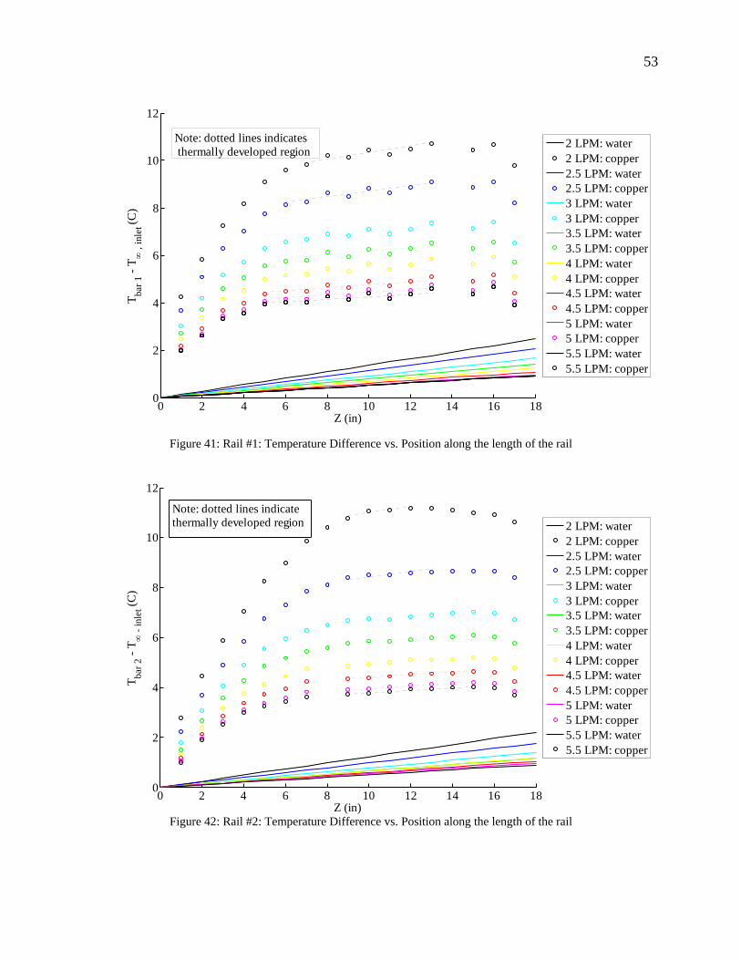
53
0 2 4 6 8 10 12 14 16 180
2
4
6
8
10
12
Z (in)
T bar 1
- T ∞
, in
let (C
)2 LPM: water2 LPM: copper2.5 LPM: water2.5 LPM: copper3 LPM: water3 LPM: copper3.5 LPM: water3.5 LPM: copper4 LPM: water4 LPM: copper4.5 LPM: water4.5 LPM: copper5 LPM: water5 LPM: copper5.5 LPM: water5.5 LPM: copper
Note: dotted lines indicates thermally developed region
Figure 41: Rail #1: Temperature Difference vs. Position along the length of the rail
0 2 4 6 8 10 12 14 16 180
2
4
6
8
10
12
Z (in)
T bar 2
- T ∞
- in
let (C
)
2 LPM: water2 LPM: copper2.5 LPM: water2.5 LPM: copper3 LPM: water3 LPM: copper3.5 LPM: water3.5 LPM: copper4 LPM: water4 LPM: copper4.5 LPM: water4.5 LPM: copper5 LPM: water5 LPM: copper5.5 LPM: water5.5 LPM: copper
Note: dotted lines indicatethermally developed region
Figure 42: Rail #2: Temperature Difference vs. Position along the length of the rail
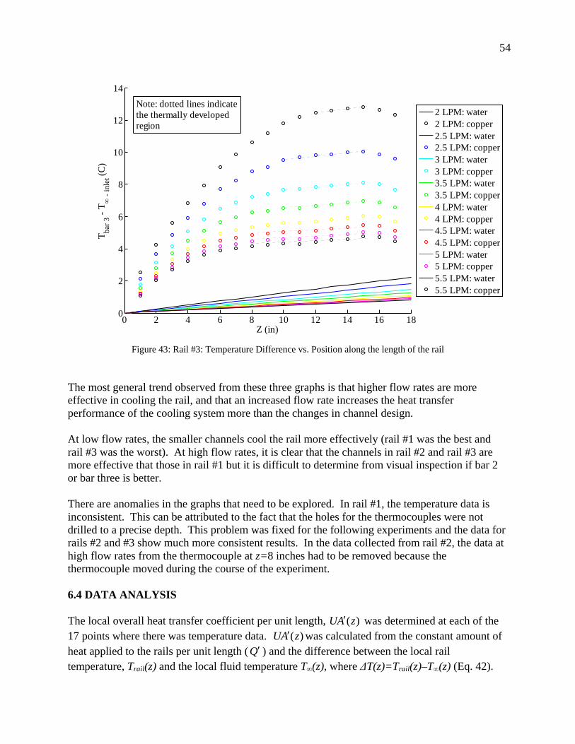
54
0 2 4 6 8 10 12 14 16 180
2
4
6
8
10
12
14
Z (in)
T bar 3
- T ∞
- in
let (C
)2 LPM: water2 LPM: copper2.5 LPM: water2.5 LPM: copper3 LPM: water3 LPM: copper3.5 LPM: water3.5 LPM: copper4 LPM: water4 LPM: copper4.5 LPM: water4.5 LPM: copper5 LPM: water5 LPM: copper5.5 LPM: water5.5 LPM: copper
Note: dotted lines indicatethe thermally developedregion
Figure 43: Rail #3: Temperature Difference vs. Position along the length of the rail
The most general trend observed from these three graphs is that higher flow rates are more effective in cooling the rail, and that an increased flow rate increases the heat transfer performance of the cooling system more than the changes in channel design. At low flow rates, the smaller channels cool the rail more effectively (rail #1 was the best and rail #3 was the worst). At high flow rates, it is clear that the channels in rail #2 and rail #3 are more effective that those in rail #1 but it is difficult to determine from visual inspection if bar 2 or bar three is better. There are anomalies in the graphs that need to be explored. In rail #1, the temperature data is inconsistent. This can be attributed to the fact that the holes for the thermocouples were not drilled to a precise depth. This problem was fixed for the following experiments and the data for rails #2 and #3 show much more consistent results. In the data collected from rail #2, the data at high flow rates from the thermocouple at z=8 inches had to be removed because the thermocouple moved during the course of the experiment. 6.4 DATA ANALYSIS The local overall heat transfer coefficient per unit length, ( )UA z′ was determined at each of the 17 points where there was temperature data. ( )UA z′ was calculated from the constant amount of heat applied to the rails per unit length (Q′ ) and the difference between the local rail temperature, Trail(z) and the local fluid temperature T∞(z), where ∆T(z)=Trail(z)–T∞(z) (Eq. 42).
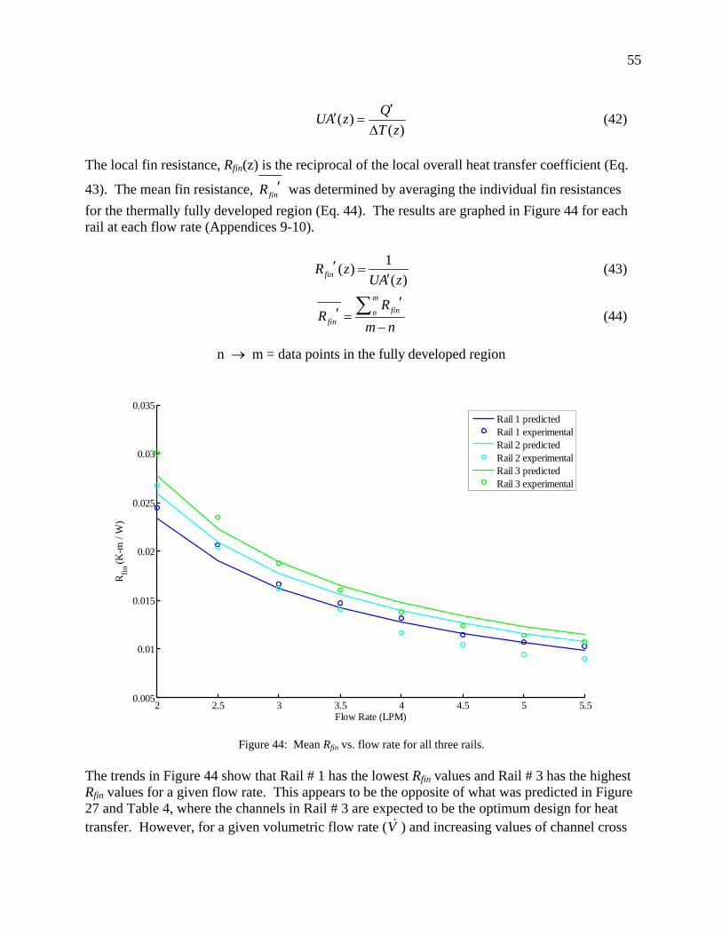
55
( )( )
QUA zT z′
′ =∆
(42)
The local fin resistance, Rfin(z) is the reciprocal of the local overall heat transfer coefficient (Eq.
43). The mean fin resistance, finR ′ was determined by averaging the individual fin resistances for the thermally fully developed region (Eq. 44). The results are graphed in Figure 44 for each rail at each flow rate (Appendices 9-10).
1( )( )finR z
UA z′ =
′ (43)
m
finnfin
RR
m n
′′ =
−∑ (44)
n m = data points in the fully developed region→
2 2.5 3 3.5 4 4.5 5 5.50.005
0.01
0.015
0.02
0.025
0.03
0.035
Rfin
(K-m
/ W
)
Flow Rate (LPM)
Rail 1 predictedRail 1 experimentalRail 2 predictedRail 2 experimentalRail 3 predictedRail 3 experimental
Figure 44: Mean Rfin vs. flow rate for all three rails.
The trends in Figure 44 show that Rail # 1 has the lowest Rfin values and Rail # 3 has the highest Rfin values for a given flow rate. This appears to be the opposite of what was predicted in Figure 27 and Table 4, where the channels in Rail # 3 are expected to be the optimum design for heat transfer. However, for a given volumetric flow rate (V& ) and increasing values of channel cross

56
sectional area (Aellipse), the mean fluid velocity (Um) decreases (Eq. 17). To accurately compare the performance of the three rail designs Rfin must be analyzed with respect to Um instead of volumetric flow rate (Figure 45; Appendix 10). For a given mean fluid velocity (e.g. 0.8 m/s), the lowest values of Rfin correspond to Rail # 3 and the highest values correspond to Rail # 1.
0.4 0.6 0.8 1 1.2 1.4 1.6 1.8 20.005
0.01
0.015
0.02
0.025
0.03
0.035
Rfin
(K-m
/ W
)
Mean Fluid Velocity, Um (m/s)
Rail 1 predictedRail 1 experimentalRail 2 predictedRail 2 experimentalRail 3 predictedRail 3 experimental
Um = 0.8 m/s
Figure 45: Mean Rfin vs. mean fluid velocity for all three rails. As shown in Figures 44 and 45, the Rfin data followed the predicted Rfin values to a degree that this experiment can be considered to validate the theory used in the optimization routine. The experimental Rfin values follow the general trend of the predicted results, and all the experimental values are within 20 % of the predicted values. In the cases where the actual Rfin values were lower than predicted, this can be attributed to the fact that the heat does not actually flow unidirectionally as assumed in the optimization. Because heat actually flows three dimensionally, there are more paths for the heat to dissipate than assumed. Another reason for lower Rfin values than predicted is that while attempts were made to insulate the rail, no material is truly nonconductive, so heat is lost to the surroundings. When the surroundings are not considered in the calculations, the heat lost makes the Rfin values lower than they should be.

57
7.0 TRANSIENT CONSIDERATIONS Although the optimization used in this study was based on a steady state analysis, the railgun cooling problem is inherently transient in nature. Further optimization and design will need to be done with transient assumptions, but as a starting point, this steady state design was tested to evaluate its transient cooling ability. 7.1 FINITE DIFFERENCE MODEL OF THE TRANSIENT THERMAL RESPONSE The transient problem was modeled by analyzing a half unit cell broken into nodes and elements (Figure 46). The heat transfer was modeled using an implicit 1-D finite difference solution.
Figure 46: Unit cell half section, with nodes and elements identified An energy balance is performed on each element. Figure 47a shows heat flowing into node i from nodes i-1 and i+1 as well as from the water in the channel (T∞). Because of the symmetry of a unit cell, no heat crosses the upper unit cell boundary, so the top of the unit cell can be represented as being insulated. Several geometric parameters need to be defined to solve this problem; they are shown in Figure 47b.
a) b) Figure 47: Single node in contact with the cooling channel, with a) nodal temperatures and heat terms; b) geometric
parameters defined
An array was developed for yj, yf and LS; where LS is the length exposed to convection, yj is the right-hand boundary of the element, and yf in the average height of the element. The variables defined above can be substituted into the general heat equation for a transient system (Eq. 45).
1 2 i-1 i1 2 i-1 i
T∞
iT1iT − 1iT +
1i iq − →
iq∞→
1i iq + →
T∞
iT1iT − 1iT +
1i iq − →
iq∞→
1i iq + →
ify
1ijy
− ijy
iLS
x∆
ify
1ijy
− ijy
iLS
x∆

58
The equation is then manipulated into the form shown in Eq. 47, with the corresponding coefficients a, b, c and d.
( ) ( ) 1
1 1 1 1 11 11 1i
i i
n n n n n nf i i n ni i i i
j i i j
Cp y x T T T T T Tk y h LS T T k yt x x
ρ+
+ + + + ++ +− +
∞
⋅ ⋅ ⋅∆ − ⎛ ⎞ ⎛ ⎞− −= ⋅ + ⋅ − + ⋅⎜ ⎟ ⎜ ⎟∆ ∆ ∆⎝ ⎠ ⎝ ⎠
(45)
ss
2 Cpxtk
Fo s
⋅⋅∆∆⋅
=ρ
(46)
1 1 1
1 1n n n
i i i i i i ia T b T c T d+ + +− +⋅ + ⋅ + ⋅ = (47)
where:
i
i
ji
f
ya Fo
y⎛ ⎞
= − ⎜ ⎟⎜ ⎟⎝ ⎠
1 2i
ii
f
h LS tb FoCp y xρ⋅ ⋅∆
= + +⋅ ⋅ ⋅∆
i
i
ji
f
yc Fo
y⎛ ⎞
= − ⎜ ⎟⎜ ⎟⎝ ⎠
n
i id T= When the heat equation is generated for each node in the channel and the corresponding a, b, c and d values are identified, a tridiagonal matrix of all of the terms can be generated (Eq. 48).
11 1 1 1
12 2 2 2 2
11 1 1 1 1
11
0 0 00 0
0 00 00 0 0
n
n
ni i i i i
ni i i
d b c Td a b c T
d a b c Td a b T
+
+
+− − − − −
+
⎡ ⎤⎡ ⎤ ⎡ ⎤⎢ ⎥⎢ ⎥ ⎢ ⎥⎢ ⎥⎢ ⎥ ⎢ ⎥⎢ ⎥⎢ ⎥ ⎢ ⎥= ⋅⎢ ⎥⎢ ⎥ ⎢ ⎥⎢ ⎥⎢ ⎥ ⎢ ⎥⎢ ⎥⎢ ⎥ ⎢ ⎥⎣ ⎦ ⎣ ⎦ ⎣ ⎦
M O O O M (48)
The matrix represents a system of i equations with i unknowns (temperature values at each node), so it can be solved simultaneously to find the unknown values using a numerical algorithm for solving a tridiagonal matrix (Press et al, 1992). In order to find the temperature profile of the bar at a specific time, the matrix in Eq. 48 must be generated for each time step and the values from the previous time step inserted as part of the d matrix (Figure 48; Appendix 11).

59
0 50 100 150 200 250 300 350 400300
350
400
450
500
550
Node Number (x-direction)
Tem
pera
ture
(Kel
vin)
0.0083 seconds0.040 seconds0.167 seconds0.333 seconds0.667 seconds1.000 seconds
Figure 48a): Temperature profile of the channel cross section at various timesteps in a 1.0 second interval.
0 50 100 150 200 250 300 350 400300
350
400
450
500
550
Node Number (x-direction)
Tem
pera
ture
(Kel
vin)
0.83 seconds0.40 seconds1.67 seconds3.33 seconds6.67 seconds10.0 seconds
Figure 48b): Temperature profile of the channel cross section at various timesteps in a 10.0 second interval.

60
The average final temperature of the bar is computed using a weighted average to account for the difference in volume between the elements (Eq. 49). The results of the transient analysis can be nondimensionalized into a ratio of Q, the total energy transferred from the bar over time t, to Qo, the maximum possible energy transfer. The numerical results are displayed for times from 1 to 10 seconds in Table 7.
( ),
,ii bar final
bar finali
yf TT
yf
⋅=∑
∑ (49)
( )( )
, ,
,
bar initial bar final
o bar initial
T TQQ T T∞
−=
− (50)
Time (sec) Q/Qo
0 0.000 1 0.078 2 0.135 3 0.197 4 0.258 5 0.309 6 0.355 8 0.446
10 0.514
Table 7: Q/Qo ratios at given times. 7.2 EXPERIMENTAL VERIFICATION OF THE TRANSIENT MODEL
The transient model was verified experimentally by heating rail # 2 (the optimized channel design) to an initial uniform temperature and then pulsing water through the channels for various time intervals. In order for water to be pulsed through the rail for time intervals on the magnitude of seconds, a bypass loop was routed into the chiller so that the flow could be diverted from the bypass loop to the rail instead of simply turning the flow through the rail off and on for the specified time interval. In order to divert the flow from the bypass loop to the rail quickly and for a specific time interval, two solenoid valves were wired to a variable timing device. The advantage of the bypass loop is that it enables a more uniform pressure and flow at the beginning of the time interval. Data was taken for cooling intervals from 1.0 to 10.0 seconds. The first data set that must be analyzed is the initial temperature profile along the length of the rail (Figure 49). The temperature profile is not quite uniform due to losses through the manifold devices, so in order to analyze the Q/Qo ratio without effects from the heat loss, the thermocouple with the highest initial temperature was used in the data calculations.
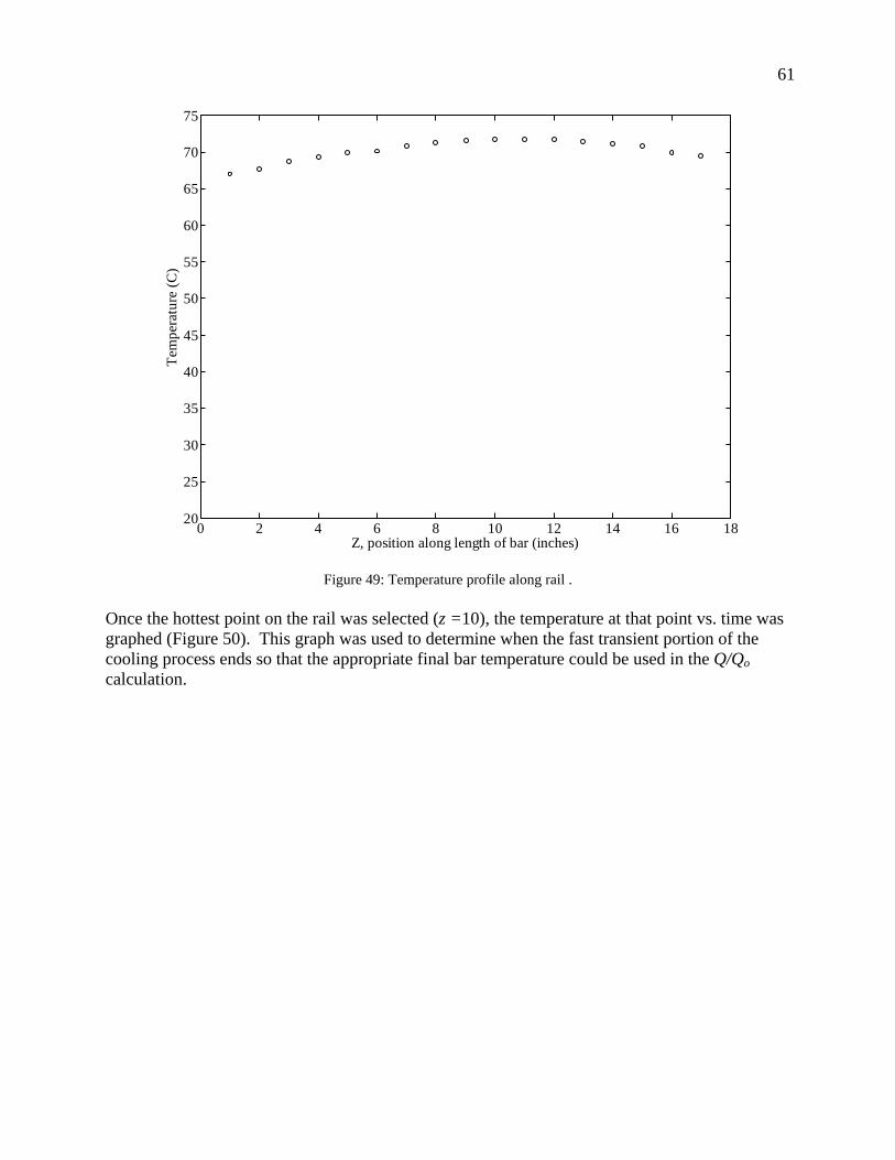
61
0 2 4 6 8 10 12 14 16 1820
25
30
35
40
45
50
55
60
65
70
75
Tem
pera
ture
(C)
Z, position along length of bar (inches)
Figure 49: Temperature profile along rail . Once the hottest point on the rail was selected (z =10), the temperature at that point vs. time was graphed (Figure 50). This graph was used to determine when the fast transient portion of the cooling process ends so that the appropriate final bar temperature could be used in the Q/Qo calculation.

62
0 10 20 30 40 50 6035
40
45
50
55
60
65
70
75
Time
Bar
tem
pera
ture
(C) a
t Z=1
1.0
in
Figure 50: Temperature at thermocouple 10 vs. time. The experimental Q/Qo ratio is calculated as shown in Eq. 50, except that the final rail temperature is determined from the graph above rather than from a weighted average of the modeled temperature profile. The results show that the bar is cooling down more quickly than predicted (Figure 51). One reason the Q/Qo ratio is lower than predicted is that the thermal entry region creates a non-uniform temperature distribution, which causes heat to flow in the z direction, while the assumption used in the model was for conduction in only one direction. Another reason that the Q/Qo ratio is lower than predicted could be that the transient heat transfer coefficient is higher while the thermal boundary layer is developing within the channel.

63
0 2 4 6 8 100
0.2
0.4
0.6
0.8
1
time (seconds)
Hea
t rat
io, Q
/ Q o
Predicted heat ratio
Actual heat ratio
Figure 51: Experimental and Theoretical Q/Qo ratios.
64
8.0 PROJECT CONCLUSIONS In order to develop a long range naval electromagnetic railgun that can be fired in a repetitive mode, the resistive heating of the rails in the railgun must be considered. To determine the optimal design for internal cooling channels in the rails, the compressive forces acting on the rails must also be taken into account. In fact, these forces ultimately limit the optimum cooling channel design. With the consideration of the resistive heating and compressive forces, an optimization routine was created to find the channel design for optimum heat transfer. This routine solves the heat equation for a fin with an elliptical boundary to find the channel design that has the lowest thermal resistance while meeting the defined structural constraints. The severity of the stresses acting on the rails also makes material selection an important element in the design. In the cooling channel optimization for the full size railgun, a beryllium copper alloy was chosen because it was the only alloy that met the basic requirements for the rail material based on its yield strength and thermal conductivity. In order to gain confidence in the optimization routine, the analytical expressions used to represent the stress concentration factors and heat equation were independently verified. First the uniaxial and biaxial stress concentration factors used in the optimization were confirmed using finite element analysis. For the channel geometries and stresses typical of the railgun application, the stress concentration factors found in the finite element analysis closely matched the analytical stress concentration factors. The heat transfer response predicted in the cooling channel design was verified through steady state experiments on copper rails with three different cooling channel designs. In this experiment, a heater was applied to one surface of the rail, and the rail temperature was measured along the length of the rail as water was pumped through the channels at various flow rates. The temperature data collected was used to calculate thermal resistance, and these values were compared to the values predicted in the optimization routine. The predicted values proved to be in reasonable agreement with the experimental results. Because the cooling of the rails in a railgun has a transient nature in the time between shots, the transient thermal response of the optimized channel design was also considered. An implicit finite difference method was used to predict the amount of heat removed (heat ratio) during a given time interval, and this quantity was then measured experimentally in order to verify the transient model. In the transient experiment, the rail was heated to a uniform temperature and cooling water was pumped through the channels for a range of time intervals. From the temperature data an experimental heat ratio was calculated for each time interval. The predicted and experimental results followed the same trend, but the experimental heat ratio was consistently lower than what was predicted. This can be attributed to the use of one dimensional analysis and a steady state heat transfer coefficient in the transient model. This project provides an optimization routine with analytical expressions for heat transfer and structural constraints that have been verified using independent measures. The confidence afforded by the methodology employed in this project indicates that this optimization routine is suitable for further analysis of a railgun cooling channel design.

65
AREAS FOR FURTHER STUDY A beryllium copper alloy was used in the full size railgun optimization out of necessity, but it is expensive and there are adverse health effects associated with prolonged exposure to beryllium compounds (Haz-Map 2004). Since there is little practicality in using such a material in actual railgun production, further research in material selection is imperative for railgun design to progress. Other potential alloys include chromium-copper and GlidCop® (Appendix 12). In this study cooling channels were optimized for steady state conditions, so the properties associated with transient heat transfer were not considered. For example, thermal diffusivity, the measure of how fast heat is transferred through a material, is not a factor in the current design. Since the physical railgun cooling problem has a transient nature, the optimization routine should be reevaluated to consider transient performance. Many simplifying assumptions were made in this design—the most significant being conduction in only one dimensional, steady state heating conditions, uniform compressive loads and the neglecting of any effects the cooling channels will have on the electrical current penetration and magnetic field distribution. The transient problem can be considered using methods similar to those used in this study, but further analysis in two or three dimensions introduces a level of complexity that necessitates a finite element analysis approach. These computational studies will need to consider the coupled thermal, mechanical and electromagnetic effects.

66
BIBLIOGRAPHY Bernardes, J.S., M.F. Stumborg, T.E. Jean, “Analysis of a Capacitor-Based Pulsed-Power
System for Driving Long-Range Electromagnetic Guns,” IEEE Transactions on Magnetics, Jan. 2003.
Clark, Vern. “Sea Power 21 Series—Part I: Projecting Decisive Joint Capabilities” U.S. Naval Institute Proceedings, October 2002.
Davis, J.R, ed. Copper and Copper Alloys. Materials Park, OH: ASM International, 2001. Ellis, R.L., J.C. Poynor, B.T. McGlasson, and A.N. Smith, “Influence of Bore and Rail
Geometry on an Electromagnetic Naval Railgun System,” To appear, IEEE Transactions on Magnetics, 2004.
Ellis, R.L. “Conversation concerning the railgun at Kircudbright, Scotland,” August 24, 2004. Fisher, T.S and K.E. Torrance, “Optimal Shapes of Fully Embedded Channels for Conjugate
Cooling,” IEEE Transactions on Advanced Packaging, Nov. 2001. Givens, Benjamin M. “USS South Carolina, BB-26 Battleship development”.
http://www.geocities.com/batdev/southcarolinabb-26class.html, December 24, 1999. Haz-Map, “Occupational Exposure to Hazardous Agents: Beryllium and Compounds”.
http://hazmap.nlm.nih.gov/cgi-bin/hazmap_generic?tbl=TblAgents&id=8, July 20, 2004. Incropera, F.P. and D.P. DeWitt, Fundamentals of Heat and Mass Transfer, Fifth Edition. New
York: Wiley, 2002. Jones, N. and D. Hozos, “A Study of the Stresses around Elliptical Holes in Flat Plates,” Journal
of Engineering for Industry, May 1971. McNab, I.R, S. Fish, and F. Stefani, “Parameters for an Electromagnetic Naval Railgun,” IEEE
Transactions on Magnetics, Jan. 2001. Mel Fisher Maritime Society, “Cannon Survey Ammunition”.
http://www.melfisher.org/cannonsurvey/ammunition.htm, 2001. Peterson, R.E., Stress Concentration Factors. New York: Wiley, 1953. Press, W.H., S.A. Teukolsky, W.T. Vetterling, B.P. Flannery, Numerical Recipes in C: The Art
of Scientific Computing, Second Edition. Cambridge: Cambridge University Press, 1992. Ramanujan, S. Ramanujan’s Notebooks: Part III. Edited by B.C. Berndt. New York: Springer-
Verlag, 1991. Smith, A.N., R.L. Ellis, J.S. Bernardes, and A.E. Zielinski, “Thermal Management and Resistive
Rail Heating of a Large-Scale Electromagnetic Launcher,” IEEE Transactions on Magnetics, Jan. 2005
Spotts, M.F. and T.E. Shoup, Design of Machine Elements. Upper Saddle River, New Jersey: Prentice Hall, 1998.
Young, W.C. and R.G. Budynas, Roark’s Formulas for Stress and Strain, Seventh edition. New York: McGraw, 2002.

67
Appendix 1: Optimization Code (Matlab®) Optimization.m %This is the primary code of the optimization. Line 13 contains the actual %function (fmincon) that does the minimization. fmincon is a function found in the %Matlab® Optimization Toolbox. A, B, lb and ub are constraints on the geometric %values, and p0 is the initital guess. After line 13, the rest of the code is written to output %values calculated with the final solution (x). A=[1 0 0; 0 1 0 ; 0 0 1]; B=[0.01 ; 0.012 ; 0.01]; p0=[0.005 ; 0.01 ; 0.005]; lb=[0.0001;0.0001;0.0001]; ub=[1;1;1]; options = optimset('MaxFunEvals', 500,'MaxIter', 500,'TolCon',1e-50,'TolFun',1e-50,'TolX',1e-50); [x,fval,exitflag,output]=fmincon(@rfin,p0,A,B,[],[],lb,ub,@newstress,options); Ncell=3 x mu=x(2)/x(1); ta=x(3)/x(1); Rtotal=fval/Ncell %inputs: FS=1; yield=1*310*1000000; uniaxial=110286000; %definitions lambda=x(1)/(x(1)+x(3)); allow=yield/FS; %axial constraint nominal=uniaxial*(x(1)+x(3))/x(3); c1= 1.000+0.000*sqrt(1/mu)+2.000*1/mu; c2=-0.351-0.021*sqrt(1/mu)-2.483*1/mu; c3= 3.621-5.183*sqrt(1/mu)+4.494*1/mu; c4=-2.270+5.204*sqrt(1/mu)-4.011*1/mu; Ku=c1+c2*lambda+c3*(lambda)^2+c4*(lambda)^3 uniaxialmax=Ku*nominal %biaxial constraint sigma1=47124900; sigma2=68571400; width=0.0254; effwidth=width-2*x(2); sigma1p=sigma1*(width/effwidth) sigma2p=sigma2*((x(1)+x(3))/x(3)) biaxialstressratio=sigma1p/sigma2p if sigma1p/sigma2p < 1/mu;

68
Kb=-sigma1p/sigma2p+1+2/mu biaxialmax=sigma2p*(1+2/mu)-sigma1p 'middle L' else Kb=(sigma1p/sigma2p)*(1+2*mu)-1 biaxialmax=(sigma1p*(1+2*mu)-sigma2p) 'positive SL' end %Reynolds number for solution: rho=997; mu=855e-6; Aellipse=pi*x(1)*x(2); P=pi*(3*(x(1)+x(2))-sqrt((3*x(1)+x(2))*(x(1)+3*x(2)))); Dh=4*Aellipse/P Um=feval(@Umm,x) Re=rho*Dh*Um/mu %heat transfer coefficient for solution: h=feval(@hxcoef,x) exitflag rfin.m %This function defines the fin resistance (the quantity being minimized), which involves solving the %boundary value problem or the energy equation for a variable area fin. %The function bvp4c is used to solve this equation (testg) with its boundary %conditions (testbcg). The definition of rfin is the last line of this %code (line 13). function x=rfin(g); k=388; solinit=bvpinit(linspace(-0.99*g(2),0.99*g(2),10),[1,0]); sol=bvp4c(@testg,@testbcg,solinit,[],g); y=linspace(-0.99*g(2),0.99*g(2)); T=deval(y,sol); x=1/(-k*(g(1)+g(3))*T(2)); %hold on %plot(y,T(2,:)) testg.m %This function contains the energy equation for a fin with elliptical %boundaries. It is defined in terms of y, T and g, where g is an array if %(a,b,t). The heat transder coefficient is also dependent on g, and it is %defined here as a function handle that calls the function hxcoef.m

69
function dTdy=testg(y,T,g); h=feval(@hxcoef,g); k=388; xstar=g(1)+g(3)-sqrt((1-y^2/g(2)^2)*g(1)^2); dTdy=[T(2);(-(g(1)/g(2))*y*T(2)/sqrt(g(2)^2-y^2)+(h/k)*T(1)*sqrt(1+(-y*(g(1)/g(2))/sqrt(g(2)^2-y^2))^2))/xstar]; testbcb.m %This function contains the boundary condidtions for the function in %testg.m function res=testbc(Ta,Tb,g) res=[Ta(1)-1;Tb(2)]; hxcoef.m %The heat transfer coefficient is a function of many variables, many of which are %affected by the geometry of the channel (g). The fluid properties are assumed to %be constant and taken at room temperature. The mean fluid velocity (Um) must be %determined by a separate function (Umm.m). function x=hxcoef(g); Um=feval(@Umm,g); rho=997; mu=0.0008905; Cp=4183; kf=0.5948; Aellipse=pi*g(1)*g(2); P=pi*(3*(g(1)+g(2))-sqrt((3*g(1)+g(2))*(g(1)+3*g(2)))); Dh=4*Aellipse/P; Re=rho*Dh*Um/mu; Pr=Cp*mu/kf; f=(0.79*log(Re)-1.64)^(-2); Nu=((f/8)*(Re-1000)*Pr)/(1+12.7*sqrt(f/8)*(Pr^(2/3)-1)); x=Nu*kf/Dh; pumpconstraint.m %The pump constraint in this case is ? Watts/meter. %pumppower=10/Ncell (per unit length) %pumppower=pressuredrop*Aellipse*Um (per unit length) %10/Ncell=pressuredrop*Aellipse*Um (per unit length) %in order to find the value of Um, the equation is manipulated to so that %the zero of the equation will be the value of Um: %x=pressuredrop*Aellipse*Um-?/Ncell

70
function x=pumpconstraint(Um,g); Ncell=3; rho=997; mu=855e-6; Aellipse=pi*g(1)*g(2); P=pi*(3*(g(1)+g(2))-sqrt((3*g(1)+g(2))*(g(1)+3*g(2)))); %Perimeter% Dh=4*Aellipse/P; Re=rho*Dh*Um/mu; f=(0.791*log(abs(Re))-1.64)^(-2); pressuredrop=f*rho*Um^2/(2*Dh); x=pressuredrop*Aellipse*Um-1.9184150576964/Ncell; Umm.m %This mean fluid velocity is determined by finding the zero of the pump %constraint equation (pumpconstraint.m) function x=Umm(g); x=bisect('pumpconstraint',0.01,30,g); bisect.m function root = bisect ( f, a, w, g) fa = feval ( f, a, g); fw = feval ( f, w, g); if ( sign ( fa ) == sign ( fw ) ) 'BISECT - Fatal error!' ' [A,w] is not a change-of-sign interval.' root = 0; return end format long while ( abs ( w - a ) > 0.000001 ) c = ( a + w ) / 2; fc = feval ( f, c, g ); [ a, c, w ; fa, fc, fw ]; if ( fc == 0 ) root = c; return elseif ( sign ( fc ) == sign ( fa ) )

71
a = c; fa = fc; elseif ( sign ( fc ) == sign ( fw ) ) w = c; fw = fc; end end root = 0.5 * ( a + w ); newstress.m %This file contains all of the structural constraints that are place on the %optimization. function [c,ceq]=newstress(g); %inputs: FS=1; yield=1*310*1000000; allow=yield/FS; Ncell=3; height=0.0508; cellwidth=height/Ncell; uniaxial=110286000; sigma1=47124900; sigma2=68571400; width=0.0254; effwidth=width-2*g(2); sigma1p=sigma1*(width/effwidth); sigma2p=sigma2*((g(1)+g(3))/g(3)); %definitions mu=g(2)/g(1); lambda=g(1)/(g(1)+g(3)); %axial constraint nominal=uniaxial*(g(1)+g(3))/g(3); c1= 1.000+0.000*sqrt(1/mu)+2.000*1/mu; c2=-0.351-0.021*sqrt(1/mu)-2.483*1/mu; c3= 3.621-5.183*sqrt(1/mu)+4.494*1/mu; c4=-2.270+5.204*sqrt(1/mu)-4.011*1/mu; Kc=c1+c2*lambda+c3*(lambda)^2+c4*(lambda)^3; %biaxial constraint if sigma1p/sigma2p < 1/mu; K=-sigma1p/sigma2p+1+2/mu; sigmamax=sigma2p*(1+2/mu)-sigma1p; 'middle line used';

72
else K=(sigma1p/sigma2p)*(1+2*mu)-1; sigmamax=(sigma1p*(1+2*mu)-sigma2p); 'positive slope line used'; end %minimum effective height constraint sigmaarea=uniaxial*height/(Ncell*2*g(3)); c=[Kc*nominal-allow;sigmamax-allow;0]; %mineffh-2*g(3)*Ncell %unit cell constraint ceq=[g(1)+g(3)-cellwidth/2;0;0];

Appendix 2: Full Size Railgun Optimization Results
73
Rai
l Mat
eria
l Pro
pert
ies:
Rai
l Cro
ss S
ectio
n Si
ze:
Com
pres
sive
For
ces:
Ber
ylliu
m C
oppe
r (U
NS
C17
600)
heig
ht=0
.135
mU
niax
ial s
tress
: 386
MP
aY
ield
Stre
ngth
: 825
MP
aw
idth
=0.0
61m
Bia
xial
stre
ss: 1
=280
Mpa
, 2=1
65 M
paTh
erm
al C
ondu
ctiv
ity: 2
15 W
/m-K
Flui
d C
onst
rain
t:P
ower
per
cha
nnel
=10
0/N
cell
No.
of U
nit C
ells
(N
cell)
1413
1211
109
a (m
)0.
0013
730.
0014
650.
0015
690.
0016
890.
0018
290.
0019
93b
(m)
0.00
3752
0.00
3960
0.00
4192
0.00
4452
0.00
4744
0.00
5076
t (m
)0.
0034
480.
0037
280.
0040
560.
0044
470.
0049
210.
0055
07
(b/a
)2.
733
2.70
42.
671
2.63
52.
594
2.54
7t/a
2.51
22.
545
2.58
52.
632
2.69
02.
763
R to
tal'
(K-m
/W)
5.85
1E-0
46.
005E
-04
6.17
9E-0
46.
377E
-04
6.60
5E-0
46.
872E
-04
Uni
axia
l K1.
529
1.53
41.
541
1.54
91.
558
1.56
9U
niax
ialm
ax (
Pa)
8.25
0E+0
88.
250E
+08
8.25
0E+0
88.
250E
+08
8.25
0E+0
88.
250E
+08
1'
(Pa)
1.88
1E+0
81.
896E
+08
1.91
3E+0
81.
932E
+08
1.95
4E+0
81.
979E
+08
sigm
a2' (
Pa)
3.91
5E+0
83.
900E
+08
3.88
3E+0
83.
864E
+08
3.84
1E+0
83.
813E
+08
sigm
a1'/s
igm
a2'
0.48
10.
486
0.49
30.
500
0.50
90.
519
Bia
xial
K2.
107
2.11
52.
124
2.13
52.
148
2.16
4B
iaxi
alm
ax (
Pa)
8.25
0E+0
88.
250E
+08
8.25
0E+0
88.
250E
+08
8.25
0E+0
88.
250E
+08
Bia
xial
cas
epo
sitiv
e sl
ope
line
posi
tive
slop
e lin
epo
sitiv
e sl
ope
line
posi
tive
slop
e lin
epo
sitiv
e sl
ope
line
posi
tive
slop
e lin
eD
h (m
)0.
0038
130.
0040
590.
0043
390.
0046
600.
0050
300.
0054
61U
m (m
/s)
5.11
45.
178
5.24
95.
329
5.42
15.
528
Re
2.27
4E+0
42.
451E
+04
2.65
6E+0
42.
896E
+04
3.18
0E+0
43.
520E
+04
h (W
/m^2
K)
2.39
1E+0
42.
397E
+04
2.40
5E+0
42.
415E
+04
2.42
6E+0
42.
441E
+04
exitf
lag
00
00
00
R c
ell'
(K-m
/W)
8.19
1E-0
30.
0078
0659
60.
0074
1442
70.
0070
1416
30.
0066
0460
90.
0061
8501
4
= (a
/(a+t
))0.
2847
7172
20.
2820
9032
70.
2789
7757
90.
2753
2236
90.
2709
7277
0.26
5715
976
2b/(0
.61)
0.01
2302
208
0.01
2984
486
0.01
3744
661
0.01
4596
208
0.01
5555
60.
0166
4299
6

Appendix 2: Full Size Railgun Optimization Results
74
Rai
l Mat
eria
l Pro
pert
ies:
Rai
l Cro
ss S
ectio
n Si
ze:
Com
pres
sive
For
ces:
Ber
ylliu
m C
oppe
r (U
NS
C17
600)
heig
ht=0
.135
mU
niax
ial s
tress
: 386
MP
aY
ield
Stre
ngth
: 825
MP
aw
idth
=0.0
61m
Bia
xial
stre
ss: 1
=280
Mpa
, 2=1
65 M
paTh
erm
al C
ondu
ctiv
ity: 2
15 W
/m-K
Flui
d C
onst
rain
t:P
ower
per
cha
nnel
=10
0/N
cell
No.
of U
nit C
ells
(N
cell)
87
65
4a
(m)
0.00
2187
0.00
2421
0.00
2707
0.00
306
0.00
3498
b (m
)0.
0054
540.
0058
880.
0063
870.
0069
60.
0076
20t (
m)
0.00
6250
0.00
7221
0.00
8543
0.01
0494
0.01
3377
Bet
a (b
/a)
2.49
42.
432
2.36
02.
275
2.17
8t/a
2.85
72.
982
3.15
63.
429
3.82
4R
tota
l (K
/W)
7.18
7E-0
47.
563E
-04
8.03
4E-0
48.
624E
-04
9.44
9E-0
4U
niax
ial K
1.58
31.
601
1.62
31.
654
1.69
4U
niax
ialm
ax (
Pa)
8.25
0E+0
88.
250E
+08
8.25
0E+0
882
4541
184.
530
8.25
0E+0
8si
gma1
' (P
a)2.
009E
+08
2.04
5E+0
82.
087E
+08
2.14
E+0
82.
200E
+08
sigm
a2' (
Pa)
3.78
0E+0
83.
739E
+08
3.68
7E+0
83.
62E
+08
3.53
2E+0
8si
gma1
'/sig
ma2
'0.
532
0.54
70.
566
0.59
1143
437
0.62
3B
iaxi
al K
2.18
32.
207
2.23
82.
2802
6652
32.
336
Bia
xial
max
(P
a)8.
250E
+08
8.25
0E+0
88.
250E
+08
8.25
E+0
88.
250E
+08
Bia
xial
cas
epo
sitiv
e sl
ope
line
posi
tive
slop
e lin
epo
sitiv
e sl
ope
line
posi
tive
slop
e lin
epo
sitiv
e sl
ope
line
Dh
(m)
0.00
5969
0.00
6574
0.00
7302
0.00
8188
901
0.00
9269
Um
(m/s
)5.
655
5.80
96.
002
6.25
4603
306
6.60
2R
e3.
936E
+04
4.45
3E+0
45.
111E
+04
5.97
E+0
47.
135E
+04
h (W
/m^2
K)
2.45
9E+0
42.
484E
+04
2.51
8E+0
42.
57E
+04
2.64
4E+0
4ex
itfla
g0
00
0R
cel
l5.
750E
-03
0.00
5294
240.
0048
2032
10.
0043
1210
30.
0037
7955
lam
bda
(a/(a
+t))
0.25
9245
622
0.25
1106
736
0.24
0599
791
0.22
5763
612
0.20
7290
138
2b/(0
.61)
0.01
7882
933
0.01
9304
767
0.02
0941
995
0.02
2819
672
0.02
4983
45

75 Appendix 3: Average Surface Temperature Calculations (Matlab®) Conclusion_calcs.m % final calculations for conclusion for i=1:1:50 time(i)=i*.5; end Heat=15000000; %Joules width=0.135; % meters length=10; % meters Area=length*width; q_flux=Heat./(time*Area); %Watts d=0.020; %meters k=215; %W/m-K R_doubleprime_conduction=d/k; R_cell_per_Length=0.000718707497568427; %for 8 channels in the full size rail R_doubleprime_fin=R_cell_per_Length*width; R__doubleprime_total=R_doubleprime_fin+R_doubleprime_conduction; T_inf=293; Delta_T=q_flux*R__doubleprime_total; %Kelvin or C T_surface=T_inf+Delta_T-273; %Celsius hold on plot(time,T_surface,'-black') plot(time(10),T_surface(10),'oblack') plot(time(20),T_surface(20),'oblack') axis([0 25 0 4500]) xlabel('time (seconds)') ylabel('Temperature (C)')
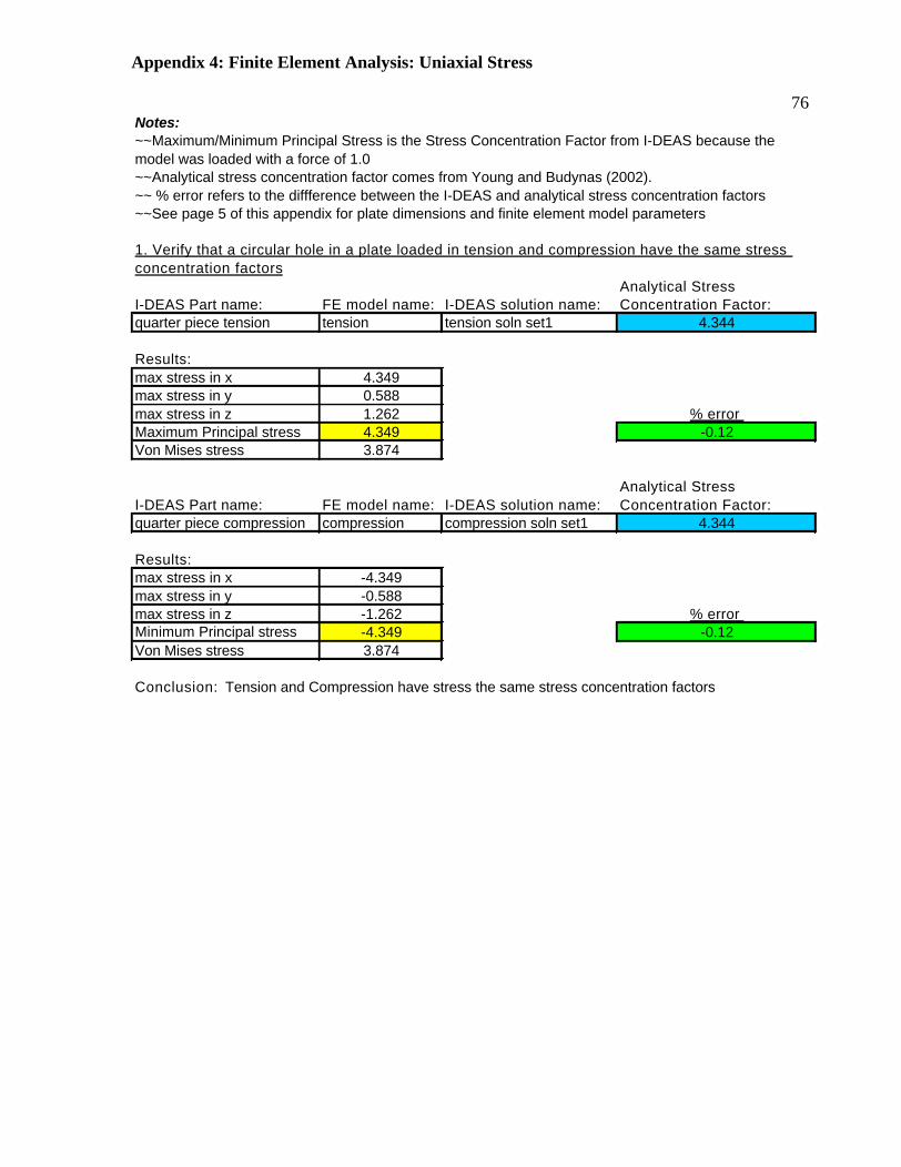
Appendix 4: Finite Element Analysis: Uniaxial Stress
76Notes:
~~Analytical stress concentration factor comes from Young and Budynas (2002).~~ % error refers to the diffference between the I-DEAS and analytical stress concentration factors~~See page 5 of this appendix for plate dimensions and finite element model parameters
Analytical Stress I-DEAS Part name: FE model name: I-DEAS solution name: Concentration Factor:quarter piece tension tension tension soln set1 4.344
Results: max stress in x 4.349max stress in y 0.588max stress in z 1.262 % error Maximum Principal stress 4.349 -0.12Von Mises stress 3.874
Analytical Stress I-DEAS Part name: FE model name: I-DEAS solution name: Concentration Factor:quarter piece compression compression compression soln set1 4.344
Results:max stress in x -4.349max stress in y -0.588max stress in z -1.262 % error Minimum Principal stress -4.349 -0.12Von Mises stress 3.874
Conclusion: Tension and Compression have stress the same stress concentration factors
~~Maximum/Minimum Principal Stress is the Stress Concentration Factor from I-DEAS because the model was loaded with a force of 1.0
1. Verify that a circular hole in a plate loaded in tension and compression have the same stress concentration factors
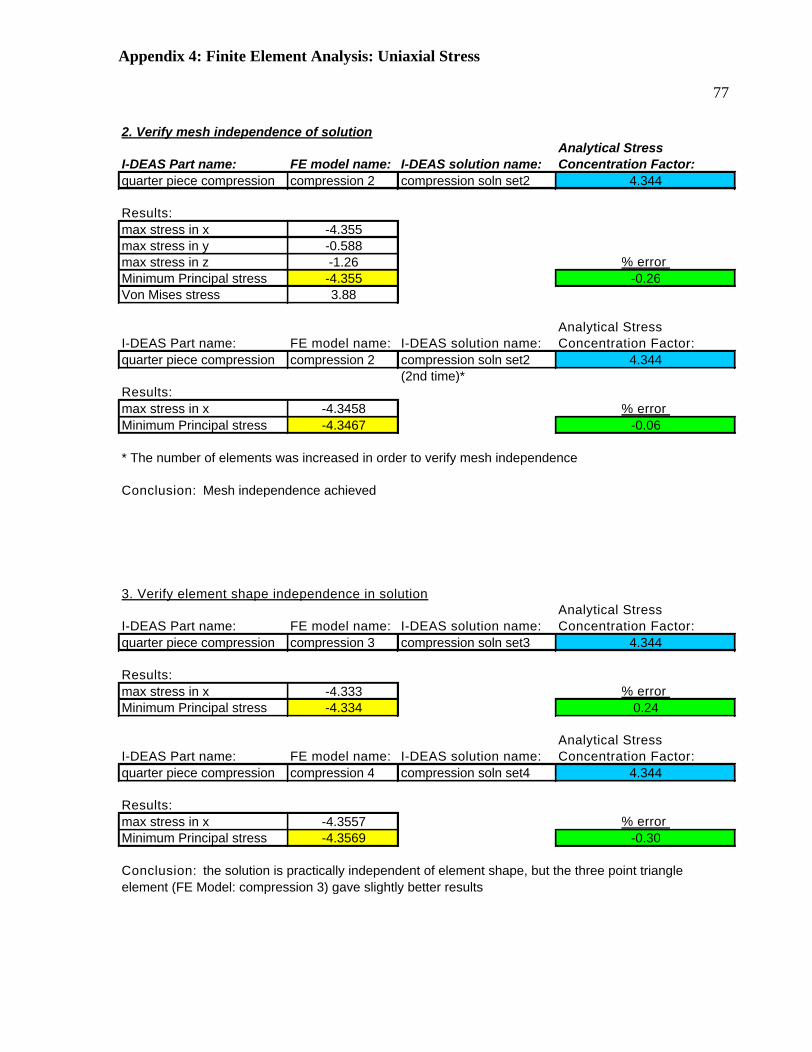
Appendix 4: Finite Element Analysis: Uniaxial Stress
77
2. Verify mesh independence of solutionAnalytical Stress
I-DEAS Part name: FE model name: I-DEAS solution name: Concentration Factor:quarter piece compression compression 2 compression soln set2 4.344
Results: max stress in x -4.355max stress in y -0.588max stress in z -1.26 % error Minimum Principal stress -4.355 -0.26Von Mises stress 3.88
Analytical Stress I-DEAS Part name: FE model name: I-DEAS solution name: Concentration Factor:quarter piece compression compression 2 compression soln set2 4.344
(2nd time)*Results: max stress in x -4.3458 % error Minimum Principal stress -4.3467 -0.06
* The number of elements was increased in order to verify mesh independence
Conclusion: Mesh independence achieved
3. Verify element shape independence in solutionAnalytical Stress
I-DEAS Part name: FE model name: I-DEAS solution name: Concentration Factor:quarter piece compression compression 3 compression soln set3 4.344
Results: max stress in x -4.333 % error Minimum Principal stress -4.334 0.24
Analytical Stress I-DEAS Part name: FE model name: I-DEAS solution name: Concentration Factor:quarter piece compression compression 4 compression soln set4 4.344
Results: max stress in x -4.3557 % error Minimum Principal stress -4.3569 -0.30
Conclusion: the solution is practically independent of element shape, but the three point triangle element (FE Model: compression 3) gave slightly better results

Appendix 4: Finite Element Analysis: Uniaxial Stress
78
Analytical Stress I-DEAS Part name: FE model name: I-DEAS solution name: Concentration Factor:quarter 2 compression 5 compression soln set5 4.344
Results: max stress in x -4.597 % error Minimum Principal stress -4.598 -5.84
Analytical Stress I-DEAS Part name: FE model name: I-DEAS solution name: Concentration Factor:quarter piece compression compression 3.5 compression soln set3.5 4.344
Results: max stress in x -4.3228 % error Minimum Principal stress -4.3228 0.49
4. Verify that the numerical solution matches the analytical solution for a range of plate sizes (hole is the same size and relative location)
Note: these cases were run to investigate the effect of overall plate length
Conclusion: the length of the plate in the direction of the force does affect the stress concentration factor, even though the equation from the literature does not account for this effect.

Appendix 4: Finite Element Analysis: Uniaxial Stress
79
Analytical Stress I-DEAS Part name: FE model name: I-DEAS solution name: Concentration Factor:quarter 3 compression 6 compression soln set 6 2.302
Results: max stress in x -2.260 % error Minimum Principal stress -2.261 1.77
Analytical Stress I-DEAS Part name: FE model name: I-DEAS solution name: Concentration Factor:quarter 4 compression 7 compression soln set7 1.99
Results: max stress in x -2.01 % error Minimum Principal stress -2.01 -1.01
Analytical Stress I-DEAS Part name: FE model name: I-DEAS solution name: Concentration Factor:quarter 5 compression 8 compression soln set8 6.565
Results: max stress in x -6.03 % error Minimum Principal stress -6.04 8.00
Analytical Stress I-DEAS Part name: FE model name: I-DEAS solution name: Concentration Factor:quarter 6 compression 9 compression soln set9 5.545
Results: max stress in x -5.27 % error Minimum Principal stress -5.29 4.60
Conclusion: For an ellipse the correlation is better when the aspect ratio (beta) is greater than one.However, for an aspect ratio less than 1, the analytical solution is conservative.
5. Verify that the numerical solution matches the analytical solution for an elliptical hole

Appendix 4: Finite Element Analysis: Uniaxial Stress
80
Part
Dim
ensi
ons
Part
ab
tb+
da+
tbe
ta=b
/aqu
arte
r pie
ce c
ompr
essi
on10
1010
5020
1qu
arte
r pie
ce te
nsio
n10
1010
5020
1qu
arte
r 210
1010
3020
1qu
arte
r 35
1015
5020
2qu
arte
r 45
1515
5020
3qu
arte
r 510
510
5020
0.5
quar
ter 6
105
2050
300.
5
Fini
te E
lem
ent M
odel
Par
amet
ers
FE m
odel
nam
e:sh
ape:
leng
th:
node
s on
qua
rter
circ
le:
elem
ent t
ype:
mes
h ty
pe:
tens
ion
6 pt
tria
ngle
525
plan
e st
rain
shel
lco
mpr
essi
on6
pt tr
iang
le5
25pl
ane
stra
insh
ell
com
pres
sion
26
pt tr
iang
le2
25pl
ane
stra
insh
ell
com
pres
sion
26
pt tr
iang
le2
50; 2
5 on
left,
35
on b
otto
mpl
ane
stra
insh
ell
com
pres
sion
33
pt tr
iang
le2
50; 2
5 on
left,
35
on b
otto
mpl
ane
stra
insh
ell
com
pres
sion
4qu
adril
ater
al2
50; 2
5 on
left,
35
on b
otto
mpl
ane
stra
insh
ell
com
pres
sion
53
pt tr
iang
le2
50; 2
5 on
left,
35
on b
otto
mpl
ane
stra
insh
ell
com
pres
sion
3.5
3 pt
tria
ngle
1.5
50; a
lot m
ore
node
spl
ane
stra
insh
ell
com
pres
sion
63
pt tr
iang
le2
50; 3
5 on
left,
75
on b
otto
mpl
ane
stra
insh
ell
com
pres
sion
73
pt tr
iang
le2
50; 3
5 on
left,
50
on b
otto
mpl
ane
stra
insh
ell
com
pres
sion
83
pt tr
iang
le2
50; 2
5, 7
5pl
ane
stra
insh
ell
Mes
h no
tes:
~~
plai
n st
rain
- st
rain
nor
mal
to th
e pl
ane
is z
ero,
this
repr
esen
ts a
sam
ple
that
is m
any
times
thic
ker t
han
the
elem
ent s
ize
~~sh
ell m
esh
- ele
men
t thi
ckne
ss is
not
con
side
red
in th
is m
esh

Appendix 5: Finite Element Analysis: Infinite Biaxial Stress
81
Test
cas
ePa
rt n
ame
FE m
odel
nam
eσ
1σ
2σ
1 / σ
21
/ βK
: Ana
lytic
alM
ax. P
rin. S
tres
sK
: I-D
EAS
% e
rror
1in
finite
bet
a 1
ratio
1 b
eta
11.
01.
01
12.
002.
032.
03-1
.52
infin
ite b
eta
1ra
tio 2
bet
a 1
2.0
1.0
21
5.00
5.03
2.52
49.7
3in
finite
bet
a 1
ratio
0.5
bet
a 1
0.5
1.0
0.5
12.
502.
532.
53-1
.24
infin
ite b
eta
1ra
tio 0
.1 b
eta
10.
11.
00.
11
2.90
2.92
2.92
-0.7
5in
finite
bet
a 1
ratio
-0.5
bet
a 1
0.5
-1.0
-0.5
12.
502.
462.
461.
66
infin
ite b
eta
2ra
tio 1
bet
a 2
1.0
1.0
10.
54.
033.
953.
952.
07
infin
ite b
eta
2ra
tio 2
bet
a 2
2.0
1.0
20.
54.
548.
804.
403.
18
infin
ite b
eta
2ra
tio 0
.5 b
eta
20.
51.
00.
50.
51.
541.
531.
530.
69
infin
ite b
eta
2ra
tio 0
.1 b
eta
20.
11.
00.
10.
51.
941.
921.
921.
010
infin
ite b
eta
2ra
tio -0
.5 b
eta
20.
5-1
.0-0
.50.
53.
553.
323.
326.
511
infin
ite b
eta
2ra
tio 0
.75
beta
20.
81.
00.
750.
52.
773.
363.
36-2
1.3
12in
finite
bet
a 3
ratio
1 b
eta
31.
01.
01
0.33
6.04
4.68
4.68
22.5
13in
finite
bet
a 3
ratio
2 b
eta
32.
01.
02
0.33
6.56
9.93
4.97
24.3
14in
finite
bet
a 3
ratio
0.5
bet
a 3
0.5
1.0
0.5
0.33
2.51
2.07
2.07
17.5
15in
finite
bet
a 3
ratio
0.1
bet
a 3
0.1
1.0
0.1
0.33
1.62
1.57
1.57
3.1
16in
finite
bet
a 3
ratio
-0.5
bet
a 2
0.5
-1.0
-0.5
0.33
4.57
3.21
3.21
29.8
17in
finite
bet
a 3
ratio
3 b
eta
33.
01.
03
0.33
6.73
15.2
05.
0724
.718
infin
ite b
eta
3ra
tio -1
bet
a 3
1.0
-1.0
-10.
338.
105.
845.
8427
.919
infin
ite b
eta
3ra
tio -2
bet
a 3
2.0
-1.0
-20.
337.
5911
.10
5.55
26.9
Par
t dim
ensi
ons
Par
ta
bt
b+d
a+t
beta
=b/a
infin
ite b
eta
12
219
820
020
01
infin
ite b
eta
22
419
820
020
02
infin
ite b
eta
32
619
820
020
03
Not
es:
~~ σ
1 is
act
ing
in th
e y
dire
ctio
n (u
p an
d do
wn)
, σ 2
act
s in
the
x di
rect
ion
~~ a
is in
the
y di
rect
ion,
b is
in th
e x
dire
ctio
n
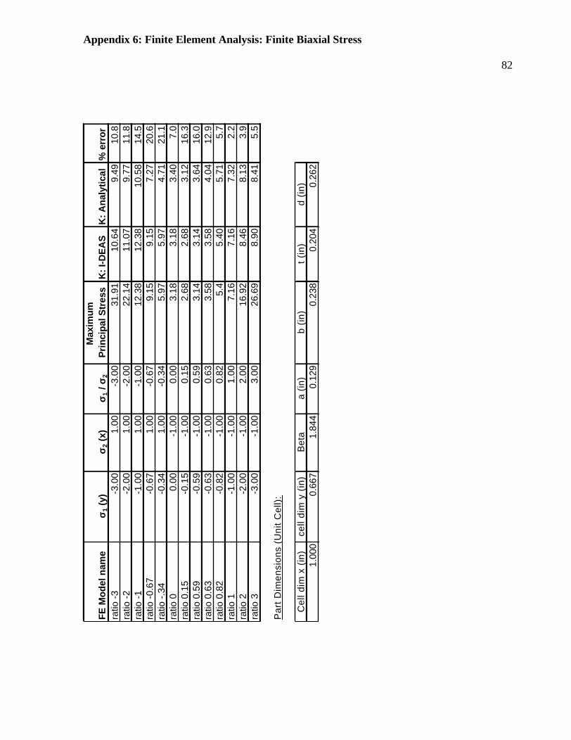
Appendix 6: Finite Element Analysis: Finite Biaxial Stress
82
Max
imum
FE
Mod
el n
ame
σ 1 (y
)σ 2
(x)
σ 1 /
σ 2
Prin
cipa
l Str
ess
K: I
-DEA
SK
: Ana
lytic
al%
err
orra
tio -3
-3.0
01.
00-3
.00
31.9
110
.64
9.49
10.8
ratio
-2-2
.00
1.00
-2.0
022
.14
11.0
79.
7711
.8ra
tio -1
-1.0
01.
00-1
.00
12.3
812
.38
10.5
814
.5ra
tio -0
.67
-0.6
71.
00-0
.67
9.15
9.15
7.27
20.6
ratio
-.34
-0.3
41.
00-0
.34
5.97
5.97
4.71
21.1
ratio
00.
00-1
.00
0.00
3.18
3.18
3.40
7.0
ratio
0.1
5-0
.15
-1.0
00.
152.
682.
683.
1216
.3ra
tio 0
.59
-0.5
9-1
.00
0.59
3.14
3.14
3.64
16.0
ratio
0.6
3-0
.63
-1.0
00.
633.
583.
584.
0412
.9ra
tio 0
.82
-0.8
2-1
.00
0.82
5.4
5.40
5.71
5.7
ratio
1-1
.00
-1.0
01.
007.
167.
167.
322.
2ra
tio 2
-2.0
0-1
.00
2.00
16.9
28.
468.
133.
9ra
tio 3
-3.0
0-1
.00
3.00
26.6
98.
908.
415.
5
Par
t Dim
ensi
ons
(Uni
t Cel
l):
Cel
l dim
x (
in)
cell
dim
y (
in)
Bet
aa
(in)
b (in
)t (
in)
d (in
)1.
000
0.66
71.
844
0.12
90.
238
0.20
40.
262

The values presented are typical and not intended for specification purposes. This information is provided without warranty, representation, inducement or license of any kind, including, but not limited to implied warranties of merchantability and fitness for a particular use or purpose, except that it is accurate to the best of American Micro Industries’ knowledge or obtained from sources believed by American Micro Industries to be accurate, and American Micro Industries does not assume any legal responsibility for the use or reliance upon same, as well as any typographical errors. Users of our product(s) are encouraged to conduct their own tests for suitability and conformance.
Rev. 5/17/04
AMERICAN MICRO Industries, Inc. 440 C Ramsey Avenue, Chambersburg, PA 17201
Tel: (800) 558-2058 Fax: (717) 261-9161 e-mail: [email protected]
Material Specifications for G10/FR4 Properties NEMA grade reinforcement~resin binder, glass-epoxies Tensile Strength Lengthwise, PSI 40,000 Crosswise, PSI 35,000 Compressive Strength Flatwise, PSI 60,000 Edgewise, PSI 35,000 Flexural Strength Lengthwise, PSI 55,000 Edgewise, PSI 45,000 Modulus of Elasticity in Flex Lengthwise, PSI x 10 6 2.7 Crosswise, PSI x 10 6 2.2 Shear Strength, PSI 19,000 IZOD Impact Flatwise, ft lb per inch of notch 7 Edgewise, ft lb per inch of notch 5.5 Rockwell Hardness M Scale 110 Specific Gravity 1.82 Coefficient of Thermal Expansion cm/cm deg C x 10 -5 .9 Water Absorption 0.62” thick, % per 24 hrs 0.25 0.125” thick, % per 24 hrs 0.15 0.500” tick, % per 24 hrs 0.10 Dielectric Strength, volt/mil 0.062” thick (perpendicular to laminations; short) 500 0.125” thick (perpendicular to laminations; short) 400 Dissipation Factor condition A, 1 megacycle 0.025 Dielectric Constant condition A, 1 megacycle 5.2 Insulation Resistance Condition: 96 hrs at 90% relative humidity (in mega ohms) 200,000 Flame Resistance Underwriter Labs, Classification 94V-0 Bond Strength in lbs 2,000 Max Continuous Operating Temperature Approximate degrees oF 285

Appendix 8: Thermocouple Calibration
84
icebath2.m%This file contains the data from the thermocouple calibration, and running this produces the %matrices 'ice' and 'boil' which are used in the steady state calculations. Consequently, this file %must be run before the files containing the steady state %calculations must be run
x=[0;1;2;3;4;5;6;7;8;9;10;11;12;13;14;15;16;17;18];ice=[0;0.21759519480519487; 0.14695818181818177; 0.2727576623376624;
0.12027805194805201; 0.2511764935064935; 0.09331064935064941;0.035655194805194815; 0.3833594805194806; 0.04666545454545456;0.1989222077922078; 0.02924597402597404; 0.10564740259740257;0.33213311688311703; 0.24440649350649354; 0.45613961038961043;
0.3643548051948051; 0.42522597402597395;0];
figure(2)plot(x,ice,'oblue')title('Thermocouple reading in an icebath 2 vs. thermocouple number') %xlabel ('thermocouple number')ylabel ('Temperature (C)') %
boil=[100;100.0648827777778; 100.06630111111112; 100.30158266666662;100.2308548888889; 100.19585133333337; 100.04096233333333;100.00681766666662; 100.38428022222222; 100.06214277777781;100.20797055555555; 100.13512822222219; 100.24105055555557;100.2351358888889; 100.36998788888886; 100.45128022222222;100.32367366666666; 100.44321611111106;100];
figure(3)plot(x,boil,'ored')title('Thermocouple reading in an boiling distilled water vs. thermocouple number') %xlabel ('thermocouple number')ylabel ('Temperature (C)') %
difference=boil-ice
figure(4)plot(x,difference,'omagenta')title('Temperature difference (boil-ice) vs. thermocouple number') %xlabel ('thermocouple number')ylabel ('Temperature (C)') %
%Note: points 0 and 18 were not actually measured, they are place holders

85 Appendix 9: Steady State Data (Matlab®) This is a sample code used to manipulate the steady state data. The subsequent codes for various flow rates and channel geometries are identical except for the rail temperatures (LPM2) and water temperatures (waterIN2LPM and waterOUT2LPM). iLPM2data.m %in order to get the legend to work correctly, all the LPM2data, etc files %need to be run in order by increasing flow rate. hold on axis([0 18 0 12]) title('Temperature Difference vs. Length Along Bar') % xlabel ('X (in)') ylabel ('Temperature Difference (C)') % x=[0;1;2;3;4;5;6;7;8;9;10;11;12;13;14;15;16;17;18]; LPM2=[0;23.99;25.527;27.085;27.89;28.886;29.219;29.409;30.168;29.737;30.218;29.87;30.176;30.582;0;30.47;30.565;29.774;0;]; waterIN2LPM=[19.64015111;19.53934189;19.50703789]; waterOUT2LPM=[22.02495811;22.02905856;22.01340467]; IN=sum(waterIN2LPM)/3; OUT=sum(waterOUT2LPM)/3; deltay=(OUT-IN); deltax=18; m=deltay/deltax; y=m*x; plot(x,y,'black') theta2=(LPM2-ice)*100./(boil-ice)-IN; plot(x,theta2,'oblack') length=18*0.0254; %meters qPerLength=(1000/6)/length; %Watts/meter% there are 6 half-unit cells in the bar for i=1:19 deltaT(i)=theta2(i)-y(i); uaPerLength(i)=qPerLength/deltaT(i); rfinPerLength(i)=deltaT(i)/qPerLength; end UAPerLength=uaPerLength' R_finPerLength=rfinPerLength' %'Note: units for UA are W/m-K, units for R_fin are K-m/W'

86 %'the negative values do not correlate with data, they are only being used as placeholders.' R_sum=R_finPerLength(8)+R_finPerLength(9)+R_finPerLength(10)+R_finPerLength(11)+R_finPerLength(12)+R_finPerLength(13)+R_finPerLength(14); R_fin_PerLength_AVERAGE=R_sum/7
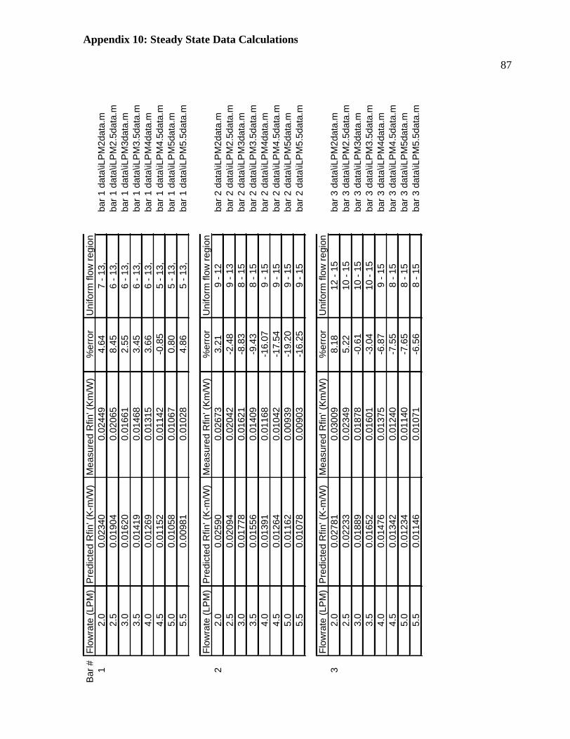
Appendix 10: Steady State Data Calculations
87
Bar #
Fl
owra
te (L
PM)
Pre
dict
ed R
fin' (
K-m
/W)
Mea
sure
d R
fin' (
Km/W
)%
erro
rU
nifo
rm fl
ow re
gion
12.
00.
0234
00.
0244
94.
647
- 13,
bar 1
dat
a\iL
PM2d
ata.
m2.
50.
0190
40.
0206
58.
456
- 13,
bar 1
dat
a\iL
PM2.
5dat
a.m
3.0
0.01
620
0.01
661
2.55
6 - 1
3,ba
r 1 d
ata\
iLPM
3dat
a.m
3.5
0.01
419
0.01
468
3.45
6 - 1
3,ba
r 1 d
ata\
iLPM
3.5d
ata.
m4.
00.
0126
90.
0131
53.
666
- 13,
bar 1
dat
a\iL
PM4d
ata.
m4.
50.
0115
20.
0114
2-0
.85
5 - 1
3,ba
r 1 d
ata\
iLPM
4.5d
ata.
m5.
00.
0105
80.
0106
70.
805
- 13,
bar 1
dat
a\iL
PM5d
ata.
m5.
50.
0098
10.
0102
84.
865
- 13,
bar 1
dat
a\iL
PM5.
5dat
a.m
Flow
rate
(LPM
)P
redi
cted
Rfin
' (K
-m/W
)M
easu
red
Rfin
' (Km
/W)
%er
ror
Uni
form
flow
regi
on2
2.0
0.02
590
0.02
673
3.21
9 - 1
2ba
r 2 d
ata\
iLPM
2dat
a.m
2.5
0.02
094
0.02
042
-2.4
89
- 13
bar 2
dat
a\iL
PM2.
5dat
a.m
3.0
0.01
778
0.01
621
-8.8
38
- 15
bar 2
dat
a\iL
PM3d
ata.
m3.
50.
0155
60.
0140
9-9
.43
8 - 1
5ba
r 2 d
ata\
iLPM
3.5d
ata.
m4.
00.
0139
10.
0116
8-1
6.07
9 - 1
5ba
r 2 d
ata\
iLPM
4dat
a.m
4.5
0.01
264
0.01
042
-17.
549
- 15
bar 2
dat
a\iL
PM4.
5dat
a.m
5.0
0.01
162
0.00
939
-19.
209
- 15
bar 2
dat
a\iL
PM5d
ata.
m5.
50.
0107
80.
0090
3-1
6.25
9 - 1
5ba
r 2 d
ata\
iLPM
5.5d
ata.
m
Flow
rate
(LPM
)P
redi
cted
Rfin
' (K
-m/W
)M
easu
red
Rfin
' (Km
/W)
%er
ror
Uni
form
flow
regi
on3
2.0
0.02
781
0.03
009
8.18
12 -
15ba
r 3 d
ata\
iLPM
2dat
a.m
2.5
0.02
233
0.02
349
5.22
10 -
15ba
r 3 d
ata\
iLPM
2.5d
ata.
m3.
00.
0188
90.
0187
8-0
.61
10 -
15ba
r 3 d
ata\
iLPM
3dat
a.m
3.5
0.01
652
0.01
601
-3.0
410
- 15
bar 3
dat
a\iL
PM3.
5dat
a.m
4.0
0.01
476
0.01
375
-6.8
79
- 15
bar 3
dat
a\iL
PM4d
ata.
m4.
50.
0134
20.
0124
0-7
.55
8 - 1
5ba
r 3 d
ata\
iLPM
4.5d
ata.
m5.
00.
0123
40.
0114
0-7
.65
8 - 1
5ba
r 3 d
ata\
iLPM
5dat
a.m
5.5
0.01
146
0.01
071
-6.5
68
- 15
bar 3
dat
a\iL
PM5.
5dat
a.m

Appendix 10: Steady State Data Calculations
88
Bar #
b
(m)
Flow
rate
(LPM
)Fl
uid
velo
city
- U
m (m
/s)
Pow
er (
W/m
)P
redi
cted
Rfin
' (K
-m/W
)a
(m)
0.00
3281
10.
0045
20.
7186
6838
90.
1223
0738
80.
0234
0t (
m)
0.00
5186
2.5
0.89
8335
487
0.22
3684
005
0.01
904
31.
0780
0258
40.
3668
8548
90.
0162
03.
51.
2576
6968
10.
5580
4901
40.
0141
94
1.43
7336
779
0.80
3100
179
0.01
269
4.5
1.61
7003
876
1.10
7793
238
0.01
152
51.
7966
7097
41.
4777
3642
60.
0105
85.
51.
9763
3807
11.
9184
1505
80.
0098
1
20.
0061
20.
5345
1796
20.
0651
0010
10.
0259
02.
50.
6681
4745
30.
1188
2608
0.02
094
30.
8017
7694
40.
1946
0282
70.
0177
83.
50.
9354
0643
40.
2956
3824
20.
0155
64
1.06
9035
925
0.42
5026
985
0.01
391
4.5
1.20
2665
415
0.58
5773
577
0.01
264
51.
3362
9490
60.
7808
0282
10.
0116
25.
51.
4699
2439
71.
0129
7694
60.
0107
8
30.
0076
20.
4255
2733
60.
0410
9896
60.
0278
12.
50.
5319
0917
0.07
4881
735
0.02
233
30.
6382
9100
40.
1224
6532
50.
0188
93.
50.
7446
7283
80.
1858
4033
10.
0165
24
0.85
1054
672
0.26
6928
066
0.01
476
4.5
0.95
7436
506
0.36
7591
733
0.01
342
51.
0638
1834
0.48
9644
624
0.01
234
5.5
1.17
0200
174
0.63
4860
543
0.01
146
How
to g
et P
redi
cted
Rfin
':
~Run
the
func
tion
flow
1.m
, flo
w2.
m, f
low
3.m
. Th
e an
swer
giv
en b
y M
atla
b is
the
pum
p po
wer
per
uni
t len
gth.
~P
ut th
is c
alcu
late
d pu
mp
pow
er p
er u
nit l
engt
h in
to th
e fu
nctio
n pu
mpc
onst
rain
t.m in
the
fold
er S
tead
y st
ate
calc
ulat
ions
~Run
Rfin
(g).m
, to
do th
is, y
ou a
lso
need
test
g.m
, tes
tbcg
.m, h
xcoe
f.m, U
mm
.m, p
umpc
onst
rain
t.m a
nd b
isse
ctbb
.m~D
efin
e g=
[a;b
;t]; i
n m
eter
s
~Fin
d flu
id v
eloc
ity b
y in
putin
g th
e flo
wra
te in
LPM
into
the
func
tion
for e
ach
rail;
flow
cons
train
t1.m
, flo
wco
nstra
int2
.m, f
low
cons
train
t3.m
. Th
ese
files
are
in th
e fo
lder
s fo
r the
resp
ectiv
e ch
anne
l geo
met
ries
(bar
1 d
ata,
etc
.)

89
Appendix 11: Transient Model middle_temp.m %Inputs from experiment: % time h -- based on flow rate and channel geometry clear all for m=1:1:10 Time=[1;2;3;4;5;6;7;8;9;10];% The time is entered this way instead of just through a for loop so I can put in times that are not nice clean numbers like here time(m)=Time(m); a=0.00328086088597; % from optimization with experimental parameters b=0.00605032567597; % from optimization with experimental parameters t=0.0051858057807; % from optimization with experimental parameters cell_dim_y=a+t; cell_dim_x=1*0.0254; %1 inch (length of experimental rail cross section) d=0.5*(cell_dim_x-2*b); % distance between edge of rail and channel (x direction) rho_bar=8936; %kg/m, from EES, T=T_inf Cp_bar=383; %J/kg-K, from EES, T=T_inf k_bar=388; %W/m-K, from EES, T=T_inf h_water=7.249582579872966e+003; %%%%% flow rate affects h---from to hxcoeff.m b_node_quantity=100; dx_b=2*b/(b_node_quantity-1); dt=0.0005; % time = 10; %%% use this instead of initial for loop (which creates a % matrix of time values) when you want a solution for only one time % interval number_of_timesteps=round(time(m)/dt); T_inf=293; %%%%Kelvin Fo_b=(k_bar*dt)/(dx_b^2*rho_bar*Cp_bar); % Fourier number d_node_quantity=floor(d/dx_b); %floor function rounds down to the nearest integer extra_node_length=d-d_node_quantity*dx_b; %this accounts for the extra length that will be added to the elements %on each end of the unit cell. This extra length is a product of %placing a node at the endge of the ellipse and maintaining a uniform %dx across the unit cell total_node_quantity=2*d_node_quantity+b_node_quantity; dx=dx_b; for i=1:1:total_node_quantity

90
xj(1) = 0; xj(i) = (dx*(i-1))+extra_node_length; xj(total_node_quantity) = (dx*(i-1))+2*extra_node_length; %xj and yj values are midway between nodes, to the right of the node end for i=1:1:total_node_quantity-1 %this for loop defines the x and y coordinates of the ellipse across %the whole unit cell if i <= d_node_quantity x(i)=0; y_ellipse(i) =0; elseif i >= (d_node_quantity+b_node_quantity) x(i)=0; y_ellipse(i) = 0; else x(i) = (xj(i)+xj(i+1))/2 - (b+d) ; y_ellipse(i) = sqrt(a^2*(1-x(i)^2/b^2)); %to check, plot(xj,y_ellipse,'o') axis([0 0.06 -0.06 0.06]) end yj = cell_dim_y - y_ellipse; end yj(total_node_quantity) = cell_dim_y; for i=1:1:total_node_quantity % this for loop defines the length of the channel boundary for each % element if i < d_node_quantity LinS(i)=0; elseif i == d_node_quantity+1 LinS(i) = sqrt ((x(i)--b)^2 + (y_ellipse(i)-0)^2); elseif i == d_node_quantity+b_node_quantity LinS(i) = sqrt ((b-x(i-1))^2 + (y_ellipse(i-1)-0)^2); elseif i > d_node_quantity+b_node_quantity LinS(i)=0; else

91
LinS(i) = sqrt ((x(i)-x(i-1))^2 + (y_ellipse(i)-y_ellipse(i-1))^2); %note: for verification, we checked that sum(LinS)=Perimeter of the %ellipse/2 end end yf(1) = cell_dim_y; yf(total_node_quantity) = cell_dim_y; for i=2:1:total_node_quantity-1; %this for loop defines the values of yf, the average height of an element yf(i)=(yj(i)+yj(i-1))/2; end yf(d_node_quantity+1) = 3/4*yj(d_node_quantity) + 1/4*yj(d_node_quantity+1); yf(d_node_quantity+b_node_quantity) = 1/4*yj(d_node_quantity+b_node_quantity-1) + 3/4 * yj(d_node_quantity+b_node_quantity); %these yf values are for the elements whose node falls at tne boundary of %the channel for i=1:1:total_node_quantity T(i)=273+300; %%%% This is the intial temperature of the unit cell end T_initial=T(i); for n=1:1:number_of_timesteps; %for each time step, the matrix will be generated and the %temperatures across the unit cell will be solved for for i=1:1:total_node_quantity; %this for loop defines column vectors of the coefficients a, b, c %and d which are terms in the heat equation if i == 1 a(i) = 0; else a(i) = -Fo_b*yj(i-1)/((yj(i)+yj(i-1))/2); % a(i) represents the energy coming from the left % hand side end b(i) = 1 + 2*Fo_b + h_water*LinS(i)*dt/(rho_bar*Cp_bar*dx*(yf(i))); % b(i) represents the energy coming from the node itself if i == total_node_quantity c(i) = 0; elseif i==1 c(1) = -Fo_b*yj(1)/yf(1);

92
else c(i) = -Fo_b*yj(i)/((yj(i)+yj(i-1))/2); % c(i) represents the energy coming from the right hand side end d(i) = T(i) + h_water*LinS(i)*dt*T_inf/(rho_bar*Cp_bar*dx*(yf(i))); % d(i) represents the energy at timestep n (as opposed to the % other column vectors which represent the energy at timestep % n+1) end a(total_node_quantity) = -Fo_b*yj(total_node_quantity-1)/yf(total_node_quantity); b(total_node_quantity) = 1 + Fo_b*(yj(total_node_quantity-1)/yf(total_node_quantity)) + h_water*LinS(total_node_quantity)*dt/(rho_bar*Cp_bar*dx*yf(total_node_quantity)); %this changes the right (back) edge node equation, we say that the %right edge is insulated, c(1) = -Fo_b*yj(1)/yf(1); b(1) = 1 + Fo_b*(yj(1)/yf(1)) + h_water*LinS(1)*dt/(rho_bar*Cp_bar*dx*yf(1)); %this changes the left (front) edge node equation, we say that the left %edge is insulated, T = Trimatrix(total_node_quantity,a,b,c,d); %Trimatrix is a sparse matrix solver T'; for i=1:1:total_node_quantity T_final=T; Syf=sum(yf); yfT(i)=yf(i)*T(i); SyfT=sum(yfT); T_final_average=SyfT/Syf; %This is a final temperature computed as a weighted average based %on the volume (which reduced to yf) of each node end if n==number_of_timesteps Q_ratio(m)=(T_initial-T_final_average)/(T_initial-T_inf); % This calculates the dimensionless heat ratio, Q/Qo, the ratio of % the heat removed to the total amount of heat that could be removed end hold all k=1:1:total_node_quantity; figure(m)
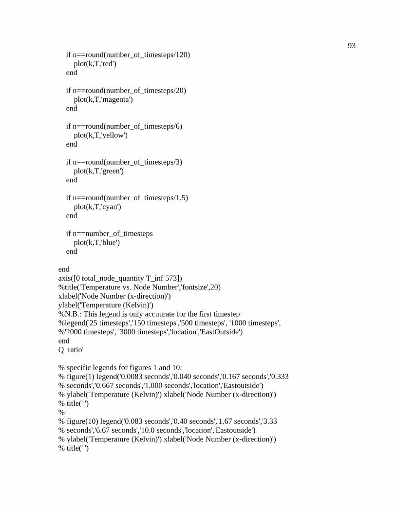
93
if n==round(number_of_timesteps/120) plot(k,T,'red') end if n==round(number_of_timesteps/20) plot(k,T,'magenta') end if n==round(number_of_timesteps/6) plot(k,T,'yellow') end if n==round(number_of_timesteps/3) plot(k,T,'green') end if n==round(number_of_timesteps/1.5) plot(k,T,'cyan') end if n==number_of_timesteps plot(k,T,'blue') end end axis([0 total_node_quantity T_inf 573]) %title('Temperature vs. Node Number','fontsize',20) xlabel('Node Number (x-direction)') ylabel('Temperature (Kelvin)') %N.B.: This legend is only accuurate for the first timestep %legend('25 timesteps','150 timesteps','500 timesteps', '1000 timesteps', %'2000 timesteps', '3000 timesteps','location','EastOutside') end Q_ratio' % specific legends for figures 1 and 10: % figure(1) legend('0.0083 seconds','0.040 seconds','0.167 seconds','0.333 % seconds','0.667 seconds','1.000 seconds','location','Eastoutside') % ylabel('Temperature (Kelvin)') xlabel('Node Number (x-direction)') % title(' ') % % figure(10) legend('0.083 seconds','0.40 seconds','1.67 seconds','3.33 % seconds','6.67 seconds','10.0 seconds','location','Eastoutside') % ylabel('Temperature (Kelvin)') xlabel('Node Number (x-direction)') % title(' ')

94
Trimatrix.m function T = Trimatrix(n,A,B,C,RHS) E(n) = 0; F(n) = 0; T(n) = 0; for i=1:1:n E(i + 1) = -(1 / ((B(i) + A(i) * E(i)))) * C(i); F(i + 1) = (1 / ((B(i) + A(i) * E(i)))) * (RHS(i) - A(i) * F(i)); end %--- Solution for the outer boundary -------------------------------- T(n) = F(n + 1); %--- Solution of the remaining by back substitution ----------------- for i = (n-1):-1:1 T(i) = E(i + 1) * T(i + 1) + F(i + 1); end
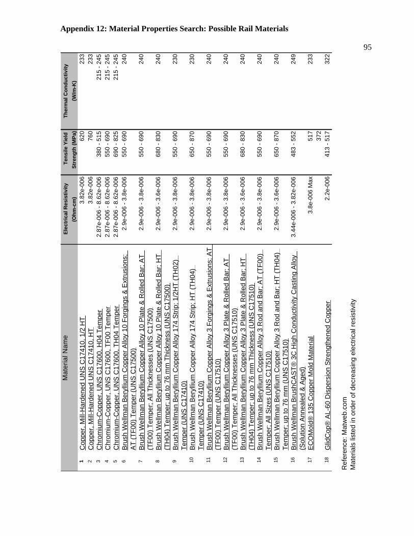
Appendix 12: Material Properties Search: Possible Rail Materials
95
Ele
ctric
al R
esis
tivity
T
ensi
le Y
ield
Th
erm
al C
ondu
ctiv
ity(O
hm-c
m)
Stre
ngth
(MPa
)(W
/m-K
)1
Cop
per,
Mill-
Har
dene
d U
NS
C17
410,
1/2
HT
3.8
2e-0
06 6
20 2
332
Cop
per,
Mill-
Har
dene
d U
NS
C17
410,
HT
3.8
2e-0
06 7
60 2
333
Chr
omiu
m-C
oppe
r, U
NS
C17
600,
H04
Tem
per
2.8
7e-0
06 -
8.62
e-00
6 3
80 -
515
215
- 24
54
Chr
omiu
m-C
oppe
r, U
NS
C17
600,
TF0
0 Te
mpe
r 2
.87e
-006
- 8.
62e-
006
550
- 69
0 2
15 -
245
5C
hrom
ium
-Cop
per,
UN
S C
1760
0, T
H04
Tem
per
2.8
7e-0
06 -
8.62
e-00
6 6
90 -
825
215
- 24
56
Brus
h W
ellm
an B
eryl
lium
Cop
per A
lloy
10 F
orgi
ngs
& Ex
trusi
ons;
AT
(TF0
0) T
empe
r (U
NS
C17
500)
2.9
e-00
6 - 3
.8e-
006
550
- 69
0 2
40
7Br
ush
Wel
lman
Ber
ylliu
m C
oppe
r Allo
y 10
Pla
te &
Rol
led
Bar;
AT
(TF0
0) T
empe
r; Al
l Thi
ckne
sses
(UN
S C
1750
0) 2
.9e-
006
- 3.8
e-00
6 5
50 -
690
240
8Br
ush
Wel
lman
Ber
ylliu
m C
oppe
r Allo
y 10
Pla
te &
Rol
led
Bar;
HT
(TH
04) T
empe
r; up
to 7
6 m
m T
hick
ness
(UN
S C
1750
0) 2
.9e-
006
- 3.6
e-00
6 6
80 -
830
240
9Br
ush
Wel
lman
Ber
ylliu
m C
oppe
r Allo
y 17
4 St
rip; 1
/2H
T (T
H02
) Te
mpe
r (U
NS
C17
410)
2.9
e-00
6 - 3
.8e-
006
550
- 69
0 2
30
10Br
ush
Wel
lman
Ber
ylliu
m C
oppe
r Allo
y 17
4 St
rip; H
T (T
H04
) Te
mpe
r (U
NS
C17
410)
2.9
e-00
6 - 3
.8e-
006
650
- 87
0 2
30
11Br
ush
Wel
lman
Ber
ylliu
m C
oppe
r Allo
y 3
Forg
ings
& E
xtru
sion
s; A
T (T
F00)
Tem
per (
UN
S C
1751
0) 2
.9e-
006
- 3.8
e-00
6 5
50 -
690
240
12Br
ush
Wel
lman
Ber
ylliu
m C
oppe
r Allo
y 3
Plat
e &
Rol
led
Bar;
AT
(TF0
0) T
empe
r; Al
l Thi
ckne
sses
(UN
S C
1751
0) 2
.9e-
006
- 3.8
e-00
6 5
50 -
690
240
13Br
ush
Wel
lman
Ber
ylliu
m C
oppe
r Allo
y 3
Plat
e &
Rol
led
Bar;
HT
(TH
04) T
empe
r; up
to 7
6 m
m T
hick
ness
(UN
S C
1751
0) 2
.9e-
006
- 3.6
e-00
6 6
80 -
830
240
14Br
ush
Wel
lman
Ber
ylliu
m C
oppe
r Allo
y 3
Rod
and
Bar
; AT
(TF0
0)
Tem
per;
All S
izes
(UN
S C
1751
0) 2
.9e-
006
- 3.8
e-00
6 5
50 -
690
240
15Br
ush
Wel
lman
Ber
ylliu
m C
oppe
r Allo
y 3
Rod
and
Bar
; HT
(TH
04)
Tem
per;
up to
76
mm
(UN
S C
1751
0) 2
.9e-
006
- 3.6
e-00
6 6
50 -
870
240
16Br
ush
Wel
lman
Bru
shC
AST®
3C
Hig
h C
ondu
ctiv
ity C
astin
g Al
loy
(Sol
utio
n An
neal
ed &
Age
d) 3
.44e
-006
- 3.
82e-
006
483
- 55
2 2
49
517 37
218
Glid
Cop
® A
L-60
Dis
pers
ion
Stre
ngth
ened
Cop
per
2.2
e-00
6 4
13 -
517
322
Ref
eren
ce: M
atw
eb.c
omM
ater
ials
list
ed in
ord
er o
f dec
reas
ing
elec
trica
l res
istiv
ity
3.8
e-00
6 M
ax 2
33
Mat
eria
l Nam
e
17EC
OM
old®
135
Cop
per M
old
Mat
eria
l


![[XLS] · Web view91" X 58" ELLIPTICAL PIPE 02582 91" X 58" ELLIPTICAL CONC. PIPE 02630 98" X 63" ELLIPTICAL PIPE 02632 98" X 63" ELLIPTICAL CONC. PIPE 02680 106" X 68" ELLIPTICAL](https://static.fdocuments.us/doc/165x107/5ae3d8767f8b9a5d648e7b83/xls-view91-x-58-elliptical-pipe-02582-91-x-58-elliptical-conc-pipe-02630-98-x.jpg)