Investigation into Pattern Synthesis and Target Tracking...
93
Investigation into Pattern Synthesis and Target Tracking Techniques University of Cape Town Department of Electrical Engineering 2006 Supervised By: Prof. M. Inggs Prepared By: Mr. G. Lange Submitted in partial fulfillment of the requirements for the degree of Bachelor of Science in Electrical Engineering at the University of Cape Town 23 October 2006
Transcript of Investigation into Pattern Synthesis and Target Tracking...

Investigation into Pattern Synthesis and
Target Tracking Techniques
University of Cape Town
Department of Electrical Engineering
2006
Supervised By:
Prof. M. Inggs
Prepared By:
Mr. G. Lange
Submitted in partial fulfillment of the requirements for the degree of Bachelor of Science in Electrical Engineering at the University of Cape Town
23 October 2006

ii
Declaration
I declare that this undergraduate thesis is my own work. All sources I have used or
quoted have been indicated and acknowledged in the references. This work has not
been submitted for any degree or examination in any other university.
……………………… ………………………
Gunther Erich Lange Date

iii
Acknowledgements
First and foremost I would like to thank Professor Mike Inggs for his extremely
helpful and patient supervision. I would also like to thank my family and friends for
their unwavering and continual support.

iv
Abstract
The core objective of this thesis is to investigate various methods of target tracking
and interference canceling within the field of passive radar. In particular, these
methods were analysed by means of simulations within Matlab using half-wave
dipoles as elements of a linear array.
This thesis begins with a brief background of a passive radar system noting the
importance of beam forming and null placement within such a system. This is
followed by a description of the main objectives and a detailed summary of each
chapter of this report. Literature covering all aspects considered important and
applicable to the topic of this thesis will be reviewed in detail.
The work done in this thesis is introduced in a modular fashion, beginning with the
description of a single half-wave dipole element. Thereafter, a second element is
added, forming an array. By means of simulations, ways of forming a beam in a
particular direction and fixing a null in another direction were investigated. In
addition, phase monopulse angle sensing techniques [4] were introduced and applied
to the two element array in order to investigate methods of target tracking.
Next, a third antenna element was added to the array. In this arrangement, methods of
independent null steering were considered. Furthermore, phase monopulse angle
sensing techniques [4] in the presence of a target and an additional inference signal
were reinvestigated and discussed, also using the three element arrangement.
Finally, conclusions were drawn for the core findings of this thesis and areas of
possible future work were considered.

v
Table of Contents
Declaration .............................................................................................................. ii
Acknowledgements................................................................................................. iii
Abstract .................................................................................................................. iv
List of Figures....................................................................................................... viii
List of Tables ........................................................................................................... x
List of Symbols ....................................................................................................... xi
Glossary ................................................................................................................. xii
1 Introduction ..................................................................................................... 1 1.1 Background ............................................................................................... 1 1.2 Objectives.................................................................................................. 1 1.3 Plan of Development.................................................................................. 2
2 Literature Review............................................................................................ 6
2.1 Investigation of Antenna Fundamentals...................................................... 6 2.1.1 The Principle of Reciprocity............................................................... 6 2.1.2 Properties of an Elementary Radiating Element.................................. 6
2.2 Investigation of a Multielement Antenna Array........................................ 10 2.2.1 Important Properties and Fundamentals............................................ 10 2.2.2 Beam-forming [5]............................................................................. 12 2.2.3 Null Placement [9] ........................................................................... 12
2.3 Monopulse Sensing Angle Sensing .......................................................... 13 2.3.1 Types of Monopulse Sensing Techniques [4] ................................... 13 2.3.2 Pattern Representation...................................................................... 13 2.3.3 Angle Sensing Ratios ....................................................................... 14
2.4 Modeling of Antennas and Electromagnetic Waves.................................. 14 2.4.1 Antenna Structures [5]...................................................................... 14 2.4.2 Method of Analysis .......................................................................... 15 2.4.3 Antenna Arrays ................................................................................ 16
2.5 The Passive Radar System ....................................................................... 16 2.5.1 Structure of a Passive Radar System................................................. 16 2.5.2 Brief History .................................................................................... 17 2.5.3 Advantages and Disadvantages of Passive Radar.............................. 18
2.6 Investigation of Television Signals........................................................... 18 2.6.1 International Frequency Allocation................................................... 18 2.6.2 Analysis of the Television Signal ..................................................... 19 2.6.3 Application to Thesis ....................................................................... 19
3 Single Half-Wave Dipole Element................................................................. 20 3.1 Basic Properties and Fundamentals .......................................................... 20 3.2 The Electric Field and Radiation Pattern .................................................. 21 3.3 Computation of Radiation Pattern ............................................................ 22 3.4 Results ..................................................................................................... 22

vi
3.5 Conclusions ............................................................................................. 23
4 Two Element Dipole Array ........................................................................... 24 4.1 Basic Properties and Fundamentals .......................................................... 24 4.2 Computation and Analysis ....................................................................... 25 4.3 Verification.............................................................................................. 26 4.4 Observation of Radiation Patterns ............................................................ 28 4.5 Discussion of Radiation Patterns .............................................................. 30 4.6 Conclusions ............................................................................................. 31
5 Angle Sensing using Phase Monopulse ......................................................... 32
5.1 Basic Properties and Antenna Arrangement ............................................. 32 5.2 Simplifying Assumptions......................................................................... 33 5.3 Electric Field Relationships...................................................................... 33 5.4 Computation and Analysis ....................................................................... 34 5.5 Discussion of Results ............................................................................... 38
5.5.1 Response Gradient ........................................................................... 38 5.5.2 Ambiguity of Response .................................................................... 39 5.5.3 Input Impedance............................................................................... 39 5.5.4 The Optimum Monopulse System .................................................... 40
5.6 Conclusion............................................................................................... 40
6 Three Element Dipole Array......................................................................... 42
6.1 Antenna and Receiver System Arrangement............................................. 42 6.2 The Electric Field Relationships............................................................... 44 6.3 Null Forming Analysis by Inspection ....................................................... 45
6.3.1 Computation using Matlab ............................................................... 45 6.3.2 Analysis and Observations ............................................................... 46 6.3.3 Conclusion ....................................................................................... 48
6.4 Optimum Parameter Calculation .............................................................. 48 6.4.1 Computation of Parameters .............................................................. 48 6.4.2 Analysis of Radiation Patterns.......................................................... 49 6.4.3 Conclusion ....................................................................................... 53
7 Phase Monopulse Sensing with added Interference ..................................... 54 7.1 Receiver System Arrangement ................................................................. 54 7.2 Investigation of Signals Received ............................................................ 55 7.3 Computation of Interference Cancellation ................................................ 55 7.4 No Interference Cancellation.................................................................... 56
7.4.1 Computation and Analysis................................................................ 56 7.4.2 Conclusion ....................................................................................... 57
7.5 Partial Interference Cancellation .............................................................. 58 7.5.1 Computation and Analysis................................................................ 58 7.5.2 Conclusion ....................................................................................... 62
7.6 Full Interference Cancellation .................................................................. 63 7.6.1 Computation and Analysis................................................................ 63 7.6.2 Conclusion ....................................................................................... 65
8 Conclusions and Future Work ...................................................................... 66
Appendix A: Derivations....................................................................................... 68

vii
Appendix B: Relationship Graphs........................................................................ 69
Appendix C: The ARRL Radiation Patterns [1].................................................. 70
Appendix D: Makarov Code Sequence Diagram [5]............................................ 72
Appendix E: Matlab Code Description ................................................................ 73
Appendix F: CD..................................................................................................... 79
References.............................................................................................................. 80

viii
List of Figures
Figure 2.1: Spherical coordinate system used with antennas [9]................................. 7
Figure 2.2: Two point source array [9]..................................................................... 10
Figure 2.3: Half-wave antenna element using Matlab PDE Toolbox [5]................... 15
Figure 3.1: Structure of a half-wave dipole element................................................. 20
Figure 3.2: Amplitude radiation pattern of a single dipole element. ......................... 23
Figure 4.1: Arrangement of a two half-wave dipole array ........................................ 24
Figure 4.2: Code Flow Diagram .............................................................................. 25
Figure 4.3: Radiation patterns (spacing = �/2, phase = 0 rad) generated by (a) the
simulation GUI and (b) the ARRL [1]. The azimuth angle φ starts at the vertical and
proceeds counterclockwise. ..................................................................................... 27
Figure 4.4: Radiation patterns (spacing = 7/8�, phase = 2π rad) generated by (a) the
simulation GUI and (b) the ARRL [1]. The azimuth angle φ starts at the vertical and
proceeds counterclockwise. ..................................................................................... 28
Figure 4.5: Surface of Radiation Pattern due to a varying spacing (0� to 1.5�) between
elements. ................................................................................................................. 29
Figure 4.6: Surface of Radiation Pattern due to a varying phase (0 to 2� rad) between
elements. ................................................................................................................. 30
Figure 5.1: Antenna and sensing system arrangement .............................................. 32
Figure 5.2: Relationship between the real output response 0q and angle γ with the
reference axis. ......................................................................................................... 35
Figure 5.3: The response of 0q (Curve B) and 1q (Line A) as a function ofγ .......... 36
Figure 5.4: The response of 0q (blue) and 1q (red) as a function of γ with a varying
spacing. ................................................................................................................... 37
Figure 5.5: Relationship between spacing s1 and angular acceptance range pγ ......... 38
Figure 6.1: Arrangement of the antenna elements within the azimuth ...................... 42
Figure 6.2: The receiver system represented here as a black box.............................. 43
Figure 6.3: Radiation pattern due to variation of element spacing s2. ....................... 46
Figure 6.4: Radiation pattern to a change in the phase delay � of the third element. . 47
Figure 6.5: Radiation patterns with the interference point specified °= 140Intφ ....... 50

ix
Figure 6.6: The radiation pattern with the interference point specified °= 90Intφ ..... 51
Figure 6.7: Relationship between Max Response at 90° and Interference Angle Intφ 52
Figure 7.1: Receiver system used to manipulate signals........................................... 54
Figure 7.2: Responses q0 and q1 relative to the angle γ of the target, under the
condition of no interference cancellation ................................................................. 57
Figure 7.3: Phase delay values σ (red) and ε (black) for minimum possible
interference over the target range �. ......................................................................... 59
Figure 7.4: Gain values G (red) and H (black) for minimum possible interference over
the target range γ .................................................................................................... 59
Figure 7.5: Responses q0 and q1 relative to the angle γ of the target, under the
condition of partial interference cancellation (s2 = 0.5�)........................................... 60
Figure 7.6: Vector representation of phase delays of the target ( 3δ ) and interference
( 4δ ) signals ............................................................................................................. 61
Figure 7.7: Responses q0 and q1 relative to the angle γ of the target, under the
condition of partial interference cancellation (s2 = 0.9�)........................................... 62
Figure 7.8: Parameter values of (a) phase delays (σ and ε ) and (b) Gain (G and H)
for minimum possible interference for FullIntCancel.m........................................... 63
Figure 7.9: Vector representation of parameter phase delays and interference phase
delays. ..................................................................................................................... 64
Figure 7.10: Response of 0q and 1q for a variation of target angle γ , under the
condition of full interference cancellation................................................................ 65

x
List of Tables
Table 3.1: Necessary inputs to the SingleElement.m script. ..................................... 22
Table 5.1: Variation of angular ranges with spacing ................................................ 37
Table 5.2: The Optimum Monopulse System........................................................... 40
Table 6.1: Input Parameters to ThreeVarySpacing.m............................................... 46
Table 6.2: Input Parameters of ThreeVaryPhase.m .................................................. 47
Table 6.3: Properties related to Fig. 6.5 found by ParameterCalc.m......................... 50
Table 6.4: Properties relative to Fig. 6.6 found by ParameterCalc.m........................ 51
Table 7.1: Input Parameters of PartialIntCancel.m................................................... 58

xi
List of Symbols
Symbol – Definition
θE - Electric field in the direction of the spherical unit vector θ
0I - Magnitude of current at the feed of the antenna
r - Radial distance to point of interest
λ - Wavelength (c/f)
k - Wave number ( λπ2 )
θ - Angle of elevation measured from the positive z axis
R - Distance to far-field
φ - Angle of azimuth measured from the positive x axis
1s - Distance between elements A and B
2s - Distance between elements B and C
)(ˆ φE - Electric field at a point in the azimuth
β - Additional phase delay
C - Gain
A - Half-wave antenna element A
B - Half-wave antenna element B
C - Half-wave antenna element C
1E - Electric field at element A
2E - Electric field at element B
3E - Electric field at element C
γ - Angle to the target of interest from the reference axis y
pγ - Angular range over which a target’s angle can be accurately approximated
0V - A constant within the angle sensing circuit [4]
δ - Phase delay due to spacing
1δ - Phase delay of an incoming target signal in elements A and B
2δ - Phase delay of an incoming interference signal in elements A and B
3δ - Phase delay of an incoming target signal in element C

xii
4δ - Phase delay of an incoming interference signal in element C
rR - Radiation resistance
LR - Loss resistance
rP - Radiated Power
AelementE - The total electric field at element A
BelementE - The total electric field at element B
CelementE - The total electric field at element C
sumE - Output response of the summation of all signals in the array
TotIntE - Summation of all the interfering signals in all elements (Ch. 6)
0q - Real output response of a monopulse system
1q - Linear approximation of real output response for the proportional region
Intφ - Angle to point of interference taken from the positive x axis
CLEANE1ˆ - Signal after the summation in channel 1 (Ch.7)
CLEANE2ˆ - Signal after the summation in channel 2 (Ch.7)
xTarE - Electric field induced at element x by the target
xIntE - Electric field induced at element x by the interference point
INTCE 1ˆ - Total interference component in channel 1 (Ch 7)
INTCE 2ˆ - Total interference component in channel 2 (Ch 7)
H - Gain (leads to channel 1)
G - Gain (leads to channel 2)
ε - Phase delay (leads to channel 1)
σ - Phase delay (leads to channel 2)
Glossary
GUI - Graphical User Interface
ARRL - American Radio Relay League

1
Chapter 1
Introduction
1.1 Background
The field of passive radar, in particular its application in the detection and tracking of
targets, is currently enjoying much renewed interest. With today’s ever-present
ambient radio waves, such as television signals, the use of passive radar has been
found to have some distinct advantages over the use of some other conventional radar
systems [6].
An important factor for the effective use of passive radar systems is the ability of the
system to form a beam in a particular direction so as to track a moving target while
simultaneously forming a null in another direction to cancel out an undesirable
interference. Interference may come from a variety of sources, but the interference
received directly from the transmitter, whose reflected signal is used for target
tracking, is of greatest concern. This emphasizes the importance of null formation.
The properties of nulls and beams are best described by analysing radiation patterns
set up by an array of half-wave dipole antenna elements. The shape of a radiation
pattern is determined by a variety of parameters specific to the array. By investigating
these parameters and the subsequent radiation patterns simultaneously, much
information can be obtained about the properties of the nulls and beams. In particular,
relationships between different parameters can be noted.
1.2 Objectives
The objectives of this thesis are:
• To research literature related to the topic to form a sound foundation.
• To simulate an array of antenna elements.

2
• To enable the array to form a beam in a particular direction.
• To enable the array to form a null in a particular direction.
• To track the position of a target.
These objectives are in essence quite broad, allowing for a variety of methods and
techniques to be investigated and used. Yet, due to the broad nature of the objectives
the methods of the investigations and analyses in each chapter will be clearly stated.
1.3 Plan of Development
Chapter 1 forms the introduction to this thesis. The background to the topic is
discussed and objectives of the project are presented here.
Chapter 2 is the literary review and presents various factors and information
necessary and related to the thesis topic. The following topics will form the core to the
literary review: The establishment of necessary antenna fundamentals, focusing in
particular on the properties of a half-wave dipole. This will be followed by a
description of the properties of a multielement array. Within this description beam
forming and null placement techniques will be briefly reviewed. A method of antenna
and electromagnetic wave modeling with Matlab presented by S. N. Makarov [5] will
be discussed. These techniques were used extensively to understand the effects of
spacing and phasing in antenna array design. Different types of monopulse sensing
techniques for the purpose of angle measurement will also be reviewed in this chapter.
As the antenna systems developed in this thesis form possible subsystems of a passive
radar receiver some background to passive radar systems will be presented. In
general, a brief history, advantages and disadvantages of the passive radar will be
investigated. Finally, as television signals are generally used in passive radar
applications some important properties of television signals are investigated.
Beginning with an investigation of a single half-wave dipole element the work done
from here on in this thesis will proceed in a modular fashion, each chapter building on
the last. Furthermore, each chapter ends with a conclusion of the findings of that
chapter. This thesis is in essence an analytical thesis where different theory and
3
methods of antenna array analyses are investigated with the use of simulations in
Matlab.
Chapter 3 will introduce a single half-wave dipole antenna element for investigation.
This dipole element will form the core antenna element for the all following
investigations. Its fundamental properties will be discussed and various simplifying
assumptions will be stated. This chapter forms the foundation on which the other
chapters will build. Matlab is used in this chapter to visualize some of the properties
fundamental to a half-wave antenna element, such as its radiation pattern which
clearly illustrates its omnidirectional nature.
Chapter 4 follows on from Chapter 3 with the addition of a second half-wave dipole
element. The purpose of this chapter is to investigate different radiation patterns, to
determine possibilities of simple beam synthesis and null placement. The radiation
pattern of an array of two half-wave dipole elements can be manipulated by varying
either the spacing between the elements and/or varying the phase feed in one of the
two antenna elements with respect to the other. Matlab is used to analyse the
relationship and effect of each variation on the radiation pattern. All investigations of
radiation patterns will be limited to the azimuthal plane. The useful limits of element
spacing as well as the useful limits of phase variation in the one element are
determined here. The radiation patterns generated by the simulations are verified by a
comparison with the radiation patterns published in the ARRL Antenna Handbook
[1]. The two sets of patterns are found to be equal by inspection.
Ultimately, Chapter 4 shows that a variation of element spacing and phase delay
(within the one element) gives rise to many different patterns. Some of these patterns
are more favourable than others, presenting a more directive pattern, yet directivity is
not exceptional in any case due to the simplicity of the array. Adding a reflector to the
system could increase its directivity. Furthermore, it would be advantageous to form a
null in the direction of a strong interfering transmitter. The two element array
presented here, with variation of spacing and phase delay is not sufficient to steer
nulls, though. This is because nulls move as a function of spacing and phasing. Thus,
fixing of nulls in a particular direction cannot be achieved in a two element array
when beam forming is necessary.

4
Chapter 5 focuses on monopulse phase sensing techniques for angle measurement.
Using these techniques and the two element array described and discussed in Chapter
4, target tracking will be investigated. In particular, the multiplicative angle sensing
ratio was used as a method to achieve angle measurement of a simulated target [4].
Assumptions were made to simplify the problem. One such simplifications as
mentioned above, is the assumption that the target of interest only lies within the
azimuthal plane at a constant radial distance. The target is also assumed to lie within
the far-field of the antenna array and thus planar waves can be assumed. Yet another
core assumption is that the magnitude of the electric field at each individual element
is equal. All these assumptions and some others will be stated and reasons for them
discussed. Matlab was used as the analysis tool whereby results were calculated.
The results showed the use of monopulse sensing techniques for angle measurement
to be a successful method for tracking a target over a specified angular range (γ ).
Firstly, a favourable spacing range between the two antenna elements of λ4.01 =s to
λ95.0 was found by investigating the effects of factors such as gradient response,
ambiguity, feedpoint impedance and mutual impedance due to a change of spacing.
Secondly, given this range and a further finding that a smaller element spacing would
provide a greater angular range for tracking of a target, an element spacing of λ5.0
was chosen. λ5.0 was chosen over λ4.0 as it’s pattern is well known and understood.
An element spacing of λ5.0 will be regarded as the optimum element spacing for the
optimum monopulse system, which will find further applications in later chapters.
The purpose of this Chapter 6 is to investigate ways of steering a null in a particular
direction with the aid of a third antenna element. The chapter will begin with a
description of the antenna and receiver system arrangement. Various important
properties of the three element array will also be stated and the electric field
relationship between all points of interest will then be discussed. The formation of
nulls due to a variation of spacing between the second and third element will be
compared with the formation of nulls due to an added phase delay of the third
element. Thereafter, a means to determine parameters that may accomplish
cancellation of an interference signal received from any particular direction will be
investigated.

5
In this chapter it was found that large values of spacing between the second and third
element would be very unfavourable due to a rapid increase of sidelobes. Futhermore,
the increase of sidelobes decreases the beamwidth of the major lobe, which is also
undesirable in terms of target tracking. The radiation pattern produced by varying the
phase delay of the third element while keeping the spacing constant did not show the
serious degradation effects that an increase of spacing did. For this reason a variation
of phase delay will be preferred over a variation of spacing when attempting null
formation. In addition, there is a practical advantage of relying solely on phase
variation, namely one would not need to physically move any antenna hardware as a
variation of phase can be done electronically. Furthermore, from here on null
formation will be investigated by varying only the phase and gain of the third
element.
Chapter 7 investigates ways in which monopulse angle sensing can be achieved with
the presence of an interfering signal. The third element, introduced in Chapter 6, will
be used to attempt a cancellation of the interference within the first and second
antenna elements by means of changing the phase delay and gain of the incoming
signal in the third element. The chapter will begin with a description of the receiving
system used. Monopulse angle sensing techniques will then be applied to the first two
elements as was done in Chapter 5, starting with a situation where no attempt to
cancel the interference is made. Thereafter, partial interference canceling will be dealt
with and then finally full interference canceling will be investigated. Matlab was used
as a tool whereby results were computed.
It was found in this chapter that if the interference is not canceled in the first two
elements no phase monopulse sensing can be done. The method of partial interference
canceling presented in this chapter proved successful, but required a variation of a
number of parameters for accurate tracking of a target. This is not entirely favourable,
as such a system would require significant signal analysis and control systems. The
condition of full interference cancellation where the third antenna element is assumed
directive was found to be very successful in terms of angle measurement. This method
is the most desirable method when angle measurements are to be taken using phase
monopulse techniques.

6
Chapter 2
Literature Review
The following review of literature was done on subjects that relate to or affect the
subject of the project undertaken. Antenna fundamentals essential to the topic of the
project will be discussed. Television frequencies will be investigated and a suitable
frequency for the system will be chosen. A brief history and background of the
passive radar system will be given. These discussions will form the basis and
necessary background to work completed in this thesis.
2.1 Investigation of Antenna Fundamentals
Various properties of antennas will be discussed that are believed to be important.
2.1.1 The Principle of Reciprocity
During transmission a radar antenna functions as a transducer, converting the
electrical waveform from the transmitter to an electromagnetic wave for
transmission. On reception, the antenna performs the inverse function; it converts
the arriving electromagnetic wave into an electrical waveform. It results that an
antenna is a reciprocal device, which means that its behaviour during wave
reception is known if its behaviour as a transmitting device is known. This fact
allows us to study antennas principally as a radiating device [4].
In particular, the principle of reciprocity can be used when measuring antenna
radiation patterns as its pattern while receiving is the same as that while
transmitting [1, pg 2-13]. This fact is central to this thesis as radiation patterns will
be investigated in detail.
2.1.2 Properties of an Elementary Radiating Element
Regardless of the system’s application, all antennas have certain basic properties
which can be well defined. The characteristics which are of most interest are the
radiation pattern, polarization, gain and impedance [8, pg 8.1].

7
Radiation Pattern
The Radiation pattern of an antenna is generally the most basic requirement since
it determines the spatial distribution of the radiated energy [8, pg 8.1]. The
radiation pattern of an antenna in free space would be found by measuring the
field strength at every point on the surface of an imaginary sphere having the
antenna at its center [1, pg 2-13]. For analysis purposes, we consider the antenna
to be located at the origin of a spherical coordinate system as shown below.
Figure 2.1: Spherical coordinate system used with antennas [9]
The pattern can be plotted versus either the angle θ (for the elevation plane
pattern) or the angle φ (for an azimuthal plane pattern) [2, pg 115] and is usually
plotted in two dimensions using polar or cartesian (rectangular) coordinates [9, pg
15]. The relative amplitude of the radiated energy may be recorded as a relative
power pattern, a relative field pattern or a logarithmic decibel pattern [9, pg 15].
The relative field pattern shows the variation of electric field intensity at a fixed
distance from the antenna as a function of angular coordinates described above [9,
pg 16]. The logarithmic decibel relative gain pattern is given by
)(log20 10 fieldrelative [9,pg 16]. The relative field pattern and the logarithmic
decibel pattern will be central in analysis of radiation patterns in this thesis.

8
The most common radiating element is the electric current element, which is
realized by a very short thin dipole or doublet. The exact radiation pattern of a
linear antenna can be computed if the exact current distribution on the doublet is
known [9, pg 50]. This is because the field radiated from such a linear element is
proportional to the sum of elementary currents flowing in each part of the antenna
element [1, pg 8-8].
After some simplifying assumptions the electric field pattern can be obtained by
using the equation [9],
θ
θπθ sin
)cos)2/cos((60 0 r
eIjE
jkr−
= mV (2.1)
Where:
E� is the electric field in the direction of the spherical unit vectorθ .
I0 is the current magnitude at the feed of the antenna element.
k is the wavenumber given by λπ /2 .
r is the radial distance to the observation point.
θ is the angle of elevation as described in Fig. 2.1
One condition for correct use of Eq. 2.1 is that the antenna element must be a half-
wave dipole. Another necessary assumption is that the point of interest lies within
the far-field region of the antenna element [9]. The far-field region of an antenna
is given by
λ
22LR = m (2.2)
where R is the far-field distance, L is the largest linear dimension of the receiving
or transmitting antenna and � is the wavelength [8, pg 8.3]. For electrically small
antennas, this result may give a far-field distance that is too small; in this case, a
minimum value of λ2=R should be used [2, pg 114].

9
Polarisation
The polarisation of an antenna is usually defined in terms of the orientation of the
electric field vector in the direction of maximum radiation. In simple terms a
vertical dipole will radiate vertically polarized signals [8, pg 8.1] and reciprocally
the dipole antenna is capable of receiving those signals whose electric field has a
component parallel to the dipole axis [5, pg 27].
The eTV and SABC television signals which are transmitted from the Tygerberg
transmitter and which may be used in passive radar applications, are all vertically
polarized [12].
Gain
Gain is closely associated with directivity, which in turn is dependent upon the
radiation patterns of an antenna [8, pg 8.1]. We define antenna gain as the product
of directivity and efficiency, to account for losses in the antenna [2, pg 118]. This
implies that directivity of an antenna does not include the dissipative losses and is
defined generally, in a specified direction (θ ,φ ) as [9, pg 21]
antennathebyradiatedpowertotal
direcitontheinanglesolidunitperradiatedpowerD
φθπφθ
,4),( = . (2.3)
Both directivity and gain are expressed in dB as )log(10)( DdBD = or
)log(10)( GdBG = respectively. Directivity (and subsequently gain) is often stated
as relative to the directivity of an isotropic radiator, and written as dBi [2, pg 116].
Impedance [9 pg 29-30]
The self impedance is the impedance which would be measured at the input
terminals of an antenna in free space. It is comprised of two components as
follows: self impedance = (antenna resistance) + j(self reactance). The self
reactance arises from the reactive energy stored in the near field. The antenna
resistance is further comprised of radiation resistance and Rr and loss resistance
RL. The radiation resistance is defined as the equivalent resistance which would

10
dissipate a power equal to that radiated, Pr, when carrying the current flowing at
the input terminals I0, i.e.
20I
PR r
r = . (2.4)
For a practical thin half-wave dipole for example, the radiation resistance may
have a value approximately 73 �, with a loss resistance of perhaps 2 �.
2.2 Investigation of a Multielement Antenna Array
The gain and directivity offered by an array of elements represents a worthwhile
improvement both in transmitting and receiving. One common method of obtaining
gain and directivity is to combine the radiation from a group of half-wave dipoles [1].
2.2.1 Important Properties and Fundamentals
Each antenna element of an array can be referred to as a discrete source. The
discrete sources radiate individually, but the pattern of the array is also determined
by the relative amplitude and phase of the excitation fields on each source and the
geometric spacing of sources [9]. In particular it is the constructive and
destructive interference effects among the signals by the individual antenna
elements (or discrete sources) that determine the effective radiation pattern of the
array [12].
There are various types of multielement arrays and many different types of
antenna element configuration for arrays. This thesis will deal solely with
elements in a parallel configuration to form a linear array, where a linear array is
an array in one dimension. An example is given below in Fig. 2.2.
Figure 2.2: Two point source array [9]
φ E1 E2
s1

11
The general expression for the far-field in the plane of the array is [9]:
)cos(21
1ˆˆ)(ˆ φβφ ksjeEEE +−+= (2.4)
Where,
1E is the electric field radiated by element A
2E is the electric field radiated by element B
β is the additional phase shift in element B
1s is the spacing between the two elements
φ is the angle in the azimuth taken counterclockwise
The elements at A and B are treated as omnidirectional. The case of most interest
is when the amplitude of the individual elements is equal, 21ˆˆ EE = . In this case the
radiation pattern is determined by the element spacing and the phase differential
[9].
Consequently, many different shapes of patterns can be derived. In this case it is
important to be able to classify different features of the patterns. For instance, the
lobe having the maximum value is called the main beam, while those lobes at
lower levels are called sidelobes [2].
A measure of the focusing effect is the 3 dB beamwidth of the antenna, defined as
the angular width of the main beam at which the power level has dropped 3 dB
from its maximum value (its half-power points) [2].
Mutual Impedance
Mutual coupling exists between any two conductors that are located near one
another. Mutual coupling results in mutual impedance between two elements [1].
The mutual impedance has both resistive and reactive components. The actual
input impedance of an antenna element is the sum of its self impedance and its
mutual impedances with all other antennas in the vicinity such that,

12
Input Impedance = Self Impedance + Mutual Impedance [9].
The self impedance in the expression above is the impedance of an antenna
element in free space and is defined in section 2.1.2 above.
The mutual coupling between antennas is important because it can have a
significant effect (favourable or unfavourable) on the amount of power supplied.
And it is the amount of current flowing in the antenna element that determines the
field strength from the antenna. [1]
Granted that the mutual impedance is an important factor to consider, it will be
disregarded for much of this thesis. It will however be used as a determining
factor in Chapter 5.
2.2.2 Beam-forming [5]
There are certain advantages of beam-steering over a rotating radar antenna. A
system that orients the antenna beam without the inertial effects of rotation allows
all the possibilities of radar to be used in the full. It is in this way that the beam of
a surveillance radar, scanning the horizon, can pause for an instant to confirm or
disprove a possible alert. Similarly a tracking radar with electronic scanning can
follow several targets by pointing at each of them successfully without any loss of
time.
2.2.3 Null Placement [9]
Not only can we define wanted directions for receiving signals, we can also define
the unwanted directions and achieve the latter by null steering (Placement). Null
steering is desirable because some directions may contain high level interfering
signals which must be minimized by means of these nulls. In particular, radar
systems are susceptible to degradation in performance because of interference
received through their sidelobes.

13
2.3 Monopulse Sensing Angle Sensing
By current technology the most-used, effective, and attractive method for deriving
information about the spatial angles of a target is called monopulse. The name derives
from the fact that the method is theoretically capable of obtaining estimates of a
target’s angles by using only one (mono) pulse [4]. Here some background and
necessary concepts to the analysis of angle determination through angle-sensing
monopulse will be discussed.
2.3.1 Types of Monopulse Sensing Techniques [4]
In general, there are three types of monopulse techniques of interest. One is called
amplitude-sensing monopulse which makes use of the magnitude of the antenna
patterns. The phase characteristics of the patterns are approximately the same and
relatively independent of target angles. More than one pattern is essential for this
sensing technique. The second monopulse technique is known as phase sensing
monopulse and makes use of different phase characteristics of the patterns where
the amplitudes of each pattern are approximately equal. The third type of
monopulse is not clearly defined, but is often referred to as hybrid monopulse as
this sensing technique makes use of both amplitude and phase sensing techniques.
2.3.2 Pattern Representation
The pattern presented by each element in an array can be described as an arbitrary
one-way complex receiving voltage pattern by the notation )( xp θ and the
definition [4]:
)()()( xjxx efp θβθθ = (2.5)
Where )( xf θ is the amplitude of the pattern and )( xθβ is its phase. Eq. 2.5 is a
simplification for measurements in one coordinate [4]. For the investigations in
this thesis, this simplified one coordinate expression will be adopted. Though, one
further modification to this equation will be made as follows:
xθγ =
)()()( γβγγ jefp =∴ (2.6)

14
The following modification was made so as to drop the unnecessary subscript x
and will also simplify the notation in the monopulse analysis of angles in the
Chapter 5.
2.3.3 Angle Sensing Ratios
Angle information can be obtained from investigating the ratio of a pair of
patterns. Using a method whereby the ratios are investigated ensures that the angle
measurement remains independent of target amplitude [4]. Two angle sensing
ratios are dealt with by Peebles [4], namely the multiplicative and the additive
angle-sensing ratios. The multiplicative angle-sensing ratio will be the one used in
all investigation and analysis to follow, and is defined as:
)()(
)(x
xxm p
pr
θθθ−
= (2.7)
And with the modification discussed in the section above the following is used:
)()(
)(γ
γγ−
=pp
rm (2.8)
This forms the basic and necessary background to angle sensing monopulse.
2.4 Modeling of Antennas and Electromagnetic Waves
Methods of modeling antenna hardware and electromagnetic waves in Matlab,
presented by Sergey N. Makarov [5], were extensively investigated and provided a
useful introduction to how radiation patterns are affected by varying factors such as
spacing and phasing.
2.4.1 Antenna Structures [5]
Matlab provides several ways of creating antenna structures. One way is to use the
built-in mesh generator of the Matlab PDE toolbox. This mesh generator creates
planar structures of any rectangles, polygons and circles. Another way is to
identify the boundary of the antenna structure analytically. Then Delaunay
triangulation is applied to that structure, using Matlab delaunay.

15
Figure 2.3: Half-wave antenna element using Matlab PDE Toolbox [5].
The figure above illustrates a half-wave dipole element. The triangles forming a
mesh structure within this element can be clearly seen. This element is either fed
or the receiving signal is measured at the point indicated by 0. The dimension
values of this particular element are not important. Yet, in terms of dimensions an
important thing to note is that this model is a strip, i.e. it has no dimension of
depth (into the page). Be this as it may, the radius of the equivalent cylindrical
wire is given by [5]:
saeqv 25.0=
Where s is the strip width, found in the figure above along the x-axis.
2.4.2 Method of Analysis
The analysis procedure (method of moments) used in this text relies on RWG
(Rao-Wilton-Glisson) edge elements [5]. The surface under study is divided into
separate triangles as shown and a basis function is assigned to the edge elements
which are common edges between any two triangles. The division of the antenna
structure into RWG edge elements approximately corresponds to the division of
the antenna current into small “elementary” electric dipoles [5, pg 1-6]. Using
RWG edge elements for modeling antennas obtained encouraging results. Faithful
reproductions of the surface current distribution, input impedance, and gain are
observed for dipole and monopole antennas [5].
The core of the book consists of two relatively short scripts: The first script
computes the impedance matrix Z. The impedance matrix allows one to determine
electric currents flowing through the antenna surface. The second computes the
radiated field of an infinitesimally small electric dipole or a group of dipoles at
any point in space. This code1 helps one to determine near and far-field of an
antenna, including its radiation patterns and gain [5]. 1 See Appendix D for the Makarov Code Sequence diagram

16
To investigate custom antenna structures the mesh input must be changed. The
robustness of these code segements is such that the code sequence can be applied
to many different arrays.
2.4.3 Antenna Arrays
The methods and code provided by Makarov [5] enables one to investigate various
structures of antenna arrays. Antenna arrays can be produced by cloning single
antenna elements, such as the half-wave dipole illustrated in Fig. 2.3 above. The
text that was dealt with gave a thorough investigation into linear arrays of dipoles,
focusing in particular on end-fire and broadside radiation behaviour.
Antenna arrays can be designed to control their radiation characteristics by
properly selecting the phase/amplitude distribution and spacing between the
elements. Also, the input impedance of a single antenna in an array will be
different from that in free space, due to mutual coupling between antenna
elements [5]. This is an effect taken into account by Makarov’s code sequence.
2.5 The Passive Radar System
This thesis researches antenna properties relevant to passive radars. Passive radar
systems require that the antenna subsystems cancel out unwanted direct signals in the
echo channels to prevent masking of small echo signals [6]. To this end beam
synthesis and null steering techniques are important features to a passive radar. For
instance, a null would need to be fixed in the direction of the strong transmitter
canceling out the direct signal. Also, to track small echo signals monopulse tracking
techniques and beam synthesis are important and subsequently also discussed in this
thesis. To give a better understanding of the passive radar system some background
was investigated.
2.5.1 Structure of a Passive Radar System
In general, the transmit and receiving stations can exist at the same location or can
have separate locations [4 ch1]. In the latter case the system is known as either
bistatic or multistatic. In the monostatic system, which is more typical, a single

17
antenna often performs both transmit and receive duty [4]. This having been said,
it must be noted that the word passive, in the expression passive radar, implies that
the system does not have its own transmitter. A passive (bistatic or multistatic)
radar usually makes use of ambient signals from transmitters such as Television
Broadcasts, FM radio, cellular, enemy radar systems and space platforms
(communication and navigation satellites) [6]. A passive bistatic radar system
would comprise of one receiver and a one transmitter separated by substantial
distance, where the transmitter would be a third-party transmitter as described
above. A passive multistatic radar system would comprise of a one transmitter and
more than one receiver, again where the transmitter is a third-party transmitter all
separated by substantial distances [6]. In essence, the antenna structures developed
and discussed in this thesis form smaller subsystems (or receiver modules) to a
particular passive radar system. This project will investigate the core properties of
one such subsystem or receiver module.
2.5.2 Brief History
Various early forms of radar devices were developed between about 1903 and
1925 that were able to measure distance to a target (the range) besides the targets
presence [4, ch1]. These early radars were all essentially bistatic because the
technology to enable an antenna to be switched from transmit to receive mode had
not been developed [6].
Bistatic radar systems gave way to monostatic systems with the development of
the synchronizer in 1936. The monostatic systems were easier to implement since
they eliminated the geometric complexities introduced by the separate transmitter
and receiver sites. In addition, aircraft and shipbourne applications became
possible as smaller components were developed [6].
In the early 1950s, the bistatic (and multistatic) systems were considered again
when some interesting properties of the scattered radar energy were discovered
[6]. Research on passive radar systems is of growing interest throughout the
world, with various open source publications showing active research and
development [6].

18
2.5.3 Advantages and Disadvantages of Passive Radar
Some advantages and disadvantages of passive radars are shown below.
The advantages are [6] [7]:
• Cheaper purchase and operations & maintenance costs.
• Covert operation of receiver(s).
• Detect targets continuously, typically once a second.
• May detect some types of stealth aircraft better than conventional radar
systems.
• Non-intrusive – No frequency allocation – allowing deployment in areas
where normal radars cannot be deployed.
• Physically small and hence easily deployed.
The disadvantages are [6] [7]:
• A reliance on third-party transmitters, giving the operator little control
over the availability of the illuminator.
• Line of sight is required between the transmitter and target, the target and
the receiver and also the receiver and the transmitter (or a network
connection).
2.6 Investigation of Television Signals
Television signals transmitted from the Tygerberg transmitter are intended to be the
type of signal used for the application a hypothetical passive radar system and thus
their nature and form will be investigated.
2.6.1 International Frequency Allocation
Broadcasting frequency bands are pre-planned and internationally coordinated
through the ITU to avoid mutually harmful interference between neighbouring
countries. The current international UHF television frequency assignment for
South Africa, as set out by the ITU in the Geneva plan of 1989 is 470 MHz to 854
MHz. The allocation agrees with UHF Band IV and UHF Band V to ITU Region
1 which includes South Africa and most of its surrounding states [10].

19
2.6.2 Analysis of the Television Signal
The UHF television broadcasting band between 470 MHz and 854 MHz contains
48 channels, each of 8 MHz bandwidth [10]. The vision carrier is located 1.25
MHz above the lower edge of the 8 MHz band [10]. So for instance, channel 46
the vision carrier would be located at 671.25 MHz.
2.6.3 Application to Thesis
Channel 46 will form the band of interest in all the investigations done in this
thesis project. In particular, though the vision carrier at 671.25 MHz is of most
interest, 674 MHz will be treated as the center frequency and will also be assumed
to be the operating frequency for all antenna systems.

20
Chapter 3
Single Half-Wave Dipole Element
The purpose of this chapter is to introduce the half-wave dipole antenna element. This
chapter will in particular investigate the important properties of the half-wave dipole
discussed in the literature review such as the radiation pattern and polarization. The
investigation of this antenna element is important because it forms the fundamental
antenna element of the following chapters which deal with multiple antenna elements.
The analysis of these properties will be performed by a script written in Matlab.
3.1 Basic Properties and Fundamentals
The structure of the half-wave dipole is given below:
Figure 3.1: Structure of a half-wave dipole element
Fig. 3.1 illustrates the basic dimensions of a single half-wave antenna element which
consists of two quarter-wave (�/4) elements. It also shows how this antenna would be
simply connected to a transmitter or receiver through a pair of parallel wires with a
feed into the center of dipole antenna [11]. For the following analysis this antenna
will be considered located at the origin of the spherical coordinate system described in
Chapter 2 with the axis of the dipole along the z axis of the coordinate system. A
dipole orientated in such a way is known to be vertically polarized, which means that
the electric field generated by this antenna will also be vertical.
�/4
I = I0 cos�t �/4 Receiver /
Transmitter
Feed point

21
Investigations on all following antenna structures will be done at a center frequency at
674 Mhz as discussed in the literature review. The specification of this frequency will
determine the resonant length of the half-wave dipole.
3.2 The Electric Field and Radiation Pattern
Half-wave dipoles are simple antenna elements and have been studied for many years.
This fact allows us to use some well known equations to calculate and approximate
the electric field at certain points around the antenna. In particular, their radiation
patterns can be plotted and thus physically visualized with the use of the following
well known equation given in chapter 2 describing the electric field vector [9]:
θθπ
θ sin)cos)2/cos((
60ˆ0 r
eIjE
jkr−
= mV / (3.1)
At this point a simplifying assumption is made such that the angle of elevation �, is
set to 90° which means that our investigation is confined to the azimuthal plane.
Throughout this investigation, the electric fields within the elevation plane will not be
considered.
Furthermore, for the following investigation the radial distance r will be assumed
constant around the antenna element. In addition, for this equation to hold, the radial
distance must ensure that calculations are done in the far-field, i.e. r >> R. Where R is
the radial distance to far-field region. Using the equation λ22LR = defined in
Chapter 2, gives a result too small. Thus a conservative estimate of λ2=R [2] to
determine far-field is used and finds R = 0.89 m (for the center frequency 674 MHz).
This implies that our investigation must choose r >> 1 m.
Taking these simplifying assumptions into account, Eq. (3.1) reduces to:
re
IjEjkr−
= 060ˆθ mV / (3.2)
This equation will produce an electric field vector with a constant magnitude at a
constant radial distance.

22
3.3 Computation of Radiation Pattern
The Matlab script SingleElement.m2 uses the aforementioned theory to calculate the
electric field at a constant radial distance around the antenna element. Subsequently,
the radiation pattern due to the electric field is also generated. The necessary input
variables required by the script and their current equivalent values are listed in Table
3.1.
Table 3.1: Necessary inputs to the SingleElement.m script. Variable ValueRadial Distance r (m) 1000Current Amplitude I0 (A) 1Center Frequency f (MHz) 674Speed of Light c (m/s) 299.79
The variable values can be changed for different investigations. As discussed the
radial distance r has been chosen very large as to ensure far-field investigation. The
center frequency 674 MHz has been discussed and the speed of light is simply a
constant. The current amplitude was assumed to be 1A.
The code within the script is looped in such a way that the electric field is calculated
using the variables of Table 3.1 at incremental angular positions in the azimuthal
plane over the entire bearing range such that ]360,0[ °°∈φ . This procedure allows
one to visualize the shape of the radiation pattern due to the electric field.
3.4 Results
Running the script SingleElement.m with variable values specified in Table 3.1
results in a vertically polarized electric field at the given radial distance:
011.0059.0ˆ jE +=θ mV
2 See Appendix E.1 for a detailed description of the Matlab script concerned with this chapter.

23
Furthermore, the electric field was found constant over the entire range of the azimuth
angle ]360,0[ °°∈φ at the given radial distance from the origin of the spherical
coordinate system described in Chapter 2. The electric field found above is complex.
Of greater interest is the magnitude which is calculated to be θE = 0.06 V/m. Using
the magnitude of the electric field the radiation pattern can be plotted in a polar
coordinate system. For instance the resulting plot from this investigation is illustrated
in Fig. 3.2 below.
Figure 3.2: Amplitude radiation pattern of a single dipole element. The figure above is a plot of the amplitude radiation pattern and clearly shows the
magnitude of the electric field as constant for all angular positions in the azimuthal
plane.
3.5 Conclusions
These results were as expected. Fig. 3.2 illustrates the classic omnidirectional nature
of the half wave dipole antenna with constant electric field at a radial distance r from
the antenna located at the origin of the coordinate system.

24
Chapter 4
Two Element Dipole Array
Chapter 4 follows on from Chapter 3 with the addition of a second half-wave dipole
element. The purpose of this chapter is to investigate different radiation patterns and
to determine possibilities of simple beam synthesis and null placement. The radiation
pattern of an array of two half-wave dipole elements can be manipulated by varying
either the spacing between the elements and/or varying the phase feed in one of the
two elements. Matlab is used to analyse the relationship and effect of each variation
on the radiation pattern. Our investigation of all radiation patterns will be limited to
azimuthal plane. The useful limits of element spacing as well as the useful limits of
phase variation in one of the elements are determined here.
4.1 Basic Properties and Fundamentals
The basic antenna arrangement of two, half-wave elements is illustrated below.
Figure 4.1: Arrangement of a two half-wave dipole array
Fig.4.1 shows the antenna elements located at the positions A and B. These elements
are orientated parallel to the z axis and thus will be viewed as point sources here [9].
There will be electric fields 1E and 2E set up at points A and B respectively such that
the electric field )(ˆ φE in the far-field region and at an angular position φ in the
azimuth is given by [9,11]:
Spacing s1
δ
A B
φ
y
A
r
x
)(ˆ φE
25
)cos2
(
2
)cos2
(
1
11
ˆˆ)(ˆ φφβφ
skj
skj
eEeEE−++
+= mV (4.1)
In the equation above λπ2=k (wavenumber), s1 is the spacing between the elements
in meters and 1E and 2E are both electric fields described by the Eq. 3.2 of the
previous chapter. Note also that the phase center of this two element array is chosen at
the origin of the coordinate system. This has the effect that fields 1E and 2E are either
leading or lagging in phase relative to the position of )(ˆ φE . This varying phase lead
and lag is given by δ in Fig. 4.1 and is represented in Eq. 4.1 as the term
φcos)2( 1sk [9].
Lastly, note that an added phase delay can be introduced with β in the first term on
the right hand side.
Some simplifying assumptions to the above deductions are made as follows. Firstly,
1E and 2E have equal amplitude. Secondly, the investigation is once again confined
to the azimuth. Thirdly, planar waves can be assumed to arrive at antenna array as the
point of interest )(ˆ φE lies in the far-field.
4.2 Computation and Analysis
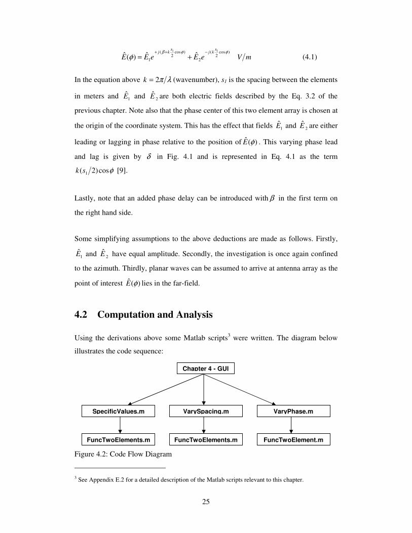
Using the derivations above some Matlab scripts3 were written. The diagram below
illustrates the code sequence:
Figure 4.2: Code Flow Diagram
3 See Appendix E.2 for a detailed description of the Matlab scripts relevant to this chapter.
SpecificValues.m VaryPhase.m VarySpacing.m
Chapter 4 - GUI
FuncTwoElements.m FuncTwoElements.m FuncTwoElement.m

26
The objective of this code was to generate radiation patterns for visualization and
analysis purposes. The GUI (ch4_GUI.m) provides the user with three different
analysis choices, which are achieved by the three scripts SpecificValues.m,
VarySpacing.m and VaryPhase.m. These scripts are in essence plotting functions.
They plot the logarithm of the voltage signal of Eq. 4.1 on a linear decibel grid [1].
The script FuncTwoElements.m is called by each of the three m.files above to
calculate the electric field in the far-field region (using Eq 4.1), for a specific phase
and spacing.
The script SpecificValues.m simply calls FuncTwoElements.m once and plots the
radiation pattern. The input parameters to SpecificValues.m are specified in the GUI.
The script VarySpacing.m is a loop in essence, which calls FuncTwoElements.m as it
loops incrementing spacing between the elements. This script requires a constant
phase value to be set. Again, these input parameters can be set in the GUI. The output
of VarySpacing.m is a surface plot of varying spacing, electric field and azimuth
angle.
Finally, VaryPhase.m is similar to VarySpacing.m, the only difference being that the
phase is incrementally looped while calling FuncTwoElements. This script requires a
constant spacing parameter. Similarly, a surface plot is also generated. The use of a
GUI aids in the quick generation of radiation patterns and enables input parameters to
be changed easily.
4.3 Verification
To verify the code described above comparisons can be made with the radiation
patterns published in the ARRL Antenna Handbook [1]. All the combinations of
spacing and phasing to produce the patterns shown in Fig. C.14 were tested and found
to be in close approximation to the radiation patterns generated by the code. This
served as the necessary verification of the code to generate patterns. As an example
two sets of plots will be compared. 4 See Appendix C for the radiation patterns published in the ARRL Antenna Handbook

27
For the first comparison, a spacing = �/2 and a phase delay = 0 rad is chosen. This is a
well known combination which should illustrate a bidirectional broadside pattern. The
plot generated by the GUI is illustrated in Fig. 4.3(a) and it’s ARRL [1] equivalent is
shown in Fig 4.3(b).
-10
-20
-30
(a) (b)
Figure 4.3: Radiation patterns (spacing = �/2, phase = 0 rad) generated by (a) the simulation GUI and (b) the ARRL [1]. The azimuth angle φ starts at the vertical and proceeds counterclockwise.
Noting that the azimuth angle φ starts at the vertical and proceeds counterclockwise,
refer to Fig. 4.1 to attain a sense of antenna arrangement. Both radiation patterns are
obtained from the logarithm of the voltage in the signal [1]. A slight difference in
these two plots is the log grid. Fig 4.3(a) uses a linear decibel grid known as the
standard log grid [1], where Fig 4.3(b) uses a log grid system of concentric grid lines
spaced periodically [1]. In essence they depict the same relationship and thus by
inspection the two radiation patterns are found equal.
For the second comparison, a spacing of 7/8� and a phase delay of 2π rad was
chosen.
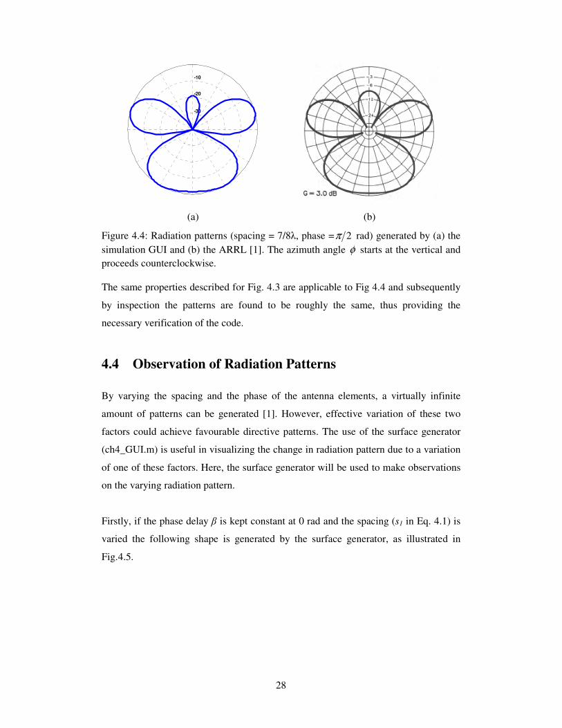
28
-10
-20
-30
(a) (b)
Figure 4.4: Radiation patterns (spacing = 7/8�, phase = 2π rad) generated by (a) the simulation GUI and (b) the ARRL [1]. The azimuth angle φ starts at the vertical and proceeds counterclockwise. The same properties described for Fig. 4.3 are applicable to Fig 4.4 and subsequently
by inspection the patterns are found to be roughly the same, thus providing the
necessary verification of the code.
4.4 Observation of Radiation Patterns
By varying the spacing and the phase of the antenna elements, a virtually infinite
amount of patterns can be generated [1]. However, effective variation of these two
factors could achieve favourable directive patterns. The use of the surface generator
(ch4_GUI.m) is useful in visualizing the change in radiation pattern due to a variation
of one of these factors. Here, the surface generator will be used to make observations
on the varying radiation pattern.
Firstly, if the phase delay � is kept constant at 0 rad and the spacing (s1 in Eq. 4.1) is
varied the following shape is generated by the surface generator, as illustrated in
Fig.4.5.

29
Figure 4.5: Surface of Radiation Pattern due to a varying spacing (0� to 1.5�) between elements.
Noting the colourbar the following observations are made. At a hypothetical zero
spacing the pattern is virtually omnidirectional. As the spacing is increased to 2/λ the
pattern becomes more directive in the directions of 90° and 270° and less so in the
directions 0° (360°) and 180° in the azimuth. Subsequently, at 2/λ the pattern is said
to be broadside, with nulls having formed in the directions of 0° and 180° with
maximum response in the 90° and 270° directions. As the spacing is increased further
to λ1 , sidelobes start to occur at the original position of the nulls at 0° and 180° in the
azimuth. Above λ1 the pattern starts to repeat itself, with the formation of more
sidelobes. This effect is undesirable, as the signal reception becomes ambiguous with
degeneration of directivity. For this reason, spacing of an omnidirectional antenna
array is usually kept below λ1 .
Now, varying the phase β in Eq. 4.1 with respect to a constant spacing, say 2/λ ,
observations are made with reference to Fig. 4.6 below.

30
Figure 4.6: Surface of Radiation Pattern due to a varying phase (0 to 2� rad) between elements. At 0=β rad phase delay, the pattern generated is effectively broadside as described
above. As the phase delay is increased to � rad the radiation pattern changes until its
maximum response is in the azimuth directions 0° (360°) and 180° with nulls having
been formed in the 90° and 270° azimuth directions. The pattern at this phase (� rad)
is known as a bidirectional endfire pattern. Increasing the phase delay further to 2�
rad sees a change of radiation pattern back to its original broadside pattern. An
increase in � above π2 will see a repetition of variation just explained.
4.5 Discussion of Radiation Patterns
This type of variation of phase feed delay can achieve very simple forms of
beamsteering. So, in order to obtain maximum response from a signal in particular
direction it is favourable to orientate the beam (major lobe) formed by the antenna
array, so that it points towards that signal. This is made possible by varying the
element spacing and the added phase delay as shown above.
The radiation patterns were seen to be generally bidirectional. This could become a
drawback as undesirable interference can be easily picked up from behind. Thus
ambiguity may play a significant role when the direction of arrival is important to be
known.

31
4.6 Conclusions
Varying the element spacing and phase delay (within one element) gives rise to many
different patterns. Some of these patterns are more favourable than others, presenting
a more directive radiation pattern, yet directivity is not exceptional in any case due to
the simplicity of the array. Adding a reflector to the system could increase its
directivity.
Furthermore, it would be advantageous to form a null in the direction of a strong
interfering transmitter. The two element array presented here, with variation of
spacing and phase delay is not sufficient to steer nulls, though. This is because nulls
move as a function of spacing and phasing. Thus, fixing of nulls in a particular
direction cannot be achieved in a two element array when beam forming is necessary.

32
Chapter 5
Angle Sensing using Phase Monopulse
This Chapter focuses on monopulse phase sensing techniques for angle measurement.
Using these techniques and the two element array described and discussed in Chapter
4, target tracking will be investigated. In particular, the multiplicative angle sensing
ratio was used as a method to achieve angle measurement of a simulated target [4].
Assumptions were made to simplify the problem. These assumptions will be stated
and reasons for them discussed. Eventually the limitations of this monopulse angle
measurement technique will be investigated and discussed. Matlab was used as the
analysis tool whereby results were calculated.
5.1 Basic Properties and Antenna Arrangement
In general the same structural setup introduced in Chapter 4 will be used with some
minor changes. The antenna arrangement is given below in Fig. 5.1.
Figure 5.1: Antenna and sensing system arrangement
In this chapter the angle γ will be of major importance to the investigation. This
angle γ will indicate the angle of the target of interest from the reference axis y
shown in Fig 5.1. Otherwise, the same setup described in Chapter 4 will be used
φ
γ
y
x
Spacing s1
Target
δ
A B

33
where the spacing between the two elements is represented by the variable s1. The
azimuth angle is φ , and the phase center of the antenna system will be located at the
origin. The half-wave antenna elements are represented by the letters A and B.
5.2 Simplifying Assumptions
Again it is assumed that the target of interest is confined to the azimuthal plane. Also,
it will be assumed that this target follows a circular path around the phase center of
the antenna array at a certain large and constant radial distance. In addition, the wave
arriving at the antenna array is planar as the target will be assumed to be lying in the
far-field region. Yet another core assumption is that the magnitude of the electric field
at each individual element is equal.
5.3 Electric Field Relationships
Using the principle of reciprocity the following deductions were made. The electric
field at the target is given by )(ˆ φE . The electric fields at the antenna elements A and B
are 1E and 2E respectively. As a recap the electric fields at A and B were set up using
the Eq. (3.2).
It must also be reiterated that the amplitudes of 1E and 2E are equal. The relationship
between the electric field at the target and the elements is given by:
)cos2
(
2
)cos2
(
1
11
ˆˆ)(ˆ φφφ
skj
skj
eEeEE−
+= mV (5.1)
This is the same equation used in Chapter 4 if β is disregarded. Again, it can be seen
how the principle of reciprocity is made use of, in the sense that we are interested in
the electric fields received at elements A and B by the target, but in essence they have
already been set up, producing the electric field at the targets position using Eq. 3.2
and 5.1.
A slight modification will be made to the above equation to aid analysis in of in terms
of phase monopulse. The phase advance and delay (shown in Fig. 5.1 as δ ) of the

34
respective elements A and B, receiving a signal from the target, are manipulated to
give5:
δ )sin(21 γs
k= (5.2)
This modification was done in accordance with [4]. Subsequently (5.1) becomes:
)sin2
(
2
)sin2
(
1
11
)(ˆ γγγ
skj
skj
eEeEE−
+= mV . (5.3)
The necessary electric field properties have now been set up.
5.4 Computation and Analysis
The multiplicative angle sensing ratio [4] will be used to determine the relationship
between spacing of elements and angle of arrivalγ . The real output 0q can be shown
to be proportional to γ for small angles ofγ [4] by the equation6:
)sin2
sin(2
12
00 γ
λπsV
q = . (5.4)
Implementing Eq. 5.4 in the Matlab script PhaseMonopulse.m, computes the response
of 0q relative to a variation of γ . The core input parameters listed in Table 3.1 are
used with the addition of a couple others seen, in particular, in Eq. 5.4. 0V is a
constant representing certain amplitudes of signals within the sensing circuit [4] and
will simply be assumed equal to 1. The spacing of elements is set at 21 λ=s and the
angle of arrival is investigated over the range ]90,90[ °°−∈γ .
Subsequently, the relationship between 0q and γ is illustrated in Fig 5.2 below.
5 See Appendix A.1 for detailed derivation 6 See Appendix A.2 for detailed derivation of multiplicative sensing ratio and output response q0

35
Figure 5.2: Relationship between the real output response 0q and angle γ with the reference axis.
The real response can be seen to be sinusoidal, but also note that for small angles
around °= 0γ the response can be approximated proportional. A new variable pγ is
now specified and defined as the angular range over which the response 0q can be
approximated proportional. To find the angular range of pγ , the following
computation was done. Peebles’s deduction for γ small, where λπ 12
0 sVK −= (a
constant), is now used [4]:
γKq −≈1 (5.5)
This relationship between 1q and γ is plotted over the entire range of interest,
]90,90[ °°−∈γ and is presented in Fig. 5.3 as line A.

36
Figure 5.3: The response of 0q (Curve B) and 1q (Line A) as a function ofγ .
The response illustrated in Fig. 5.2 is also shown in Fig. 5.3 as the curve B to give a
visual comparison. Also seen in Fig. 5.3 is an approximation of the proportional
region of curve B in terms of pγ .
The region pγ is of major interest, because the proportional behaviour would allow
one to determine the angle of arrival by measuring a proportional output voltage from
the sensing circuit. Also, it would be preferable for this region to be quite large. A
large pγ would enable tracking of targets over a greater range. Now, to find pγ the
following expression was implemented in the script PhaseMonopulse.m:
errorqq ≤− 01 (5.6)
This equation gives an approximation of the range of pγ within a specified error. The
error for the following calculation will be set at 0.05.
So, fixing the variable 0V and λ of Eq. 5.4 and varying the spacing 1s between
elements A and B would result in a variation of the responses 0q and 1q . Note figure
5.4 below.
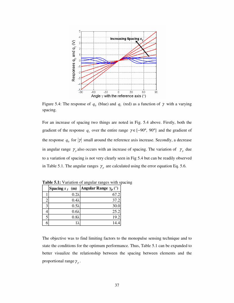
37
Figure 5.4: The response of 0q (blue) and 1q (red) as a function of γ with a varying spacing.
For an increase of spacing two things are noted in Fig. 5.4 above. Firstly, both the
gradient of the response 1q over the entire range ]90,90[ °°−∈γ and the gradient of
the response 0q for γ small around the reference axis increase. Secondly, a decrease
in angular range pγ also occurs with an increase of spacing. The variation of pγ due
to a variation of spacing is not very clearly seen in Fig 5.4 but can be readily observed
in Table 5.1. The angular ranges pγ are calculated using the error equation Eq. 5.6.
Table 5.1: Variation of angular ranges with spacing Spacing s 1 (m) Angular Range �p (°)
1 0.2� 67.22 0.4� 37.23 0.5� 30.04 0.6� 25.25 0.8� 19.26 1� 14.4
The objective was to find limiting factors to the monopulse sensing technique and to
state the conditions for the optimum performance. Thus, Table 5.1 can be expanded to
better visualize the relationship between the spacing between elements and the
proportional range pγ .
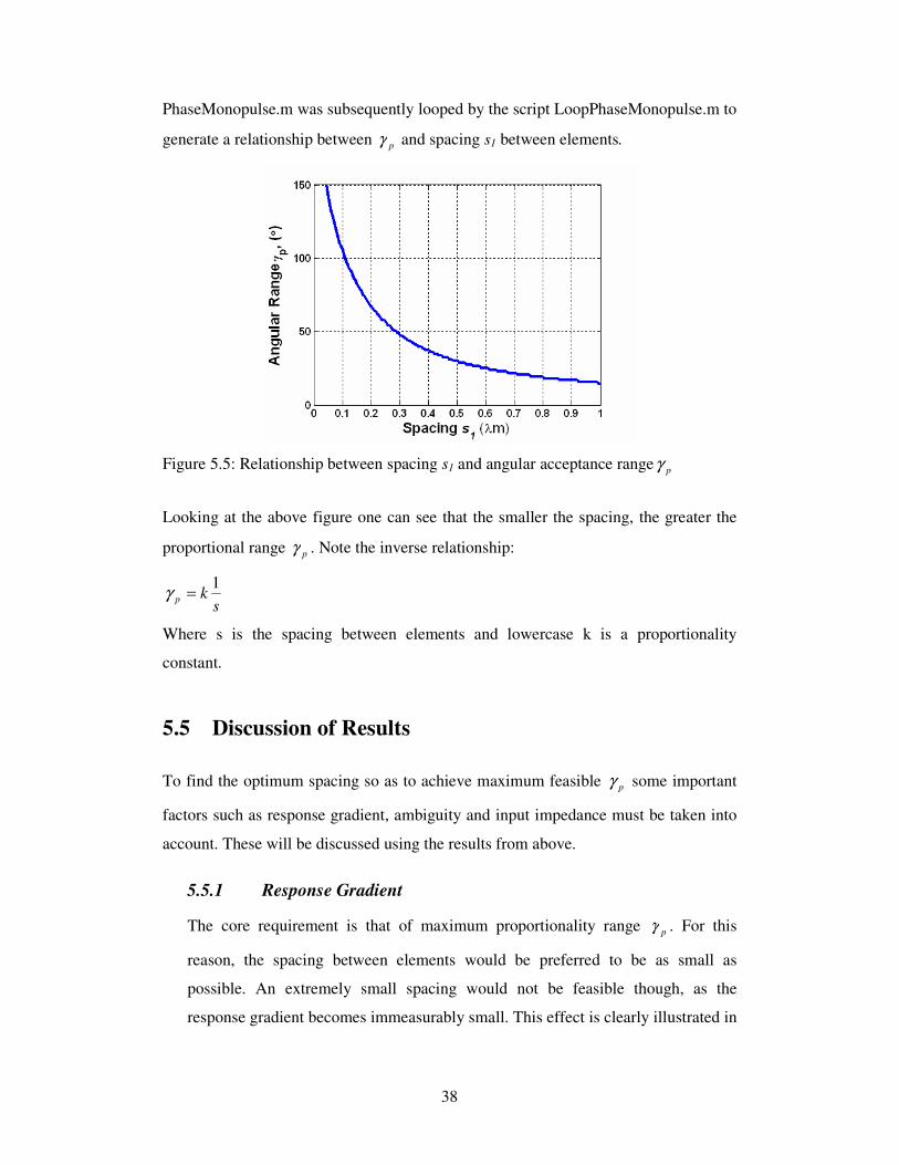
38
PhaseMonopulse.m was subsequently looped by the script LoopPhaseMonopulse.m to
generate a relationship between pγ and spacing s1 between elements.
Figure 5.5: Relationship between spacing s1 and angular acceptance range pγ
Looking at the above figure one can see that the smaller the spacing, the greater the
proportional range pγ . Note the inverse relationship:
skp
1=γ
Where s is the spacing between elements and lowercase k is a proportionality
constant.
5.5 Discussion of Results
To find the optimum spacing so as to achieve maximum feasible pγ some important
factors such as response gradient, ambiguity and input impedance must be taken into
account. These will be discussed using the results from above.
5.5.1 Response Gradient
The core requirement is that of maximum proportionality range pγ . For this
reason, the spacing between elements would be preferred to be as small as
possible. An extremely small spacing would not be feasible though, as the
response gradient becomes immeasurably small. This effect is clearly illustrated in

39
Fig. 5.4, as the spacing between elements is decreased, the gradient approaches
zero.
A small gradient implies that the output response will be difficult to measure due
to a very small output voltage variation. This in turn would cause inaccuracies to
creep in. In particular, it must be noted that the proportional region pγ is based on
an error term (Eq. 5.6), and thus measurements using a small gradient would not
be accurate if the error term is large relative to the measurable output voltage.
5.5.2 Ambiguity of Response
Though a large spacing is unfavourable in terms of pγ it becomes doubly
unfavourable due to the ambiguity of received signal. The radiation pattern of two
element array begins to repeat itself, with an increase of sidelobes. The effect of
repeating signals is most apparent at spacings larger than 1� as was seen in Fig.
4.5. Thus element spacings above 1� will not be considered.
5.5.3 Input Impedance
The input impedance of each element may be considered to be the most important
factor impacting on the optimisation of the system. Fig. B.17 illustrates the
variation of feedpoint impedance with spacing. In general, this graph indicates
that the smaller the element spacing the higher the feedpoint resistance. The graph
requires that each element is parallel, self-resonant and operated in phase [1],
factors that have been satisfied by the simplifying assumptions in this chapter.
Also, it must be noted that for a smaller feedpoint resistance more current will
flow for the same power applied [1], therefore radiating more energy. Looking at
the graph it is apparent that a reasonable region of feedpoint resistance is say less
than 70�. This would imply a spacing range of approximately 0.4� to 0.95�. This
deduction would reduce the maximum possible range of pγ to 37.2°.
7 This figure is found in Appendix B as Figure: B.1.

40
Another important factor is that of mutual impedance. The relationship between
mutual impedance and spacing is shown in Fig. B.28. The region deduced above
for favourable feedpoint impedance, namely 0.4� to 0.95� seems to be a
reasonable region in terms of mutual impedance. Mutual impedance values
become more favourable as the spacing increases. But, conversely these values
become unfavourable below an element spacing of 0.4� due to their large
variations.
5.5.4 The Optimum Monopulse System
Table 5.2 below describes the optimal system in terms of angular range, spacing
and gradient of response.
Table 5.2: The Optimum Monopulse System Spacing s 1 (m) Angular Range �p (°) Gradient of Response
0.4� 37.2 1.20.5� 30.0 1.6
The optimal system setup related to λ4.01 =s , has been determined taking into
account the factors discussed earlier; input impedance, gradient of response and
ambiguity. The spacing 0.5� is also shown in Table 5.2 to compare discrepancies.
Note an angular range discrepancy of 7.2° and greater gradient of response of 0.4
when a spacing 0.5� is used. These are not large differences and thus it may be
preferable to use the spacing of 0.5� as the pattern is well-known and understood.
5.6 Conclusion
Using monopulse sensing techniques for angle measurement was determined to be a
successful method for tracking a target over a specified angular range γ .
Firstly, a favourable spacing range between elements of λ4.01 =s to λ95.0 was
found by investigating the effects of factors such as gradient response, ambiguity,
feedpoint impedance and mutual impedance due to a change of spacing.
8 This figure is found in Appendix B as Figure B.2.

41
Secondly, given this range and a further finding that a smaller element spacing would
provide a greater angular range for tracking of a target, an element spacing of λ5.0
would be a reasonable choice. λ5.0 was chosen over λ4.0 as it’s pattern is well
known and understood. An element spacing of λ5.0 will be regarded as the optimum
element spacing for the optimum monopulse system, which will find further
applications in later chapters.
Further work could be performed in the region of investigating the effect of additional
phase delay and lead in the feed of the antenna elements.
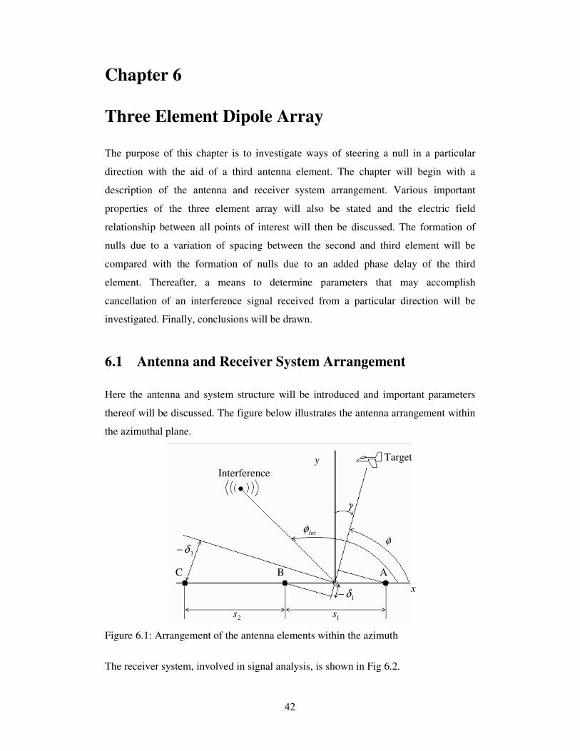
42
Chapter 6
Three Element Dipole Array
The purpose of this chapter is to investigate ways of steering a null in a particular
direction with the aid of a third antenna element. The chapter will begin with a
description of the antenna and receiver system arrangement. Various important
properties of the three element array will also be stated and the electric field
relationship between all points of interest will then be discussed. The formation of
nulls due to a variation of spacing between the second and third element will be
compared with the formation of nulls due to an added phase delay of the third
element. Thereafter, a means to determine parameters that may accomplish
cancellation of an interference signal received from a particular direction will be
investigated. Finally, conclusions will be drawn.
6.1 Antenna and Receiver System Arrangement
Here the antenna and system structure will be introduced and important parameters
thereof will be discussed. The figure below illustrates the antenna arrangement within
the azimuthal plane.
Figure 6.1: Arrangement of the antenna elements within the azimuth
The receiver system, involved in signal analysis, is shown in Fig 6.2.
1δ−
3δ−
Intφ φ
γ
1s 2s
A B C
Target Interference
y
x

43
Figure 6.2: The receiver system represented here as a black box.
With the figures above as a reference the usual and some new simplifying
assumptions are made. Planar waves can once again be assumed as both the point of
interference and the target of interest lie within the far-field region. The target is
assumed to be traveling on a trajectory a constant distance r from the phase center of
the three element array. The interference signal is similarly also placed at a constant
distance r from the phase center.
The variables used in Fig 6.1 will have the same properties as described in Chapter 4
and 5. A new addition in this chapter is the third antenna element denoted as element
C and will also be a half-wave dipole element. It is assumed that the same current
flows at the feed of element C as at the feeds of element A and B. This implies that
the amplitude and magnitude of the electric fields 1E , 2E and 3E at the elements A, B
and C respectively are the same.
Another new addition is the point of interference. This point will be confined to an
azimuth range of ]180,0[ °°∈Intφ . It’s angular position is measured from the x axis.
This is different to the target, whose position is measured from the y axis. Though
some analysis will be done over the entire azimuth range, this chapter will ultimately
be concerned with the ]180,0[ °°∈φ range. The target of interest seen in Fig 6.1 is
not an important part of the analysis of this chapter, but is added for completeness.
The subject of concern in this chapter will lie with the effect the point of interference
has on the antenna array and how this effect can be minimised.

44
Fig. 6.2 shows the basic receiver system which will be concerned with manipulating
signals received by the three antenna elements. In this chapter the manipulation will
simply entail a variation of spacing s2, phase delay β and gain C of the third antenna
element. Its purpose is to achieve nulls in the direction of the point of interference.
After the manipulation has been completed, the signals are summed and the resulting
radiation pattern is investigated.
6.2 The Electric Field Relationships
Some important equations must be presented at this stage. These equations describe
the relationship between the electric fields at the elements, the point of interference
and the target. The core equation to the investigation in this chapter is:
)(ˆ)(ˆ)(ˆˆ 432121321
δδβδδδδ jjjjjjjsum eeeECeeEeeEE −−−− +++++= mV (6.1)
Eq. 6.1 describes the output response shown in Fig. 6.2 and is based on derivation of
Eq. 4.1. The total electric field at each element is given by:
)(ˆˆ 211
δδ jjAelement eeEE += mV (6.2)
)(ˆˆ 212
δδ jjBelement eeEE −− += mV (6.3)
)(ˆˆ 433
δδβ jjjCelement eeeECE −− += mV (6.4)
where 1E , 2E and 3E are calculated using Eq. 3.2 and the phase delays due to spacing
are giving by:
γφδ sin)2(cos)2( 111 sksk Tar == rad (6.5)
Intsk φδ cos)2( 12 = rad (6.6)
γφδ sin))2((cos))2(( 12123 sskssk Tar +=+= rad (6.7)
Intssk φδ cos))2(( 124 += rad (6.8)

45
The variables 1δ and 3δ of Eqs. 6.5 and 6.7 are shown in Fig. 6.1. 2δ and 4δ of Eqs.
6.6 and 6.7 are not shown as this would clutter the diagram, but they can be derived in
the same way as 1δ and 3δ . Using all these equations as a base, null forming was
investigated.
6.3 Null Forming Analysis by Inspection
In this section the formation of nulls due to a variation of spacing s2 and additional
phase delay β will be investigated, by analysing and discussing different graphical
representations.
6.3.1 Computation using Matlab
The analysis to follow was made possible by three Matlab scripts9, namely
ThreeVarySpacing.m, ThreeVaryPhase.m and FuncThreeElements_1.m. The
algorithms within these scripts are based on the equations discussed above.
The script ThreeVarySpacing.m incrementally varies the spacing between the
second and third element. At each increment of spacing s2, the function
FuncThreeElements_1.m is called. This function calculates the electric field in the
far-field region over the entire azimuth range. Once the loop is complete
ThreeVarySpacing.m determines the radiation pattern and plots it in the form of a
surface. The surface is plotted relative to the entire azimuth range and the change
of element spacing s2.
In the same way ThreeVaryPhase.m calculates the change of the radiation pattern
over a change in additional phase delay β in the third element as shown in Fig
6.2. FuncThreeElements_1.m is also called by this script to determine the electric
field in the far-field region. As above, ThreeVaryPhase.m also illustrates the
radiation pattern by plotting it in the form of a surface.
9 See Appendix E.4 for a detailed description of the Matlab scripts of this chapter
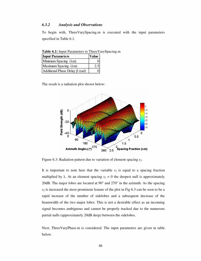
46
6.3.2 Analysis and Observations
To begin with, ThreeVarySpacing.m is executed with the input parameters
specified in Table 6.1.
Table 6.1: Input Parameters to ThreeVarySpacing.m Input Parameters ValueMinimum Spacing (�m) 0Maximum Spacing (�m) 2.5Additional Phase Delay � (rad) 0
The result is a radiation plot shown below:
Figure 6.3: Radiation pattern due to variation of element spacing s2.
It is important to note here that the variable s2 is equal to a spacing fraction
multiplied by �. At an element spacing s2 = 0 the deepest null is approximately
20dB. The major lobes are located at 90° and 270° in the azimuth. As the spacing
s2 is increased the most prominent feature of the plot in Fig 6.3 can be seen to be a
rapid increase of the number of sidelobes and a subsequent decrease of the
beamwidth of the two major lobes. This is not a desirable effect as an incoming
signal becomes ambiguous and cannot be properly tracked due to the numerous
partial nulls (approximately 20dB deep) between the sidelobes.
Next, ThreeVaryPhase.m is considered. The input parameters are given in table
below.

47
Table 6.2: Input Parameters of ThreeVaryPhase.m Input Parameters ValueMinimum phase delay � (rad) 0Maximum phase delay � (rad) 2�Spacing s2 (m) 0.5�
Running the script ThreeVaryPhase.m the following radiation pattern is produced.
Figure 6.4: Radiation pattern to a change in the phase delay � of the third element.
At phase delay � = 0 rad the major lobes are at azimuth angles of 90° and 270°,
with the deepest nulls found on either side of these major lobes. As � is increased
to � rad the major lobes begin to skew towards a azimuth direction of 0° (360°)
while at the same time two new lobes appear in the opposite direction,
symmetrical about azimuth angle 180°. At � rad there are four relatively large
lobes in the pattern. A further increase � sees a decrease in magnitude of the two
original major lobes and a skewing of the two new lobes towards the 90° and 270°
directions, putting the pattern back in its original state. This process would be
repeated if � were increased above 2� rad.
To view any particular combination of phase delay � and spacing s2 as described
above in a 2-D plot, the script ThreeElements.m can be used.

48
6.3.3 Conclusion
With reference to the diagrams above the following conclusion are drawn. Large
values of spacing s2 would be very unfavourable due to a rapid increase of
sidelobes. Futhermore, the increase of sidelobes decreases the beamwidth of the
major lobes, which is also undesirable in terms of target tracking. The radiation
pattern produced by varying the phase delay � while keeping the s2 constant did
not show the serious degradation effects that an increase of spacing s2 did. In
particular, Fig 6.2 did not show any increase of sidelobes over its entire range.
For this reason, it can be concluded that when attempting null formation, a
variation of phase delay will be preferred over a variation of spacing s2.
In addition, there is a practical advantage of relying solely on phase (and gain)
variation, namely one would not need to physically move any antenna hardware as
variation of phase (and gain) can be done electronically.
Finally, due to the fact that a large spacing of s2 has undesirable effects, it will be
set to 0.5 λ . Furthermore, from here on null formation will be investigated by
varying only the phase and gain of element C as shown in Fig. 6.2.
6.4 Optimum Parameter Calculation
The focus of this investigation is to determine the parameters of phase delay � and
gain C in order to create a pattern that forms a null in a particular direction. The
element spacing s2 will be kept constant at 2/λ due to the undesirable effects of its
sidelobe build up at large spacings as found in the section above.
6.4.1 Computation of Parameters
The parameters of phase delay � and gain C are calculated by a Matlab script
called ParameterCalc.m. Once these two parameters have been found, the script
calls the function FuncThreeElements_2.m. FuncThreeElements_2.m must not be
confused with FuncThreeElements_1.m of the above section. These functions
have different input arguments. FuncThreeElements_2.m is a function that

49
calculates the radiation pattern of the antenna array for the calculated parameters
phase � and gain C. The depth of the null and maximum response at 90° to the
array axis (positive x axis) is also calculated in FuncThreeElements_2.m.
The Eq. 6.1 is modified as follows so as to determine the minimum possible
response for an angle at which the point of interference is expected. The
interference signals induced in elements A and B are of major interest. It is
preferable that these are made as small as possible. To achieve this, the gain and
phase delay must be chosen accordingly.
To this end Eq. 6.1 was reduced to:
)(ˆ)(ˆ)(ˆˆ 422321
δβδδ jjjjTotInt eeECeEeEE −− ++= mV (6.9)
which represents a summation of all the interfering signals in all the elements.
ParameterCalc.m calculates TotIntE for a variation of gain C and phase � for a point
of interference at a specific angle Intφ . It then proceeds by finding the minimum
magnitude of TotIntE and the associated C and � parameter values. As stated
earlier, these values are then fed into FuncThreeElements_2.m providing the
output radiation plot which illustrates that any signal coming from the specified
interference position would be nulled.
6.4.2 Analysis of Radiation Patterns
Running the script files for variety of interference positions allows a number of
interesting observations to be made. Spacings s1 and s2 as described in Fig 6.1 will
remain constant at 2/λ throughout this investigation.
To begin with, two radiation patterns will be generated to illustrate null formation
at particular positions.

50
Figure 6.5: Radiation patterns with the interference point specified °= 140Intφ
The above figure illustrates a radiation pattern that was generated by simply
inputting the angle of interference. The angle of interference is measured from the
x axis. The information relevant to the above figure and found by running the
script ParameterCalc.m is listed in Table 6.4.
Table 6.3: Properties related to Fig. 6.5 found by ParameterCalc.m Value
Interference Angle �int (°) 140Gain C 0.72Phase Delay � (rad) 5.81Null Depth (dB) -98.66Max Response at 90° (dB) -0.09
The null depth at 140° seems to be very reasonable, and maximum response at 90°
to the x axis is also only 0.09 dB below the normalized maximum. Thus using the
parameters of C and � to manipulate the signal in the third element would result in
a system that effectively reduces interference from an angle of =Intφ 140° but yet
still has a good response for signals arriving from the broadside direction, at
=φ 90° from the x axis.
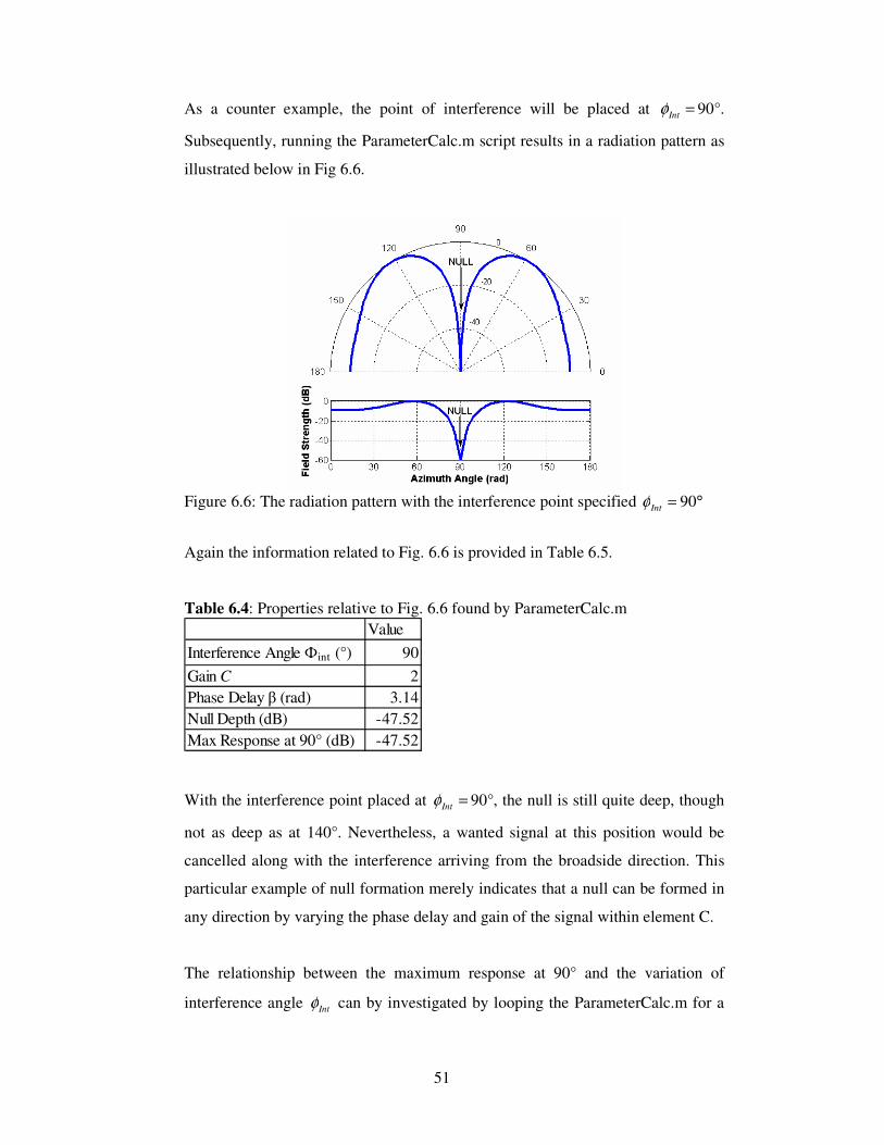
51
As a counter example, the point of interference will be placed at =Intφ 90°.
Subsequently, running the ParameterCalc.m script results in a radiation pattern as
illustrated below in Fig 6.6.
Figure 6.6: The radiation pattern with the interference point specified °= 90Intφ
Again the information related to Fig. 6.6 is provided in Table 6.5.
Table 6.4: Properties relative to Fig. 6.6 found by ParameterCalc.m Value
Interference Angle �int (°) 90Gain C 2Phase Delay � (rad) 3.14Null Depth (dB) -47.52Max Response at 90° (dB) -47.52
With the interference point placed at =Intφ 90°, the null is still quite deep, though
not as deep as at 140°. Nevertheless, a wanted signal at this position would be
cancelled along with the interference arriving from the broadside direction. This
particular example of null formation merely indicates that a null can be formed in
any direction by varying the phase delay and gain of the signal within element C.
The relationship between the maximum response at 90° and the variation of
interference angle Intφ can by investigated by looping the ParameterCalc.m for a

52
range of interference angles. This is done by a slightly modified script called
ParameterCalcLoop.m. This relationship can be seen in Fig .6.7.
Figure 6.7: Relationship between Max Response at 90° and Interference Angle
Intφ This graph presents an interesting relationship in the sense that the response in the
broadside direction or at 90° counterclockwise from the x axis is at maximum for
a very wide range of interference. For instance, if -6dB is considered an
unacceptable drop in response gain, it is found that the range ]106,74[ °°∈φ is
the only unfavourable range as shown on the graph. And conversely, the response
gain in the broadside direction is relatively large (above -6dB) for all interference
positions outside the range ]106,74[ °°∈φ .
An assumption is now made that the interference signal will not pass over the
region used for angle sensing as described in Chapter 5. This implies that nulls
can freely and effectively be place in the range outside ]106,74[ °°∈φ without
having any undesirable effects on the reception of the target signal.

53
6.4.3 Conclusion
The results show that a sufficient null depth can be achieved with correct phasing
and gain variation for any interference angle Intφ . Furthermore, with the
assumption that the interference signal will never arrive from the angular range
allocated for angle sensing, the response from that range can be expected to be
very high, namely above -6dB of the normalized field strength.

54
Chapter 7
Phase Monopulse Sensing with added
Interference
The purpose of this chapter is to investigate ways in which monopulse angle sensing
can be achieved with the presence of an interfering signal. The third element,
introduced in Chapter 6, will be used to attempt a cancellation of the interference
within the first and second antenna elements by means of changing the phase delay
and gain of the incoming signal in element C. The chapter will begin with a
description of the receiving system used. Monopulse angle sensing techniques will
then be applied to the first two elements as was done in Chapter 5, starting with a
situation where no attempt to cancel the interference is made. Thereafter, partial
interference canceling will be dealt with and then finally full interference canceling
will be investigated. Matlab was used as a tool whereby results were computed.
7.1 Receiver System Arrangement
The properties introduced and discussed in Chapter 6 regarding antenna arrangement,
particularly Fig 6.1, are also applicable here. In this chapter more emphasis will be
placed on the angle γ , the angle to the target of interest from the reference axis y. A
significant change in this chapter from the last will be in terms of the receiver system.
The black box will now manipulate signals as indicated in Fig 7.1.
Figure 7.1: Receiver system used to manipulate signals

55
The investigation to follow in this chapter will all begin with the spacings s1 and s2
fixed at 0.5 λ . The only factors to be varied will be the gain parameters G, H and
phase delays σ ,ε shown in Fig. 7.1. The idea here is that the interference received in
elements A and B will be cancelled out before monopulse angle sensing is applied.
The process of monopulse angle sensing makes use of the multiplicative angle sensing
ratio and is shown in the Fig 7.1 as the multiplication sign between the two incoming
channels.
7.2 Investigation of Signals Received
The Eqs. 6.1 through 6.8 also apply to the antenna and receiver system described
above. Looking at Fig 7.1 it is noted that in order to achieve a situation where the
signals after the summation points are free of interference, the signal from element C
must be added in such a way so as to minimize the interference received in elements
A and B. In terms of signal manipulation two equations will form the basis of the
investigations to following this chapter. These equations were derived from Eqs. 6.1
through 6.8.
)(ˆˆˆˆ 43213111
δδεδδ jjjjInt
jTarCLEAN eeeEHeEeEE −− +++= mV (7.1)
)(ˆˆˆˆ 43213222
δδσδδ jjjjInt
jTarCLEAN eeeEGeEeEE −−−− +++= mV (7.2)
Where CLEANE1ˆ and CLEANE2
ˆ represent the signals after the summation in the
respective channels. G, H are gain values and σ ,ε are phase delays as described in
Fig. 7.1. The remaining variables of the above equations are discussed in Chapter 6.
7.3 Computation of Interference Cancellation
The first of the three investigations to be performed in this chapter will investigate
monopulse angle sensing under the condition that no interference canceling will be
done. This implies that the gain values of H and G in either channel will be set to zero
thus canceling any effect of the third element. The Matlab script written to investigate
this is called NoIntCancel.m.

56
The second investigation is performed by PartialIntCancel.m. This script calculates
the minimum possible interference components in either channel such that the last two
terms on the right of Eqs. 7.1 and 7.2 are at a minimum.
The third investigation assumes that element C is a directive antenna. This implies
that the term related to 3δje− (found in the brackets on the right side of Eqs. 7.1 and
7.2) within the third element can be assumed zero. This term describes the phase
delay induced in element C by the target signal. In theory this method should give an
even better response than that of the PartialIntCancel.m.
All these m.files10 call the function CH7_PhaseMonopulse.m to perform the phase
monopulse calculation.
Running each of the three scripts provides a graphical representation of the response
similar to the one in Chapter 5. This allows comparisons to be made between the two.
These graphical representations will once again form the basis of the analysis.
Furthermore, the analysis will be done progressively beginning with NoIntCancel.m,
which is followed with PartialIntCancel.m and finally ending with FullIntCancel.m.
7.4 No Interference Cancellation
This section investigates the implications of performing angle sensing monopulse on
the two signals in channels 1 and 2 where no interference cancellation has been done.
7.4.1 Computation and Analysis
As mentioned, if no interference cancellation is attempted, G and H will be set to
zero. This has the effect that monopulse sensing will be done on the signals in
channel 1 and 2 that contain the complete signal components from both the target
and interference. Eqs 7.3 and 7.4 below are derived from Eqs. 7.1 and 7.2.
21111
ˆˆˆ δδ jInt
jTarCLEAN eEeEE += mV (7.3)
10 See Appendix E.5 for a detailed description of the Matlab script relevant to this chapter

57
21222
ˆˆˆ δδ jInt
jTarCLEAN eEeEE −− += mV (7.4)
Applying phase monopulse sensing techniques to these to signals results in the
following relationship illustrated in Fig. 7.2.
Figure 7.2: Responses q0 and q1 relative to the angle γ of the target, under the condition of no interference cancellation
From this figure it can clearly be seen that a large error in angle reading will
occur. Firstly, there is no proportional region. Secondly, there is an offset from the
origin in the order of -0.4V. Thus, broadside to the antenna array or if γ were
equal to 0° then the output of the system would give -0.4V. Using this voltage and
the linear approximation shown by line A as a reference, the target will be
estimated at an angle 15° counterclockwise from the reference axis. This error
would be unacceptable.
7.4.2 Conclusion
All in all, if the interference is not canceled in each channel no phase monopulse
sensing can be done. In order for this system to work the real response q0 must
pass through the origin and there must also be a reasonable range over which the
response is proportional to the linear approximation q1. But as can be seen this is
not the case and thus another approach must be investigated.

58
7.5 Partial Interference Cancellation
For a variation of target position the parameters G, H and σ ,ε of Eqs. 7.1 and 7.2 are
calculated with the objective of minimizing the interference components in channels 1
and 2 so that monopulse angle sensing can be performed with better results than as
found above.
7.5.1 Computation and Analysis
Varying the target’s position in the azimuth for ]90,90[ °°−∈γ the parameter
values were calculated using a reduced version of Eqs. 7.1 and 7.2, namely:
)(ˆˆˆ 432311
δδεδ jjjjIntINTC eeeEHeEE −− ++= mV / (7.5)
)(ˆˆˆ 432322
δδσδ jjjjIntINTC eeeEGeEE −−− ++= mV / (7.6)
INTCE 1ˆ and INTCE 2
ˆ above represent the total interference components in channels
1 and 2 respectively. For each position of the target in the range of γ a range of
gain values (G and H) and a range of phase delays (σ and ε ) forming a matrix
were tested to find the minimum possible magnitudes for INTCE 1ˆ and INTCE 2
ˆ .
Table 7.1 represents these and other important input parameters specific to the
Matlab script ParitalIntCancel.m.
Table 7.1: Input Parameters of PartialIntCancel.m Value
Range of Target Position � (°) � [-90°, 90°]Range of Gain G, H � [0, 4]Range of Phase Delay �, � (rad) � [0, 2�]Interference Position �Int (°) 135°
Spacings s1 and s2 �/2 Refer to Fig 6.1 for a recap on the properties of spacings s1 and s2 and interference
position �Int.
Running PartialIntCancel.m with the values specified in Table 7.1, results in the
following. First off, the parameters G, H, σ and ε for the minimum possible

59
magnitudes for INTCE 1ˆ and INTCE 2
ˆ (or maximum interference cancellation) are
found and presented in the Fig. 7.3 and 7.4.
Figure 7.3: Phase delay values σ (red) and ε (black) for minimum possible interference over the target range �.
Figure 7.4: Gain values G (red) and H (black) for minimum possible interference over the target range γ .
Two things can be noted when considering Fig 7.3. Firstly, there is a constant
phase difference between the values of the two phase delays as indicated on the
figure. Secondly, at °= 0γ there is a π rad jump in the phases as the target crosses
the broadside position. This jump is due to the output response q0 crossing the
zero point.
In terms of gain, the Fig. 7.4 shows that the two values of G and H are equal for
the entire range of target position. Also, as the target moves over, or looking more
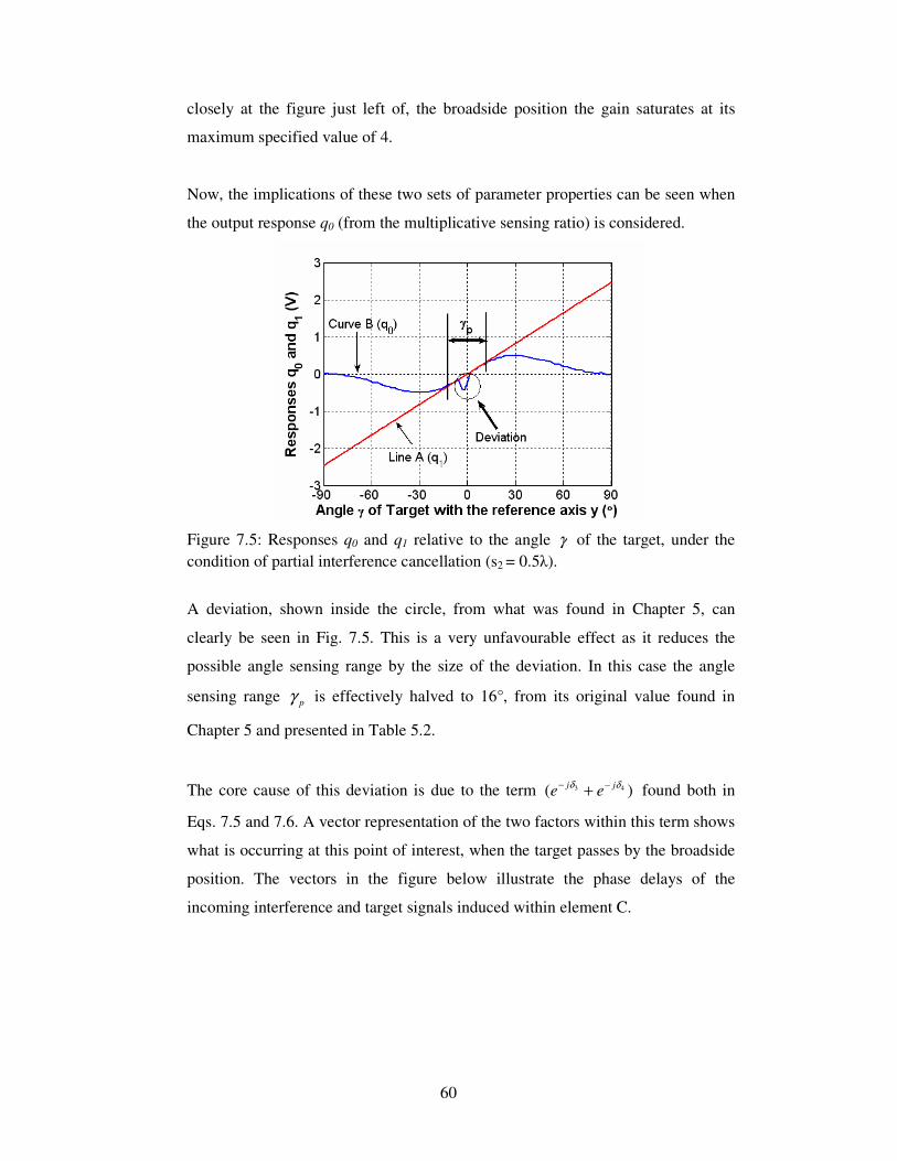
60
closely at the figure just left of, the broadside position the gain saturates at its
maximum specified value of 4.
Now, the implications of these two sets of parameter properties can be seen when
the output response q0 (from the multiplicative sensing ratio) is considered.
Figure 7.5: Responses q0 and q1 relative to the angle γ of the target, under the condition of partial interference cancellation (s2 = 0.5�).
A deviation, shown inside the circle, from what was found in Chapter 5, can
clearly be seen in Fig. 7.5. This is a very unfavourable effect as it reduces the
possible angle sensing range by the size of the deviation. In this case the angle
sensing range pγ is effectively halved to 16°, from its original value found in
Chapter 5 and presented in Table 5.2.
The core cause of this deviation is due to the term )( 43 δδ jj ee −− + found both in
Eqs. 7.5 and 7.6. A vector representation of the two factors within this term shows
what is occurring at this point of interest, when the target passes by the broadside
position. The vectors in the figure below illustrate the phase delays of the
incoming interference and target signals induced within element C.

61
Figure 7.6: Vector representation of phase delays of the target ( 3δ ) and interference ( 4δ ) signals
The interference vector remains constant at the position indicated for the values
specified in Table 7.1. As the target traverses its trajectory over the range
]90,90[ °°−∈γ its phasor passes directly opposite to the interference phasor as
shown in Fig.7.6. This causes the term )( 43 δδ jj ee −− + to become infinitely small
and in response to this the gains G and H increase as seen in Fig. 7.4. However,
both gains are limited to a finite value of 4 and are unable to compensate for the
deviation. The implications of this are such that second terms on the right hand
side of Eqs. 7.5 and 7.6 tend to zero leaving the interference components of
21
ˆ δjInteE and 2
2ˆ δj
InteE − in channels 1 and 2 intact.
To counteract this degrading effect the spacing s2 between elements B and C can
be slightly varied. Keeping in mind the unfavourable effects of large spacings of
s2 found in Chapter 6, s2 is now set to 0.9�. Following the same procedure as
before, the output response q0 is found and shown in Fig. 7.7 below.

62
Figure 7.7: Responses q0 and q1 relative to the angle γ of the target, under the
condition of partial interference cancellation (s2 = 0.9�).
Having changed s2 to 0.9�, the proportional range described by pγ is seen to be
free of any major degrading deviations. The degrading deviation has moved to the
indicated position outside the proportional range pγ , restoring pγ to its original
value of 30°.
Another observation that can be made by looking at Fig. 7.7 is that the response q0
seems to be noisy inside the range pγ . Despite this effect, the relationship
presented in Fig. 7.7 still satisfies the error term described by Eq 5.6.
7.5.2 Conclusion
These findings presented a method of canceling interference in channels 1 and 2
for the purpose of monopulse angle measurement. This method proved successful,
but required a variation of a number of parameters for accurate tracking of a
target. This is not entirely favourable, as such a system would require significant
signal analysis and control systems. Furthermore, undesirable noise seemed to be
present in the output response, but was concluded to be inconsequential.

63
7.6 Full Interference Cancellation
The final investigation is based on the assumption that element C is a directive
antenna element. This implies that the antenna can be positioned in such a way as to
solely pick up the interfering signals.
7.6.1 Computation and Analysis
Applying the idea of directivity, the term ( 3δje− ) in Eqs. 7.5 and 7.6 is set to zero
so as to get:
)(ˆˆˆ 42311
δεδ jjjIntINTC eeEHeEE −+= mV / (7.7)
)(ˆˆˆ 42322
δσδ jjjIntINTC eeEGeEE −− += mV / (7.8)
The same procedures followed in the previous section will once again be followed
here. The goal as before, is to find the parameter values of G, H, σ and ε so as
obtain the minimum possible magnitudes of INTCE 1ˆ and INTCE 2
ˆ .
The same input parameters as stated in Table 7.1 will be used. Now, running the
script FullIntCancel.m returns the following results in terms of G, H, σ and ε .
(a) (b)
Figure 7.8: Parameter values of (a) phase delays (σ and ε ) and (b) Gain (G and H) for minimum possible interference for FullIntCancel.m
Fig. 7.8 shows constant values for all parameter values. The parameters associated
with channel 1 (H,ε ) are given in black and the parameters associated with
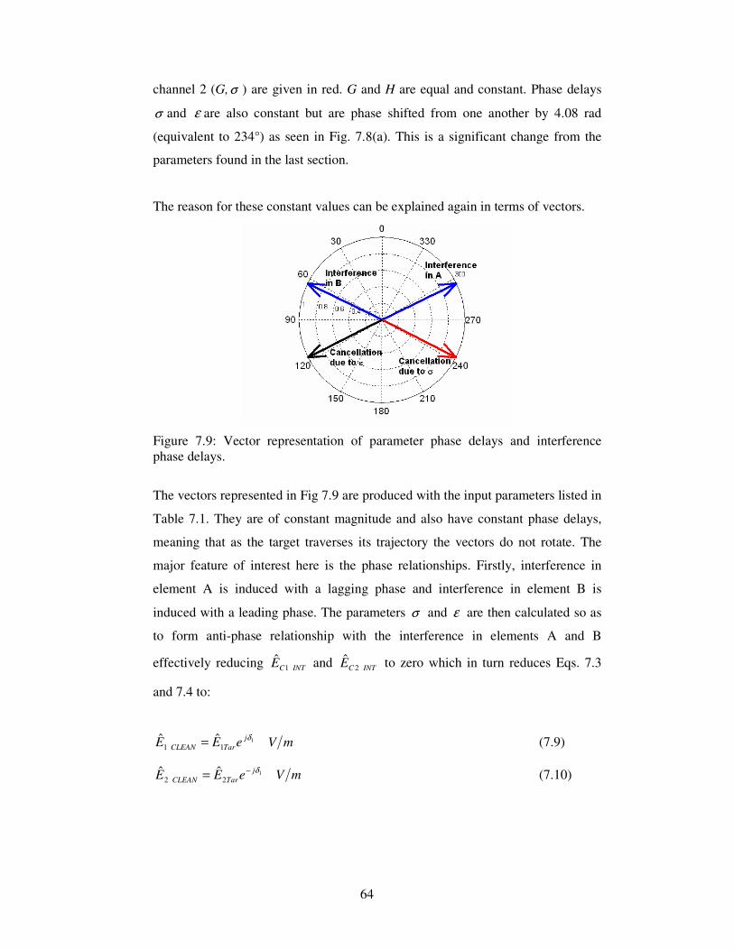
64
channel 2 (G,σ ) are given in red. G and H are equal and constant. Phase delays
σ and ε are also constant but are phase shifted from one another by 4.08 rad
(equivalent to 234°) as seen in Fig. 7.8(a). This is a significant change from the
parameters found in the last section.
The reason for these constant values can be explained again in terms of vectors.
Figure 7.9: Vector representation of parameter phase delays and interference phase delays.
The vectors represented in Fig 7.9 are produced with the input parameters listed in
Table 7.1. They are of constant magnitude and also have constant phase delays,
meaning that as the target traverses its trajectory the vectors do not rotate. The
major feature of interest here is the phase relationships. Firstly, interference in
element A is induced with a lagging phase and interference in element B is
induced with a leading phase. The parameters σ and ε are then calculated so as
to form anti-phase relationship with the interference in elements A and B
effectively reducing INTCE 1ˆ and INTCE 2
ˆ to zero which in turn reduces Eqs. 7.3
and 7.4 to:
111
ˆˆ δjTarCLEAN eEE = mV (7.9)
122
ˆˆ δjTarCLEAN eEE −= mV (7.10)

65
To observe the implications of this behaviour, monopulse sensing is performed on
the two signals CLEANE1ˆ and CLEANE2
ˆ coming out of the summation blocks of Fig.
7.1. The result is seen in Fig 7.10.
Figure 7.10: Response of 0q and 1q for a variation of target angle γ , under the condition of full interference cancellation
Fig. 7.10 shows a very clean response of 0q , much like the response found in
Chapter 5. Calculating the angular range of pγ over which the response 0q is
proportional finds °= 6.30pγ . This relates very closely with the value found in
Chapter 5 in Table 5.2 for an element spacing s1 = 0.5�.
7.6.2 Conclusion
The condition of full interference cancellation where the third antenna element is
assumed directive was found to be very successful for angle measurement. This
method does not present the unfavourable effects of deviations and noise that were
found under the condition of partial interference cancellation. Consequently, this
is the most desirable method when angle measurements are to be taken using
phase monopulse techniques.

66
Chapter 8
Conclusions and Future Work
This thesis investigated the feasibility of a number of methods and techniques to
achieve beam forming and null placement, with the ultimate goal of target tracking.
The properties, favourable and unfavourable, of these methods and techniques were
analysed and discussed in detail to determine optimum antenna system parameters.
The establishment of a firm literary base was believed important. Thus to this end, a
great deal of literature was studied and reviewed and ultimately presented in Chapter
2 of this thesis.
The actual analytical work done in this thesis began by setting a foundation with an
investigation into a single omnidirectional half-wave dipole element. The addition of
a second identical antenna element showed the possibility of simple beam forming
with a variation of phasing and spacing of the two elements. Though, at the same time
it was found that a fixed null could not be placed in one particular direction while
beam forming was taking place.
Using monopulse sensing techniques [4] for angle measurement was determined to be
a successful and effective method for tracking a target over a specified angular range.
This range is desired as large as possible but is constrained by factors of gradient
response, ambiguity and input impedance. Subsequently, the optimum monopulse
system for a two element array was determined to be at an element spacing of 0.5 λ .
The addition of a third antenna element to the array, provided a means of steering a
null in any particular direction while keeping a reasonable response in the broadside
direction. Furthermore, the addition of the third element enabled monopulse sensing
techniques to successfully track a target signal despite the presence of an added
interfering signal. In particular, the case of using a directive third antenna element for
interference canceling in a monopulse system proved to be indeed the most desirable
and optimal method investigated for target tracking in this thesis.

67
In terms of future work, much additional analytical work can be done to further the
investigations begun in this thesis. In particular, the investigations done in Chapter 7
can be furthered by looking into possible applications to a practical system. This said,
the work done in this thesis was purely of an analytical nature. Subsequently, all the
investigations and analyses carried out here could be verified by practical
implementation.

68
Appendix A: Derivations
A.1: Derivation 1
δ φcos21s
k= )2
cos(21 γπ −= s
k = )sin(21 γs
k
The above equation is represented in the text as Eq. 5.2
A.2: Derivation 2
According to Peebles the one-way complex receiving voltage pattern is specified as
[4]:
)()()( γβγγ jefp = .
See Chapter section 2.3.2 on pattern representation to see how this expression was
derived. The multiplicative angle sensing ratio was defined as [4]:
)(2
)()(
)( γβ
γγγ j
m epp
r =−
= .
Following the deduction of Peebles a complex voltage R is found to be [4]:
)(2
20 γmr
jVR
−= .
Using the expressions above the real output 0q of the complex response R above can
be shown to be proportional to γ for small angles ofγ [4]. I.e.:
)sin2
sin(2
)Re( 12
00 γ
λπsV
Rq == .
The above expression is represented in the text as Eq. 5.4.
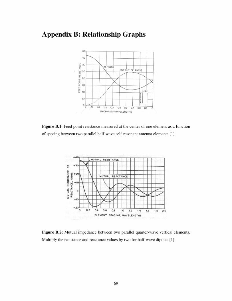
69
Appendix B: Relationship Graphs
Figure B.1: Feed point resistance measured at the center of one element as a function
of spacing between two parallel half-wave self-resonant antenna elements [1].
Figure B.2: Mutual impedance between two parallel quarter-wave vertical elements.
Multiply the resistance and reactance values by two for half-wave dipoles [1].

70
Appendix C: The ARRL Radiation Patterns [1]
Figure C.1 (a)

71
Figure C.1 (b)
Figure C.1: Azimuth (H-plane) patterns of two identical parallel driven elements,
spaced and phased as indicated (S = spacing, φ = phasing). The elements are aligned
with the vertical (0°, -180°) axis, and the element nearer the 0° direction (top of the
page) is of lagging phase at angles other than 0°. The two elements are assumed to be
thin and self-resonant, with equal-amplitude currents flowing at the feed point. The
plots represent the free-space vertical or elevation pattern of two horizontal half-wave
elements when viewed on end, with one element above the other [1].

72
Appendix D: Makarov Code Sequence Diagram
[5]
Figure D.1: Flowchart of the complete radiation algorithm [5]

73
Appendix E: Matlab Code Description
The Matlab scripts written for this thesis are found on the CD provided. All the
m.files presented in each chapter are located in separate folders. For instance, the
Matlab scripts of used in Chapter 5 are found in a folder on the CD called Chapter5.
This appendix lists all the m.files contained in each chapter folder and gives a brief
description. The descriptions are also found in the actual scripts.
E.1 - Chapter 3 Single Half-Wave Antenna Element
The following Matlab scripts are found in the folder Chapter3 on the CD provided.
Relevant Scripts: SingleElement.m
Description: SingleElement.m:
This Matlab script is a stand alone script that calculates the amplitude radiation
pattern.
E.2 - Chapter 4 Two Element Dipole Array
The following Matlab scripts are found in the folder Chapter4 on the CD provided.
List of Scripts TwoElements.m
Ch4_GUI.m
SpecificValues.m
VarySpacing.m
VaryPhase.m
FuncTwoElements
74
Description TwoElements:
This m.file builds on SingleElement.m. Here a second half-wave dipole element is
added. The purpose of this m.file is to investigate the effects of a change of spacing
and phasing between two elements on the radiation pattern. The calculation of the
electric fields is based on 4.1 in the thesis.
ch4_GUI.m:
This m.file provides a graphical user interface to enable the user to input parameters
of spacing and phasing easily and quickly. This GUI calls upon three other m.files,
namely, VarySpacing.m, VaryPhase.m and SpecificValues.m. It provides the user
with the option of producing a surface of a varying parameter or of producing a single
plot with specific parameters.
SpecificValues.m:
This function is called by ch4_GUI. It itself calls the FuncTwoElements.m function
and plots the calculated electric field of two elements in a polar and rectangular
coordinate system.
VarySpacing.m:
This function is called by ch4_GUI.m. It calculates the electric field by calling the
function FuncTwoElements.m. Finally, it illustrates the radiation pattern over the
entire azimuthal range as a function of varying spacing at a constant specified feed
phase.
VaryPhase.m:
This function is called by ch4_GUI.m. It calculates the electric field by calling the
function FuncTwoElements.m. Finally, a surface is plotted that illustrates the
radiation pattern over the entire azimuthal range as a function of varying feed phase in
one of the two antenna elements at constant specified spacing between the two
antenna elements.

75
FuncTwoElements.m:
This m.file is a function and is called by SpecificValues.m, VarySpacing.m and
VaryPhase.m (these 3 are all functions), all of which are called by the ch4_GUI.m.
FuncTwoElements.m calculates the electric field in the far-field region. This is done
so as to plot various radiation patterns.
E.3 - Chapter 5 Angle Sensing Using Phase Monopulse
The following Matlab scripts are found in the folder Chapter5 on the CD provided.
List of Scripts PhaseMonopulse.m
LoopPhaseMonopulse.m
FuncPhaseMonopulse.m
Description PhaseMonopulse.m:
This m.file uses phase monopulse to determine the angle of arrival of a target and also
the effective range over which a target can be accurately tracked. In particular the
multiplicative angle sensing ratio was used [4].
LoopPhaseMonopulse.m:
The purpose of this m.file is to calculate the proportional range of the output response
q0. This proporitonal range describes the range over which the target's angle can
accurately be sensed. The result is visualised with the aid of a graph of pγ vs element
spacing s1.
FuncPhaseMonopulse.m:
This m.file is a function that is called by LoopPhaseMonopulse.m. The purpose of this
function is to calculate the angular range over which the response q0 is proportional.
E.4 - Chapter 6 Three Element Dipole Array
The following Matlab scripts are found in the folder Chapter6 on the CD provided.

76
List of Scripts ThreeElements.m
ThreeElementsCheck.m
ThreeVarySpacing.m
ThreeVaryPhase.m
FuncThreeElements_1.m
ParameterCalc.m
ParameterCalcLoop.m
FuncThreeElements_2.m
Description: ThreeElements.m:
This m.file builds on TwoElements.m. Here a third half-wave dipole element has been
introduced. The purpose of this m.file was to investigate the effects of spacing and
phasing of the third element on the radiation pattern.
ThreeElementsCheck.m:
This m.file was written to check the output of ThreeElements.m. It can only check
ThreeElements.m for constant spacing between elements, and thus is only useful once
off. The equation used in this script was found in the Antenna Design Handbook [9].
ThreeVarySpacing.m:
This m.file calls FuncThreeElements_1.m to calculate the electric field which it then
illustrates over the entire azimuthal range as a function of varying spacing of the third
dipole element (C). The first two antenna elements (A and B) have a constant element
spacing.
ThreeVaryPhase.m:
This m.file calls FuncThreeElements_1.m to calculate the electric field which it then
illustrates over the entire azimuthal range as a function of varying phasing of the third
dipole element. It plots the logarthim of the voltage in the signal. The first two
antenna elements have constant element spacing and are not shifted in phase by an
additional phase shift.

77
FuncThreeElements_1.m:
This function is called by the m.files ThreeVarySpacing.m and ThreeVaryPhase.m. It
calculates the electric field in the far-field produced by the three elements and returns
it to the two aforementioned m.files.
ParameterCalc.m:
This m.file calculates the values of the phase delay and gain necessary for adjusting
the signal in element C in order to cancel interference in a particular direction picked
up by the entire array. It achieves this by checking a range of gain and phase delay
values for the interference position concerned.
ParameterCalcLoop.m:
This m.file calculates the values of the phase delay and gain necessary for adjusting
the signal in element C so that it cancels all interference in a particular direction. This
script is different to ParameterCalc.m in that it varies the angular position of the
interference signal over a range phiInt [0, pi].
FuncThreeElements_2.:
This function is called by the m.file ParameterCalc.m. Note that it is not the same as
FuncThreeElements_1.m. This function also calculates the position of the null and the
broadside position.
E.5 - Chapter 7 Phase Monopulse Sensing with added
Interference
The following Matlab scripts are found in the folder Chapter7 on the CD provided.
List of scripts Nointerference.m
NoIntCancel.m
PartialIntCancel.m
FullIntCancel.m
CH7_Monopulse.m

78
Description NoInterference.m:
This m.file investigates the case where no interference is present. The properties
found by this script should be very similar to the properties found in
PhaseMonopulse.m of Chapter 5.
NoIntCancel.m:
This m.file investigates the situation where the element C is disregarded and phase
monopulse sensing is done on the signals in elements A and B with the full effect of
interference. To do the phase monopulse calculation the function CH7_Monopulse.m
is called.
PartialIntCancel.m:
This m.file investigates the situation where both the interference and target signals are
present in element C. An attempt to cancel the interference in elements A and B is
carried out by varying the gain and phase delays for each channel. Monopulse sensing
is carried out on the signals in channels 1 and 2 with the function
CH7_PhaseMonopulse.m.
FullIntCancel.m:
This m.file presents the hypothetical situation where the third antenna element C is a
directive antenna and is steered such that it only picks up the interference signal.
Subsequently, gain and phase delay values are calculated in order to cancel out the
interference in elements A and B so that monopulse sensing can be perform on the
signals in channels 1 and 2. To this end the FullIntCancel.m script calls
CH7_Monopulse.m.
CH7_PhaseMonopulse.m:
This m.file is a function that is called by the m.files PartialIntCancel.m,
NoIntCancel.m, FullIntCancel.m and NoInterference.m. It performs phase monopulse
on the signals of the first two elements A and B. It also calculates the gradient of the
response according to Peebles [4].

79
Appendix F: CD
This thesis comes with a CD containing:
• All Matlab scripts discussed in this thesis.
• A PDF version of this thesis.
• A word doc of this thesis.

80
References
[1] The ARRL Antenna Book. The American Radio Relay League, 1994.
[2] David M. Pozar. Microwave and RF Design of Wireless Systems. John Wiley
& Sons, 2001 (pg. 111 – 138).
[3] Nicholas C. Currie. Radar Reflectivity Measurement: Techniques &
Applications. ARTECH House, 1989.
[4] Peyton Z. Peebles Jr. Radar Principles. John Wiley & Sons, 1998.
[5] Sergey N. Makarov. Antenna and EM Modeling with MATLAB�. John Wiley
& Sons, 2002.
[6] Wikipedia. Wikipedia, the free encyclopedia –
http://en.wikipedia.org/wiki/Passive_radar, September 2006
[7] Wikipedia. Wikipedia, the free encyclopedia –
http://en.wikipedia.org/wiki/Multistatic_radar, September 2006
[8] G. R. Jessop. VHF/UHF Manual, Fourth Edition. Radio Society of Great
Britain, 1983.
[9] A.W. Rudge et al. The Handbook of Antenna Design Volumes 1 and 2. Peter
Peregrinus Ltd, 1986.
[10] ICASA. Final Terrestrial Broadcast Frequency Plan 2004.
[11] P. Lorrain et al. Electromagnetic Fields and Waves, Third Edition. W. H.
Freeman and Company, 1988.

81
[12] Sentech. South African based Broadcaster. http://www.sentech.co.za , October
2006