Introduction to XEDS in the...

Introduction to Introduction to XEDS in the AEMXEDS in the AEM

Nestor J. ZaluzecNestor J. Zaluzec

[email protected]@microscopy.com

zaluzeczaluzec@@aaemaaem..amcamc..anlanl..govgov

Brief Review of X-ray GenerationBrief Review of X-ray Generation

Instrumentation: Detector SystemsInstrumentation: Detector Systems

Instrumentation: EM SystemsInstrumentation: EM Systems

Data Analysis and Quantification:Data Analysis and Quantification:

Additional TopicsAdditional Topics

Brief Review of X-ray GenerationBrief Review of X-ray Generation

Electron Excitation of Inner Shell & Continuum Processes Electron Excitation of Inner Shell & Continuum Processes Characteristic and Characteristic and Bremsstrahlung Bremsstrahlung EmissionEmission Spectral Shapes Spectral Shapes Notation of Lines Notation of Lines

The Emission Process:The Emission Process:

1-Excitation,1-Excitation,2-Relaxation,2-Relaxation,3-Emission3-Emission

Electron Distribution

Relaxation

Ejected Inner Shell

Electron

Incident Electron

Inelastically Scattered

Primary Electron

X-ray Photon

Emission

Internal Conversion

and Auger Electron

Emission

Electron Excitation of Inner Shell Processes

K!

L!

K"

K#

L"

L#

M Shell

L Shell

K Shell

M"

M#

Nomenclature for Principle X-ray Emission Lines

N Shell

Characteristic X-ray Line Energy = E Characteristic X-ray Line Energy = E final final - E - E initialinitial

Recall that for each atom every shell has a unique energy level determined byRecall that for each atom every shell has a unique energy level determined by

the atomic configuration for that elementthe atomic configuration for that element..

!! X-ray line energies are unique.X-ray line energies are unique.

Nomenclature for X-ray LinesNomenclature for X-ray Lines

X-ray Transition Selection Rules:X-ray Transition Selection Rules:(Principle Quantum Numbers)(Principle Quantum Numbers)

ShellShell nn ll jj RuleRule

KK 11 00 1/21/2LL 22 0,10,1 1/2, 3/21/2, 3/2 ""n >0n >0MM 33 0,1,20,1,2 1/2, 3/2, 5/21/2, 3/2, 5/2 ""l = +1, -1l = +1, -1NN 44 0,1,2,30,1,2,3 1/2, 3/2, 5/2, 7/21/2, 3/2, 5/2, 7/2 ""j = +1, 0, -1j = +1, 0, -1

Relative Intensities of Major X-ray LinesRelative Intensities of Major X-ray Lines

KK#1#1 = 100 = 100 LL#1#1 = 100 = 100 M M#1,2#1,2 = 100 = 100KK#2#2 = 50 = 50 LL#2#2 = 50 = 50 M M$$ = 60 = 60KK$1 $1 = 15-30= 15-30 LL$1$1 = 50 = 50KK$2 $2 = 1-10= 1-10 LL$2$2 = 20 = 20KK$3$3 = 6-15 = 6-15 LL$3$3 = 1-6 = 1-6

LL$4$4 = 3-5 = 3-5LL%1%1 = 1-10 = 1-10LL%3%3 = 0.5-2 = 0.5-2LL&& = 1 = 1LL'' = 1-3 = 1-3

TEM Specimen: YTEM Specimen: Y11BaBa22CuCu33OO6.9 6.9 Superconductor - 120 kV - UTW DetectorSuperconductor - 120 kV - UTW Detector

Characteristic X-Ray SpectrumCharacteristic X-Ray SpectrumIllustrating KLM linesIllustrating KLM lines

NoteNote:: As Z increases the As Z increases the Kth Kth shell line energy increases.shell line energy increases. If K-shell is excited then all shells are excited (Y, Cu, If K-shell is excited then all shells are excited (Y, Cu, BaBa)) but may not be detected. but may not be detected. Severe spectral overlap may occur for low energy lines. Severe spectral overlap may occur for low energy lines.

20181614121086420

Energy (keV)

Oxygen KBarium MCopper LYttrium L

Barium L Copper K Yttrium K

Bremsstrahlung

(Continuum)

Photon Emission

Incident Electron

Elastically Scattered

Primary Electron

Electron Excitation of Continuum Processes

Backscattered

Electron

Energy Range - Continuous DistributionEnergy Range - Continuous Distribution

Maximum = Incident Electron Energy (Least Frequent)Maximum = Incident Electron Energy (Least Frequent)MinimumMinimum = E = E plasmonplasmon~ 15-30 ~ 15-30 eV eV (Most Frequent)(Most Frequent)

Spectral Distribution will reflect this range, modified by detector Spectral Distribution will reflect this range, modified by detectorresponse functionresponse function

!o0 Photon Energy

Inte

nsit

y

201816141210864200

250

500

750

Energy (keV)

Inte

nsi

ty

Oxygen KBarium MCopper LYttrium L Barium L Copper K Yttrium K

Electron Excitation of Continuum (Background) IntensityElectron Excitation of Continuum (Background) Intensity

Notes:Notes:

Spectral background will be influenced by: Spectral background will be influenced by:1.) Specimen composition1.) Specimen composition2.) Detector efficiency2.) Detector efficiency3.) TEM generated artifacts3.) TEM generated artifacts

Instrumentation: Detector SystemsInstrumentation: Detector Systems

Wavelength Dispersive Spectrometers (WDS) Wavelength Dispersive Spectrometers (WDS) Energy Dispersive Spectrometers (EDS) Energy Dispersive Spectrometers (EDS)

SiSi(Li) Detectors(Li) Detectors HPGe HPGe DetectorsDetectors Spectral Artifacts of the EDS System Spectral Artifacts of the EDS System Detector Efficiency Functions Detector Efficiency Functions Light Element Light Element DetectorsDetectors

Superconducting Calorimeters/BolometersSuperconducting Calorimeters/BolometersSilicon Drift DetectorsSilicon Drift Detectors

Multichannel Multichannel AnalyzersAnalyzers

Energy Dispersive Spectrometers: (Solid State Detector)Energy Dispersive Spectrometers: (Solid State Detector)

Operates on Energy Deposition PrincipleOperates on Energy Deposition Principle

Simple, Nearly Operator IndependentSimple, Nearly Operator Independent Large Solid Angles (0.05-0.3 Large Solid Angles (0.05-0.3 srsr)) Virtually Specimen Position Independent Virtually Specimen Position Independent

No Moving PartsNo Moving Parts Parallel Detection Parallel Detection Quantification by Quantification by Standardless Standardless or Standards Methodsor Standards Methods

Poor Energy Resolution (~ 130 Poor Energy Resolution (~ 130 eVeV))**** SuperConducting SuperConducting Systems ( ~ 20Systems ( ~ 20 eV eV))

Poor Peak/Background Ratios ( 100:1)Poor Peak/Background Ratios ( 100:1)

Detection Efficiency Depends upon X-ray EnergyDetection Efficiency Depends upon X-ray Energy

Wavelength Dispersive Spectrometers : (Wavelength Dispersive Spectrometers : (DiffractometerDiffractometer))

Operates using Diffraction Principles (Bragg's Law)Operates using Diffraction Principles (Bragg's Law)

Excellent Energy Resolution (~ 5 Excellent Energy Resolution (~ 5 eVeV))

High Peak/Background Ratios (10000:1)High Peak/Background Ratios (10000:1) Good Detection Efficiency for All X-rays Good Detection Efficiency for All X-rays High Counting Rates High Counting Rates Good Light Element Capabilities Good Light Element Capabilities

Complex Mechanical Devices, Operator IntensiveComplex Mechanical Devices, Operator Intensive Specimen Height dependant focus Specimen Height dependant focus

Moving Components in the AEMMoving Components in the AEM

Limited Solid Angles (<0.01 Limited Solid Angles (<0.01 srsr)) Serial Detection Serial Detection Quantification Requires Standards Quantification Requires Standards

ParameterParameter Wavelength Dispersive Wavelength Dispersive Energy DispersiveEnergy Dispersive

ConstructionConstruction Mechanical DeviceMechanical Device Solid StateSolid State

moving componentsmoving components no moving partsno moving parts

Energy ResolutionEnergy Resolution 5 5 eVeV 130 130 eVeV

EfficiencyEfficiency << 30 % 30 % 100 % (3-15keV)100 % (3-15keV)

Input Count RateInput Count Rate 30-50 K cps30-50 K cps 10 K cps10 K cps

Peak/BackgroundPeak/Background** 1000010000 100100

Atomic Number RangeAtomic Number Range Z Z >> 4 (Be) 4 (Be) Z Z >> 11 (Na) 11 (Na)

Z Z >> 5 (B) 5 (B)

Number of ElementsNumber of Elements 1 per Detector1 per Detector All in Energy RangeAll in Energy Range

Solid AngleSolid Angle 0.001-0.01 0.001-0.01 srsr 0.02-0.3 0.02-0.3 srsr

Collection TimeCollection Time Tens of MinutesTens of Minutes MinutesMinutes

Beam Current Beam Current High Stability RequiredHigh Stability Required Low Stability RequiredLow Stability Required

Detector StabilityDetector Stability Good Short TermGood Short Term ExcellentExcellent

Spectral ArtifactsSpectral Artifacts NeglegibleNeglegible ImportantImportant

OperationOperation Skilled (?) Skilled (?) NoviceNovice

* Values depend on definition, specimen, and operating conditions* Values depend on definition, specimen, and operating conditions

Comparison of EDS and WDS SpectrometersComparison of EDS and WDS Spectrometers

Inte

nsi

ty

Wavelength

Inte

nsi

ty

WDS Spectrum

NBS glass K252Ba L!1,2

Ba L " 1,2,3,4

L # 1,2Ba

K"

Mn

K!Mn

K"Co

K!Co

K"

Cu

K!

Cu

K"

Zn

K!

Zn

Ba L!1,2

Ba L " 1,2,3,4

L # 1,2Ba K!

Mn

K"

MnK!Co

K"Co

K!

Cu K!

Zn

K"

CuK"

Zn

EDS Spectrum

NBS glass K252

Energy

Comparison of EDS and WDS Spectra

pn

Initially p-type

Silicon

Li

Diffusion

Ci

Lit

hiu

m

Co

ncen

tra

tio

n

n

i p

Ci

Lit

hiu

m

Co

ncen

tra

tio

n

n

i

p

Thermally Induced

Concentration

Gradient

Apply a

Reverse

Biased

Potential

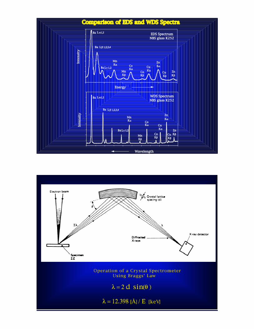
S i ( L i )

Intrinsic

S i l i con

Cut Silicon

Crystal on

Intrinsic Boundaries

Properties of Intrinsic SiliconProperties of Intrinsic Silicon..

Attaching HV electrodes to the two Attaching HV electrodes to the twosurfaces the surfaces the SiSi(Li) crystal will act(Li) crystal will actsimiliar similiar to a capacitor with freeto a capacitor with freecharges developing on the electricalcharges developing on the electricalcontacts. Charge developed in thecontacts. Charge developed in thecrystal is N = E/crystal is N = E/((. (E= x-ray Energy, . (E= x-ray Energy, ((= 3.8 = 3.8 eVeV/e-h pair) i.e. ==> 10 kV X-/e-h pair) i.e. ==> 10 kV X-ray produces ~2630 electrons = 4.2 xray produces ~2630 electrons = 4.2 x10 -16 Coulombs.10 -16 Coulombs.

••P-type Silicon high conductivityP-type Silicon high conductivitydue to impurities (usually Boron);due to impurities (usually Boron);Lithium acts as a compensatingLithium acts as a compensatingdopant dopant neutralizing the neutralizing the Si Si giving itgiving ita high a high resisitivityresisitivity..

•• Radiation deposits energy in the Radiation deposits energy in theSiSi(Li) lattice & creates free(Li) lattice & creates freeelectron-hole pairs in the crystalelectron-hole pairs in the crystal@ 1 electron-hole pair/3.8 @ 1 electron-hole pair/3.8 eV eV ofofdeposited energy @ 77K.deposited energy @ 77K.

•• Intrinsic Intrinsic semiconducting Sisemiconducting Siallows both electrons & holes toallows both electrons & holes tobecome mobile under applicationbecome mobile under applicationof a potential bias across theof a potential bias across thecrystalcrystal

Environmental Isolation Window (Be, Hydro-Carbon, Windowless)

X-R

ay

s

Dead Layer p-type SS Cryostat Housing

FET

-HV

Intrinsic

(Active)

Zone

LN2

Cold

Finger

Au Electrical Contact Dead Layer n-type

=

x

I o I T I o exp (- ! x )[ µ

!] exp (- µ x )=I o

Solid State Detector ConstructionSolid State Detector Construction

Relative Detection EfficiencyRelative Detection Efficiency

Solid State Detectors: Solid State Detectors: SiSi(Li) or (Li) or Instrinsic Instrinsic (High Purity) (High Purity) GeGeUsing a simple absorption model define the relative detector efficiency Using a simple absorption model define the relative detector efficiency (((E)(E)

by the following procedure:by the following procedure:

5 04 03 02 01 000.0

0.2

0.4

0.6

0.8

1.0

Si Active = 3mmSi Active = 5mm

X-ray Photon Energy (keV)

Rela

tiv

e

Eff

icie

ncy

Detector Parameters

Be Window: 8 MicronsAu Contact: 250 ÅSi Dead Layer: 1000 Å

Calculated Si(Li) Detector Efficiency byActive Layer Thickness & Window Type

400030002000100000.0

0.2

0.4

0.6

0.8

1.0

8 Micron Be1000 Å Pyrolene & AluminiumWindowless

X-Ray Photon Energy (eV)

Rela

tiv

e

Eff

icie

ncy

Detector Window Type

Au Contact Layer 250 ÅSi Dead Layer 1000 ÅSi Active Layer 3 mm

0.00

0.20

0.40

0.60

0.80

1.00

0 200 400 600 800 1000

Rela

tive T

ran

smis

sion

Energy ( eV)

Pyrolene N @1000Å

Diamond-Like C @ 0.4 µm

Aluminium @ 1000Å

B-90,N-9,H-1 @ 0.25 µm

Relative Transmission Efficiency

!(E) = IT

Io = exp( "

i

Window

-(µ(E)# )i*#i*ti )

µ(E)#

= mass absorption coefficient for Energy E; # = density; t = layer thickness

Note the Variation in transmission characteristics by Window Type.Note the Variation in transmission characteristics by Window Type.Not all Not all UltraThin UltraThin Windows are Equivalent!!! For example Detection of NitrogenWindows are Equivalent!!! For example Detection of Nitrogen

using a Diamond window is virtually impossible.using a Diamond window is virtually impossible.

109876543210

0.0

0.2

0.4

0.6

0.8

1.0


Calc

ula

ted

D

ete

cto

r

Eff

icie

ncy

S i ( L i )

HP GeDetector Parameters

Be Window: 0 nmGold Contact: 20 nmSi Dead Layer: 100 nmSi Active Layer: 3 mmGe Dead Layer: 200 nmGe Active Layer: 3 mm

100908070605040302010

0.0

0.2

0.4

0.6

0.8

1.0


Calc

ula

ted

D

ete

cto

r

Eff

icie

ncy

S i ( L i )

HP Ge

Detector Parameters

Be Window: 0 nmGold Contact: 20 nmSi Dead Layer: 100 nmSi Active Layer: 3 mmGe Dead Layer: 200 nmGe Active Layer: 3 mm

Calculated EfficiencyCalculated EfficiencySiSi(Li) and (Li) and HPGeHPGe

Windowless SystemsWindowless Systems

0.00

0.20

0.40

0.60

0.80

1.00

0 2 4 6 8 10

Windowless

XEDS Detector

Beryllium Window

XEDS Detector

Ni L

Energy (keV)

O K

Ni K

No

rma

lize

d I

nte

nsi

ty (

Arb

. U

nit

s)

Windowless Windowless vsvs. Conventional Detectors. Conventional DetectorsComparision Comparision of XEDS measurement on of XEDS measurement on NiONiO

using a Windowless versus Beryllium Window detectorusing a Windowless versus Beryllium Window detector

Note the enhanced detection efficiency below 1 Note the enhanced detection efficiency below 1 keV keV for the WL detector. Bothfor the WL detector. Bothspectra are normalized to unity at the Ni Kspectra are normalized to unity at the Ni K## Line (7.48 Line (7.48 keVkeV))

Windowless Windowless vsvs. Conventional Detectors. Conventional Detectors

K Shell Spectra usingK Shell Spectra usingWindowless DetectorWindowless Detector

Boron -> Silicon Boron -> Silicon

L Shell Spectra UsingL Shell Spectra UsingWindowless DetectorWindowless Detector

Titanium ->ZincTitanium ->Zinc

Note Potential Overlaps withNote Potential Overlaps withK shell LinesK shell Lines

ComparisionComparisionLight ElementLight ElementSpectroscopySpectroscopy

ResolutionResolutionXEDSXEDS

((= 3.8 = 3.8 eV eV (in (in SiSi) / 2.9 ) / 2.9 eV eV (in (in GeGe))F = F = Fano Fano Factor ~ 0.1Factor ~ 0.1E= X-ray EnergyE= X-ray EnergyNoise = Electronic Noise (mainly in the FET)Noise = Electronic Noise (mainly in the FET)

Nominal FWHM Values in Modern Nominal FWHM Values in Modern SiSi(Li) Detectors:(Li) Detectors:

O KO K# # (0.52 (0.52 keVkeV)) == 80 to 100 80 to 100 eVeVMn Mn KK## (5.9 (5.9 keVkeV)) = 140 to 160 = 140 to 160 eVeVMo KMo K# # (17.5 (17.5 keVkeV)) = = 210 to 230 210 to 230 eVeV

0.00

200.00

400.00

600.00

800.00

1000.00

0

Inte

nsit

y

0 .4 0.8 1.2 1.6 2

Energy (keV)

High Noise

Intermediate

None

Resolution will also vary withResolution will also vary withMicrophonic Microphonic & Electronic Noise, and Counting& Electronic Noise, and Counting

Rate!Rate!

WL & UTW detectors are WL & UTW detectors are particuliarly particuliarly sensitive to low energysensitive to low energynoise and noise and microphonicsmicrophonics. Observe the changes in the spectra. Observe the changes in the spectra

140.00

150.00

160.00

170.00

180.00

190.00

Cr

Ka

FW

HM

R

eso

luti

on

(e

V)

0 5 K 10K 15K 20K 25K 30K

Count Rate

100 Kv

200 kV

300 kV

Resolution Loss with Count RateResolution Loss with Count Rate

0.00

20.00

40.00

60.00

80.00

100.00

0 5 1 0 1 5 2 0 2 5 3 0 3 5

Count Rate (Thousands)

Cr/Mo 40 usec

NiO/Be 40 usec

NiO/Be 20 usec

Percen

t D

ead

T

ime

MCA/ADC ConsiderationsDetector Dead Time

Instrumentation: AEM SystemsInstrumentation: AEM Systems

The AEM as a system The AEM as a system Spectral Artifacts in the AEM Spectral Artifacts in the AEM

Uncollimated Uncollimated RadiationRadiationSystems PeaksSystems PeaksArtifacts at High Electron EnergyArtifacts at High Electron Energy

Specimen Contamination & Preparation Specimen Contamination & Preparation Optimizing Experimental Conditions Optimizing Experimental Conditions

2 01 51 050

0

1000

2000

3000

Energy (keV)

Inte

nsi

ty

Specimen

2 01 51 050

0

5000

10000

15000

Inte

nsi

ty

Ni4Mo

Specimen

•Stnd C1/C2

Apertures

Ni L

Mo L

Ni K

Mo KFe K

e-

Ni4Mo

Hole Count

•Stnd C1/C2

Apertures

Spectral Artifacts in the AEMUncollimated Radiation: The Hole Count

Variable

Second Condensor

Aperture

Fixed

First Condensor

Aperture

Specimen

and

Goniometer Stage

Upper Objective Pole Piece

Objective Aperture

Lower Objective Pole Piece

X-rays

Electrons

Thick Varia b l e

Second Cond e n s o r

A p e r t u r e

Thick Fixed

First Condensor

A p e r t u r e

Specimen

and

Goniometer Stage


Objective Aperture


Non-Beam De f i n i n g

C o l l i m a t o r

X-rays

Electrons

Spectral Artifacts in the AEMSpectral Artifacts in the AEMUncollimated Uncollimated Radiation SolutionsRadiation Solutions

Variable

Second Condensor

Aperture

Fixed

First Condensor

Aperture

Specimen

and

Goniometer Stage


Objective Aperture


X-rays

Electrons

Mo StndPt Stnd

Au Thin

100 µ m C2 Aperture

Au

Mo, Pt

7654321

10 1

10 2

10 3

10 4

10 5

10 6

Spot Size / C1 Lens Setting

Hole

Cou

nt/

Sp

ecim

en

In

ten

sity

Rati

o p

er

nA

of

Pro

be C

urr

en

t

Uncollimated Uncollimated Radiation: The Hole CountRadiation: The Hole CountEffects of Thickness & Composition of Variable C2 ApertureEffects of Thickness & Composition of Variable C2 Aperture

1 01. 1.01.001

10 1

10 2

10 3

10 4

10 5

10 6

10 7

Probe Current (nA)

Hole

Cou

nt/

Sp

ecim

en

In

ten

sity

Rati

o

per

nA

of

Pro

be C

urr

en

t

50 µm Pt Stnd

150 µ m Pt Stnd 50 µ m Pt Thick

150 µ m Pt Thick

C2 Aperture Thickness

Stnd

Thick

Specimen: 200 Specimen: 200 ÅÅ Molybdenum Film on Holey Carbon supported on a Molybdenum Film on Holey Carbon supported on aStnd Stnd Mo Aperture with 200 Mo Aperture with 200 µµm hole. m hole. ExptExpt. Conditions: 120 kV, Specimen. Conditions: 120 kV, Specimentilted toward tilted toward SiSi(Li) 35 degrees.(Li) 35 degrees.

Spectral Artifacts in the AEMSpectral Artifacts in the AEM

Specimen

Ni4Mo

Specimen

•Thick C1/C2

Apertures

Ni4Mo

Hole Count

•Thick C1/C2

Apertures

Ni L

Mo L

Ni K

Mo KFe K

e-

2 01 51 050

0

5000

10000

15000

Inte

nsi

ty

2 01 51 050

0

500

1000

Energy (keV)

Inte

nsi

ty

Spectral Artifacts in the AEMSpectral Artifacts in the AEM

Specimen

Ni4Mo

Specimen

•Thick C1/C2

Apertures

•Non-Beam

Defining

Aperture

Ni L

Mo L

Ni K

Mo KFe K

e-

2 01 51 050

0

5000

10000

15000

Inte

nsi

ty

2 01 51 050

0

100

200

300

Energy (keV)

Inte

nsi

ty

Ni4Mo

Hole Count

•Thick C1/C2

Apertures

•Non-Beam

Defining

Aperture

Ni4Mo

Specimen

•Thick C1/C2

Apertures

•Non-Beam

Defining

Aperture

Ni L

Mo L

Ni K

Mo KFe K

Hole Count Effects: Modified CHole Count Effects: Modified C11 and C and C22 & &Non-Beam Defining AperturesNon-Beam Defining Apertures

Hole Count Effects: Modified CHole Count Effects: Modified C11 and andCC22 Apertures Apertures

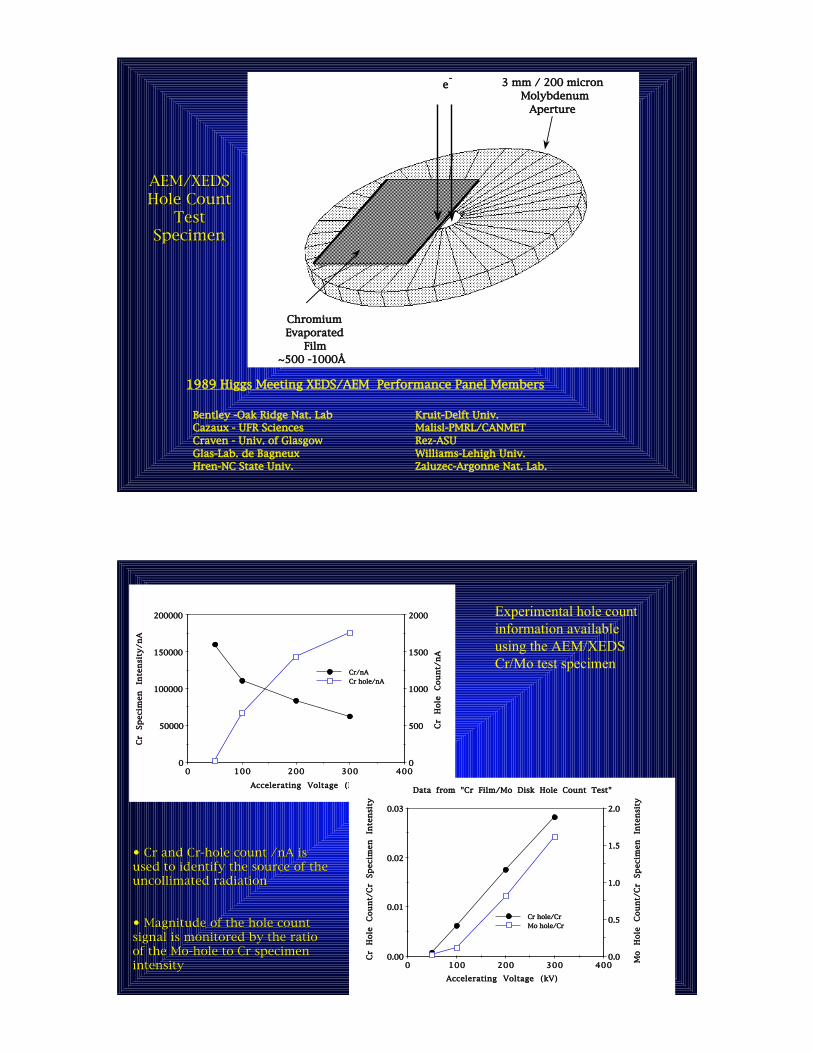
3 mm / 200 micron Molybdenum

Aperture

ChromiumEvaporated

Film~500 -1000Å

e-

Bentley -Oak Ridge Nat. Lab

Cazaux - UFR Sciences

Craven - Univ. of Glasgow

Glas-Lab. de Bagneux

Hren-NC State Univ.

Kruit-Delft Univ.

Malisl-PMRL/CANMET

Rez-ASU

Williams-Lehigh Univ.

Zaluzec-Argonne Nat. Lab.

1989 Higgs Meeting XEDS/AEM Performance Panel Members

AEM/XEDSAEM/XEDSHole CountHole Count

TestTestSpecimenSpecimen

40030020010000

50000

100000

150000

200000

0

500

1000

1500

2000

Cr/nA

Cr hole/nA

Accelerating Voltage (kV)

Cr

Sp

ecim

en

In

ten

sit

y/n

A

Cr

Ho

le

Co

un

t/n

A

40030020010000.00

0.01

0.02

0.03

0.0

0.5

1.0

1.5

2.0

Cr hole/Cr

Mo hole/Cr

Data from "Cr Film/Mo Disk Hole Count Test"


Cr

Ho

le

Co

un

t/C

r

Sp

ecim

en

In

ten

sit

y

Mo

H

ole

C

ou

nt/

Cr

Sp

ecim

en

In

ten

sit

y

•• Cr and Cr-hole count / Cr and Cr-hole count /nA nA isisused to identify the source of theused to identify the source of theuncollimated uncollimated radiationradiation

•• Magnitude of the hole count Magnitude of the hole countsignal is monitored by the ratiosignal is monitored by the ratioof the Mo-hole to Cr specimenof the Mo-hole to Cr specimenintensityintensity

Experimental hole count

information available

using the AEM/XEDS

Cr/Mo test specimen

0

200

400

600

800

1000

0.0 2.0 4.0 6.0 8.0 10.0

Energy (keV)

Low Mag Mode vs. Mag Mode

LM Mode 1.1kX

Mag Mode 1.5kX

Spectral Artifacts in the AEM:Spectral Artifacts in the AEM:Electrons Entering theElectrons Entering the

DetectorDetector50 kV50 kV

0

400

800

1200

1600

2000

0.0 10.0 20.0 30.0 40.0 50.0

Energy (keV)

Low Mag Mode vs. Mag Mode

60.0

LM Mode 1.1kX

Mag Mode 1.5kX

Note the Effects of 50 Note the Effects of 50 keVkeVElectrons Entering the DetectorElectrons Entering the Detectoron Backgroundon Background

1

10

100

1000

10000

100000

0.0 4.0 8.0 12.0 16.0 20.0

LM Mode 1.1kX

Mag Mode 1.5 kX

Energy (keV)

Low Mag Mode vs. Mag Mode300 kV Operation

1

10

100

1000

0.0 10.0 20.0 30.0 40.0 50.0 60.0 70.0 80.0

LM Mode 1.1kX

Mag Mode 1.5 kX

Energy (keV)

Low Mag Mode vs. Mag Mode300 kV Operation

Note the Effects of 300 Note the Effects of 300 keVkeVElectrons Entering theElectrons Entering theDetector on BackgroundDetector on Background

Spectral Artifacts in the AEM:Spectral Artifacts in the AEM:Electrons Entering theElectrons Entering the

DetectorDetector300 kV300 kV

Choice of X-ray Line Choice of X-ray Line K- series K- series L- series L- series M- series M- series

Detector/Specimen Geometry Detector/Specimen Geometry Elevation Angle Elevation Angle Solid Angle Solid Angle

Detector Collimation Detector Collimation

Choice of Accelerating Voltage Choice of Accelerating Voltage Relative Intensity Relative Intensity Peak/ Background Peak/ Background Systems Peaks/ Systems Peaks/Uncollimated Uncollimated RadiationRadiation

Choice of Electron Source Choice of Electron Source Spatial ResolutionSpatial Resolution Tungsten Hairpin Tungsten Hairpin LaB LaB66

Field Emission Field Emission

Optimizing Experimental ConditionsOptimizing Experimental Conditions

! E

e-

SpecimenEucentric

Height

Detector/Specimen Geometry

DesignationDesignation Elevation Elevation Azimuthal Azimuthal ManufacturerManufacturerAngleAngle AngleAngle))EE ))AA

LowLow 00oo 4545oo JEOLJEOL00oo 9090oo JEOL, FEI, VGJEOL, FEI, VG

IntermediateIntermediate 15-3015-30oo 9090oo FEI, JEOL,FEI, JEOL,Hitachi,VGHitachi,VG

HighHigh 68-7268-72oo 00oo Hitachi, JEOLHitachi, JEOL

XEDS

Collimator

CharacteristicX-ray Emission

Angular Dependance(Isotropic Distribution)

Bremsstrahlung Angular Dependance

(Aniostropic Distribution)

High Energy

Low Energy

!

e-


Characteristic

~Isotropic

Continuum

Highly Anisotropic

Collection Solid AngleCollection Solid Angle

* * = A/R= A/R22 = = 0.3 - 0.001 0.3 - 0.001 sRsR AA = Detector Active Area = Detector Active Area

= 10-30 mm2 = 10-30 mm2 R R = Crystal to Specimen Distance = Crystal to Specimen Distance

= 10 - 50 mm = 10 - 50 mm


Subtending Solid Angle

Detection of System Peaks Effects of the Collimator & Stage

Subtending Solid Angle

Removal of Stage System Peaks by use of Beryllium GimbalsRemoval of Stage System Peaks by use of Beryllium GimbalsGe Ge specimen 10,000 in specimen 10,000 in Ge Ge KK# # peak in both spectrapeak in both spectra

Left Standard Single Tilt Cu Stage, Right Be Left Standard Single Tilt Cu Stage, Right Be Gimbal Gimbal DT StageDT Stage

Detection & Removal of System PeaksDetection & Removal of System Peaks

Example:Example:

•• The figure at the right shows the results ofThe figure at the right shows the results of

contamination formed when a 300 kVcontamination formed when a 300 kV

probe isprobe is focussed focussed on the surface of aon the surface of a

freshlyfreshly electropolished electropolished 304 SS TEM304 SS TEM

specimen.specimen.

•• The dark deposits mainly consist ofThe dark deposits mainly consist of

hydrocarbons which diffuse across thehydrocarbons which diffuse across the

surface of the specimen to the immediatesurface of the specimen to the immediate

vicinity of the electron probe. The amountvicinity of the electron probe. The amount

of the contamination is a function of theof the contamination is a function of the

time spent at each location. Here the timetime spent at each location. Here the time

was varied from 15 - 300 seconds.was varied from 15 - 300 seconds.

Reactive Gas Plasma ProcessingReactive Gas Plasma Processing

Applications to Analytical Electron Microscopy Applications to Analytical Electron Microscopy

15 sec15 sec

30 sec 30 sec

60 sec 60 sec

120 sec 120 sec

300 sec 300 sec

44

••After 5 minutesAfter 5 minutesArgon ProcessingArgon Processing

••After 5 minutes ofAfter 5 minutes ofadditional Oxygenadditional OxygenProcessingProcessing

Comparision Comparision Results onResults on Electropolished Electropolished 304 SS304 SS

••UntreatedUntreatedSpecimenSpecimen

99

X-ray Production = Cross-section * electronsX-ray Production = Cross-section * electronsMaximizingMaximizing

The SignalThe Signal

10008006004002000

103

104

105

106

107

Al

Ni

Ag

Voltage (kV)

Rela

tiv

e

Nu

mb

er

of

K-s

hell

Io

niz

ati

on

s

Relativistic Model

Effects on Intensity with Accelerating VoltageEffects on Intensity with Accelerating Voltagefor constant Probe size parametersfor constant Probe size parameters

I = Q * I = Q * && For identical probe diameters one has higher x-ray production at higher For identical probe diameters one has higher x-ray production at higher

voltage due to the increase in beam current.voltage due to the increase in beam current. Alternatively, one can achieve the same statistical intensity for smaller Alternatively, one can achieve the same statistical intensity for smaller

probes at higherprobes at higher

40030020010000.00

0.05

0.10

0.15

0.20

0.25

0

5000

10000

15000

20000Beam Current

Al Ka


Al

Ka

X-r

ay

In

ten

sit

y

Beam

C

urren

t (n

A)

Experimental Variation ofExperimental Variation ofBeam Current and X-ray Intensity with VoltageBeam Current and X-ray Intensity with Voltage

40030020010000

10000

20000

30000

40000

50000

0.00

0.05

0.10

0.15

0.20

0.25Ni Specimen

Beam Current (nA)


Ni

Ka

X-r

ay

In

ten

sit

y

Beam

C

urren

t (n

A)

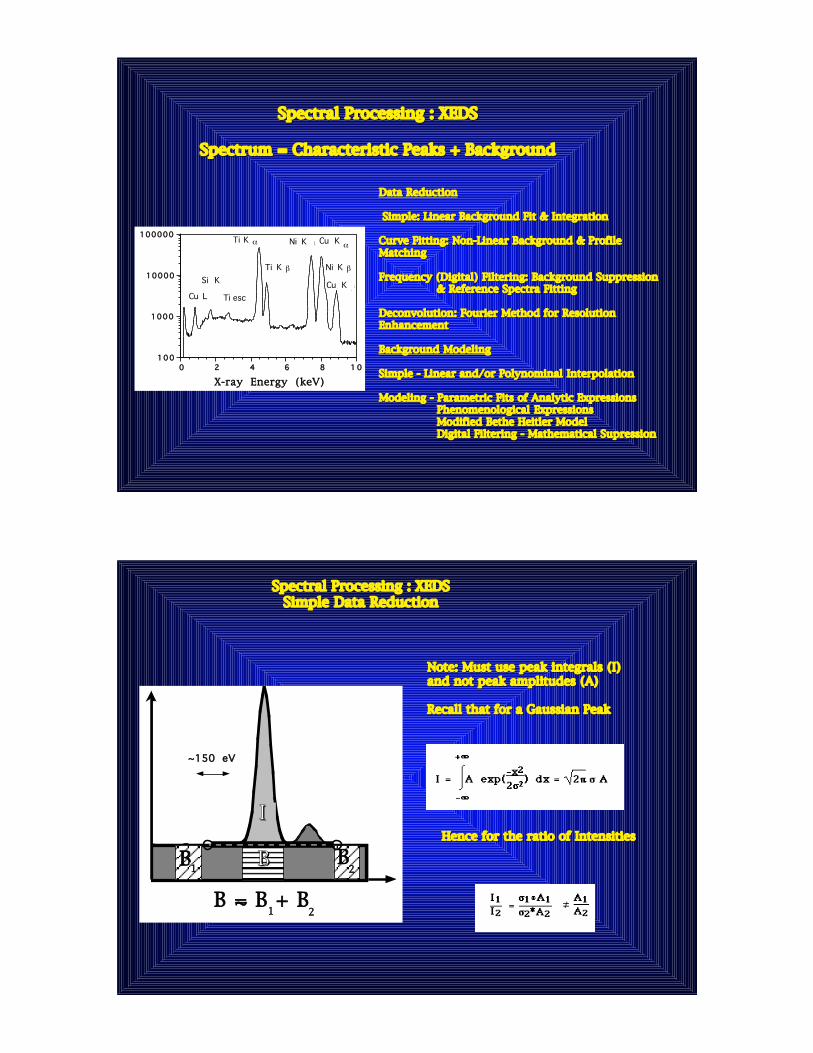
k,kk,k** = Constants = Constants

PPxx = Characteristic Signal= Characteristic Signal from element X from element X

(P/B)(P/B)xx = Peak to Background ratio for element X = Peak to Background ratio for element X

IIo o = Incident electron flux= Incident electron flux

JJoo = Incident electron current density = Incident electron current density

ddo o = Probe diameter= Probe diameter

TT = Analysis time = Analysis time

40030020010000

102030405060708090

100110120

Al P/B 400ÅAl P/B 1200ÅAl P/B 3000Å

Accelerating Voltage (kV) Alu

min

ium

Peak

/B

ack

gro

un

d

Rati

o

ExperimentalExperimental

Peak/BackgroundPeak/Background

Variation with VoltageVariation with Voltage

GoldAluminium

100 kV

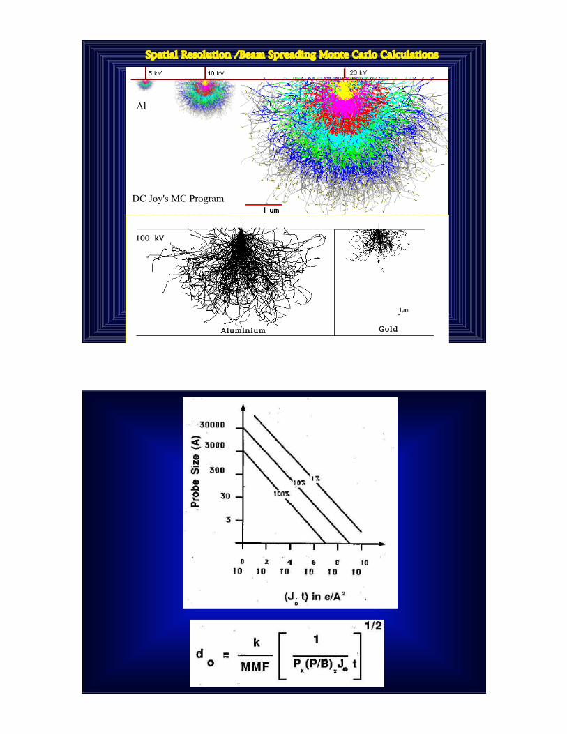
Spatial Resolution /Beam Spreading Monte Carlo CalculationsSpatial Resolution /Beam Spreading Monte Carlo Calculations

DC Joy's MC Program

Al

20

00

Å

100 kV 400 kV 100 kV 400kV

500 ÅA l A l A u A u

Monte Carlo Calculations of Monte Carlo Calculations of BB (Newbury & (Newbury & Myklebust Myklebust -1979)-1979)

ThicknessThicknessElementElement ZZ 10nm10nm 50nm50nm 100nm100nm 500nm500nm

Carbon Carbon 66 0.220.22 1.91.9 4.14.1 33.033.0Aluminium Aluminium 1313 0.410.41 3.03.0 7.67.6 66.466.4Copper Copper 2929 0.780.78 5.85.8 17.517.5 244.0244.0Gold Gold 7979 1.711.71 15.015.0 52.252.2 1725.01725.0

d + B

t

d

ElementElement ZZ 10nm10nm 50nm50nm 100nm100nm 500nm500nmCarbon Carbon 66 0.160.16 1.81.8 5.135.13 57.457.4Aluminium Aluminium 1313 0.260.26 1.91.9 8.128.12 90.990.9Copper Copper 2929 0.680.68 7.67.6 21.421.4 **Gold Gold 7979 15.515.5 17.317.3 ** **

*model invalid at higher kV and/or high scattering angles*model invalid at higher kV and/or high scattering angles

Data Analysis and Quantification:Data Analysis and Quantification:

Spectral Processing Spectral Processing Thin Film Quantification Methods Thin Film Quantification Methods Specimen Thickness Effects: Specimen Thickness Effects:

AbsorptionAbsorptionFluorescenceFluorescence

Ti K ! Ni !K Cu K!

Si K

Ti K " Ni K "

Cu L

"Cu K

Ti esc

1 086420

1 0 0

1000

10000

100000

X-ray Energy (keV)

Inte

nsit

y

(Co

un

ts)

Spectral Processing : XEDSSpectral Processing : XEDS

Spectrum = Characteristic Peaks + BackgroundSpectrum = Characteristic Peaks + Background

Data ReductionData Reduction

Simple: Linear Background Fit & Integration Simple: Linear Background Fit & Integration

Curve Fitting: Non-Linear Background & ProfileCurve Fitting: Non-Linear Background & ProfileMatchingMatching

Frequency (Digital) Filtering: Background SuppressionFrequency (Digital) Filtering: Background Suppression& Reference Spectra Fitting& Reference Spectra Fitting

DeconvolutionDeconvolution: Fourier Method for Resolution: Fourier Method for ResolutionEnhancementEnhancement

Background ModelingBackground Modeling

Simple - Linear and/or Simple - Linear and/or Polynominal Polynominal InterpolationInterpolation

Modeling - Parametric Fits of Analytic ExpressionsModeling - Parametric Fits of Analytic ExpressionsPhenomenological ExpressionsPhenomenological ExpressionsModified Modified Bethe Heitler Bethe Heitler ModelModelDigital Filtering - Mathematical Digital Filtering - Mathematical SupressionSupression

~150 eV

II

B = B + B 1 2

~

B2

B1

BB

Note: Must use peak integrals (I)Note: Must use peak integrals (I)and not peak amplitudes (A)and not peak amplitudes (A)

Recall that for a Gaussian PeakRecall that for a Gaussian Peak

Hence for the ratio of IntensitiesHence for the ratio of Intensities

Spectral Processing : XEDSSpectral Processing : XEDSSimple Data ReductionSimple Data Reduction

Spectral Processing :Spectral Processing :XEDSXEDS

Background Modeling :Background Modeling :Power Law/ParametricPower Law/Parametric

FitsFits

Bgnd = !* A E-Eo

E

2

+ B E-Eo

E+ C

Spectral Processing : XEDSSpectral Processing : XEDSDigital FilteringDigital Filtering

Background Suppression by Mathematical modeling Background Suppression by Mathematical modeling- Replace Data by new spectra formed by the- Replace Data by new spectra formed by the following linear operation. following linear operation.

Operator independentOperator independent Introduces severe spectral distortion Introduces severe spectral distortion

-20

0

20

40

60

80

-2

0

2

4

6

8

50403020100

Gau

ssia

n +

Lin

ear

Fu

ncti

on

Dig

ital F

ilte

r

Digitally Filtered

Original Spectrum

0 10 Energy (keV)

T iN i

Cu

A lC u

Spectral Processing : XEDSSpectral Processing : XEDSDigital FilteringDigital Filtering

X-rays

Generated

Fraction of X-rays

which leave Specimen*

= X-rays

Detected

X-rays

EmittedEfficiency

of Collection*Efficiency

of Detection*

X-rays Generated

per Atom

per Electron

Number of

Incident

Electrons

Number of

Atoms* *

1 + Fraction

Generated by

Secondary

Sources

*

Number of "K" Shell

Ionizations

per Atom per Electron

Number of "K" X-rays

per Ionization*

Fraction of Total "K"

X-rays Measured*

X-ray Production

Quantitative Analysis using XEDSQuantitative Analysis using XEDS

For a thin specimenFor a thin specimen

IIAA == Measured x-ray intensity Measured x-ray intensity per unit areaper unit area

++ == KKthth-shell ionization cross-section-shell ionization cross-section** == KKthth-shell fluorescence yield-shell fluorescence yield,, == KKthth-shell -shell radiative radiative partition functionpartition functionWW == Atomic WeightAtomic WeightNNoo == Avagodro's Avagodro's numbernumber-- == DensityDensityCC == Composition (At %)Composition (At %)&&oo == Incident electron fluxIncident electron fluxtt = = Specimen thicknessSpecimen thickness(( == Detector efficiencyDetector efficiency.. == Detector solid angleDetector solid angle

Ionization Cross-SectionIonization Cross-Section

X-ray Fluorescence Yield has Systematic Variation With Atomic Number

* K shell * K vs * L shell

Quantitative Analysis using XEDSStandardless Method

Invoke the Intensity Ratio Method, that is consider the ratio of x-ray linesfrom two

This simple equation states that the relative intensity ratio of any two

characteristic x-ray lines is directly proportional to the relative

composition ratio of their elemental components multiplied by some

"constants" and is independent of thickness.

NOTE: The kAB factor is not a universal constant!!

Only the ratio of /A//B is a true physical constant and is independant

of the AEM system. The ratio of (A/(B is not a constant since no two

detectors are identical over their entire operational range. This can

cause problems in some cases as we shall see.

The analysis to this point has only yielded the The analysis to this point has only yielded the relative compositionsrelative compositions of the of the

specimen. We need one additional assumption to convert the relative intensityspecimen. We need one additional assumption to convert the relative intensity

ratio's (Iratio's (Iii//IIjj) into ) into compositons compositons namely:namely:

One now has a set of N equations and N unknowns which be solvedOne now has a set of N equations and N unknowns which be solved

algebraically solved for the individual composition values.algebraically solved for the individual composition values.

Thus for a simple two element system we have:Thus for a simple two element system we have:

andand

CCAA + C + CBB = 1. = 1.

oror

Soving Soving for Cfor CBB and C and C

AA

Variation in Measured Composition on 308 SS for Different LabsVariation in Measured Composition on 308 SS for Different Labs

Example in which K-factor is stableExample in which K-factor is stable

Cr, Fe, NiCr, Fe, Ni

Note: Detector efficiency ~ 100% in this energy rangeNote: Detector efficiency ~ 100% in this energy range

Variation in K-factor with AEM/Detector System

Specimen: Uniform NiO film on Be Grid

From: Comparison of UTW/WL X-ray Detectors on TEM/From: Comparison of UTW/WL X-ray Detectors on TEM/STEMs STEMs and and STEMsSTEMs

Thomas, Thomas, CharlotCharlot, , FrantiFranti, , GarrattGarratt-Reed, -Reed, GoodhewGoodhew, Joy, Lee, Ng, , Joy, Lee, Ng, PlictaPlicta, Zaluzec., Zaluzec.

Analytical Electron Microscopy-1984Analytical Electron Microscopy-1984

37.8/62.237.8/62.2 0.74 0.74 9 9

45.8/54.245.8/54.2 1.03 1.03 8 8

47.4/52.647.4/52.6 1.10 1.10 7 7

48.1/51.948.1/51.9 1.13 1.13 6 6

50.4/49.550.4/49.5 1.24 1.24 5 5

50.6/49.450.6/49.4 1.25 1.25 4 4

50.6/49.450.6/49.4 1.25 1.25 3 3

56.1/43.956.1/43.9 1.56 1.56 2 2

80.9/19.180.9/19.1 5.17 5.17 1 1

Apparent VariationApparent Variation

in Compositionin Composition

ExperimentalExperimental

K -Factor K -Factor

InstrumentInstrument

Variation in K-factor with AEM/Detector SystemVariation in K-factor with AEM/Detector System

Low Energy End will not be the only problematic areaLow Energy End will not be the only problematic area

Determining the kAB-1 Factor

Experimental Measurements

Prepare thin-film standards of known composition

then measure relative intensities and solve explicitly

for the kAB factor needed. Prepare a working data base.

This is the "best" method, but

- specimen composition must be verified independently

- must have a standard for every element to be studied

Theoretical Calculations

Attempt first principles calculation knowing

some fundamental parameters of the AEM system

Start with a limited number of kAB factor measurements,

then fit the AEM parameters to best match the data.

Extrapolate to systems where measurements and/or

standards do not exist.

- Method 1. (Goldstein etal) Assume values for ,,*,( and determine the best s to fit kAB. This

procedure essentially iterates the fit of s to the data.

Method 2. (Zaluzec) Assume values for ,,*,+ determine the best e to fit kAB. This

procedure essentially iterates the fit of e (detector window parameters) to the data.

K-Factor Calculation

Experiment

vs

Theory

Sources of values for Sources of values for kkAB AB CalculationsCalculations

WW - International Tables of Atomic Weights- International Tables of Atomic Weights

,,(K)(K) - Schreiber and - Schreiber and Wims Wims , X-ray Spectroscopy (1982), X-ray Spectroscopy (1982)

Vol Vol 11, p. 4211, p. 42

,,(L)(L) - - ScofieldScofield, Atomic and Nuclear Data Tables (1974), Atomic and Nuclear Data Tables (1974)

Vol Vol 14, #2, p. 12114, #2, p. 121

** (K) - (K) - Bambynek etalBambynek etal, Rev. Mod. Physics, , Rev. Mod. Physics, Vol Vol 44, p. 71644, p. 716

Freund, X-ray Spectrometry, (1975) Freund, X-ray Spectrometry, (1975) Vol Vol 4, p.904, p.90

**(L) (L) - Krause, J. Phys. - Krause, J. Phys. ChemChem. Ref. Data (1974) . Ref. Data (1974) Vol Vol 8, 8,

p.307 p.307

++((EoEo)) - - InokutiInokuti, Rev. Mod. Physics, , Rev. Mod. Physics, 4343, , No. 3, 297 (1971)No. 3, 297 (1971)

- Goldstein - Goldstein etaletal, SEM , SEM 11, 315, (1977), 315, (1977)

- Chapman - Chapman etaletal, X-ray Spectrometry, , X-ray Spectrometry, 1212,153,(1983),153,(1983)

- - RezRez, X-ray Spectrometry, , X-ray Spectrometry, 1313, , 55, (1984)55, (1984)

- - EgertonEgerton, , UltramicroscopyUltramicroscopy, , 44, 169, (1969), 169, (1969)

- Zaluzec, AEM-1984, San Fran. Press. 279, (1984)- Zaluzec, AEM-1984, San Fran. Press. 279, (1984)

(( (E) (E) - Use mass absorption coefficients from:- Use mass absorption coefficients from:

--Thinh Thinh and and LerouxLeroux; X-ray ; X-ray SpectSpect. (1979), . (1979), 8,8, p. 963 p. 963

-Henke and -Henke and EbsiuEbsiu, Adv. in X-ray Analysis,, Adv. in X-ray Analysis,17,17, (1974) (1974)

-Holton and Zaluzec, AEM-1984, San Fran Press,353,(1984)-Holton and Zaluzec, AEM-1984, San Fran Press,353,(1984)

Invoke the Intensity Ratio Method, but now consider the ratio of theInvoke the Intensity Ratio Method, but now consider the ratio of the

same x-ray line from two different specimens, where one is from asame x-ray line from two different specimens, where one is from a

standardstandard of known composition while the other is of known composition while the other is unknownunknown::

Quantitative Analysis using XEDSQuantitative Analysis using XEDSThin Film Standards MethodThin Film Standards Method

This simple equation states that the relative intensity ratio of sameThis simple equation states that the relative intensity ratio of same

characteristic x-ray line is directly proportional to the relativecharacteristic x-ray line is directly proportional to the relative

composition ratio of the two specimens multiplied by a some newcomposition ratio of the two specimens multiplied by a some new

parameters.parameters.

& & = incident beam current= incident beam current

-- = local specimen density = local specimen density

t = local specimen thicknesst = local specimen thickness

Quantitative Analysis using XEDSQuantitative Analysis using XEDSSpecimen Thickness EffectsSpecimen Thickness Effects

For finite thickness specimens, what is a thin film?For finite thickness specimens, what is a thin film?

Previous Assumptions:Previous Assumptions: No Energy loss, No Energy loss, No X-ray absorption, No X-ray absorption, No X-ray fluorescence No X-ray fluorescence

NOTE: NOTE: Electron Transparency is insufficient!Electron Transparency is insufficient!

Effects of energy loss on Characteristic X-ray Production:Effects of energy loss on Characteristic X-ray Production:

Quantitative Analysis using XEDS : Absorption CorrectionQuantitative Analysis using XEDS : Absorption Correction

SpecimenSpecimen Homogenity Homogenity

In this and all other derivations we have assumed that over the excitedIn this and all other derivations we have assumed that over the excitedvolume, as well as alongvolume, as well as along th th exitingexiting pathlength pathlength, the specimen is homogeneous in, the specimen is homogeneous incomposition. If this assumption is invalid, one must reformulate thecomposition. If this assumption is invalid, one must reformulate theabsorption correction and take into account changes in : absorption correction and take into account changes in : µ/-, -µ/-, -, and t along the, and t along theexitingexiting pathlength pathlength..

Effects of Beam BroadeningEffects of Beam Broadening

Parallel Slab Model: No Change in absorptionParallel Slab Model: No Change in absorption pathlength pathlengthWedge Model:Wedge Model: There is a correction the magnitude ofThere is a correction the magnitude of

which varies with the wedge angle.which varies with the wedge angle.

Effects of Irregular SurfaceEffects of Irregular Surface

This cannot be analytically modeled but must be understood!This cannot be analytically modeled but must be understood!

X-Ray Fluorescence CorrectionX-Ray Fluorescence Correction

Additional TopicsAdditional Topics

Heterogeneous Specimens Heterogeneous Specimens

Composition Profiles Composition Profiles

Electron Channeling Electron Channeling

Radiation Damage Radiation Damage

Fe Fe

Ni Ni

CrCr

Distance (nm) Distance (nm)-200 -200+200 +200

Grain Boundary Segregation

C*(x,y) = C(x,y,z)* d(x,y,z)

C* (x,y) = Apparent profile measured

C(x,y,z) = Actual composition profile

d(x,y,z) = Incident beam profile

* = Convolution operator

F,F- 1 = Fourier and Inverse Fourier Transforms

In the 2 dimensional limit one can deconvolute themeasured profile using:

C(x,y) = F-1!"#"$

%"&"'F{C*(x,y)}

F{d(x,y)}

Realistically, it is better to decrease the probe diameterand specimen thickness

•• Characteristic X-ray Emission is not trulyCharacteristic X-ray Emission is not truly

isotropic in crystalline materials! isotropic in crystalline materials!

•• Original Observations of EffectOriginal Observations of Effect

–– DuncumbDuncumb ‘‘62, Hall 62, Hall ‘‘66,66, Cherns etal Cherns etal ‘‘7373

•• Predicted ApplicationsPredicted Applications

–– Cowley Cowley ‘‘64, 64, ‘‘7070

•• ACHEMI Technique -ACHEMI Technique -

–– TaftoTafto ‘‘79, Spence &79, Spence & Tafto Tafto ‘‘8383

•• Multi-Multi-VariateVariate Statistical Analysis - Statistical Analysis -

–– Rossouw etalRossouw etal , Anderson and others , Anderson and others

late80late80’’-90-90’’ss

Electron Channeling Induced X-ray EmissionElectron Channeling Induced X-ray Emission

1200

1400

1600

1800

2000

2200

- 2 - 1 0 1 2

AlK

g

0

100

200

300

400

500

600

700

800

-3 -2 -1 0 1 2 3

FeKCrK

NiK

g

180

200

220

240

260

280

300

350

400

450

500

550

-4 -2 0 2 4

AlK-10um NiK-10 um

g

High Angular Resolution Electron Channeling X-ray SpectroscopyHigh Angular Resolution Electron Channeling X-ray SpectroscopyHigh Angular Resolution Electron Channeling X-ray Spectroscopy

0

100

200

300

400

500

600

700

800

-3 -2 -1 0 1 2 3

FeKCrK

NiK

g

2

2.5

3

3.5

4

4.5

5

-3 -2 -1 0 1 2 3

Fe/Cr

Fe/Ni

g

Orientation Dependance in Homogeneous Alloys

Applications in Ordered SystemsApplications in Ordered Systems

1

1.5

2

2.5

3

Compare Ni/AL <110>/<100>

<100>

<110>

NiK

/AlK

In

ten

sit

y R

ati

o

g

ALCHEMIALCHEMIAtom Location byAtom Location by CHanneling CHanneling

EMIssionEMIssionTafto Tafto & Spence - Science 1982& Spence - Science 1982

Introduction to XEDS in the...

Documents

Transcript of Introduction to XEDS in the...