Introduction to non-linear systems - SUPSIpeople.dti.supsi.ch/~smt/courses/nonlinearsystems.pdf ·...

Schweizerische Gesellschaft fur Automatik

Association Suisse pour l’Automatique

Associazione Svizzera di Controllo Automatico

Swiss Society for Automatic Control

Introduction to non-linear systems

-6 -4 -2 0 2 4 6-4

-3

-2

-1

0

1

2

3

4

x*sqrt(c)

xdot

*sqr

t(m

)

Dry fric tion model

Scope Learn characteristics of non-linear systems. Learn the difference

between linear and non-linear systems.

Keywords Operating point dependency, stability, frequency behaviour, limit

cycles, chaos.

Prerequisites LTI systems

Contact Peter Gruber, [email protected]

Version 1.0

Date May 28, 2010

, Introduction to non-linear systems SGA-ASSPA-SSAC

2 Peter Gruber May 28, 2010

Contents

1 Introduction . . . . . . . . . . . . . . . . . . . . . . . . . . . . . . . . 42 Properties of nonlinear systems . . . . . . . . . . . . . . . . . . . . . 6

2.1 Superposition does not hold . . . . . . . . . . . . . . . . . . . 72.2 Commutativity does not apply . . . . . . . . . . . . . . . . . . 72.3 Transfer function methods fail . . . . . . . . . . . . . . . . . . 82.4 Equilibria (local stability) . . . . . . . . . . . . . . . . . . . . 82.5 Limit cycle . . . . . . . . . . . . . . . . . . . . . . . . . . . . 92.6 Chaotic behaviour . . . . . . . . . . . . . . . . . . . . . . . . 132.7 Jump and hysteresis effects in the frequeny response . . . . . . 152.8 Generation of new frequencies for periodic inputs . . . . . . . 152.9 Inversion is not always possible . . . . . . . . . . . . . . . . . 152.10 Finite escape time . . . . . . . . . . . . . . . . . . . . . . . . 15

3 Analysis methods . . . . . . . . . . . . . . . . . . . . . . . . . . . . . 163.1 Stability definition . . . . . . . . . . . . . . . . . . . . . . . . 163.2 Stability analysis tools . . . . . . . . . . . . . . . . . . . . . . 183.3 Robustness . . . . . . . . . . . . . . . . . . . . . . . . . . . . 223.4 Techniques for determination of time-domain solutions . . . . 22

A.1 Examples of non-linear closed-loop systems . . . . . . . . . . . . . . . 25A.2 System with saturation . . . . . . . . . . . . . . . . . . . . . . . . . . 25A.3 Nonlinear closed-loop . . . . . . . . . . . . . . . . . . . . . . . . . . . 25A.4 Hystheresis . . . . . . . . . . . . . . . . . . . . . . . . . . . . . . . . 27A.5 Simulation of Duffing’s equation . . . . . . . . . . . . . . . . . . . . . 27A.6 Dry friction . . . . . . . . . . . . . . . . . . . . . . . . . . . . . . . . 27

May 28, 2010 Peter Gruber 3


1 Introduction

All physical systems exhibit non-linearities and time-varying parameters to somedegree. Linear systems, described by linear differential equations and functions arealways some idealistic description of real physical systems. As many analysis andsynthesis techniques have been developed for linear systems, non-linear systems areoften analyzed and controlled withthe help of linear techniques. In many cases ofsmall non-linearities, satisfactory results can be obtained. In general, however, linearmethods become restrictive in their application and quite often unrealistic. There-fore many methods have been developed for different kinds of non-linear systems.

In this document, non-linear systems are considered which can described byordinary differential equation and algebraic functions. Systems described by partialdifferential equations are not part of this lecture.

The title “Nonlinear systems” includes the followingx words:

• System: Used as term for the plant, process or open loop system as well asfor the feedback control system. The plant or process includes the processdynamics as well as the actuators and sensors needed to realize the control.Actuators and sensor dynamics are sometimes also integrated into the con-troller. In the following, the term process is used for this part of the controlsystem.

• Nonlinear: A system property that applies to the process, the controller andthe overall control system.

This first part gives an overview of combinations of controller and process. Theprocess (including actuator and sensor) is divided into two classes: linear and non-linear ones.

Figure 1.1 shows the block diagram of a closed-loop control system.

yu+

_

r

d

ProcessController Actuator

Sensorym

Figure 1.1: Control loop set up


SGA-ASSPA-SSAC , Introduction to non-linear systems

Based on the classes above there exist six combinations of controller and process.In the following an example will be given for each combination togehter with themain non-linear characteristics as well as with the possible methods for analysis anddesign.

• Case 1: linear plant and linear controller

• Case 2: linear plant and piecewise linear controller

• Case 3: linear plant and non-linear controller

• Case 4: non-linear plant and linear controller

• Case 5: non-linear plant and piecewise linear controller

• Case 6: non-linear plant and non-linear controller

Most non-linear systems can be classified in one of the following sets:

• Static non linearities. Elements like saturation, dead zone, rate-limiter,backlash and quantization are often present in electronic, electro-mechanicaland mechanical system.

• Hysteresis. Multi-valued functions y = f(x) exist, if two or more functionvalues y1, y2, . . . exist for the same input variable x. Such functions are alwaysnon-linear and need additionally at least one memory element. This kind ofnon-linearity occurs in magnetic elements, sensors and other systems.

• Non linear differential equation. mathematical description of the systembehavior (e.g. population model, relay control, motion affected by Coulombfriction).

Single-valued functions contain no hysteresis, while multivalued functions containone or several hysteresis. In the Simulink library for discontinuous functions seeFig. 1.2 there exist a number of examples for both types.



Discontinuities

Wrap To Zero

SaturationDynamic

up

u

lo

y

Saturation

Relay

Rate LimiterDynamic

up

u

lo

Rate Limiter

Quantizer

Hit Crossing

Dead ZoneDynamic

up

u

lo

y

Dead Zone

Coulomb &Viscous Friction

Backlash

Figure 1.2: Nonlinear discontinuous function library in Simulink.

2 Properties of nonlinear systems

Nonlinear systems exhibit a much richer dynamic behaviour than linear systems.Nonlinear systems include open loop or closed-loop control systems with either in-ternal external or no inputs. An open loop system with one control input u and onedisturbance input d can be represented by the following equations:

y(n) = f(y(n−1), . . . , y, d, u, t)

or in state-space representation as:{

x = f(x, u, d, t)y = g(x, u, d, t)

where f(.) is a vector of n functions. If the independent variable t is only presentin the input u or d but not in the parameters of the equation, the system is timeinvariant.

A nonlinear time invariant system, described by an ordinary differential equation,can be represented by the input-output block representation of Figure 1.3:

The systems behaviour is primarily determined by the structure of the differ-ential equation and by the nonlinearities involved. The solutions are however alsodependent on the following quantities:

• Initial conditions x(0)



can be represented by the following input output block presentation:

u y

d

),,,....,( )1()( duyyfy nn −=Initial conditionsparameters

Figure 1.3: Nonlinear LTI block diagram.

• Control input u

• Disturbance input d including its time variation and other uncertainties

• Parameters including the time dependency and other uncertainties

Some properties of nonlinear dynamic systems are

• principle of superposition does not hold

• commutativity does not apply

• possible multiple isolated equilibrium points

• properties such as limit-cycle, bifurcation, chaos

• finite escape time: solutions of nonlinear systems may not exist for all times

2.1 Superposition does not hold

The output y(t), t ≥ 0 of a SISO dynamic system with constant parameters dependson two things: the initial conditions of its state x(0) and the control and disturbanceinputs. For a linear dynamic system one can find the general solution for

y(t) = f(t) + g(t) ∗ u(t)

for t ≥ 0 by superposition of the free response f(t) which depends on the initial con-ditions and the forced response g(t)∗u(t) which depends on the input. Unfortunatelythis approach is no longer valid for nonlinear systems because the superposition oraddition of solutions can no more be used. Therefore the impulse or step responsescannot be used for describing a nonlinear system.

2.2 Commutativity does not apply

Another difficulty is that, except for special combinations of nonlinear operations,nonlinear operations are not interchangeable. Even a linear block and a nonlinearoperation cannot be interchanged.



Example 1 Given are two nonlinear operations:y1 = f1(u1) = u2

1 y2 = f2(u2) = sinu2

y21 = f2(f1(u1)) = sin(u21)

y12 = f1(f2(u1)) = (sin(u1))2

y21 6= y12

Example 2 One linear and one nonlinear operation:y1 = Ku1 y2 = f(u2) = sinu2

y21 = f(y1) = sin(Ku1)y12 = Kf(u1) = K sin(u1)y21 6= y12

2.3 Transfer function methods fail

The terms transfer function, poles and zeros loose their meanings as they do notexist for nonlinear systems. Transfer function methods can be exploited for the linearpart of the system if the nonlinearity can be isolated in- and output connected tolinear part of the system.

2.4 Equilibria (local stability)

An equilibrium is a “static trajectory”: the condition when the state variables arenon-changing, i.e. when the state-variable derivative x is 0. Then

f(y, u, d) = 0

A linear system has a unique equilibrium point if the system matrix A associatedwith the differential equation of the system is nonsingular, that means if the char-acteristic equation of the homogeneous equation has no characteristic values withreal parts equal to zero. Any operating point of a linear system can be transformedto the origin without loss of generality. The stability of the linear system is there-fore determined by the stability of the origin and is given by the location of thecharacteristic values of A. Therefore the system behaviour is not operating pointdependent: the stability property is global and can be associated with the system.

A nonlinear system behaviour however is dependent on the local conditions,that means on the operating point, on the initial conditions and on the inputs tothe system. There may exist also more than one equilibrium points with possiblydifferent stability properties (see 2.2.1).

Example 3 Duffing’s equationDuffing’s equation with negative linear spring force and cubic restoring force

x+ kx− x+ x3 = u k > 0

The equilibrium point for u = 0 is x3 = x There are three solutions to thisequation:

x1 = 1 x2 = −1 x3 = 0



The linearization around the first two equilibrium points leads to the linear dif-ferential equation:

△x+ k△x+ 2△x = △uwhich has two poles in the left half plane, while the third equilibrium point leads to

△x+ k△x−△x = △u

which has one pole in the right half plane.

2.5 Limit cycle

A limit cycle is a phenomen of oscillation peculiar to nonlinear systems. The os-cillatory behaviour, unexplainable in terms of linear theory, is characterized by aconstant amplitude and frequency determined by the nonlinear properties of thesystem. Limit cycles differ from linear oscillation (harmonic oscillator) in that theiramplitude of oscillation is independent of initial conditions. For instance, if a systemhas a stable limit cycle, the system tends to fall into this limit cycle, regardless ofthe initial conditions and input (for global region of attraction).

A limit cycle is easily recognized in the phase plane as an isolated closed path.Limit cycles can also exist in nonlinear feedback systems without an external periodicinput. They can be asymptotically stable, stable or unstable.

Example 4 Van der Pol’s EquationThe dynamic system is given by the equation

x+ e(x2 − 1)x+ x = 0 for e > 0

This is an example of an autonomous system exhibiting one stable limit cycle. Inthe (x, x)-plane this limit cycle is a closed orbit. Starting with initial conditions inthe inner region of the limit cycle, the trajectory spirals outward and approaches theperiodic orbit asymptotically from the inside. The damping in this region is positiveas long as x2 < 1.

Starting in the outer region of the phase plane shows a dampened behaviour of thetrajectories approaching the limit cycle asymptotically from the outside. Of interestis the domain of attraction of this limit cycle. This autonomous system has only onestable limit cycle and its domain of attraction is the whole plane. Figure 1.4 showsthe trajectory in the phase plane and Figure 1.5 shows the limit cycle oscillation asa function of time.

Example 5 Dry friction model [1]Dry or Coulomb friction occurs when the surfaces of two solids are in contact andin relative motion without lubrication. The system shown in Fig. 1.6 illustrates dryfriction. A continuous belt is driven by rollers at a constant speed v0. A block ofmass m connected to a fixed support by a spring of stiffness c rests on the belt. Thefrictional force F between the block and the belt depends on the slip velocity v0 − xand is here modeled by a sign function at the origin of value ±F0.



-3 -2 -1 0 1 2 3 4-4

-3

-2

-1

0

1

2

3

4

x

xdot

Van der Pol with e=2

Figure 1.4: Trajectories in the phase plane of the van der Pol equation with e = 2

0 20 40 60 80 100-4

-3

-2

-1

0

1

2

3

4

time

Van der Pol, e=2, x, xdot

xxdot

Figure 1.5: Limit cycle oscillation of van der Pol’s equation as a function of time

More realistic functions could be modeled easily like combination of Coulomb,viscous or Stribeck friction.

If x is the extension of the spring then the equation of motion is

mx+ cx = F0 · sign(v0 − x)

The term on the right hand side is equal to F0 when v0 > x, and −F0 whenv0 < x. Then the following solutions for the phase paths in these two regions are



m

x

v0

Figure 1.6: Dry friction model

obtained (see Exercise):

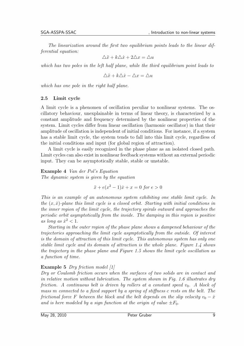
y = x > v0 : my2 + (x+ F0/c)2c = constant

y = x < v0 : my2 + (x− F0/c)2c = constant

These are families of ellipses, the first having its centre at (−F0/c, 0) and thesecond at (F0/c, 0). Fig. 1.7. shows the corresponding phase diagram, plotted as√mx against

√cx to give circular paths. There is a single equilibrium point at

(F0/c, 0), which is of a centre type. On encountering the state x = v0 for |x| < F0/c,the block moves with the belt until the maximum available friction F0 is sufficient toresist the increasing spring tension. This happens when x = F0/c. The block thengoes into an oscillation represented by the closed path through (F0/c, 0). In fact, forany initial conditions lying outside this ellipse, the system ultimately settles into thisoscillation. For frictional forces which are more realistic, the solution paths settle tothe fixed point by a spiral.

Example 6 Population model (Lotka-Volterra)

The population model of Lotka-Volterra models the interaction of two populations:

x1 = ax1 − bx1x2

x2 = −cx2 + dx1x2

The variable x1 represents the prey and x2 the predator. Equilibrium points are at(0, 0) and (c/d, a/b). Figure 1.8 shows limit cycle trajectories.

This system exhibits some pecularities:

• All solutions must be positive by definition

• There are infinitely many limit cycles and there is no attraction region for anyof them. So there are also no transient trajectories possible.



-6 -4 -2 0 2 4 6-4

-3

-2

-1

0

1

2

3

4

x*sqrt(c)

xdot

*sqr

t(m

)

Dry fric tion model

Figure 1.7: Dry friction model m = 1, c = 1, F0 = 2, v0 = 2

0 10 20 30 40 50 600

5

10

15

20

25

prey

pred

ator

Lotka-Volterra population model

Figure 1.8: Lotka-Volterra model a = 2, b = 0.5, c = 2,d = 0.2

• The limit cycles are neither stable nor unstable. They are indifferent and rightat the border line between stable and instable cycles. Any small deviation fromthe limit cycle results in a neighbourhood cycle.

• Linearization around the nonzero equilibrium point will reveal two poles on theimaginary axis. So a small deviation from the equilibrium shows an undampedoscillatory behaviour.

Example 7 Relay-controlA relay controlled system is an example of nonlinear system that shows a limit cyclebehaviour. Figure 1.10 shows the block diagram of a relay control system, Figure 1.9



shows a trajectory of the relay control system as a function of time.

TransportDelay

Transfer Fcn

3

s+1Step

Scope

RelayAdd

Figure 1.9: Relay control system, first order system with delay

0 5 10 150

0.5

1

1.5

2

2.5

3

Time in sec

set

poin

t, a

ctua

l val

ue, r

elay

out

put

set pointrelayactual value

Figure 1.10: Relay control (hysteresis of -0.5, 0,5) of first order system with delayof 1 sec

This example cannot be displayed in the phase plane due to the delay element.The effect of the hysteresis is that the larger the hysteresis is the larger is the am-plitude and the period of the oscillation.

2.6 Chaotic behaviour

Nonlinear dynamic systems may present even more complicated behavior. Oscillation-like solutions can be such that no particular period can be associated with: theylook like random-like solutions. The solutions are concentrated inside a certain re-gion without approaching a limit cycle. Because of its often peculiar shape and thestrange solution curves, the region is called a strange attractor. Inside the strangeattractor no state is reached twice even after infinite length of time.



For a continuous system to exhibit chaotic behaviour, the following three neces-sary but not sufficient conditions must be fulfilled:

• The system order must be of order 3 or higher. The third dimension can bethe time in the case of a time varying parameter or if the system has a timedependent input. In three dimensions much more complicated solution curvescan exist than for two dimensions.

• The system must be nonlinear and has stable and unstable equilibrium points.This ensures that solution curves are repelled and attracted depending on thetype of equilibrium point the solution curves move around.

• The nonlinearity must be such that there exist a high sensitivity of the solutionwith respect to initial conditions. This ensures that solutions starting veryclose to an existing solution do not remain neighbouring solutions as timegoes on but can move apart to the existing solution.

Example 8 Duffings’equationDuffings’equation with periodic input x+ kx− x+ x3 = A sin(ωt).

This version of the Duffing’s equation has negative linear damping and positivecubic restoring terms. The corresponding autonomous system (A=0) has equilibriumpoints at x = ±1, (stable spirals when 0 < k < 2

√2), and at x = 0 (saddle point).

With increasing amplitude A of the input, the system shows for a given frequency ωan increasingly complex type of limit cycles until, at a certain amplitude (A = 0.5),it becomes chaotic. If the amplitude is further increased, the system behaviour settlesagain to a limit cycle. Figure 1.11 shows the Duffing’s equation states as a functionof time.

0

200

400

600

−1

−0.5

0

0.5

1−1.5

−1

−0.5

0

0.5

1

1.5

time [s]x

v

Figure 1.11: Duffing’s equation k = 1, ω = 1.2, A = 1.



Other examples of chaotic systems are the Lorenz model for the weather dynamicsor Chua’s double scroll family for a nonlinear electronic circuit.[2]

2.7 Jump and hysteresis effects in the frequeny response

This effect shows up in certain nonlinear systems excited by a sinusoidal input. Thefrequency response shows a jump resonance peak with a hysteresis effect for thesesystems.

Example 9 Duffing’s equation with damping (with positive linear spring force andcubic restoring force, and periodic forcing term)x+ kx+ x+ βx3 = A cos(ωt). [1].

2.8 Generation of new frequencies for periodic inputs

Nonlinear system generate new frequencies if excited by a single frequency. Sta-tionary output oscillations in nonlinear systems with a sinusoidal input can containsubharmonics or higher harmonics of the input frequency (see exercise).

Consider a simple saturation with a sinusoidal input of amplitude larger thanthe saturation value: the Fourier transform will show the generation of the oddharmonics of the input signal.

2.9 Inversion is not always possible

For many design principles, regardless whether the control law explicitely exploitsthe inverse of the model, the possibility to invert the plant model is fundamental.Numerous nonlinear functions encountered in practice, however, are not invertible(e.g. saturation).

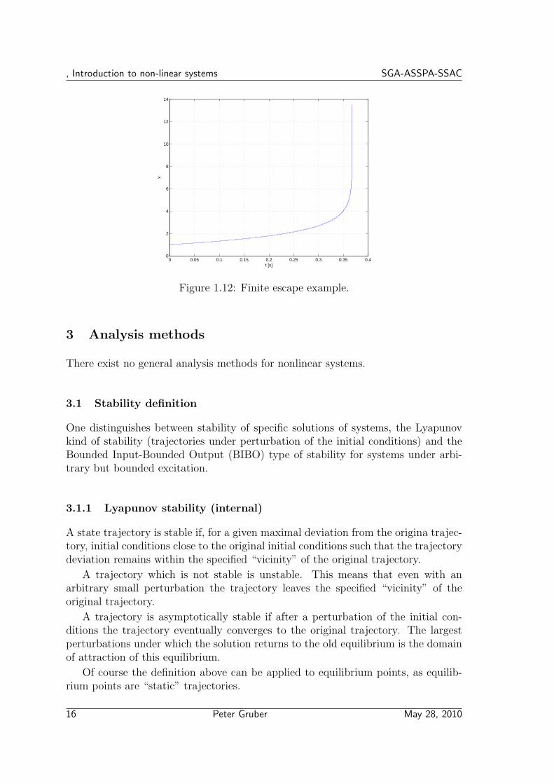
2.10 Finite escape time

The solutions of a nonlinear system may tend to infinity in finite time. Stablenonlinear system for given reference operating points can show this behaviour iflarge over- or undershoots occur due to disturbances. This existence problem innonlinear systems makes the analysis difficult. Various methods for analyzing andsynthesizing nonlinear systems assume that no finite escape time exists.

Example 10 Given is the system

x− ex = 0

with initial condition x(0) = 1. The trajetory is shown in figure 1.12.



0 0.05 0.1 0.15 0.2 0.25 0.3 0.35 0.40

2

4

6

8

10

12

14

t [s]

x

Figure 1.12: Finite escape example.

3 Analysis methods

There exist no general analysis methods for nonlinear systems.

3.1 Stability definition

One distinguishes between stability of specific solutions of systems, the Lyapunovkind of stability (trajectories under perturbation of the initial conditions) and theBounded Input-Bounded Output (BIBO) type of stability for systems under arbi-trary but bounded excitation.

3.1.1 Lyapunov stability (internal)

A state trajectory is stable if, for a given maximal deviation from the origina trajec-tory, initial conditions close to the original initial conditions such that the trajectorydeviation remains within the specified “vicinity” of the original trajectory.

A trajectory which is not stable is unstable. This means that even with anarbitrary small perturbation the trajectory leaves the specified “vicinity” of theoriginal trajectory.

A trajectory is asymptotically stable if after a perturbation of the initial con-ditions the trajectory eventually converges to the original trajectory. The largestperturbations under which the solution returns to the old equilibrium is the domainof attraction of this equilibrium.

Of course the definition above can be applied to equilibrium points, as equilib-rium points are “static” trajectories.



3.1.2 Bounded Input Bounded Output Stability

A system ist BIBO stable, if for zero initial conditions and for any arbitrary butbounded input signal, the output is also a bounded signal. The condition to thesignal is that the power of the input and output signal must be finite. If one thereforefinds one bounded input signal for which the system generates an unbounded outputsignal, the system is proven to be BIBO unstable.

3.1.3 Stability of linear systems

For linear time-invariant systems stability is a global property: for Lyapunov typeof stability, the system is either asymptotically stable, stable or unstable; for BIBOtype of stability either stable or unstable. For linear systems the location of thepoles is responsible for both types of the stability: if they all lie in the left half planethe system is stable. If a pole lies in the right half plane, the system is unstable. Ifone or more poles lie on the imaginary axis and the remaining poles are in the lefthalf plane, the stability issue is more delicate: For the Lyapunov type of stability,the system is stable, for BIBO type of stability the system is unstable.

Example 11 Given is the integrator y(t) =∫ tu(τ)dτ + y(0) with G(s) = 1

s. This

system has a pole at the origin. The equilibrium for zero input is given by the initialcondition y(0) = y

Lyapunov stability: after a change of initial condition: y(0) = y + △y(0) thenew equilibrium is y(t)|t→∞ = y+△y(0) 6= y(0). The system does not return to theold equilibrium, but remains close to it (indifferent equilibrium point). Therefore theintegrator is stable but not asymptotically stable according to Lyapunov.

BIBO stability: Consider the step response u(t) = ǫ(t), then y(t) =∫ tǫ(τ)dτ =

t · ǫ(t). This output to a bounded input is not bounded and therefore the integratoris BIBO unstable.

3.1.4 Stability in nonlinear systems

In nonlinear systems stability is generally a local issue in contrast to linear systems.Different types of equilibrium points may exist. The Lyapunov stability can bedetermined by analyzing the poles of the locally linearized system linearized aroundthe equilibrium point.

If one of the poles (eigenvalue) lies in the right half plane, the equilibrium isunstable, if all poles are in the left half plane, the equilibrium is stable, and if oneor more poles lie on the imaginary axis (and the other in the left half plane), noconclusion about the stability of the equilibrium can be drawn (center manifoldtheorem).

For the determination of BIBO type of stability for nonlinear systems othermethods like passivity analysis and the small gain theorem have to be applied.They base strongly on energy concepts.



3.2 Stability analysis tools

Summing up, different methods can be applied to analyse the stability and perfor-mance of nonlinear systems. These tools will be presented in the sequel.

3.2.1 Linearization around an operating point

This analysis method uses the linearization around an operating point to find alinear approximation for the system. The standard stability techniques developedfor linear systems can be applied to the approximation.

3.2.2 Describing function

The descriptive function methods gives approximated information about the sta-tionary system behaviour, particularly indicatind the presence of oscillations. Themethods assumes that the linear part of the system has a low-pass filter character-istic.

The method exploits the Nyquist plot of the linear part of the system (remember:the Nyquist curve is parametrized in function of the frequency). For the nonlinearpart of the system a second plot related to the nonlinear part of the system andparametrized in function of the potential oscillation amplitude is also shown in theNyquist diagram.

The intersection between the two curves represents the value where the systemshows an oscillation (stable or unstable).

3.2.3 Isocline and gradient method

The isocline method allows obtaining precise graphical information about the stateevolution of an autonomous system of the form

x = f(x) ⇒

dx1

dt= x1 = f1(x1, x2)

dx2

dt= x2 = f2(x1, x2)

(1.1)

This method exploits the fact that the division x2/x1 gives

x2

x1

=dx2

dx1

=f2(x1, x2)

f1(x1, x2)

The system trajectories (evolution of x1 in function of d x2 or viceversa) can befound by solving the differential equation above for various initial conditions or bysimulation.

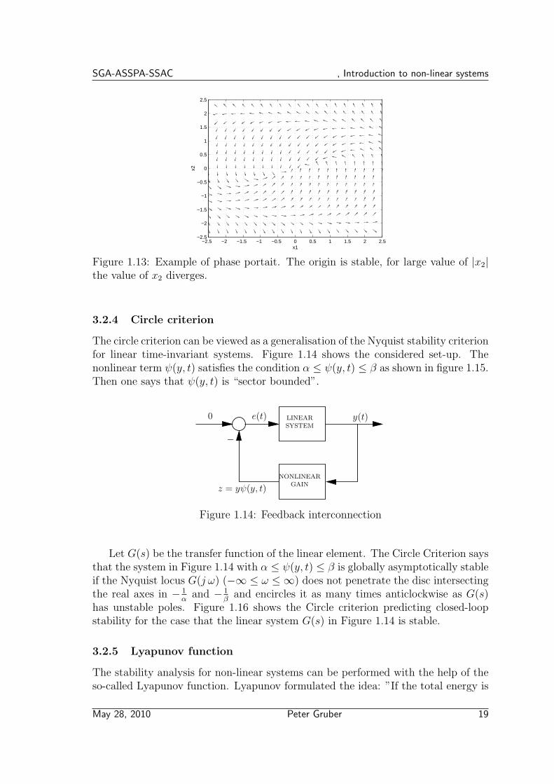
The differential equation obtained above indicates also the trajectory gradientfor each pair (x1, x2). The gradient together with the sense obtained from equation(1.1) can be used to obtain a graphical representation with arrows showing thetrajectory evolution in time. Such a graphical representation, also called “phaseportrait”, is shown in Figure 1.13.



−2.5 −2 −1.5 −1 −0.5 0 0.5 1 1.5 2 2.5−2.5

−2

−1.5

−1

−0.5

0

0.5

1

1.5

2

2.5

x1

x2

Figure 1.13: Example of phase portait. The origin is stable, for large value of |x2|the value of x2 diverges.

3.2.4 Circle criterion

The circle criterion can be viewed as a generalisation of the Nyquist stability criterionfor linear time-invariant systems. Figure 1.14 shows the considered set-up. Thenonlinear term ψ(y, t) satisfies the condition α ≤ ψ(y, t) ≤ β as shown in figure 1.15.Then one says that ψ(y, t) is “sector bounded”.

0

−

e(t) y(t)

z = yψ(y, t)

NONLINEAR

GAIN

LINEAR

SYSTEM

Figure 1.14: Feedback interconnection

Let G(s) be the transfer function of the linear element. The Circle Criterion saysthat the system in Figure 1.14 with α ≤ ψ(y, t) ≤ β is globally asymptotically stableif the Nyquist locus G(j ω) (−∞ ≤ ω ≤ ∞) does not penetrate the disc intersectingthe real axes in − 1

αand − 1

βand encircles it as many times anticlockwise as G(s)

has unstable poles. Figure 1.16 shows the Circle criterion predicting closed-loopstability for the case that the linear system G(s) in Figure 1.14 is stable.

3.2.5 Lyapunov function

The stability analysis for non-linear systems can be performed with the help of theso-called Lyapunov function. Lyapunov formulated the idea: ”If the total energy is



yψ(y, t)

y

Figure 1.15: Sector bounded nonlinearity

G(jω)

−

1

α−

1

βRe

Im

Figure 1.16: Circle criterion proving closed-loop stability for an open-loop stablesystem

dissipated, the system must be stable”.

A Lyapunov function, representing a sort of “energy”, is a positive definite-function, i.e. a function such that

V (0) = 0 and V (x) > 0 ∀x 6= 0



If it can be shown that the time derivative V (x(t)) of this function is decreasing, i.e.

dV (t)

dt< 0

in a certain region around x = 0 then x = 0 is an asymptotically stable equilibriumpoint. If the weaker condition holds that V (x(t)) ≤ 0, the equilibrium is stable.

The stability or asymptotic stability of a system can be determined withoutsolving the nonlinear differential equation. Unfortunately there is no general methodfor the construction of a Lyapunov function for a given system. One can prove thatthe system is stable only if a Lyapunov function is found (by chance or by ability).

The difficulty of solving the differential equation is traded for the problem “Howto find a Lyapunov function?”. The concept of a Lyapunov function can be alsoapplied to time-varying systems and systems with inputs.

Lyapunov functions are in particular commnly used in proving the stability of acontroller for a given system (see more later).

3.2.6 Small gain theorem

In nonlinear systems, the formalism of input-output stability is an important tool instudying the stability of interconnected systems since the gain of a system directlyrelates to how the norm of a signal increases or decreases as it passes throughthe systems. The small-gain theorem gives a sufficient condition for finite-gain Lstability of the feedback connection. The small gain theorem was proved by GeorgeZames in 1966. It can be seen as a generalisation of the Nyquist criterion to non-linear non-time-invariant MIMO systems.

Theorem 1 Assume two systems with MIMO transfer functions S1 and S2 areconnected in a feedback loop; then the closed-loop system is input-output stable if‖S1‖ · ‖S2‖ < 1.

The norm ‖.‖ can be the infinity norm, that is the size of the largest singular valueof the transfer function over all frequencies. Other induced norms can be used [3].

3.2.7 Passivity analysis

A passive system is one that consumes energy. The energy E provided by thesystems with an initial state x0 is defined as

E = supT≥0

∫ T

0

< u, y > dt

∣

∣

∣

∣

x(0)=x0

The supremum is taken over all T ≥ 0 and all admissible pairs (u(), y()) with thefixed initial state x(0) = x0. A system is considered passive if E is finite for allinitial states x(0). Otherwise, the system is considered active. Roughly speaking,the inner product is the instantaneous power, and E is the upper bound on the



integral of the instantaneous power (i.e., energy). This upper bound (taken over allT ≥ 0) is the available energy in the system for the particular initial condition x(0).

Passivity, in most cases, can be used to demonstrate that passive system willbe stable under specific criteria. Passive systems will not necessarily be stableunder all stability criteria. For instance, a resonant series LC circuit will haveunbounded voltage output for a bounded voltage input, but will be stable in the senseof Lyapunov, and given bounded energy input will have bounded energy output.

Passivity is frequently used in control systems to design stable control systemsor to show stability in control systems.

3.3 Robustness

Robustness is treated as in linear systems with respect to the following points:

• Sensitivity with respect to parameter variations of the process (e.g. structuralrobustness, catastrophe theory)

• Sensitivity with respect to initial conditions (e.g. stability of solutions, chaoticbehaviour)

• Sensitivity with respect to control inputs (e.g. jump phenomena, Windup)

• Sensitivity with respect to disturbance inputs (e.g. windup, unknown butbounded uncertainties, stochastic control)

3.4 Techniques for determination of time-domain solutions

For specific differential equations exact solution methods exist like for:

• Equations where the separation of variables is possible.

• Exact differential equations

• Equations with an integrating factor

• First order differential equations in x and t.

• Implicit differential equations where the substitution of variables is possible.

However, no general method for finding solutions are available.


Bibliography

[1] D. W. Jordan and Smith, editors. Nonlinear ordinary differential equation.Clarendon Press Oxford, 1989. Thorough treatment of analysis methods fordynamical system or low order. Medium level.

[2] L.Chua, M. Komuro, and T. Matsumoto. Automatica, 33(11):1072–11182, 1986.

[3] H. K. Khalil, editor. Nonolinear system. Prentice-Hall, 2002. Standard bookin many courses on nonlinear system and control, theoretically oriented.

[4] W. S. Levine, editor. The control handbook. CRC Press, 1996. Very broad forevery aspects of control, covers many methods, differs from author to author inthe theoretical background needed to understand the individual contribution.

[5] D. Bertsekas, editor. Dynamic programming, deterministic and stochastic mod-els. Prentice-Hall, 1987. Together with Dreyfus book on dynamic programmingthe reference book for optimization and control of nonlinear discrete time dy-namical systems with and without uncertainties by the dynamic programmingmethod. Medium to high level.

[6] O. Foellinger, editor. Nichtlineare Regelung I und II. Oldenburg, 1969, 1980.Classic books in german for the analysis and design of nonlinear system viadescribing function method, phase plane methods, Lyapunov function. Veryreadable.

[7] H. Schwarz, editor. Nichtlineare Regelungsysteme. Oldenburg, 1991. Coversfeedback linearization and Volterra series expansion techniques. Voluminous,not easily readable.

[8] K.H. Seitz, editor. Regelung mit Zwei- und Dreipunktregeln. Oldenburg, 1986.Covers many type of discontinuous controller and linear system combinations.Practically oriented.

[9] VDI-Tagung: Nichtlineare Regelung, Methoden, Werkzeuge, Anwendungen.In Bericht, number 1026. VDI Verlag, 1993. Interesting book as it comparesdifferent methods (including fuzzy control) of designing a nonlinear controllerfor three given processes: a mixing tank, an electromechanical actuator an ahydraulic drive.



[10] Anders Robertson. Nonlinear control theory. Technical report, Lund University,2006. Lecture notes, very good summary of important results for nonlinearsystems and control.

[11] Michael D. Lemmon. Nonlinear control. Technical report, Clemson University,South Carolina, 2004. Lecture notes, very good summary of important resultsfor nonlinear systems and control.



Exercises

A.1 Examples of non-linear closed-loop systems

Find examples for the different controller-plant combinations of section 1

A.2 System with saturation

Study the behaviour of the following system consisting of an integrator followed bya limiter if it is excited by a sinusoidal function (see figure 1.17) The amplitude andthe frequency of the input, the initial condition of the integrator and the height ofthe limiting function are parameters. Show the difference between the linear andthe nonlinear case (no limiter).

Sine Wave Scope2Saturation

1s

Integrator2

Figure 1.17: System with saturation

A.3 Nonlinear closed-loop

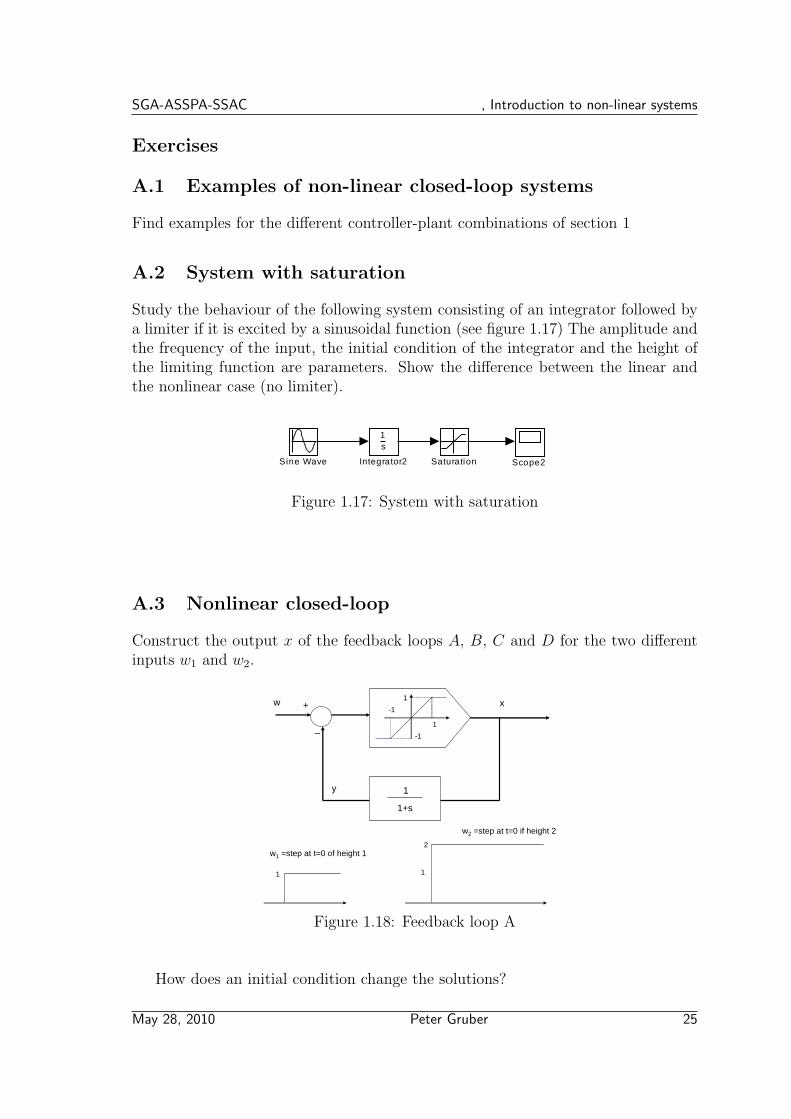
Construct the output x of the feedback loops A, B, C and D for the two differentinputs w1 and w2.

1

1+s

+

_

xw

y

1

1

-1

-1

1

w1 =step at t=0 of height 1

1

w2 =step at t=0 if height 2

2

Figure 1.18: Feedback loop A

How does an initial condition change the solutions?



1

1+s

+

_

xw

y

-1

1

1-1

1


1


2

Figure 1.19: Feedback loop B

1

s

+

_

xw

y

1

1

-1

-1

1


1

2

Figure 1.20: Feedback loop C

1

s

+

_

xw

y

-1

1

1-1

1


1


2

Figure 1.21: Feedback loop D



A.4 Hystheresis

Why is a hysteresis always a nonlinear element?

A.5 Simulation of Duffing’s equation

Simulate the following nonlinear equation (Duffing’s equation) with periodic input:

x+ kx+ x+ βx3 = A sin(ωt)

with k = 0.005, β = 0.2, A = 0.05 and ω = 1. What output frequencies do occur?Try out other amplitudes A and frequencies ω.

A.6 Dry friction

Show that for the dry friction model the phase paths are ellipses.


Introduction to non-linear systems - SUPSIpeople.dti.supsi.ch/~smt/courses/nonlinearsystems.pdf ·...

Documents

Transcript of Introduction to non-linear systems - SUPSIpeople.dti.supsi.ch/~smt/courses/nonlinearsystems.pdf ·...