Introduction to Multilevel Models for Longitudinal Data · Introduction to Multilevel Models for...

Introduction to Multilevel Models for Longitudinal Data

Lecture 1 1

• Topics: What is multilevel modeling? Concepts in longitudinal data From between-person to within-person models Introduction to multilevel modeling via software Kinds of ANOVAs for longitudinal data

What is a Multilevel Model (MLM)?• Same as other terms you have heard of: General Linear Mixed Model (if you are from statistics)

Mixed = Fixed and Random effects Random Coefficients Model (also if you are from statistics)

Random coefficients = Random effects = latent variables/factors Hierarchical Linear Model (if you are from education)

Not the same as hierarchical regression

• Special cases of MLM: Random Effects ANOVA or Repeated Measures ANOVA (Latent) Growth Curve Model (where “Latent” implies SEM) Within-Person Fluctuation Model (e.g., for daily diary data) Clustered/Nested Observations Model (e.g., for kids in schools) Cross-Classified Models (e.g., “value-added” models) Psychometric Models (e.g., factor analysis, item response theory)

Lecture 1 2

The Two Sides of Any Model• Model for the Means: Aka Fixed Effects, Structural Part of Model What you are used to caring about for testing hypotheses How the expected outcome for a given observation varies as a

function of values on predictor variables

• Model for the Variance: Aka Random Effects and Residuals, Stochastic Part of Model What you are used to making assumptions about instead How residuals are distributed and related across observations

(persons, groups, time, etc.) these relationships are called “dependency” and this is the primary way that multilevel models differ from general linear models (e.g., regression)

Lecture 1 3

Review: Variances and Covariances

Lecture 1 4

Variance:Dispersion of y

N = # people, t = time, i = personk = # fixed effects, yti = y predicted from fixed effects

Covariance:How y’s go together, unstandardized

Correlation:How y’s go together, standardized (−1 to 1)

N

2ti ti

i 1t

(y y )Variance (y )

N k

N

1i 2i1i 2ii 1

1 2

(y y )(y y )Covariance (y ,y )

N k

1 21 2

1 2

Covariance(y ,y )Correlation (y ,y )Variance(y ) * Variance(y )

Dimensions for Organizing Models• Outcome type: General (normal) vs. Generalized (not normal)• Dimensions of sampling: One (so one variance term per outcome) vs.

Multiple (so multiple variance terms per outcome) OUR WORLD

• General Linear Models: conditionally normal outcome distribution, fixed effects (identity link; only one dimension of sampling)

• Generalized Linear Models: any conditional outcome distribution, fixed effects through link functions, no random effects (one dimension)

• General Linear Mixed Models: conditionally normal outcome distribution, fixed and random effects (identity link, but multiple sampling dimensions)

• Generalized Linear Mixed Models: any conditional outcome distribution,fixed and random effects through link functions (multiple dimensions) Same concepts as for this week, but with more complexity in estimation

• “Linear” means fixed effects predict the link-transformed conditional mean of DV in a linear combination of (effect*predictor) + (effect*predictor)…

Lecture 1 5

Note: Least Squares is only for GLM

What can MLM do for you?1. Model dependency across observations

• Longitudinal, clustered, and/or cross-classified data? No problem!

• Tailor your model of sources of correlation to your data

2. Include categorical or continuous predictors at any level• Time-varying, person-level, group-level predictors for each variance

• Explore reasons for dependency, don’t just control for dependency

3. Does not require same data structure for each person• Unbalanced or missing data? No problem!

4. You already know how (or you will soon)!• Use SPSS Mixed, SAS Mixed, Stata, Mplus, R, HLM, MlwiN…

• What’s an intercept? What’s a slope? What’s a pile of variance?

Lecture 1 6

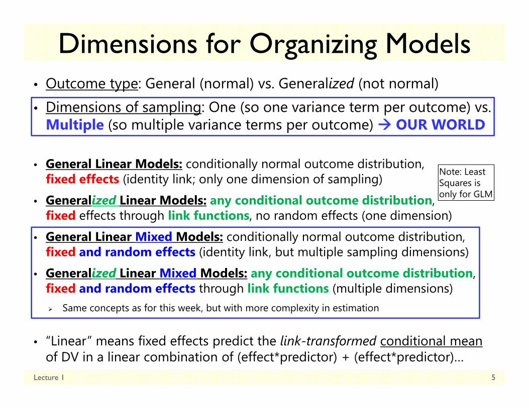
1. Model Dependency• Sources of dependency depend on the sources of

variation created by your sampling design: residuals for outcomes from the same unit are likely to be related, which violates the GLM “independence” assumption

• “Levels” for dependency =“levels of random effects” Sampling dimensions can be nested

e.g., time within person, time within group, trial within person If you can’t figure out the direction of your nesting structure,

odds are good you have a crossed sampling design instead e.g., persons crossed with items, raters crossed with targets

To have a “level”, there must be random outcome variation due to sampling that remains after including the model’s fixed effects e.g., treatment vs. control does not create another level of “group”

(but it would if you had multiple treatment and multiple control groups)

Lecture 1 7

Dependency comes from…• Mean differences across sampling units (persons, groups) Creates constant dependency over time Will be represented by a random intercept in our models

• Individual/group differences in effects of predictors Individual differences in change over time, stress reactivity Group differences in change over time, time-specific effects Creates non-constant dependency, the size of which depends

on the value of the predictor at each occasion or for each person Will be represented by random slopes in our models

• Non-constant within-person correlation for unknown reasons (time-specific autocorrelation) Can add other patterns of correlation as needed for this (AR, TOEP)

Lecture 1 8

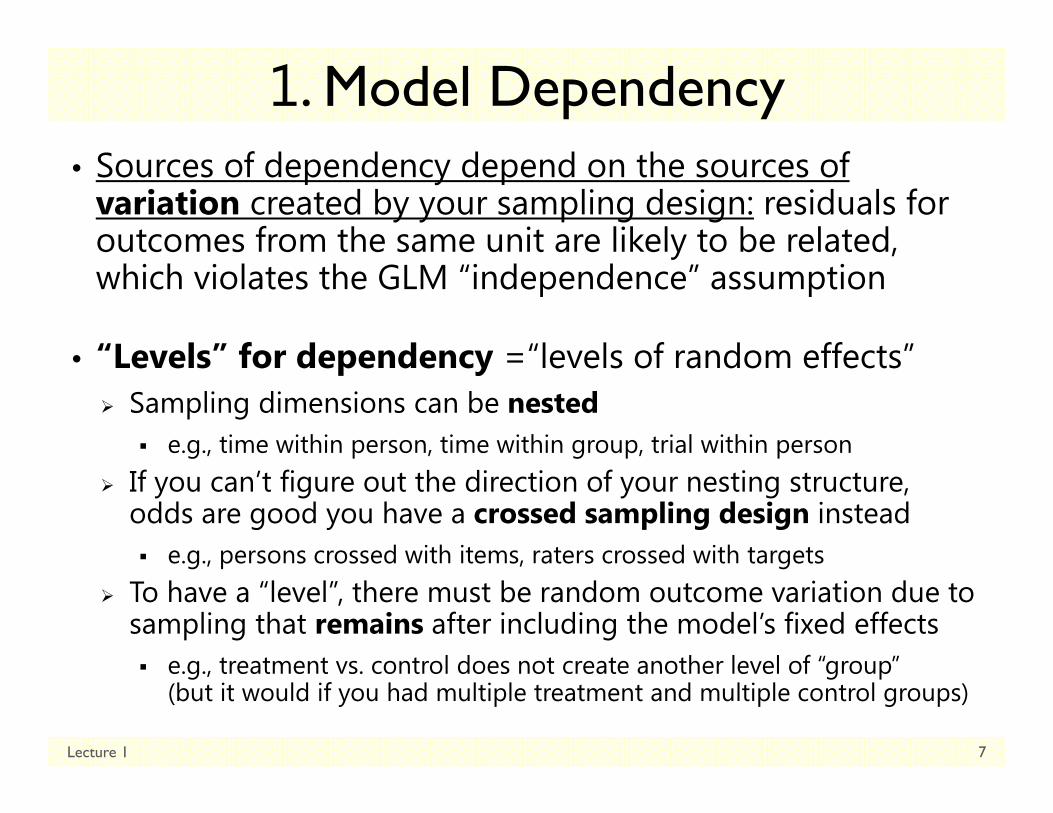
Why care about dependency?• In other words, what happens if we have the wrong model

for the variance (assume independence instead)?

• Validity of the tests of the predictors depends on having the “most right” model for the variance Estimates will usually be ok come from model for the means Standard errors (and thus p-values) can be inaccurate

• The sources of variation that exist in your outcome will dictate what kinds of predictors will be useful Between-Person variation needs Between-Person predictors Within-Person variation needs Within-Person predictors Between-Group variation needs Between-Group predictors Within-Group variation needs Within-Group predictors

Lecture 1 9

2. Include categorical or continuous predictors at any level of analysis

• ANOVA: test differences among discrete IV factor levels Between-Groups: Gender, Intervention Group, Age Groups Within-Subjects (Repeated Measures): Condition, Time Test main effects of continuous covariates (ANCOVA)

• Regression: test whether slopes relating predictors to outcomes are different from 0 Persons measured once, differ categorically or continuously on a

set of time-invariant (person-level) covariates

• What if a predictor is assessed repeatedly (time-varying predictors) but can’t be characterized by “conditions”? ANOVA or Regression won’t work you need MLM

Lecture 1 10

2. Include categorical or continuous predictors at any level of analysis

• Some things don’t change over measurements… Sex, Ethnicity

Time-Invariant Predictor = Person Level

• Some things do change over measurements… Health Status, Stress Levels, Living Arrangements

Time-Varying Predictor = Time Level

• Some predictors might be measured at higher levels Family SES, length of marriage, school size, country size

• Interactions between levels may be included, too Does the effect of health status differ by gender and SES?

Level: Time Person Family

Lecture 1 11

3. Does not require same data structure per person (by accident or by design)

Lecture 1 12

ID Sex Time Y

100 0 1 5

100 0 2 6

100 0 3 8

100 0 4 12

101 1 1 4

101 1 2 7

101 1 3 .

101 1 4 11

MLM: uses stacked (long) data structure:

Only rowsmissing data are excludedID 100 uses 4 casesID 101 uses 3 cases

RM ANOVA: uses multivariate (wide) data structure:

People missing any data are excluded (data from ID 101 are not included at all)

ID Sex T1 T2 T3 T4

100 0 5 6 8 12

101 1 4 7 . 11

Time can also be unbalanced across people such that each person can have his or her own measurement schedule: Time “0.9” “1.4” “3.5” “4.2”…

4. You already know how!• If you can do GLM, you can do MLM

(and if you can do generalized linear models, you can do generalized multilevel models, too)

• How do you interpret an estimate for… the intercept?

the effect of a continuous variable?

the effect of a categorical variable?

a variance component (“pile of variance”)?

Lecture 1 13


Lecture 1 14


Options for Longitudinal Models• Although models and software are separate, longitudinal

data can be analyzed via multiple analytic frameworks: “Multilevel/Mixed Models”

Dependency over time, persons, groups, etc. are modeled via random effects (multivariate univariate through “levels” of stacked/long data)

Builds on GLM, generalizes more easily to additional levels of analysis and crossed dimensions of sampling

“Structural Equation Models” Dependency over time only is modeled via latent variables

(single-level analysis using multivariate/wide data) Generalizes easier to broader analysis of latent constructs, mediation,

and multivariate multilevel models in general (aka, “Multilevel SEM”)

Because random effects and latent variables are the same thing, many longitudinal models can be specified/estimated either way

Lecture 1 15

Data Requirements for Our Models• A useful outcome variable: Has an interval scale*

A one-unit difference means the same thing across all scale points In subscales, each contributing item has an equivalent scale *Other kinds of outcomes can be analyzed using generalized

multilevel models instead, but estimation will be more challenging

Has scores with the same meaning over observations Includes meaning of construct Includes how items relate to the scale Implies measurement invariance

• FANCY MODELS CANNOT SAVE BADLY MEASURED VARIABLES OR CONFOUNDED RESEARCH DESIGNS.

Lecture 1 16

Requirements for Longitudinal Data• Multiple OUTCOMES from the same sampling unit!

2 is the minimum, but just 2 can lead to problems: Only 1 kind of change is observable (1 difference) Can’t distinguish “real” individual differences in change from error Repeated measures ANOVA is just fine for 2 observations

– Necessary assumption of “sphericity” is satisfied with only 2 observations even if compound symmetry doesn’t hold

More data is better (with diminishing returns) More occasions better description of the form of change More persons better estimates of amount of individual differences

in change; better prediction of those individual differences More items/stimuli/groups more power to show effects of

differences between items/stimuli/groups

Lecture 1 17

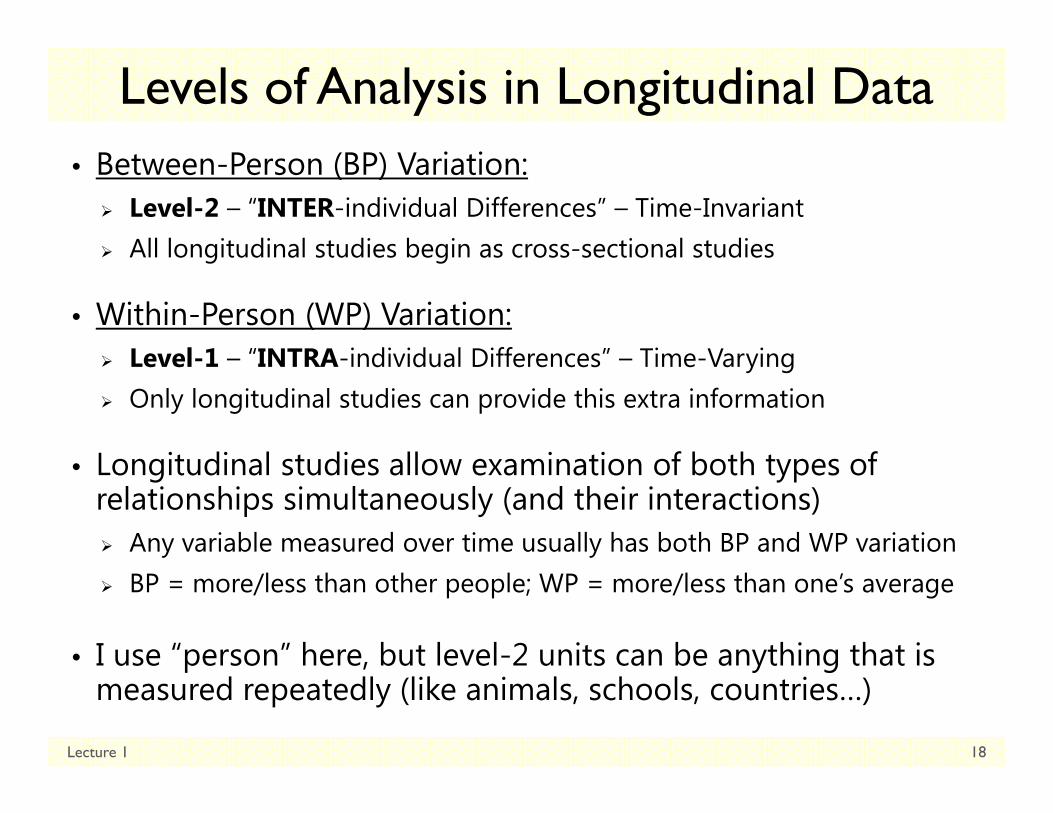
Levels of Analysis in Longitudinal Data• Between-Person (BP) Variation:

Level-2 – “INTER-individual Differences” – Time-Invariant All longitudinal studies begin as cross-sectional studies

• Within-Person (WP) Variation: Level-1 – “INTRA-individual Differences” – Time-Varying Only longitudinal studies can provide this extra information

• Longitudinal studies allow examination of both types of relationships simultaneously (and their interactions) Any variable measured over time usually has both BP and WP variation BP = more/less than other people; WP = more/less than one’s average

• I use “person” here, but level-2 units can be anything that is measured repeatedly (like animals, schools, countries…)

Lecture 1 18

A Longitudinal Data Continuum• Within-Person Change: Systematic change

Magnitude or direction of change can be different across individuals “Growth curve models” Time is meaningfully sampled

• Within-Person Fluctuation: No systematic change Outcome just varies/fluctuates over time (e.g., emotion, stress) Time is just a way to get lots of data per individual

Lecture 1 19

Time

Pure WP Change

Time

Pure WP Fluctuation


Lecture 1 20


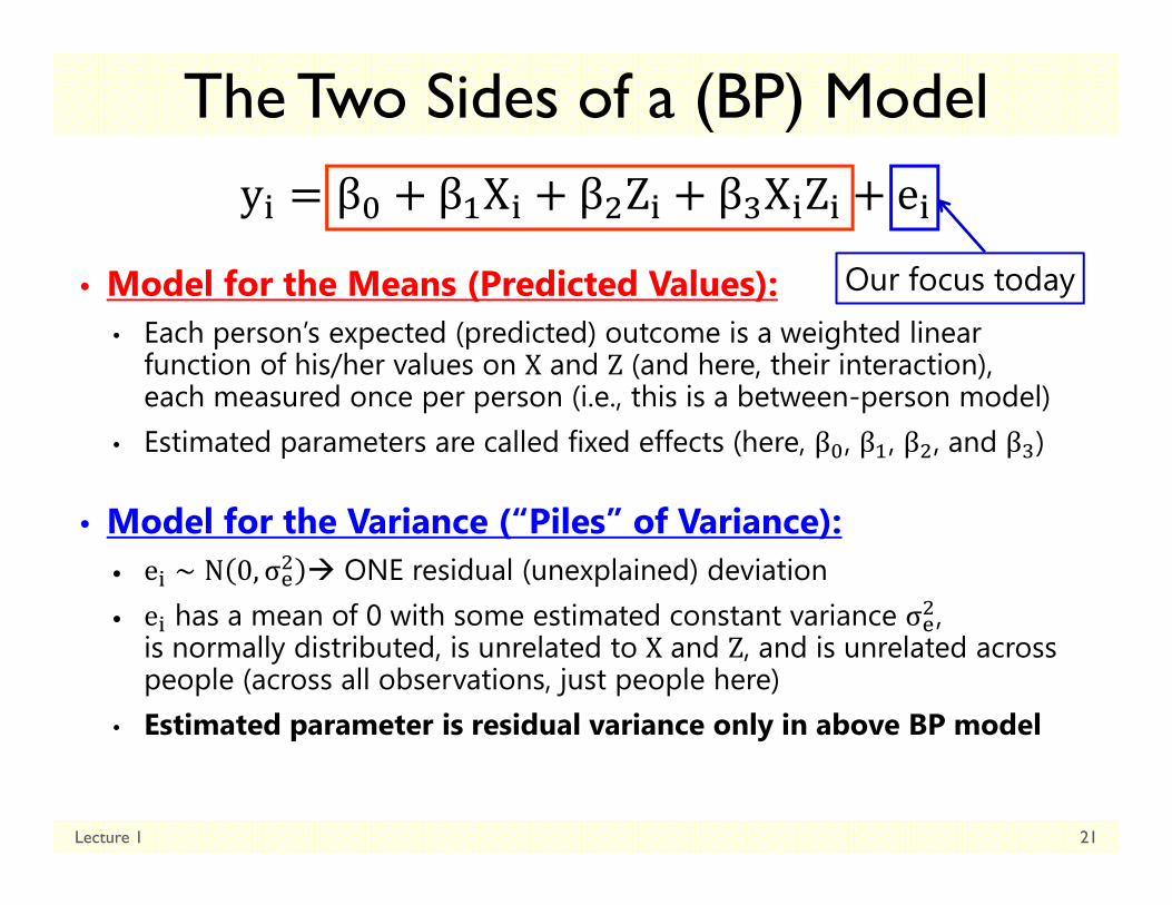
The Two Sides of a (BP) Model

• Model for the Means (Predicted Values):• Each person’s expected (predicted) outcome is a weighted linear

function of his/her values on X and Z (and here, their interaction), each measured once per person (i.e., this is a between-person model)

• Estimated parameters are called fixed effects (here, β , β , β , and β )

• Model for the Variance (“Piles” of Variance):• e ∼ N 0, σ ONE residual (unexplained) deviation• e has a mean of 0 with some estimated constant variance σ ,

is normally distributed, is unrelated to X and Z, and is unrelated across people (across all observations, just people here)

• Estimated parameter is residual variance only in above BP model

Lecture 1 21

Our focus today

An Empty Between-Person Model (i.e., Single-Level)

Lecture 1 22

20

40

60

80

100

120

140

Mean = 89.55Std. Dev. = 15.114N = 1,334

yi = β0 + ei

Filling in values:32 = 90 + −58

Model for the Means

error variance:

y

Adding Within-Person Information… (i.e., to become a Multilevel Model)

Lecture 1 23

Full Sample Distribution

20

40

60

80

100

120

140

Mean = 89.55Std. Dev. = 15.114N = 1,334

3 People, 5 Occasions each

Now yi per person becomes yti per

time per person…

Empty +Within-Person Model for yti

Start off with mean of yti as “best guess” for any value:

= Grand Mean

= Fixed Intercept

Can make better guess by taking advantage of repeated observations:

= Person Mean

Random Intercept

Lecture 1 24

140

120

100

80

60

40

20

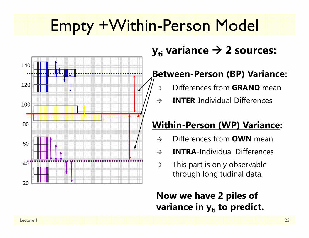
Empty +Within-Person Modelyti variance 2 sources:

Between-Person (BP) Variance: Differences from GRAND mean

INTER-Individual Differences

Within-Person (WP) Variance: Differences from OWN mean

INTRA-Individual Differences

This part is only observable through longitudinal data.

Now we have 2 piles of variance in yti to predict.

Lecture 1 25

140

120

100

80

60

40

20

Hypothetical Longitudinal Data(black line = sample mean)

Lecture 1 26

“Error” in a BP Model for the Variance:Single-Level Model

Lecture 1 27

eti represents all yti variance

e1ie2i e3i

e4ie5i

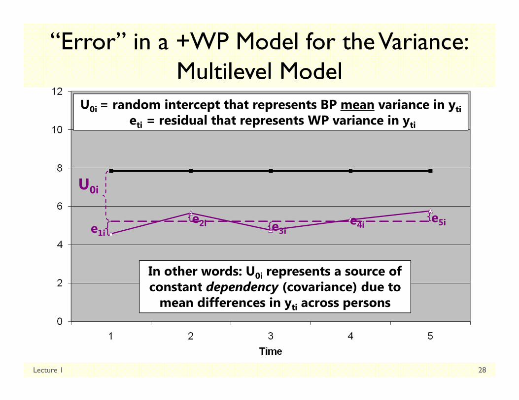
“Error” in a +WP Model for the Variance:Multilevel Model

Lecture 1 28

U0i

U0i = random intercept that represents BP mean variance in ytieti = residual that represents WP variance in yti

e1ie2i e3i

e4i e5i

In other words: U0i represents a source of constant dependency (covariance) due to

mean differences in yti across persons

Empty +Within-Person Modelyti variance 2 sources:

Level 2 Random Intercept Variance (of U0i, as ):

Between-Person Variance

Differences from GRAND mean

INTER-Individual Differences

Level 1 Residual Variance(of eti, as ):

Within-Person Variance

Differences from OWN mean

INTRA-Individual Differences

Lecture 1 29

140

120

100

80

60

40

20

U0i

U0ieti

eti

eti

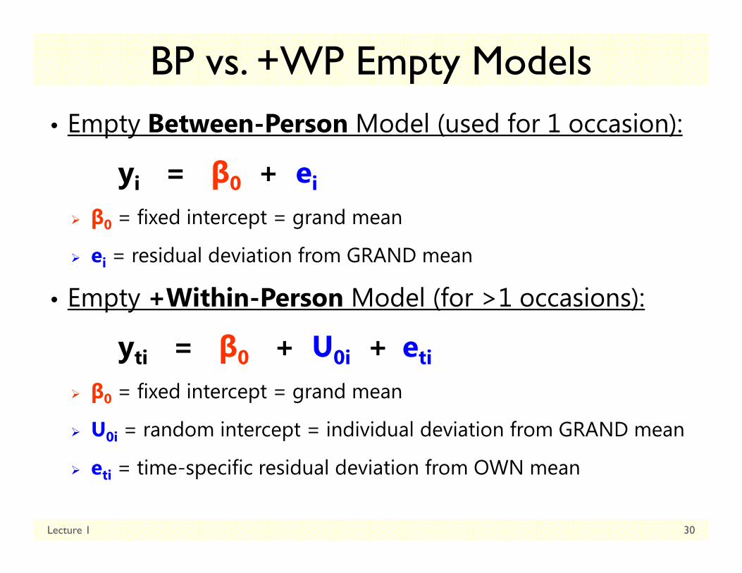
BP vs. +WP Empty Models• Empty Between-Person Model (used for 1 occasion):

yi = β0 + ei

β0 = fixed intercept = grand mean

ei = residual deviation from GRAND mean

• Empty +Within-Person Model (for >1 occasions):

yti = β0 + U0i + eti

β0 = fixed intercept = grand mean

U0i = random intercept = individual deviation from GRAND mean

eti = time-specific residual deviation from OWN mean

Lecture 1 30

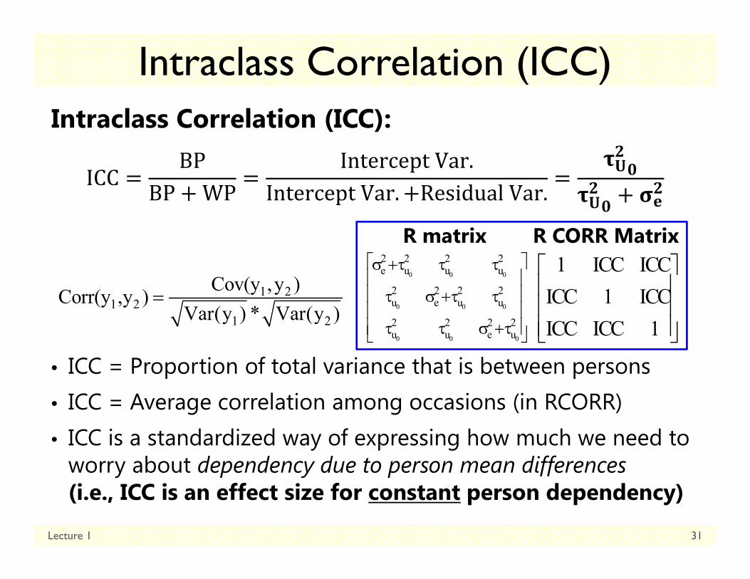
Intraclass Correlation (ICC)Intraclass Correlation (ICC):

ICCBP

BP WPInterceptVar.

InterceptVar. ResidualVar.

• ICC = Proportion of total variance that is between persons• ICC = Average correlation among occasions (in RCORR)• ICC is a standardized way of expressing how much we need to

worry about dependency due to person mean differences(i.e., ICC is an effect size for constant person dependency)

Lecture 1 31

0 0 0

0 0 0

0 0 0

2 2 2 2e u u u

2 2 2 2u e u u

2 2 2 2u u e u

1 ICC ICCICC 1 ICCICC ICC 1

R matrix R CORR Matrix

1 21 2

1 2

Cov(y ,y )Corr(y ,y )Var(y ) * Var(y )

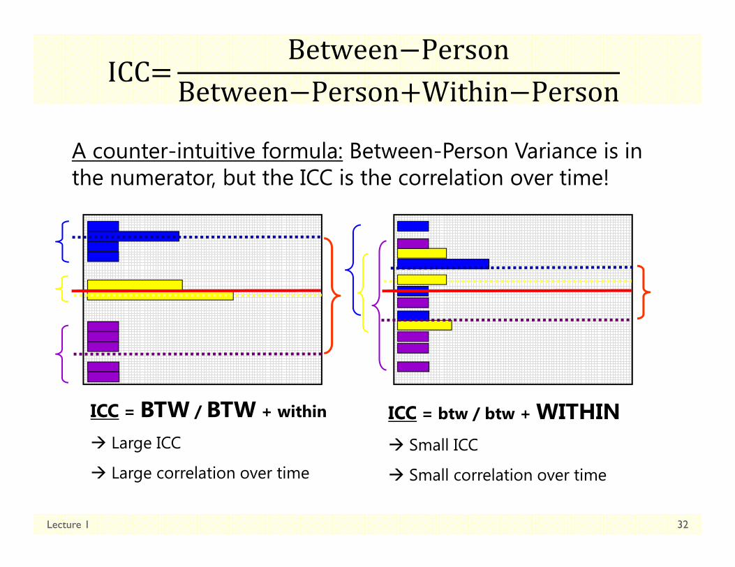
Lecture 1 32

A counter-intuitive formula: Between-Person Variance is in the numerator, but the ICC is the correlation over time!

ICC = BTW / BTW + within

Large ICC

Large correlation over time

ICC = btw / btw + WITHIN Small ICC

Small correlation over time

BP and +WP Conditional Models• Multiple Regression, Between-Person ANOVA: 1 PILE yi = (β0 + β1Xi + β2Zi…) + ei

ei ONE residual, assumed uncorrelated with equal variance across observations (here, just persons) “BP (all) variation”

• Repeated Measures, Within-Person ANOVA: 2 PILES yti = (β0 + β1Xi + β2Zi…) + U0i + eti

U0i A random intercept for differences in person means, assumed uncorrelated with equal variance across persons “BP (mean) variation”= is now “leftover” after predictors

eti A residual that represents remaining time-to-time variation, usually assumed uncorrelated with equal variance across observations (now, persons and time) “WP variation”= is also now “leftover” after predictors

Lecture 1 33


Lecture 1 34


Likelihood-Based Model Comparisons (briefly)

• Relative model fit is indexed by a “deviance” statistic −2LL Log of likelihood (LL = total data height) of observing the data given model

parameters; −2*LL so that the differences between model LL values follow ~χ −2LL is a measure of BADNESS of fit, so smaller values = better models Two flavors (labeled as −2 log likelihood in SAS, SPSS, but given as LL instead in

STATA and Mplus): Maximum Likelihood (ML) or Restricted (Residual) ML (REML)

• Nested models are compared using their deviance values: −2∆LL Test (i.e., Likelihood Ratio Test, Deviance Difference Test)

1. Calculate −2∆LL: (−2LLfewer) – (−2LLmore)2. Calculate ∆df: (# Parmsmore) – (# Parmsfewer)3. Compare −2∆LL to χ2 distribution with df = ∆df

CHIDIST in excel will give exact p-values for the difference test; so will STATA

• Add parameters? Model fit can be BETTER (signif) or NOT BETTER • Remove parameters? Model fit can be WORSE (signif) or NOT WORSE

Lecture 1 35

1. & 2. must be positive values!

Example Data for BP and WP Models• 50 kids in a control or treatment group each measured twice• Hypothesis: Learning outcome should be higher at post-test

than pre-test, with a greater difference in the treatment group

Lecture 1 36

Means (SE) Pre-Test Post-Test Marginal

Control 49.08 (1.14) 54.90 (1.13) 51.99 (0.89)

Treatment 50.76 (0.91) 58.62 (0.99) 54.70 (0.87)

Marginal 49.92 (0.73) 56.76 (0.79) 53.34 (0.64)6.84

2.711.68 3.72

5.82

7.86

2.04

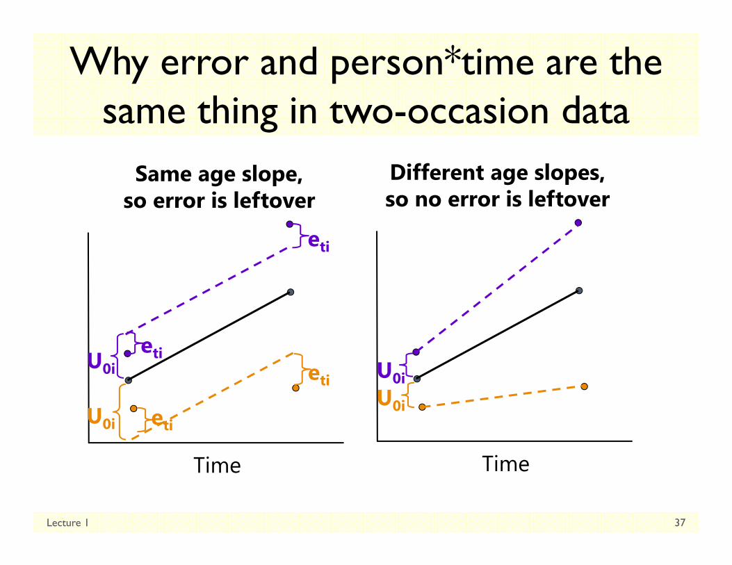
Why error and person*time are the same thing in two-occasion data

Lecture 1 37

Time

U0i

U0i

eti

eti

eti

eti

Time

U0iU0i

Same age slope, so error is leftover

Different age slopes, so no error is leftover

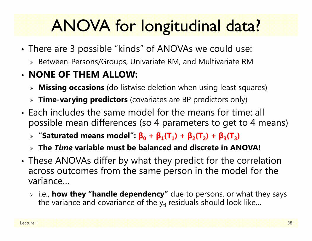
ANOVA for longitudinal data?• There are 3 possible “kinds” of ANOVAs we could use:

Between-Persons/Groups, Univariate RM, and Multivariate RM

• NONE OF THEM ALLOW: Missing occasions (do listwise deletion when using least squares) Time-varying predictors (covariates are BP predictors only)

• Each includes the same model for the means for time: all possible mean differences (so 4 parameters to get to 4 means) “Saturated means model”: β0 + β1(T1) + β2(T2) + β3(T3) The Time variable must be balanced and discrete in ANOVA!

• These ANOVAs differ by what they predict for the correlation across outcomes from the same person in the model for the variance… i.e., how they “handle dependency” due to persons, or what they says

the variance and covariance of the yti residuals should look like…

Lecture 1 38

1. Between-Groups ANOVA• Uses eti only (total variance = a single variance term of σ )• Assumes no covariance at all among observations from the

same person: Dependency? What dependency?• Will usually be very, very wrong for longitudinal data

WP effects tested against wrong residual variance (significance tests will often be way too conservative)

Will also tend to be wrong for clustered data, but less so (because the correlation among persons from the same group is not as strong as the correlation among occasions from the same person)

• Predicts a variance-covariance matrixover time (here, 4 occasions) like this, called “Variance Components”(R matrix is TYPE=VC on REPEATED):

Lecture 1 39

2e

2e

2e

2e

σ 0 0 0

0 σ 0 0

0 0 σ 0

0 0 0 σ

R matrix

2a. Univariate Repeated Measures• Separates total variance into two sources:

Between-Person (mean differences due to U0i, or across persons)

Within-Person (remaining variance due to eti, or across time, person)

• Predicts a variance-covariance matrixover time (here, 4 occasions) like this, called “Compound Symmetry”(R matrix is TYPE=CS on REPEATED): Mean differences from U0i are the only

reason why occasions are correlated

• Will usually be at least somewhat wrong for longitudinal data If people change at different rates,

the variances and covariancesover time have to change, too

Lecture 1 40

0 0 0 0

0 0 0 0

0 0 0 0

0 0 0 0

2 2 2 2 2e u u u u

2 2 2 2 2u e u u u

2 2 2 2 2u u e u u

2 2 2 2 2u u u e u

TimeTime

R matrix

The Problem with Univariate RM ANOVA

• Univ. RM ANOVA τ σ predicts compound symmetry: All variances and all covariances are equal across occasions

In other words, the amount of error observed should be the same at any occasion, so a single, pooled residual variance term makes sense

If not, tests of fixed effects may be biased (i.e., sometimes tested against too much or too little error, if error is not really constant over time)

COMPOUND SYMMETRY RARELY FITS FOR LONGITUDINAL DATA

• But to get the correct tests of the fixed effects, the data must only meet a less restrictive assumption of sphericity: In English pairwise differences between adjacent occasions have equal

variance and covariance (satisfied by default with only 2 occasions)

If compound symmetry is satisfied, so is sphericity (but see above)

Significance test provided in ANOVA for where data meet sphericity assumption

Other RM ANOVA approaches are used when sphericity fails…

Lecture 1 41

The Other Repeated Measures ANOVAs…• 2b. Univariate RM ANOVA with sphericity corrections

Based on ε how far off sphericity (from 0-1, 1=spherical) Applies an overall correction for model df based on estimated ε,

but it doesn’t really address the problem that data ≠ model

• 3. Multivariate Repeated Measures ANOVA All variances and covariances are estimated

separately over time (here, n = 4 occasions), called “Unstructured” (R matrix is TYPE=UN on REPEATED)—it’s not a model, it IS the data:

Because it can never be wrong, UN can be useful for complete and balanced longitudinal data with few (e.g., 2-4) occasions (n)

Parameters = ∗

so it can be hard to estimate with many occasions

Unstructured can also be specified to include random intercept variance τ

All other models for the variance are nested under Unstructured, so we can do LRT model comparisons to see if any other model is NOT WORSE

Lecture 1 42

211 12 13 14

221 22 23 24

231 32 33 43

241 42 43 44

σ σ σ σ

σ σ σ σ

σ σ σ σ

σ σ σ σ

R matrix

Summary: ANOVA approaches for longitudinal data are “one size fits most”

• Saturated Model for the Means (balanced time required) All possible mean differences

Unparsimonious, but best-fitting (is a description, not a model)

• 3 kinds of Models for the Variance (need complete data in least squares) BP ANOVA (σ only) assumes independence and constant variance over time

Univ. RM ANOVA τ σ assumes constant variance and covariance

Multiv. RM ANOVA (whatever) no assumptions; is a description, not a model

• MLM will give us more flexibility in both parts of the model: Fixed effects that predict the pattern of means (polynomials, pieces)

Random intercepts and slopes and/or alternative covariance structures that predict intermediate patterns of variance and covariance over time

Lecture 1 43

there is no structure that shows up in a scalar equation (i.e., the way U0i + eti does)

Introduction to Multilevel Models for Longitudinal Data · Introduction to Multilevel Models for...

Documents

Transcript of Introduction to Multilevel Models for Longitudinal Data · Introduction to Multilevel Models for...