Ivan Markov

INTRODUCTION TO MATRIX CALCULUS

Sofia 2011

1. Introduction to the Linear Algebra

The objective of this chapter is to present the fundamentals of matrices, with emphasis on those aspects that are important in finite element analysis. This is just a review of matrix algebra and should be known to the student from a course in linear algebra.

Of course, only a rather limited discussion of matrices and tensors is given here, but we hope that the focused practical treatment will provide a strong basis for understanding the finite element formulations given later. 1.1 Matrices. Basic Concepts Further in our exposition with will be denoted the set of real numbers, and is the real n-dimensional vector space. The concept vector space is a fundamental in the theory of matrices but now we use it intuitively, and later we will give its definition. Matrices defined on the field of real numbers are mainly used in this book.

n

From a simplistic point of view, matrices can simply be taken as ordered arrays (tables) of numbers that are subjected to specific rules of addition, multiplication, and so on. It is of course important to be thoroughly familiar with these rules, and we review them in this chapter.

However, by far more interesting aspects of matrices and matrix algebra are recognized when we study how the elements of matrices are derived in the analysis of a physical problem and why the rules of matrix algebra are actually applicable. In this context, the use of tensors and their matrix representations are important and provide a most interesting subject of study.

Of course, only a rather limited discussion of matrices and tensors is given here, but we hope that the focused practical treatment will provide a strong basis for understanding the finite element formulations given later. Definition: A matrix is an array (table) of ordered numbers. A general matrix consists of mn numbers arranged in m rows and n columns, giving the following array

. (1.1)

11 12 1

21 22 2

1 2

n

nm n ij

m m mn

a a a

a a aA a

a a a

A A

We say that this matrix has order (m by n). If mm n n , the matrix is square with order n. With

we denote an arbitrary element of the matrix, which belongs to the ith row and to the jth column.

The matrix elements with , i.e. are called a principal diagonal of the matrix A. When

we have only one row (m = 1) or one column (n = 1), we also call A a vector. Therefore the following one dimensional array

ija

ija i j iia

1

2

n

x

xx

x

x

(1.2)

is a vector. We use the notation . Further in this book we consider all vectors as columns. The numbers

nx 1 2, , , nx x x are components of the vector.

2

According to the definition we consider that 0, if 0 for 1, 2,ix i n x , (1.3)

0, if 0 for 1, 2,ix i n x . (1.4)

The effectiveness of using matrices in practical calculations is readily realized by considering the of a set of linear simultaneous equations such as

1 2 3

1 2 3

1 2 3 4

3 4

10 4 2 = 18

4 12 = 14

2 15

20 18

x x x

x x x

x x x x

x x

30

(1.5)

This set of linear algebraic equations can be written as follows

. (1.6)

1

2

3

4

10 4 2 0 18

4 12 1 0 14

2 1 15 1 30

0 0 1 20 18

x

x

x

x

xA b

where the unknowns are 1 2 3 4, , and x x x x . Using matrix notation, this set of equations is written

more compactly as , (1.7) Ax b where A is the matrix of the coefficients in the set of linear equations, x is the matrix of unknowns, and b is the matrix of known quantities. A comma between subscripts will be used when there is any risk of confusion, e.g., . 2, 1i ja

Definition: The transpose of the m n matrix A, written as , is obtained by interchanging the rows and columns in A If

TAT A A , it follows that the number of rows and

columns in A are equal and that . Because, ij jia a m n we say that A is a square matrix of order

n, and because , we say that A is a symmetric matrix. Note that symmetry implies that A is

square, but not vice versa; i.e., a square matrix need not be symmetric. Obviously ij jia a

TT A A .

The process of transposing is clear from the following example:

4 3

4 1 3

2 15 6

16 1 9

3 2 1

A ,

3 4

4 2 16 3

1 15 1 2

3 6 9 1

T

A . (1.8)

Definition: The matrices A and B are equal if and only if they have the same number or rows and columns and all corresponding elements are equal, i.e., ij ija b for all i and j.

3

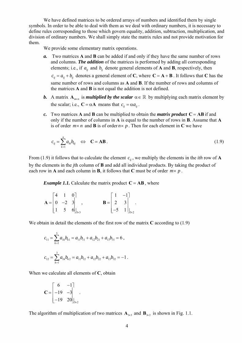
We have defined matrices to be ordered arrays of numbers and identified them by single symbols. In order to be able to deal with them as we deal with ordinary numbers, it is necessary to define rules corresponding to those which govern equality, addition, subtraction, multiplication, and division of ordinary numbers. We shall simply state the matrix rules and not provide motivation for them.

We provide some elementary matrix operations.

a. Two matrices A and B can be added if and only if they have the same number of rows and columns. The addition of the matrices is performed by adding all corresponding elements; i.e., if ija and ijb denote general elements of A and B, respectively, then

denotes a general element of C, where ij ij ijc a b C A B . It follows that C has the

same number of rows and columns as A and B. If the number of rows and columns of the matrices A and B is not equal the addition is not defined.

b. A matrix m nA is multiplied by the scalar by multiplying each matrix element by

the scalar; i.e., C A means that ij ijc a .

c. Two matrices A and B can be multiplied to obtain the matrix product C AB if and only if the number of columns in A is equal to the number of rows in B. Assume that A is of order m n and B is of order n p . Then for each element in C we have

. (1.9) 1

n

ij ikk

c a C ABkjb

From (1.9) it follows that to calculate the element , we multiply the elements in the ith row of A

by the elements in the jth column of B and add all individual products. By taking the product of each row in A and each column in B, it follows that C must be of order .

ijc

m p Example 1.1. Calculate the matrix product C AB , where

,

3 3

4 1 0

0 2 3

1 5 6

A

3 2

1 1

2 3

5 1

B .

We obtain in detail the elements of the first row of the matrix C according to (1.9)

, 3

11 1 1 11 11 12 21 13 311

6k kk

c a b a b a b a b

. 3

12 1 2 11 12 12 22 13 321

1k kk

c a b a b a b a b

When we calculate all elements of C, obtain

.

3 2

6 1

19 3

19 20

C

The algorithm of multiplication of two matrices 3 3A and 3 2B is shown in Fig. 1.1.

4

1j

5

Fig. 1.1. Matrix multiplication The procedure for matrix multiplication, shown in Fig. 1.1 is only convenient for “in hand” calculations and also for easily writing of algebraic and differential equations using matrix notations. The multiplication of a matrix m nA by nx is identical to the multiplication of the

matrices и . The given definitions allow to verify the correctness of the transformation of

equations (1.5) into the form (1.6). m nA 1nx

As is well known, the multiplication of ordinary numbers is commutative; i.e., ab = ba. We need to investigate if the same holds for matrix multiplication. Let us consider the matrices

и 2

5

A 1 2B .

We calculate the matrix products

, 2 4

5 10

AB 12 12 BA .

Therefore, the products AB and BA are not the same, and it follows that matrix multiplication is not commutative. Indeed, depending on the orders of A and B, the orders of the two product matrices AB and BA can be different, and the product AB may be defined, whereas the product BA

may not be calculable (this can be easily inspected for the matrices A and B in example 1.1. If the matrices A and B satisfy AB BA , we say that A и B commute.

The distributive law is valid and it states that

+

11b

21a 22a 23a 21c

21b

31b

21 11a b

23 31a b

B 22 21a b

2i C

A

21 21 11 22 21 23 31c a b a b a b

. (1.10) A B C AB AC

This law holds if the operations in (1.10) are defined. The associative law states that , (1.11) A BC AB C

in other words, that the order of multiplication is insignificant. In addition to being noncommutative, matrix algebra differs from scalar algebra in other ways. The cancellation of matrices in matrix equations also cannot be performed, in general, as the cancellation of ordinary numbers. In particular, the equality AB AC does not necessarily imply

, since algebraic summing is involved in forming the matrix products. As another example, if the product of two matrices is a null matrix, that is, B C

AB 0 , the result does not necessarily imply that either A or B is a null matrix. However, it must be noted that A C if the equation AB CB holds for all possible B. Namely, in that case, we simply select B to be the identity matrix I, and hence . A C The proof of above laws is carried out by using the definition of matrix multiplication in (1.9). Definition: A null matrix (also known as a zero matrix) is a matrix of any order in which the value of all elements is 0.

Definition: An identity (or unit) matrix I, which is a square matrix of order n with only zero elements except for its diagonal entries, which are unity. For example, the identity matrix of order 3 is

. (1.12)

1 0 0

0 1 0

0 0 1

I

It can be easily seen that arbitrary matrices A and B satisfy the following equations , , , (1.13) A0 0A 0 AI = A IB = B if the corresponding matrix operations are defined. It can be easily shown that the transpose of the product of two matrices A and B is equal to the product of the transposed matrices in reverse order; i.e.,

. (1.14) T T TAB B A

The proof that (1.14) does hold is obtained using the definition for the evaluation of a matrix product given in (1.9).

Definition: A symmetric matrix is a square matrix ija A composed of elements such

that the nondiagonal values are symmetric about the principal diagonal. Mathematically, symmetry is expressed as . If the matrix A is symmetric then , for ,ij jia a i j T A A .

6

For an arbitrary matrix A the products и are symmetric matrices. Това се вижда от равенството

TA A TAA

7

T

. (1.15) T TT T T AA A A AA

For example, if

, then 1 2 3

4 5 6

A14 32

32 77T

AA and .

17 22 27

22 29 36

27 36 45

T

A A

It should be noted that although A and B may be symmetric, AB is, in general, not

symmetric. The following example demonstrates this observation

, 2 1

1 3

A 3 1

1 1

B , 5 1

0 2

AB .

If A is symmetric, the matrix is always symmetric. The proof follows using (1.14): TB DB

, T TT T B DB DB B B D BT T

But, because , we have T D D

. (1.16) TT TB DB B DB

and hence is symmetric. In particular, we can obtain (1.15) from (1.16) in case of . TB DB D = I If the elements of the matrix m nA are differentiable functions of one or several variables the

differentiation of the matrix is performed according to the rule

ija

x x

A

, (1.17)

and the integration is defined as

. (1.18) b b

ij

a a

dx a dx

A

It is clear from (1.17) and (1.18) that the matrix differentiation and the integration are operations applied to each matrix element. 1.2 Special types of matrices Whenever the elements of a matrix obey a certain law, we can consider the matrix to be of special form. A real matrix is a matrix whose elements are all real. A complex matrix has elements that may be complex. We shall deal only with real matrices.

A diagonal matrix is a square matrix composed of elements such that .

Therefore, the only nonzero terms are those on the main diagonal (upper left to lower right). Sometimes the diagonal matrix is written as

0 if ija i j

. iidiag dD

Schematically the diagonal matrix is shown in Fig. 1.2.a. All matrix elements which are not hatched are zeroes.

1

8

b. Banded matrix

a. Diagonal matrix d. upper triangular c. lower triangular matrix matrix f. “sky line” matrix e. three diagonal matrix

Fig. 1.2 Special types of matrices

A square matrix A is banded (Fig. 1.2.b) if it is satisfy the following conditions

9

j

1

, (1.19) 0 за и за ija j i i where 2 is the bandwidth of A. As an example, the following matrix is a symmetric banded matrix of order 5. The half-bandwidth Δ is 2:

.

4 1 2 0 0

1 5 1 1 0

2 1 12 1 1

0 1 1 9 2

0 0 1 2 10

A

If the half-bandwidth of a matrix is zero, we have nonzero elements only on the diagonal of the matrix and denote it as a diagonal matrix. For example, the identity matrix is a diagonal matrix. The matrices shown in Fig. 1.2.c and in Fig. 1.2.d are called a lower triangular matrix and a upper triangular matrix. A symmetric matrix in Fig. 1.2.f is “skyline” matrix. All elements which are outside the skyline are zeroes. The finite element method problems very often use large scale skyline matrices.

In computer calculations with matrices, we need to use a scheme of storing the elements of the matrices in computer memory. An obvious way of storing the elements of a matrix A of order

is simply to dimension in the program an array m n A m n , and store each matrix element

in the storage location ija

A i j . However, in many calculations we store in this way unnecessarily

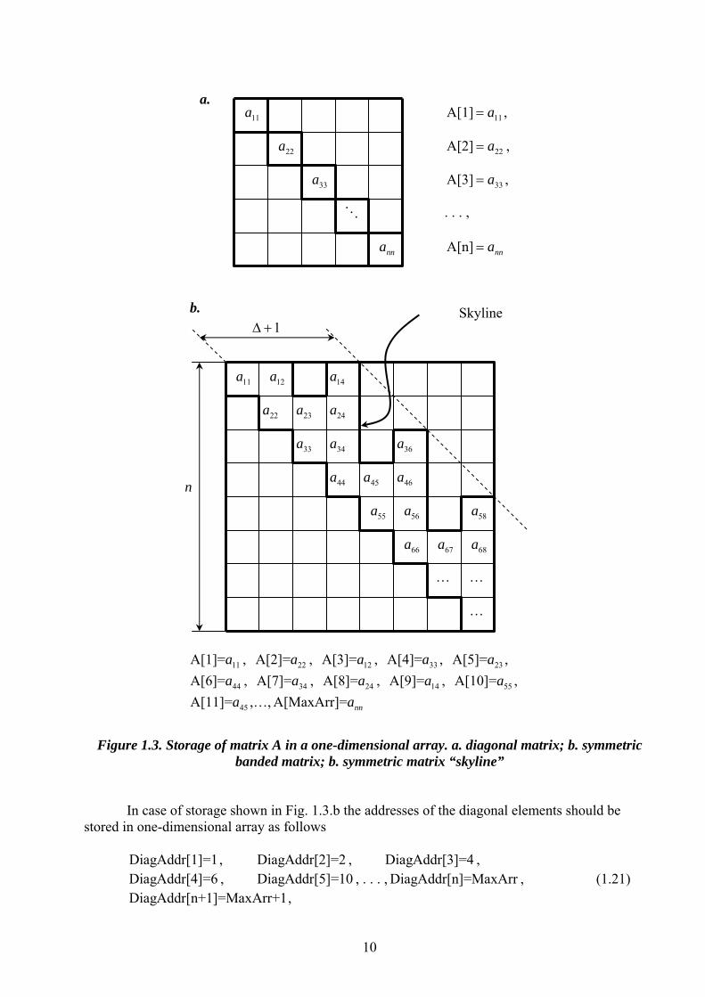
many zero elements of A, which are never needed in the calculations. Also, if A is symmetric, we should probably take advantage of it and store only the upper half of the matrix, including the diagonal elements. In general, only a restricted number of high-speed storage locations are available, and it is necessary to use an effective storage scheme in order to be able to take into high-speed core the maximum matrix size possible. If the matrix is too large to be contained in high-speed storage, the solution process will involve reading and writing on secondary storage, which can add significantly to the solution cost. Fortunately, in finite element analysis, the system matrices are symmetric and banded. Therefore, with an effective storage scheme, rather large-order matrices can be kept in high-speed core. A diagonal matrix А of order n is stored in one-dimensional array A i , 1,2, ,iia i n . (1.20)

This way of storage is shown in Fig. 1.3.a.

Consider a banded matrix as shown in Fig. 1.3.b. The zero elements within the "skyline" of the matrix may be changed to nonzero elements in the solution process; for example, may be a

zero element but becomes nonzero during the solution process. The zero elements that are outside the skyline are always zeroes after the transformation has been performed. Therefore we allocate storage locations to zero elements within the skyline but do not need to store zero elements that are outside the skyline. The storage scheme that will be used in the finite element solution process is indicated in Fig. 1.3.b. Of course, there are different schemes for matrix storage in the FEM.

46a

a. 11a

11A[1] a ,

22a 22A[2] a ,

33a 33A[3] a , . . . ,

nna A[n] nna b. Skyline

10

n

11a 12a

22a 23a

14a

24a

46a

66a

33a 34a

44a 45a

36a

55a 56a

67a

58a

…

68a

…

…

1

11A[1]=a , , , , , 22A[2]=a 12A[3]=a 33A[4]=a 23A[5]=a

44A[6]=a , , , , , 34A[7]=a 24A[8]=a 14A[9]=a 55A[10]=a

45A[11]=a ,…, A[MaxArr]= nna

Figure 1.3. Storage of matrix A in a one-dimensional array. a. diagonal matrix; b. symmetric banded matrix; b. symmetric matrix “skyline”

In case of storage shown in Fig. 1.3.b the addresses of the diagonal elements should be stored in one-dimensional array as follows , , , DiagAddr[1]=1 DiagAddr[2]=2 DiagAddr[3]=4 , , . . . , , (1.21) ,

DiagAddr[4]=6DiagAddr[n+1]=

DiagAddr[5]=10xArr+1

DiagAddr[n]=MaxArrMa

where MaxArr is the total number of elements within skyline. 1.3 Determinant and Trace of a Matrix A mathematical object consisting of many components usually is characterized (evaluated) by means of one number (scalar). Typical examples are the trace and determinant of a matrix. The trace and determinant of a matrix are defined only if the matrix is square. Both quantities are single numbers, which are evaluated from the elements of the matrix and are therefore functions of the matrix elements. Mainly two approaches use in the determinant definition. Here we represent the definition according to the determinant of the matrix n nA is calculating by using the determinants of lower

order matrices. Definition:

a. The determinant of a matrix of order 1 (n=1) is simply the element of the matrix; i.e., if 11a , then 11A det aA .

b. If i is an arbitrary row of the matrix n nA , then the determinant det A is

calculated as follows

1

det 1 detn

i j

ij ijj

a

A A , (1.22)

where is the matrix of order ijA 1n n 1

A

resulting from the deletion of the row i

and the column j of A. The equation (1.22) is known as Laplace decomposition along ith row. By analogy if we use Laplace decomposition along jth column we obtain

. (1.23) 1

det 1 detn

i j

ij iji

a

A

Note that det are the determinants of the ijA 1n order matrices obtained by striking out the ith

row and the jth column for given j. These are known as minors. A minor of a determinant is another determinant formed by removing an equal number of rows and columns from the original determinant. Example: Evaluate the determinant of A, where

11 12

21 22

a a

a a

A

Using the relation (1.22), we obtain 11 22aA , 12 21aA ,

, 1 1 1 2

11 11 12 12det 1 det 1 deta a A A A

but , 11 22det aA 12 21det aA .

Hence

11

. (1.24) 11 22 12 21det a a a a A

This relation is the general formula for the determinant of a 2 2 matrix. Using the recurrence relation (1.22) along the row 1 (i=1) for the matrix

11 12 13

21 22 23

31 32 33

a a a

a a a

a a a

A

we obtain

, 22 2311

32 33

a a

a a

A 21 2312

31 33

a a

a a

A , 21 2213

31 32

a a

a a

A .

According to formula (1.24) , 11 22 33 23 32det a a a a A

, 12 21 33 23 31det a a a a A

. 13 21 32 22 31det a a a a A

Then from (1.22) we can write

. 1 1 1 2 1 3

11 11 12 12 13 13det 1 det 1 det 1 deta a a A A A A

After substituting de into the previous equation we obtain t ijA

. (1.25) 11 22 33 12 23 31 13 21 32

11 23 32 12 21 33 13 22 31

det a a a a a a a a a

a a a a a a a a a

A

In such a way we have obtained known formulae (1.24) and (1.25) for the determinant of 3 3 matrix. We shall remember some fundamental properties of the determinants without proof. 1. de . t detT A A 2. de . t 1I 3. The determinant of the matrix product is . (1.26) det det detAB A B

4. The determinant of a diagonal matrix iidiag dD is

. 11 22det nnd d dD

12

5. The determinant of the lower triangular matrix or of the upper triangular matrix is equal to the product of diagonal terms. The solution of a system of linear algebraic equations uses the specific decomposition TA LDL

t 1,

where L is a lower unit triangular matrix (the diagonal elements of L are equal to 1 and de L ) and D is a diagonal matrix. In that case, , (1.27) det det det det TA L D L

A

and because de , we have t 1L . (1.28) 11 22det det nnd d d A D 6. If α is a scalar, then . (1.29) det detn A

Definition: The trace of the square matrix A of order n is denoted as tr(A) and is equal to

. (1.30) 1

n

iii

tr Sp a

A A

1.4 Matrix Inversion Definition: The inverse of a matrix A is denoted by 1A . Assume that the inverse exists; then the elements of 1A are such that , (1.31) 1 1 AA A A I where I is the identity matrix. The inverse of a matrix does not need to exist. A trivial example is the null matrix. Definition: A square matrix A is said to be nonsingular if det 0A . A matrix A is a

singular matrix if det 0A .

Theorem: Each nonsingular matrix possesses an inverse. We shall describe some properties of the inverse: 1. Determinant of the inverse of matrix. It can be easily obtained by using the definition (1.31) and the relation (1.26) . Therefore

1 1det det det 1 A A I A A I

1 1det

det A

A. (1.32)

2. The inverse of the product of matrices

13

. (1.33) 1 1 1 AB B A

3. The inverse of the transposed matrix

11 T T A A . (1.34)

4. The inverse of a symmetric matrix is also symmetric.

If the inverse of matrix A can be determined, we can multiply both sides of Equation (1.7) by the inverse to obtain the solution for the simultaneous equations directly as 1A . (1.35) -1x = A b However, the inversion of A is very costly, and it is much more effective to only solve the equations in (1.7) without inverting A. Indeed. although we may write symbolically that , to evaluate x we actually only solve the equations.

-1x = A b

One way of calculating the inverse 1А of a matrix A of order n is in terms of its

determinant. If are the elements of the inverse, i.e., ij1

ij β A , then they are calculated as

follows

det

1det det

i j ji jiij

A

A A, , 1,2, ,i j n , (1.36)

where is the submatrix of order jiA 1n n 1 resulting from the deletion of the row j and the

column i of A. We have to notice that the quantities are known as adjoints of

A.

1 deti j

ji ji

A

Calculation of the inverse of a matrix per Equation (1.36) is cumbersome and not very practical. Formulae (1.36) are convenient for matrices of low order ( 3n ). That is why we represent here a general algorithm for calculating the inverse 1A . Let A and are square matrices of order n that satisfy the following matrix equation

β

, (1.37) Aβ = I where I is an identity matrix. Then 1β = A . For the solution of each system of equations in (1.37), we can use the well known algorithms for solution of a system of linear algebraic equations. Let

are vector columns of the matrix β and are vector columns of the unite

matrix, i.e., 1 2, , , nβ β β 1 2, , , ne e e

, ,

1

2

i

ii

ni

β

0

1

0

i row i

e

then each column of the inverse β is obtained as a result of solution of the system of equations iβ

14

15

n . (1.38) , 1,2, ,i i i Aβ e After the solution the ith system of equations (1.38) is performed, the solution vector is put in

the ith column of the inverse iβ

1 A β Example 1.2. Calculate the inverse 1β = A where

1 1 0

1 2 1

0 1 2

A

The identity matrix I of the third order and its vector-columns are respectively ie

, 1 2 3

1 0 0

0 1 0

0 0 1

I e e e 1

1

0

0

e , 2

0

1

0

e , . 3

0

0

1

e

Using a computer program for each 1,2,3i we solve the systems of equations i iAβ e

and obtain

1

3

2

1

β , , 2

2

2

1

β 3

1

1

1

β .

After the solution is made we arrange 1,2,3i i β in the columns of , and hence 1β A

. 11 2 3

3 2 1

2 2 1

1 1 1

β A β β β

1.5 Matrix Partitioning

Any matrix can be subdivided or partitioned into a number of submatrices of lower order.

The concept of matrix partitioning is most useful in reducing the size of a system of equations and accounting for specified values of a subset of the dependent variables. A submatrix is a matrix that is obtained from the original matrix by including only the elements of certain rows and columns. The idea is demonstrated using a specific case in which the dashed lines are the lines of partitioning

11 12 13 14 15 16

21 22 23 24 25 26

31 32 33 34 35 36

41 42 43 44 45 46

a a a a a a

a a a a a a

a a a a a a

a a a a a a

A

, (1.39)

It should be noted that each of the partitioning lines must run completely across the original matrix. Using the partitioning, matrix A is written as

, (1.40) 11 12 13

21 22 23

A A AA

A A A

where

, , 1111

21

a

a

A 12 13 1412

22 23 24

a a a

a a a

A 15 1613

25 26

a a

a a

A , . . . (1.41)

ijA are called submatrices of the matrix A.

The partitioning of matrices can be of advantage in saving computer storage; namely, if

submatrices repeat, it is necessary to store the submatrix only once. The same applies in arithmetic. Using submatrices, we may identify a typical operation that is repeated many times. We then carry out this operation only once and use the result whenever it is needed.

The rules to be used in calculations with partitioned matrices follow from the definition of matrix addition, subtraction, and multiplication. Using partitioned matrices we can add, subtract, or multiply as if the submatrices were ordinary matrix elements, provided the original matrices have been partitioned in such a way that it is permissible to perform the individual submatrix additions, subtractions, or multiplications.

The rules for partitioned matrices are analogous to rules for ordinary matrices. It should be noted that the partitioning of the original matrices is only an approach to facilitate matrix manipulations and does not change any results. Example 1.3. Calculate the matrix product in Example 1.1, by using the following partitioning

C = AB

11 12

21 22

4 1 0

0 2 3

1 5 6

A AA

A A, 11

21

1 1

2 3

5 1

BB

B.

By using the definition (1.9), or the multiplication scheme shown in Fig. 1.1, we obtain

. (1.42) 11 11 12 21

21 11 22 21

A B A BAB

A B A B

Then we calculate the products in (1.42)

, 11 11

4 1 1 1 6 1

0 2 2 3 4 6

A B

16

17

0

5 3

, 12 21

0 05 1

3 1

A B

21 11

1 11 5 11 14

2 3

A B

22 21 6 5 1 30 6 A B .

After substituting these products into (1.42), it follows

.

6 1

19 3

19 20

C AB

It should be emphasized that the partitioning have to be performed in such a way that the corresponding matrix operations are possible. Transposing of a partitioned matrix is carried out according to the rules for transposing of an ordinary matrix taking into account that the submatrices should be also transposed. For the matrix (1.40) we have

, 11 12 13

21 22 23

A A AA

A A A

11 21

12 22

13 23

T T

T T T

T T

A A

A A A

A A

.

Definition: A square matrix A is an orthogonal matrix if its inverse is equal to its

transpose , i.e.,

1ATA

, (1.43a) 1T A A . (1.43b) T T AA A A I Example 1.4. If и , 0 , then the following matrix

2 2

1

R (1.44)

is orthogonal. It can be easily found out that the matrix R satisfy relations (1.43b). Orthogonal matrices have the following properties:

1. Let us write the orthogonal matrix A in the form 1 2 nA A A A

, where

n are the vector-columns of the matrix A, i.e., 1,2,i i A 1 2i ia aAT

a .

They satisfy the following relations

i ni

1, if

0, ifT Ti j j i ij

i j

i j

A A A A , (1.45)

i.e., the vectors iA are orthonormal. It means that the vectors iA are orthogonal to each

other. ij is called the Kronecker delta.

2. The determinant of the orthogonal matrix А is equal to 1 , i.e., t 1 A .

de

3. If A is orthogonal then both TA and 1A are orthogonal.

4. If A and B are orthogonal matrices of order n the product AB is orthogonal. It is obviously from the following relationships

T B B I . (1.46)

T T T T AB AB B A AB B IB

cos sin

sin cos

5. Each orthogonal matrix of the second order can be written in the form

,

where 1 and 0,2 is an arbitrary angle.

nx

The proof of these properties can be easily performed by using the definition (1.43).

2. Bilinear and Quadratic Forms

Let be a column vector of order n, and A a real square n n matrix. Then the following triple product produces a scalar result:

(1) 1 1

n nT

ij i ji j

F a x x

x x Ax

i

This is called a quadratic form. The matrix A is known as a matrix of the quadratic form. Usually this matrix is symmetric. Now imagine that we calculate all possible values if F as follows. Let coefficients x in x be allowed to assume independently any and all real values except for all ix

simultaneously zero.

F x Definition: The quadratic form is

positive definite if 0F for all nx positive semidefinite if 0F for all nx negative semidefinite if 0F for all nx negative definite if 0F for all nx

and simply indefinite if F can be either positive or negative. A symmetric matrix A is positive definite if the quadratic form F x x xT A is positive definite.

For example, the following two matrices are respectively positive definite and positive semidefinite

18

19

2 2

2 5

2 2

2 2

If 1 2, ,..., nF F x x xx is a smooth real-valued function defined on then the gradient

of is

n

F x

1

2

n

F

x

FF

xF

F

x

x

. (2)

Let 1 2, ,...,T

nx x xx and let A be an arbitrary n by n square matrix that does not depend on

the ix . We consider the quadratic form

1

2T x x Ax . (3)

In detail the quadratic form (3) can be written as follows

211 1 12 1 2 1 1

221 2 1 22 2 2 2

21 1 2 2

1...

2

...

...............................................

... .

n n

n n

n n n n nn n

a x a x x a x x

a x x a x a x x

a x x a x x a x

x

(3a)

By means of differentiation of (3a) with respect to each ix it can be easily found out that

1

2

1

2T

n

x

x

x

A A xx

. (4)

If A is a symmetric matrix, i.e., T A A , then the relation (4) is

Axx

и 2

iji j

ax x

за ,i j . (5)

As a special case, if , then A I T x x x and

xx

. (6)

Let 1 2

T

nx x xx and 1 2

T

ny y yy and A be an arbitrary n by n matrix

that does not depend on x and y. Let us consider the following scalar , T x y x Ay , (7)

The function (7) is called bilinear form. It can be easily proved that

Ayx

. (8)

Obviously we can write T T T y A x . By using (8) we obtain

T

A x

y. (9)

Particularly, if A is a unit matrix, then T x y and hence

yx

и

xy

. (10)

Example 1: Calculate the gradient of the function

1

2T Z Z KZ ZT F , (11)

where K is a symmetric matrix and F is a vector that does not depend on Z. The first term of (11) is a quadratic form and the second term is a linear function of x. Using (5) and (10) we obtain

KZ FZ

. (12)

We have to remind that the necessary condition for extremum of Z is

0

KZ FZ

or KZ F . (13)

If the matrix K is positive definite then the function Z has a minimum for Z, that satisfied (13).

Example 2: Calculate the first derivative of the function

20

0 0

1

2T T Tu ε ε Dε ε Dε ε σ

with respect ofε . By using the above rules we obtain

0 0

u

D ε ε σ

ε.

21