
Introduction to Life Cycle Analysis (LCA) -...
62
2/19/14 1 Introduction to Life Cycle Assessment (LCA) T. G. Gutowski Department of Mechanical Engineering Massachusetts Institute of Technology
Transcript of Introduction to Life Cycle Analysis (LCA) -...
2/19/14 1
Introduction to Life Cycle
Assessment (LCA)
T. G. Gutowski Department of Mechanical Engineering
Massachusetts Institute of Technology
2/19/14 2
Outline
1. The general idea of LCA
2. Eco-Audit - quantitative method
focused on energy and CO2
3. Process model LCA - small
boundaries
4. Input/output LCA -economy wide
5. Next Steps - regional & world
2/19/14 3
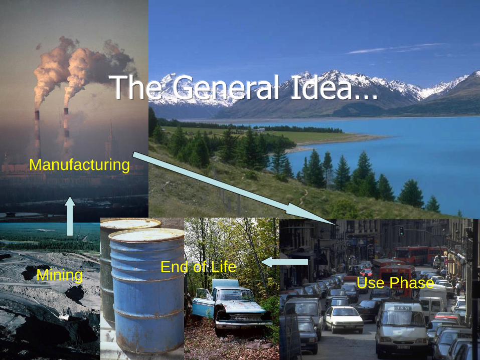
The General Idea…
Mining
Manufacturing
Use Phase End of Life
2/19/14 4
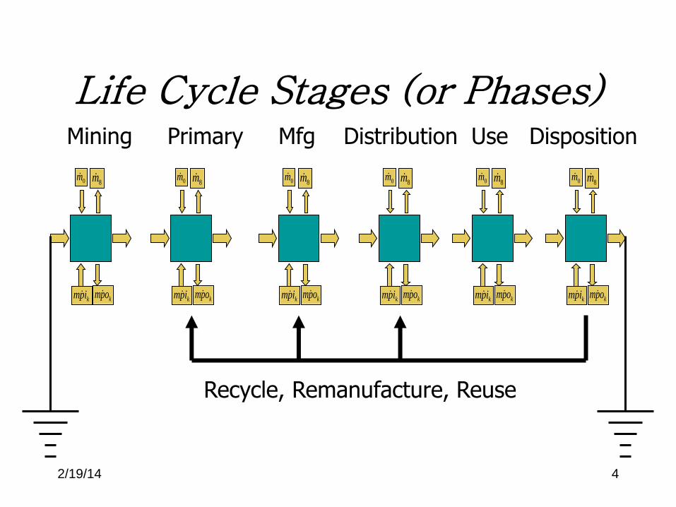
Mining Primary Mfg Distribution Use Disposition
0m8m
kipmkopm
0m8m
kipmkopm
0m8m
kipmkopm
0m8m
kipmkopm
0m8m
kipmkopm
0m8m
kipmkopm
Recycle, Remanufacture, Reuse
Life Cycle Stages (or Phases)
2/19/14 5
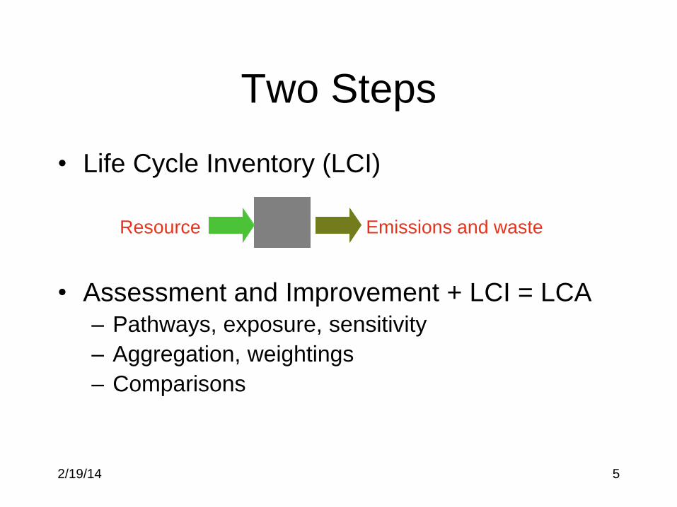
Two Steps
• Life Cycle Inventory (LCI)
Resource Emissions and waste
• Assessment and Improvement + LCI = LCA – Pathways, exposure, sensitivity
– Aggregation, weightings
– Comparisons
2/19/14 6
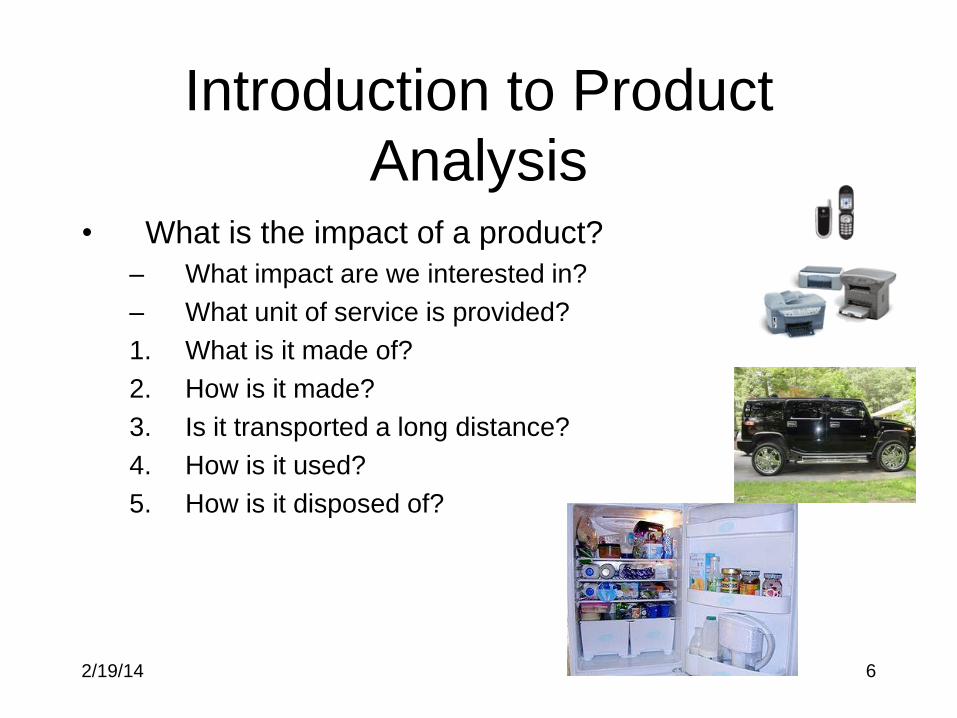
Introduction to Product
Analysis • What is the impact of a product?
– What impact are we interested in?
– What unit of service is provided?
1. What is it made of?
2. How is it made?
3. Is it transported a long distance?
4. How is it used?
5. How is it disposed of?
2/19/14 7
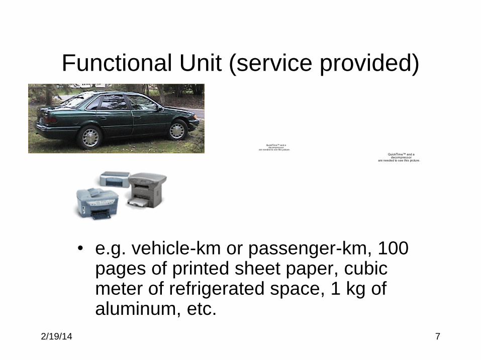
Functional Unit (service provided)
• e.g. vehicle-km or passenger-km, 100 pages of printed sheet paper, cubic meter of refrigerated space, 1 kg of aluminum, etc.
QuickTime™ and a decompressor
are needed to see this picture.
QuickTime™ and a decompressor
are needed to see this picture.
2/19/14 8
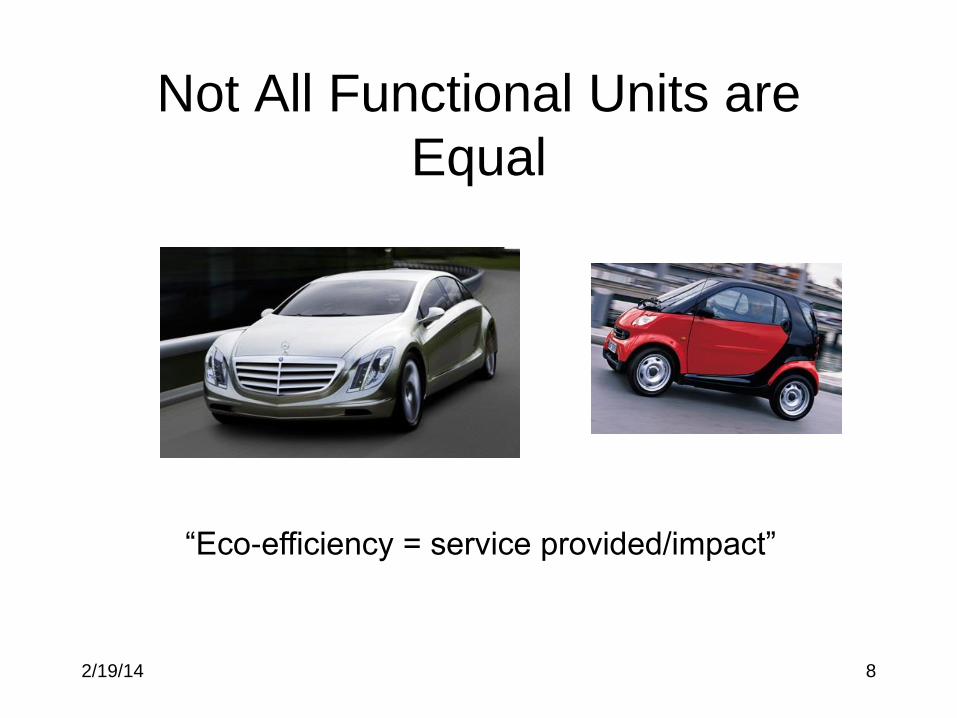
Not All Functional Units are
Equal
“Eco-efficiency = service provided/impact”
2/19/14 9
Life Cycle Perspective
1. In theory boundaries start from earth as the source, and
return to earth as the sink
2. Focus is on a product or service
3. Impact is evaluated at the receiver
4. Tracking is of materials
5. Time stands still
6. But this is hard to do, so…
2/19/14 10
Life Cycle Perspective
1. Boundaries start from earth as the source, and stop at
emissions
2. Focus is on a product or service
3. Impact potentials are aggregated (e.g.CO2e)
4. Tracking is of materials
5. Time stands still
6. We call this Life Cycle Inventory or LCI
2/19/14 11
Life Cycle Perspective
1. This can be followed by an evaluation of the
product and/or service and a redesign for
improvement
2. Typically we evaluate alternatives for comparison
3. Some of the most challenging parts include
• Identifying boundaries (what is included)
• Functional unit to represent product or service
• Allocation of impacts…who is responsible?
2/19/14 12
LCA Methods
• Streamlined Life-cycle Assessment (SLCA)
• Eco-Audit (Ashby)
• Process Models (LCI)
• Input / Output Models (EIOLCA)
2/19/14 13
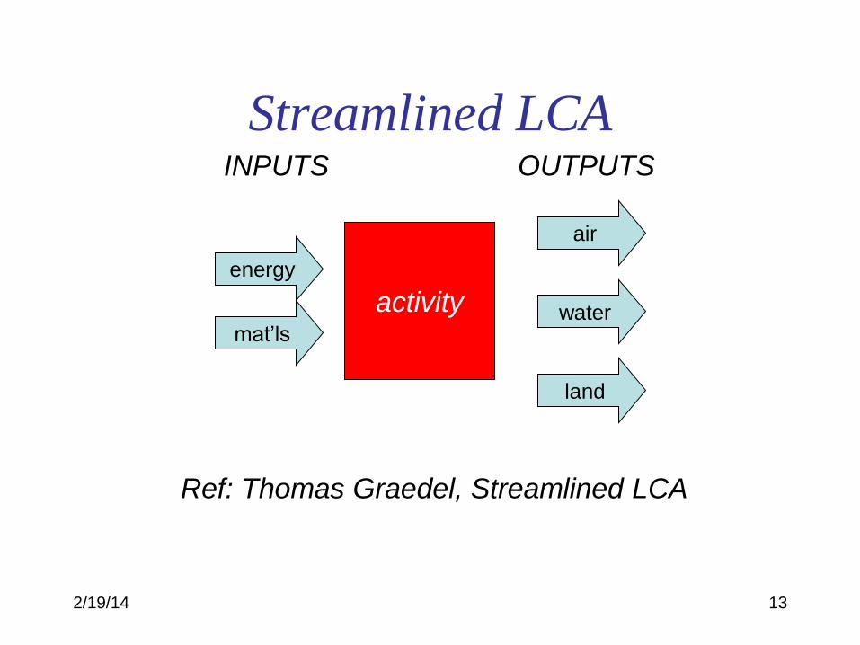
Streamlined LCA
activity
energy
mat’ls
land
water
air
INPUTS OUTPUTS
Ref: Thomas Graedel, Streamlined LCA
2/19/14 14
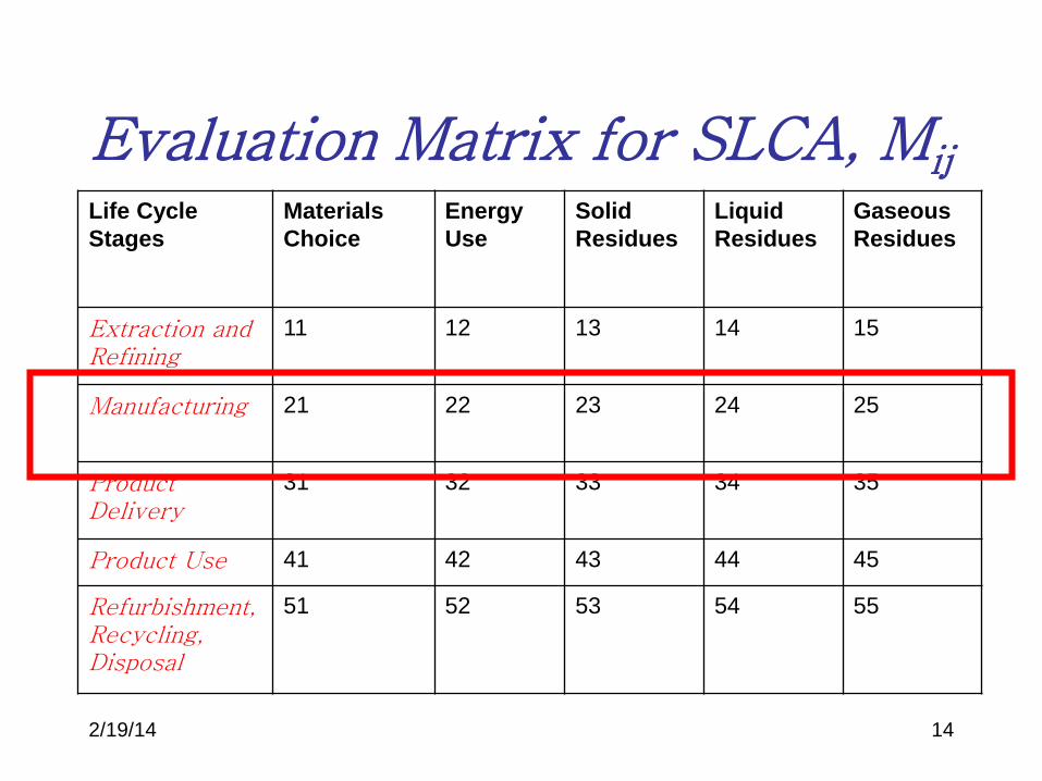
Evaluation Matrix for SLCA, Mij Life Cycle
Stages
Materials
Choice
Energy
Use
Solid
Residues
Liquid
Residues
Gaseous
Residues
Extraction and Refining
11 12 13 14 15
Manufacturing 21 22 23 24 25
Product Delivery
31 32 33 34 35
Product Use 41 42 43 44 45
Refurbishment, Recycling, Disposal
51 52 53 54 55
2/19/14 15
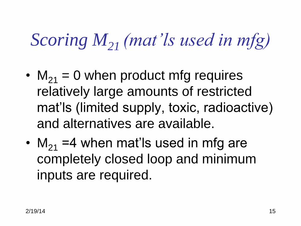
Scoring M21 (mat’ls used in mfg)
• M21 = 0 when product mfg requires
relatively large amounts of restricted
mat’ls (limited supply, toxic, radioactive)
and alternatives are available.
• M21 =4 when mat’ls used in mfg are
completely closed loop and minimum
inputs are required.
2/19/14 16
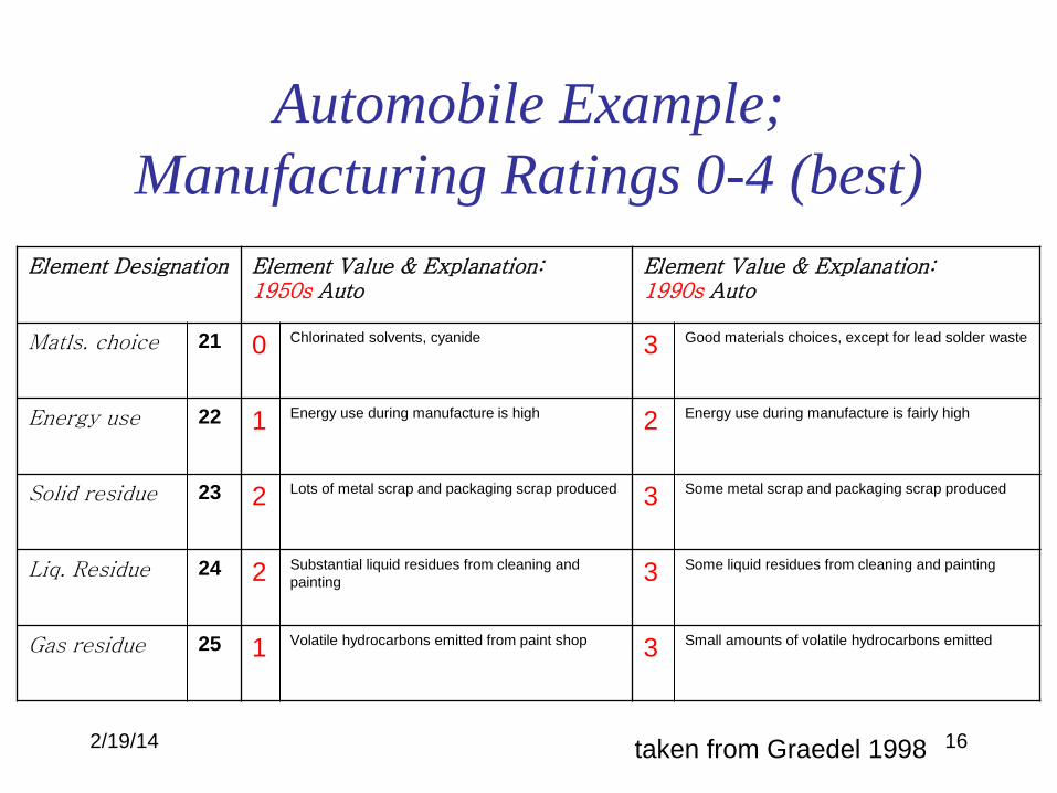
Automobile Example;
Manufacturing Ratings 0-4 (best)
Element Designation Element Value & Explanation: 1950s Auto
Element Value & Explanation: 1990s Auto
Matls. choice 21 0 Chlorinated solvents, cyanide 3 Good materials choices, except for lead solder waste
Energy use 22 1 Energy use during manufacture is high 2 Energy use during manufacture is fairly high
Solid residue 23 2 Lots of metal scrap and packaging scrap produced 3 Some metal scrap and packaging scrap produced
Liq. Residue 24 2 Substantial liquid residues from cleaning and
painting 3 Some liquid residues from cleaning and painting
Gas residue 25 1 Volatile hydrocarbons emitted from paint shop 3 Small amounts of volatile hydrocarbons emitted
taken from Graedel 1998
2/19/14 17
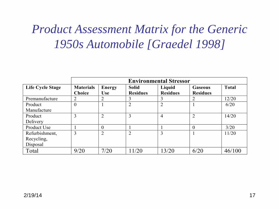
Product Assessment Matrix for the Generic
1950s Automobile [Graedel 1998]
Environmental Stressor Life Cycle Stage Materials
Choice
Energy
Use
Solid
Residues
Liquid
Residues
Gaseous
Residues
Total
Premanufacture 2 2 3 3 2 12/20
Product
Manufacture
0 1 2 2 1 6/20
Product
Delivery
3 2 3 4 2 14/20
Product Use 1 0 1 1 0 3/20
Refurbishment,
Recycling,
Disposal
3 2 2 3 1 11/20
Total 9/20 7/20 11/20 13/20 6/20 46/100
2/19/14 18
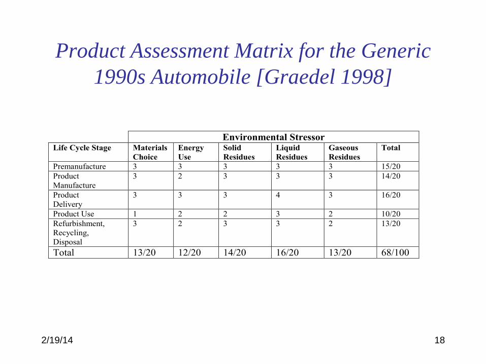
Product Assessment Matrix for the Generic
1990s Automobile [Graedel 1998]
Environmental Stressor Life Cycle Stage Materials
Choice
Energy
Use
Solid
Residues
Liquid
Residues
Gaseous
Residues
Total
Premanufacture 3 3 3 3 3 15/20
Product
Manufacture
3 2 3 3 3 14/20
Product
Delivery
3 3 3 4 3 16/20
Product Use 1 2 2 3 2 10/20
Refurbishment,
Recycling,
Disposal
3 2 3 3 2 13/20
Total 13/20 12/20 14/20 16/20 13/20 68/100
2/19/14 19
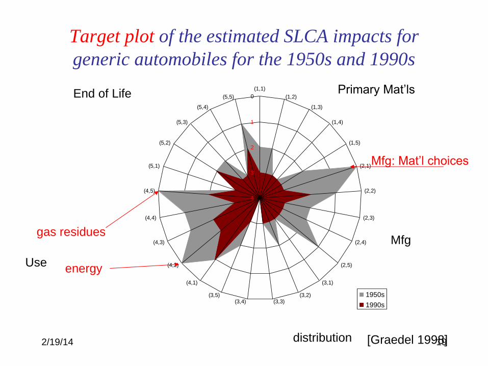
Target plot of the estimated SLCA impacts for
generic automobiles for the 1950s and 1990s
4
3
2
1
0
(1,1)
(1,2)
(1,3)
(1,4)
(1,5)
(2,1)
(2,2)
(2,3)
(2,4)
(2,5)
(3,1)
(3,2)(3,3)(3,4)
(3,5)
(4,1)
(4,2)
(4,3)
(4,4)
(4,5)
(5,1)
(5,2)
(5,3)
(5,4)
(5,5)
1950s
1990s
[Graedel 1998]
Mfg: Mat’l choices
Use
Primary Mat’ls
Mfg
distribution
End of Life
energy
gas residues
2/19/14 20
How to deal with the complexity-
• LCA software and data bases
– Hundreds of inputs and outputs
– Uniformity
– Can be non-transparent and dated
• Simplifications
– Streamlined LCA
– Fossil fuel energy and carbon
2/19/14 21
Impacts from fossil fuels
• GWP - CO2, CH4
• PM - especially from coal
• NOx - nitrogen cycle, acid rain, ground
level ozone
• SO2 - acid rain
• Hazardous chemicals- CO, VOCs, Hg,
and heavy metals
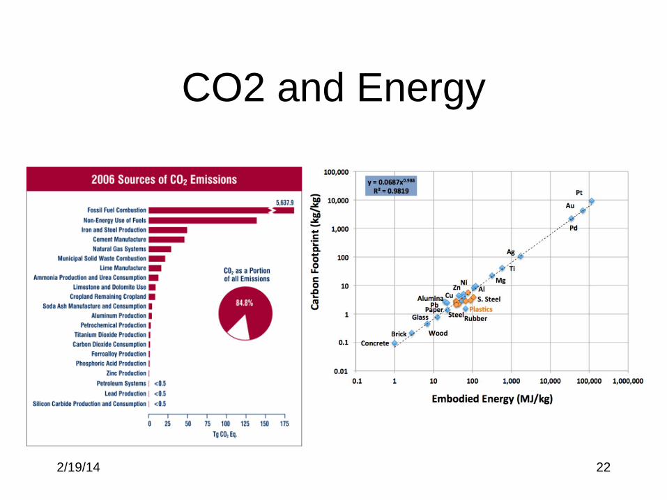
2/19/14 22
CO2 and Energy
2/19/14 23
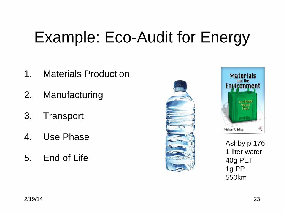
Example: Eco-Audit for Energy
1. Materials Production
2. Manufacturing
3. Transport
4. Use Phase
5. End of Life
Ashby p 176
1 liter water
40g PET
1g PP
550km
2/19/14 24
QuickTime™ and a decompressor
are needed to see this picture.
Ashby 2009
Materials
2/19/14 25
QuickTime™ and a decompressor
are needed to see this picture.
Manufacturing
Injection molding:
3MJ/kg x 2 x 3 =
~ 18 to 20 MJ/kg
Includes
•Extrusion
•Grid Losses
•Runners and
startup losses
Gutowski
“Ch 6” TDR
or Ashby
p 133-135, 154
2/19/14 26
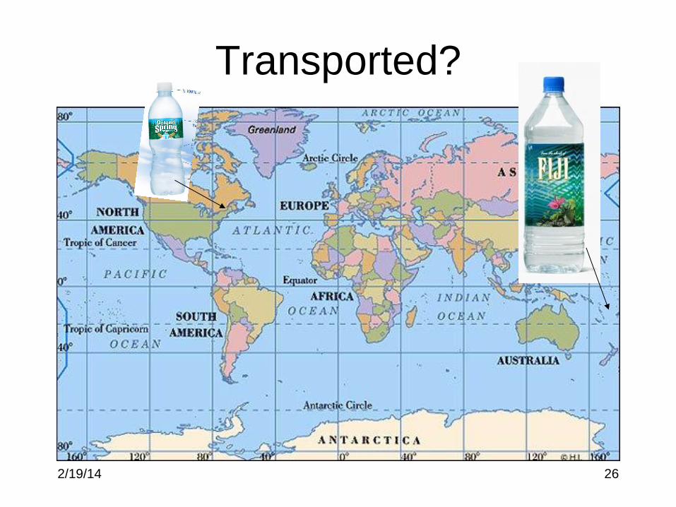
Transported?
2/19/14 27
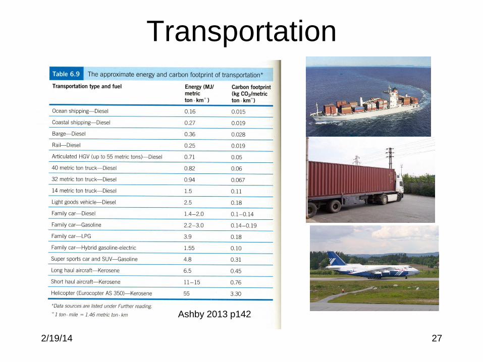
Transportation
Ashby 2013 p142
2/19/14 28
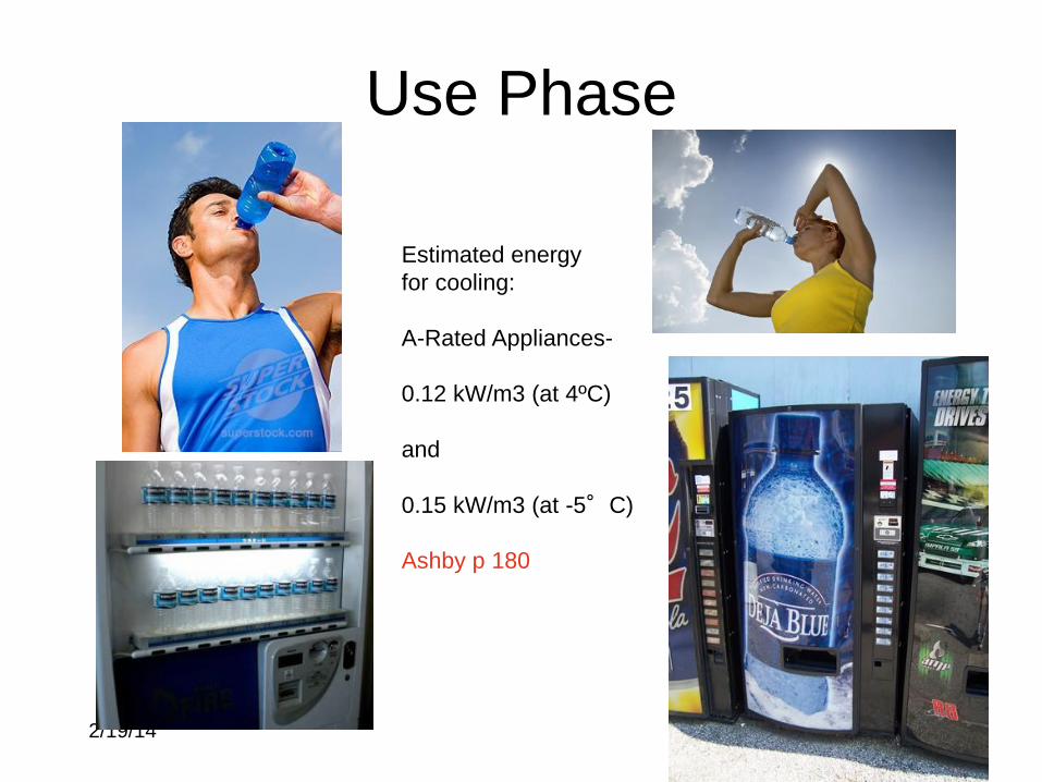
Use Phase
Estimated energy
for cooling:
A-Rated Appliances-
0.12 kW/m3 (at 4ºC)
and
0.15 kW/m3 (at -5°C)
Ashby p 180
2/19/14 29
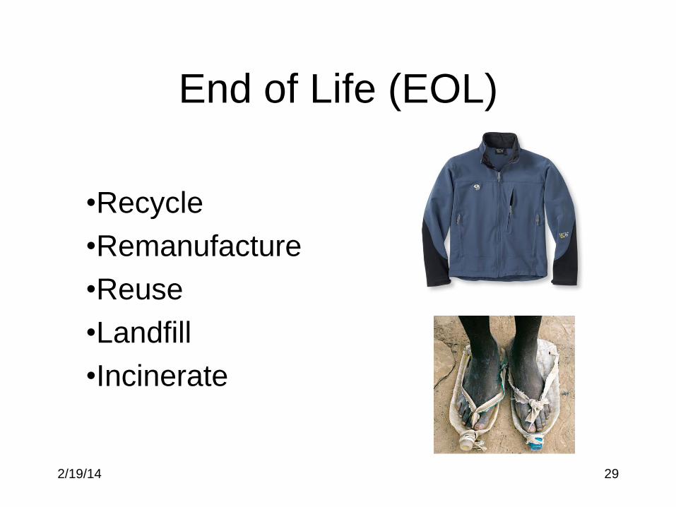
End of Life (EOL)
•Recycle
•Remanufacture
•Reuse
•Landfill
•Incinerate
2/19/14 30
QuickTime™ and a decompressor
are needed to see this picture.
Ashby 2009
Recycling rates as fraction of supply
2/19/14 31
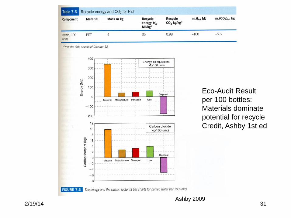
Eco-Audit Result
per 100 bottles:
Materials dominate
potential for recycle
Credit, Ashby 1st ed
Ashby 2009
2/19/14 32
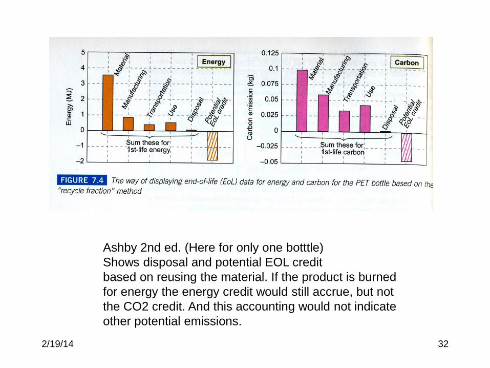
Ashby 2nd ed. (Here for only one botttle)
Shows disposal and potential EOL credit
based on reusing the material. If the product is burned
for energy the energy credit would still accrue, but not
the CO2 credit. And this accounting would not indicate
other potential emissions.
2/19/14 33
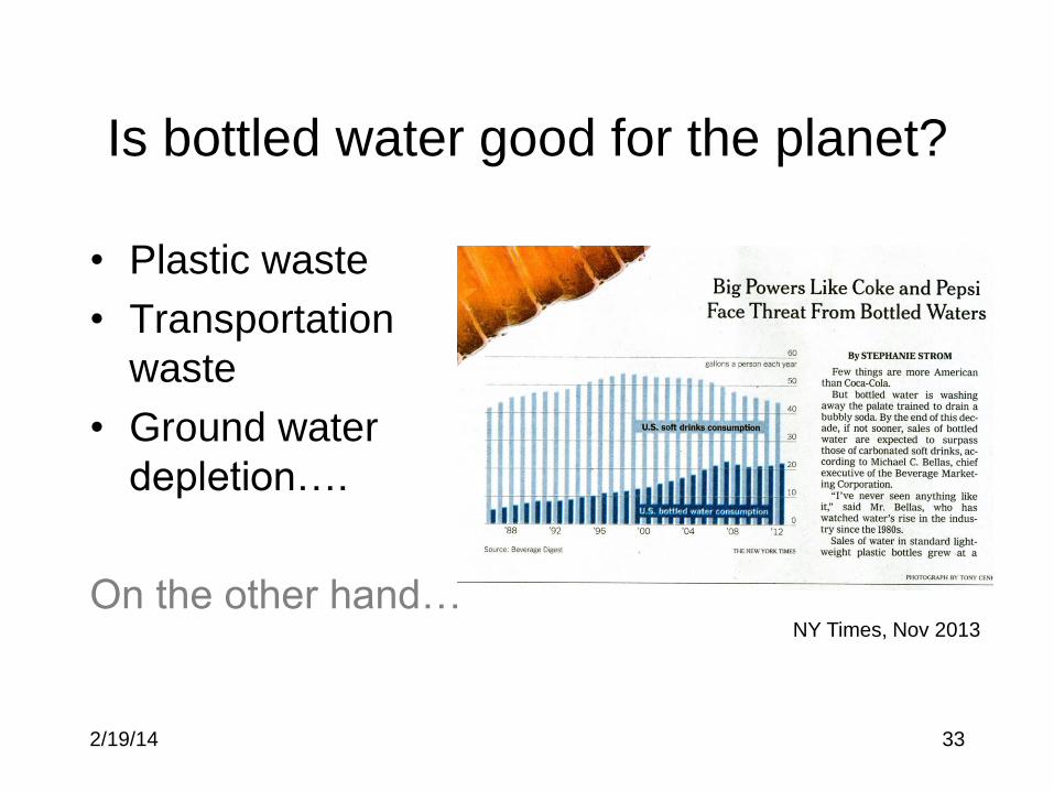
Is bottled water good for the planet?
• Plastic waste
• Transportation
waste
• Ground water
depletion….
On the other hand… NY Times, Nov 2013
2/19/14 34
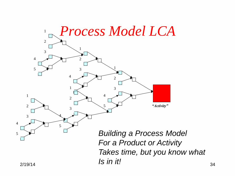
Process Model LCA
“Activity”
1
2
3
4
5
1
2
3
4
5
1
2
3
4
5
1
2
3
4
5
1
2
3
4
5 Building a Process Model
For a Product or Activity
Takes time, but you know what
Is in it!
2/19/14 35
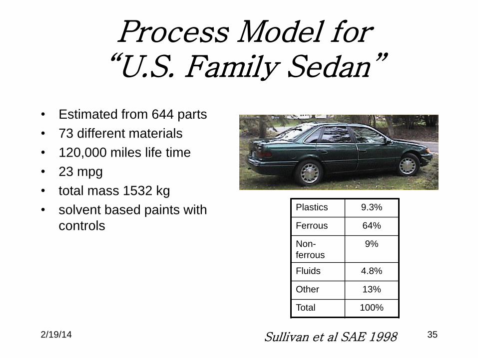
Process Model for “U.S. Family Sedan”
• Estimated from 644 parts
• 73 different materials
• 120,000 miles life time
• 23 mpg
• total mass 1532 kg
• solvent based paints with
controls
Sullivan et al SAE 1998
Plastics 9.3%
Ferrous 64%
Non-
ferrous
9%
Fluids 4.8%
Other 13%
Total 100%
2/19/14 36
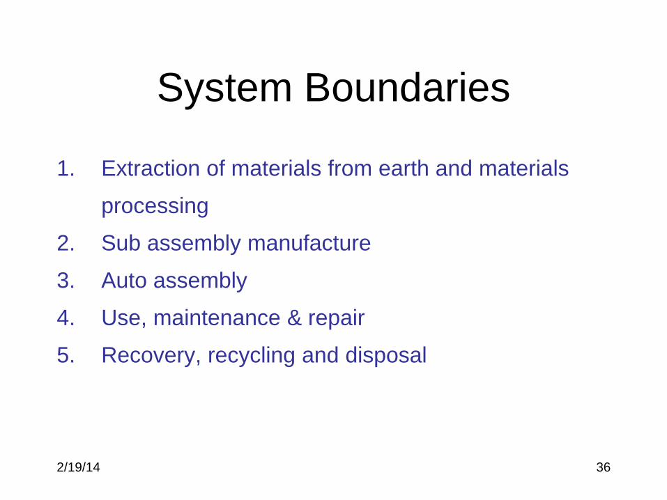
System Boundaries
1. Extraction of materials from earth and materials
processing
2. Sub assembly manufacture
3. Auto assembly
4. Use, maintenance & repair
5. Recovery, recycling and disposal
2/19/14 37
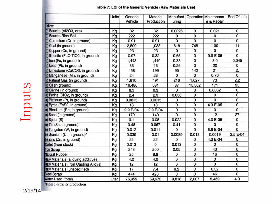
Inputs
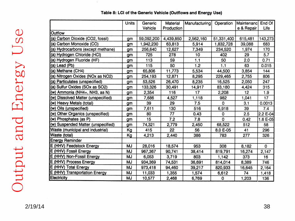
2/19/14 38
Outp
ut
and E
nerg
y U
se
2/19/14 39
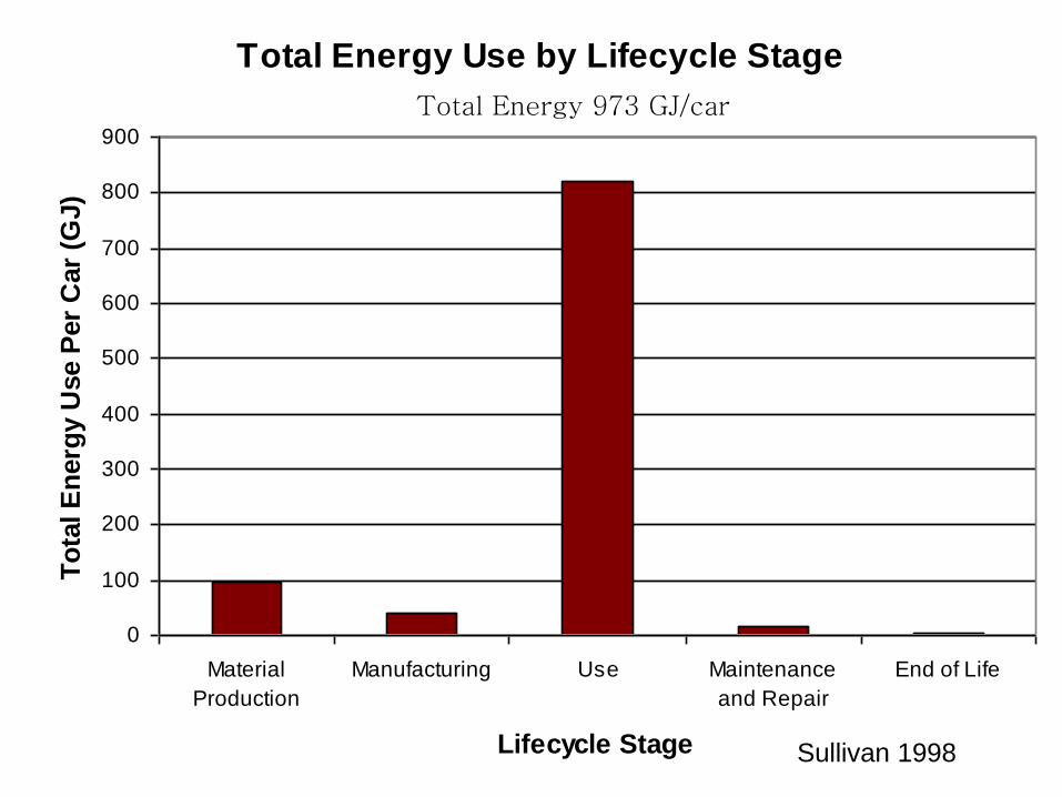
Total Energy Use by Lifecycle Stage
0
100
200
300
400
500
600
700
800
900
Material
Production
Manufacturing Use Maintenance
and Repair
End of Life
Lifecycle Stage
To
tal E
nerg
y U
se P
er
Car
(GJ)
Sullivan 1998
Total Energy 973 GJ/car
2/19/14 40
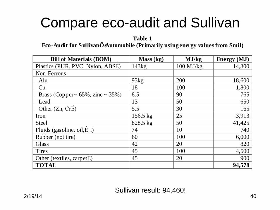
Table 1
Eco-Audit for SullivanÕs Automobile (Primarily using energy values from Smil)
Bill of Materials (BOM) Mass (kg) MJ/kg Energy (MJ)
Plastics (PUR, PVC, Nylon, ABSÉ) 143kg 100 MJ/kg 14,300
Non-Ferrous
Alu 93kg 200 18,600
Cu 18 100 1,800
Brass (Copper ~ 65%, zinc ~ 35%) 8.5 90 765
Lead 13 50 650
Other (Zn, CrÉ) 5.5 30 165
Iron 156.5 kg 25 3,913
Steel 828.5 kg 50 41,425
Fluids (gasoline, oil,É .) 74 10 740
Rubber (not tire) 60 100 6,000
Glass 42 20 820
Tires 45 100 4,500
Other (textiles, carpetÉ) 45 20 900
TOTAL 94,578
Sullivan result: 94,460!
Compare eco-audit and Sullivan
2/19/14 41
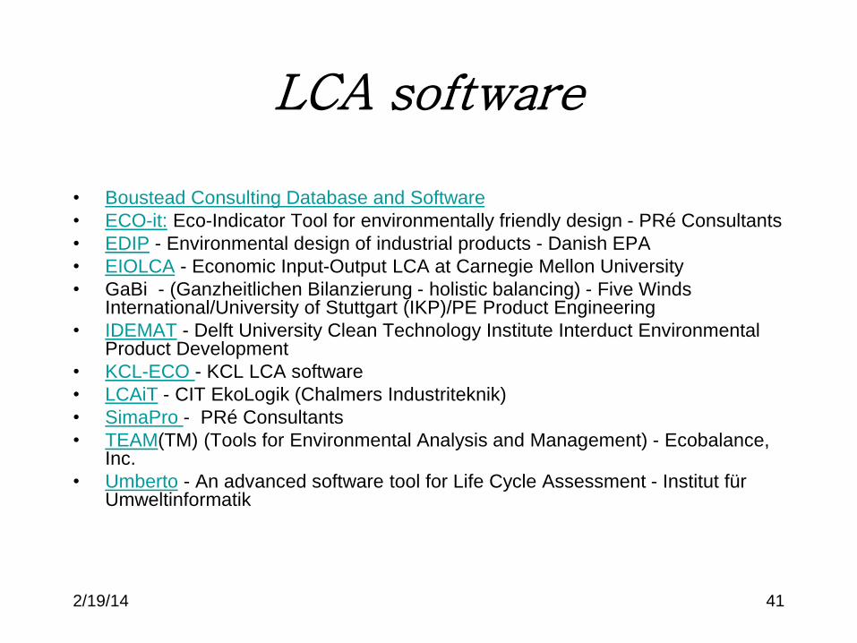
LCA software
• Boustead Consulting Database and Software
• ECO-it: Eco-Indicator Tool for environmentally friendly design - PRé Consultants
• EDIP - Environmental design of industrial products - Danish EPA
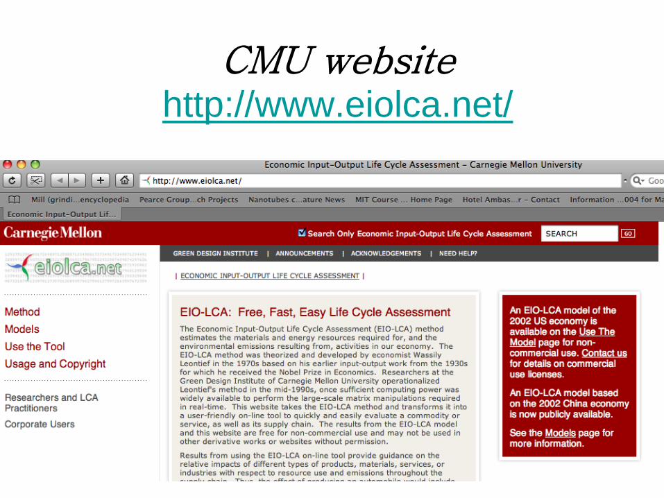
• EIOLCA - Economic Input-Output LCA at Carnegie Mellon University
• GaBi - (Ganzheitlichen Bilanzierung - holistic balancing) - Five Winds International/University of Stuttgart (IKP)/PE Product Engineering
• IDEMAT - Delft University Clean Technology Institute Interduct Environmental Product Development
• KCL-ECO - KCL LCA software
• LCAiT - CIT EkoLogik (Chalmers Industriteknik)
• SimaPro - PRé Consultants
• TEAM(TM) (Tools for Environmental Analysis and Management) - Ecobalance, Inc.
• Umberto - An advanced software tool for Life Cycle Assessment - Institut für Umweltinformatik
2/19/14 42
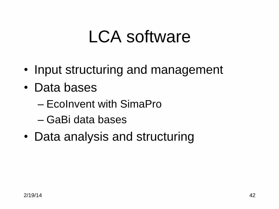
LCA software
• Input structuring and management
• Data bases
– EcoInvent with SimaPro
– GaBi data bases
• Data analysis and structuring
2/19/14 43
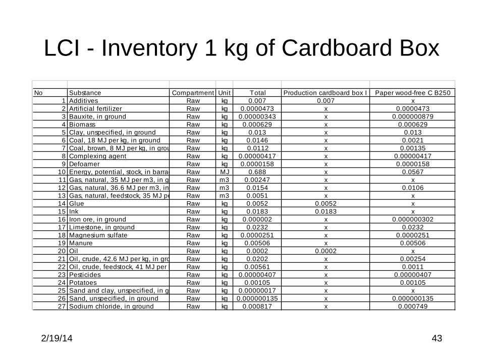
LCI - Inventory 1 kg of Cardboard Box
No Substance Compartment Unit Total Production cardboard box I Paper wood-free C B250
1 Additives Raw kg 0.007 0.007 x
2 Artificial ferti l izer Raw kg 0.0000473 x 0.0000473
3 Bauxite, in ground Raw kg 0.00000343 x 0.000000879
4 Biomass Raw kg 0.000629 x 0.000629
5 Clay, unspecified, in ground Raw kg 0.013 x 0.013
6 Coal, 18 MJ per kg, in ground Raw kg 0.0146 x 0.0021
7 Coal, brown, 8 MJ per kg, in ground Raw kg 0.0112 x 0.00135
8 Complexing agent Raw kg 0.00000417 x 0.00000417
9 Defoamer Raw kg 0.0000158 x 0.0000158
10 Energy, potential, stock, in barrage waterRaw MJ 0.688 x 0.0567
11 Gas, natural, 35 MJ per m3, in groundRaw m3 0.00247 x x
12 Gas, natural, 36.6 MJ per m3, in groundRaw m3 0.0154 x 0.0106
13 Gas, natural, feedstock, 35 MJ per m3, in groundRaw m3 0.0051 x x
14 Glue Raw kg 0.0052 0.0052 x
15 Ink Raw kg 0.0183 0.0183 x
16 Iron ore, in ground Raw kg 0.000002 x 0.000000302
17 Limestone, in ground Raw kg 0.0232 x 0.0232
18 Magnesium sulfate Raw kg 0.0000251 x 0.0000251
19 Manure Raw kg 0.00506 x 0.00506
20 Oil Raw kg 0.0002 0.0002 x
21 Oil, crude, 42.6 MJ per kg, in ground Raw kg 0.0202 x 0.00254
22 Oil, crude, feedstock, 41 MJ per kg, in groundRaw kg 0.00561 x 0.0011
23 Pesticides Raw kg 0.00000407 x 0.00000407
24 Potatoes Raw kg 0.00105 x 0.00105
25 Sand and clay, unspecified, in groundRaw kg 0.00000017 x x
26 Sand, unspecified, in ground Raw kg 0.000000135 x 0.000000135
27 Sodium chloride, in ground Raw kg 0.000817 x 0.000749
2/19/14 44
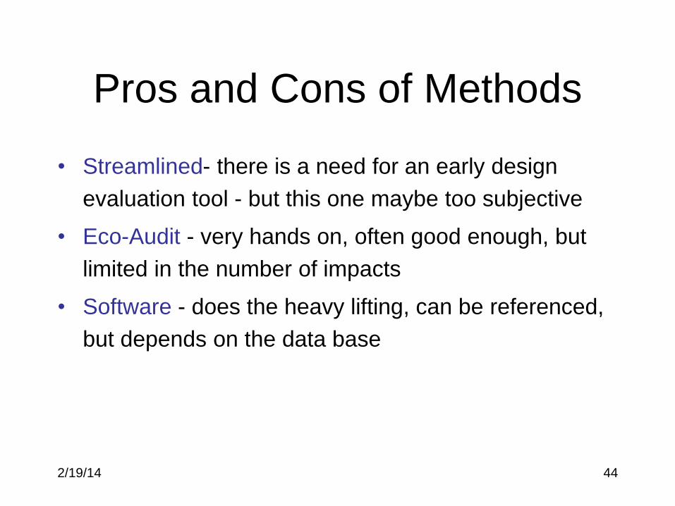
Pros and Cons of Methods
• Streamlined- there is a need for an early design
evaluation tool - but this one maybe too subjective
• Eco-Audit - very hands on, often good enough, but
limited in the number of impacts
• Software - does the heavy lifting, can be referenced,
but depends on the data base
2/19/14 45
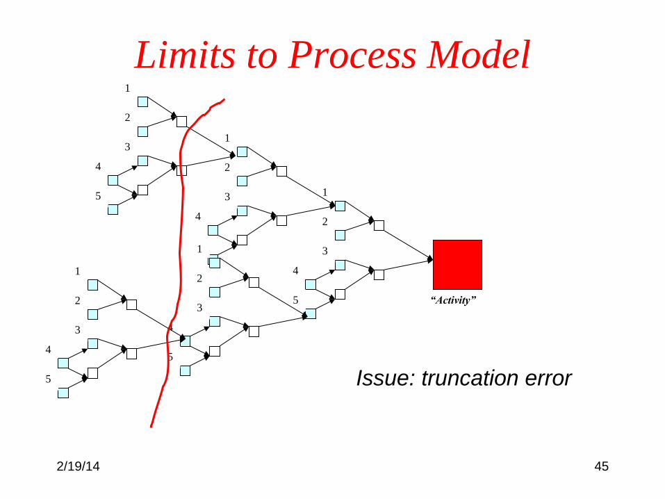
Limits to Process Model
“Activity”
1
2
3
4
5
1
2
3
4
5
1
2
3
4
5
1
2
3
4
5
1
2
3
4
5 Issue: truncation error
2/19/14 46
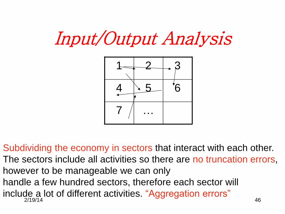
Input/Output Analysis
1 2 3
4 5 6
7 …
Subdividing the economy in sectors that interact with each other.
The sectors include all activities so there are no truncation errors,
however to be manageable we can only
handle a few hundred sectors, therefore each sector will
include a lot of different activities. “Aggregation errors”
2/19/14 47
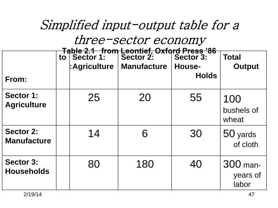
Simplified input-output table for a three-sector economy
Table 2.1 from Leontief, Oxford Press ’86
From:
to
:
Sector 1:
Agriculture
Sector 2:
Manufacture
Sector 3:
House-
Holds
Total
Output
Sector 1:
Agriculture
25 20 55 100 bushels of
wheat
Sector 2:
Manufacture
14 6 30 50 yards
of cloth
Sector 3:
Households 80 180 40 300 man-
years of
labor
2/19/14 48
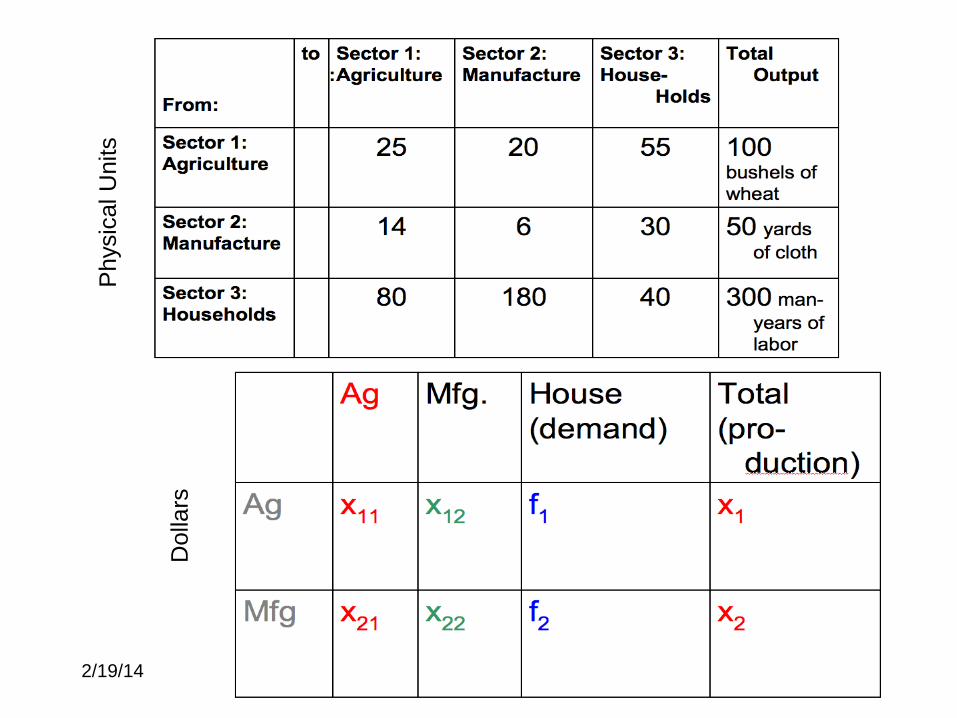
Physic
al U
nits
Dolla
rs
2/19/14 49
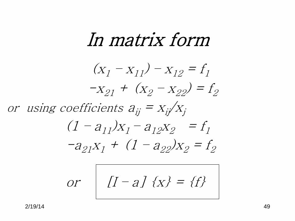
In matrix form
(x1 – x11) – x12 = f1
-x21 + (x2 – x22) = f2
or using coefficients aij = xij/xj
(1 – a11)x1 – a12x2 = f1
-a21x1 + (1 – a22)x2 = f2
or [I – a] {x} = {f}
2/19/14 50
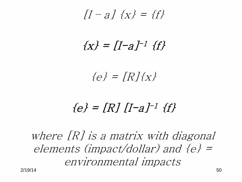
where [R] is a matrix with diagonal elements (impact/dollar) and {e} =
environmental impacts
[I – a] {x} = {f}
{x} = [I-a]-1 {f}
{e} = [R]{x}
{e} = [R] [I-a]-1 {f}
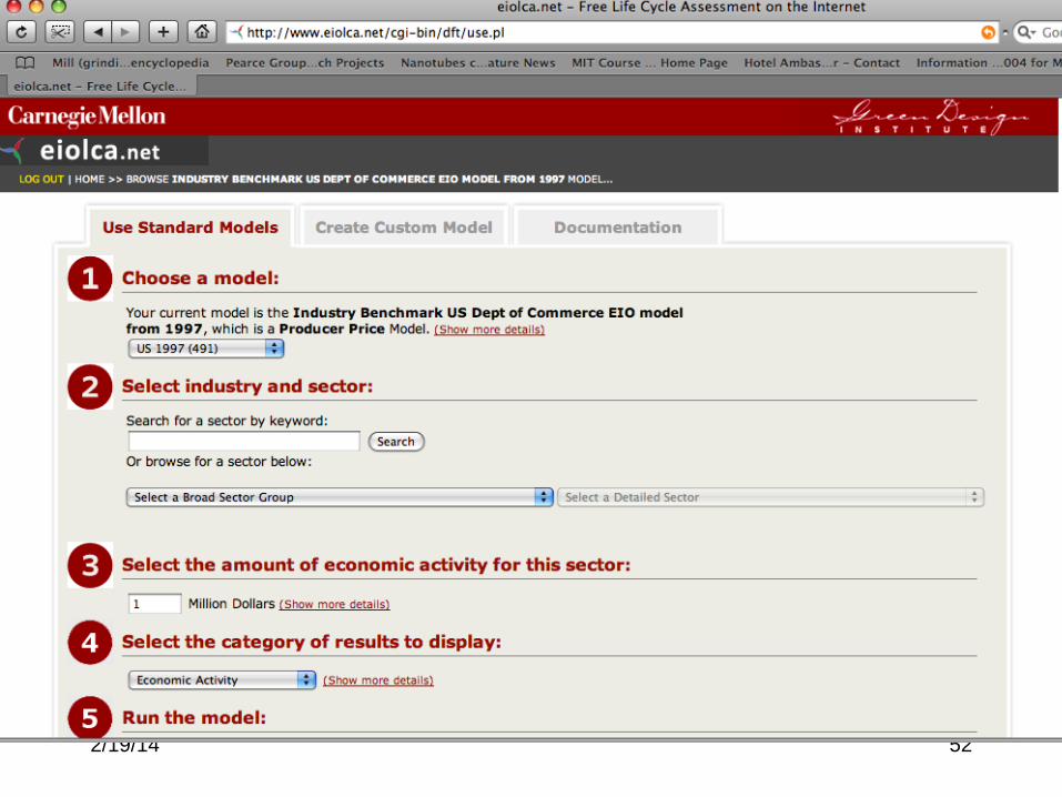
2/19/14 52
2/19/14 53
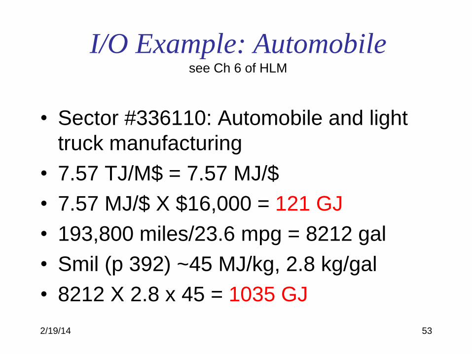
I/O Example: Automobile see Ch 6 of HLM
• Sector #336110: Automobile and light
truck manufacturing
• 7.57 TJ/M$ = 7.57 MJ/$
• 7.57 MJ/$ X $16,000 = 121 GJ
• 193,800 miles/23.6 mpg = 8212 gal
• Smil (p 392) ~45 MJ/kg, 2.8 kg/gal
• 8212 X 2.8 x 45 = 1035 GJ
2/19/14 54
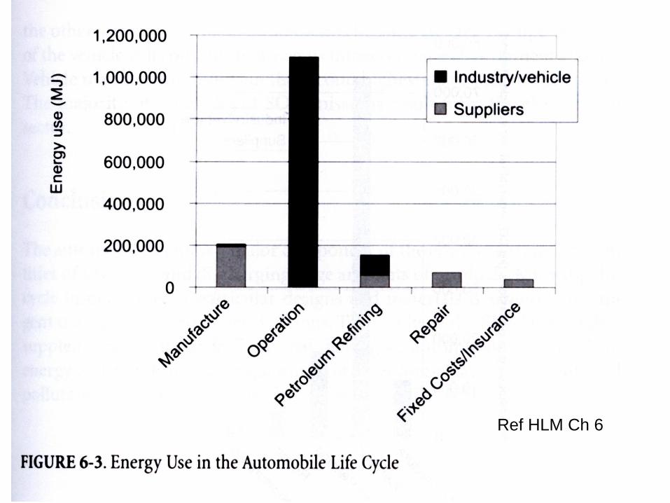
Ref HLM Ch 6
2/19/14 55
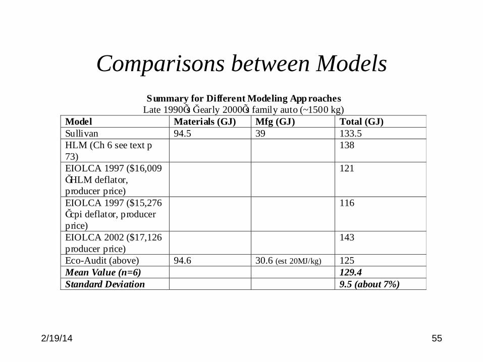
Summary for Different Modeling App roaches
Late 1990Õs Ğ early 2000Õs family auto (~1500 kg)
Model Materials (GJ) Mfg (GJ) Total (GJ)
Sullivan 94.5 39 133.5
HLM (Ch 6 see text p
73)
138
EIOLCA 1997 ($16,009
ĞHLM deflator,
producer price)
121
EIOLCA 1997 ($15,276
Ğcpi deflator, producer
price)
116
EIOLCA 2002 ($17,126
producer price)
143
Eco-Audit (above) 94.6 30.6 (est 20MJ/kg) 125
Mean Value (n=6) 129.4
Standard Deviation 9.5 (about 7%)
Comparisons between Models
2/19/14 56
Issues with EIOLCA
• Builds on economic data
• Economy wide effects
• Highly aggregated
• Time delay
• Normalized by economic activity (e.g. MJ/$)
• Trouble with foreign trade
• Very powerful (“requires professional
supervision”)
2/19/14 57
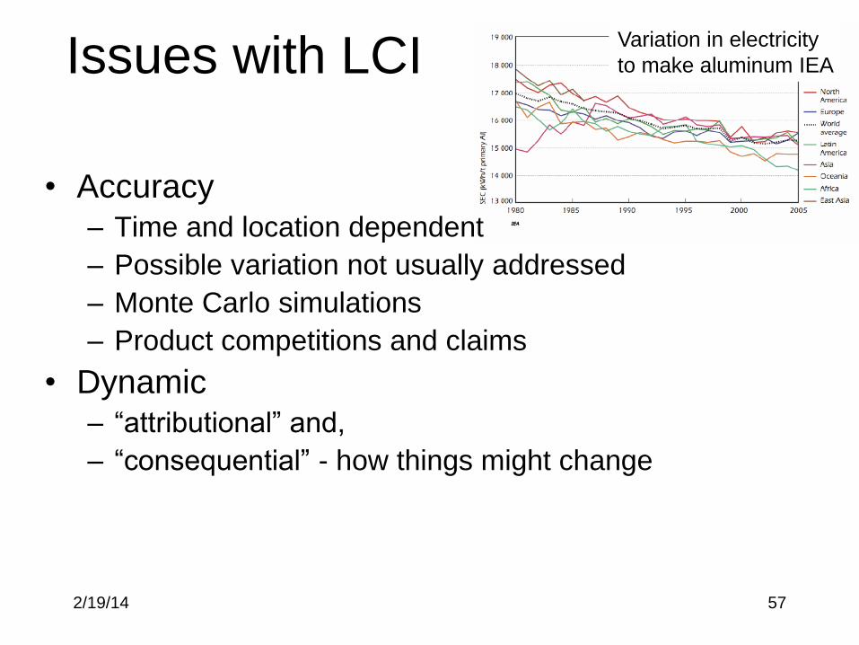
Issues with LCI
• Accuracy – Time and location dependent
– Possible variation not usually addressed
– Monte Carlo simulations
– Product competitions and claims
• Dynamic – “attributional” and,
– “consequential” - how things might change
Variation in electricity
to make aluminum IEA
2/19/14 58
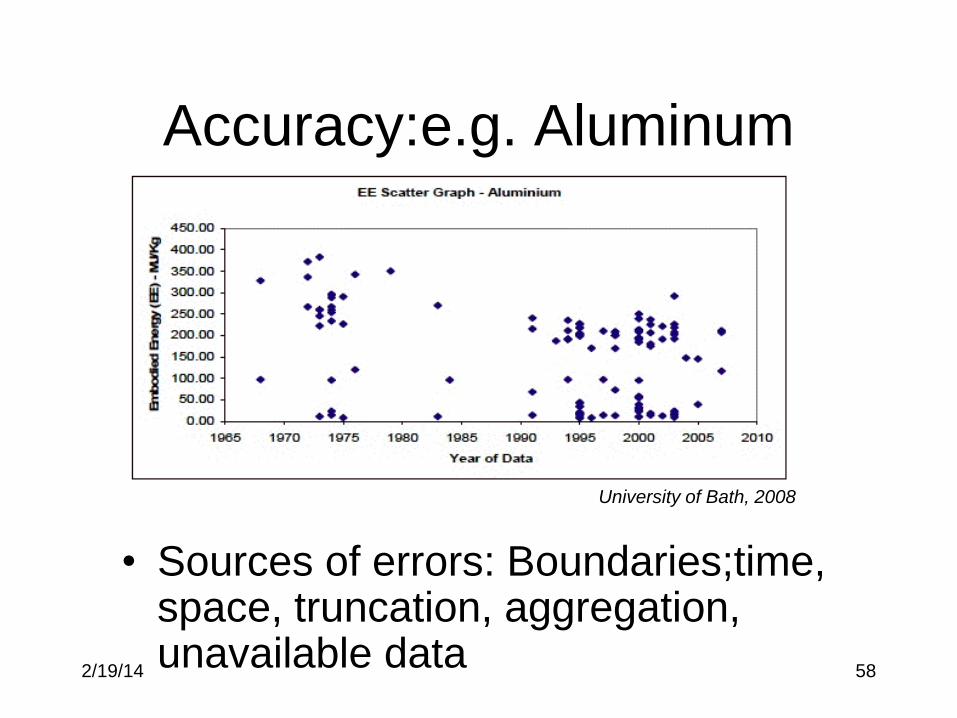
Accuracy:e.g. Aluminum
• Sources of errors: Boundaries;time, space, truncation, aggregation, unavailable data
University of Bath, 2008
2/19/14 59
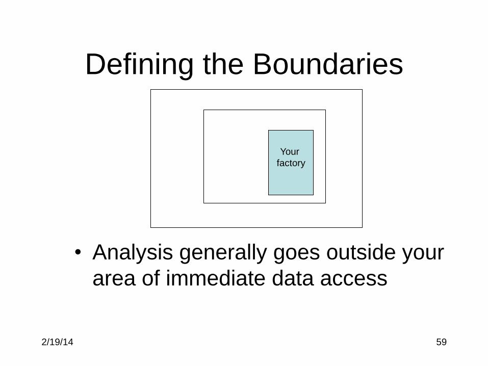
Defining the Boundaries
• Analysis generally goes outside your
area of immediate data access
Your
factory
2/19/14 60
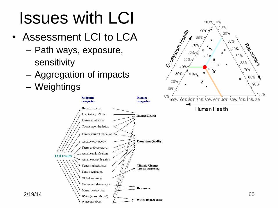
Issues with LCI • Assessment LCI to LCA
– Path ways, exposure,
sensitivity
– Aggregation of impacts
– Weightings
2/19/14 61
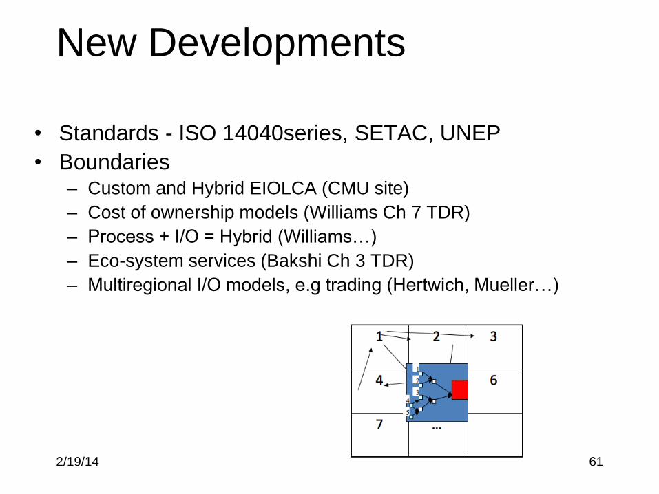
New Developments
• Standards - ISO 14040series, SETAC, UNEP
• Boundaries – Custom and Hybrid EIOLCA (CMU site)
– Cost of ownership models (Williams Ch 7 TDR)
– Process + I/O = Hybrid (Williams…)
– Eco-system services (Bakshi Ch 3 TDR)
– Multiregional I/O models, e.g trading (Hertwich, Mueller…)
2/19/14 62
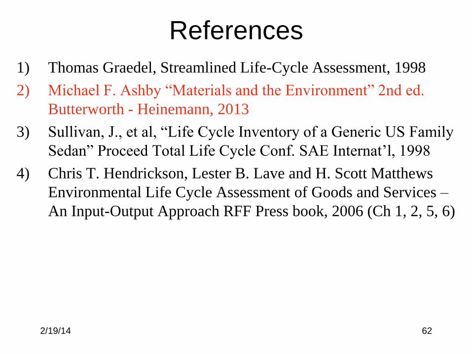
References
1) Thomas Graedel, Streamlined Life-Cycle Assessment, 1998
2) Michael F. Ashby “Materials and the Environment” 2nd ed.
Butterworth - Heinemann, 2013
3) Sullivan, J., et al, “Life Cycle Inventory of a Generic US Family
Sedan” Proceed Total Life Cycle Conf. SAE Internat’l, 1998
4) Chris T. Hendrickson, Lester B. Lave and H. Scott Matthews
Environmental Life Cycle Assessment of Goods and Services –
An Input-Output Approach RFF Press book, 2006 (Ch 1, 2, 5, 6)