Nau: Game Theory 1

Introduction to Game Theory

9. Incomplete-Information Games

Dana Nau University of Maryland

Nau: Game Theory 2

Introduction   All the kinds of games we’ve looked at so far have assumed that

  everything relevant about the game being played is common knowledge to all the players:

  the number of players,   the actions available to each , and   the payoff vector associated with each action vector

  True even for imperfect-information games   The actual moves aren’t common knowledge, but the game is

  We’ll now consider games of incomplete (not imperfect) information   Players are uncertain about the game being played

Nau: Game Theory 3

Example   Consider the payoff matrix shown here

ε is a small positive constant   Agent 2’s payoffs are arbitrary constants a, b, c, d.

  Thus the matrix represents a set of games   Agent 1 doesn’t know which of these games

is the one he/she is playing   Agent 1 wants a strategy that makes sense despite this lack of

knowledge   Agent 1 might want to play a maximin, or “safety level,” strategy

  Agent 2’s minimax strategy is to play R, and B is a best response to R.   So agent 1’s maximin strategy is to play B

Nau: Game Theory 4

Regret   But, if agent 1 doesn’t believe that agent 2

is malicious, he/she might reason as follows   Suppose agent 2 plays R

•  Agent 1’s payoff is either 1 or 1–ε •  Thus agent 1’s strategy doesn’t change

his/her payoff much: ›  Difference is only ε

  Suppose agent 2 plays L, •  Agent 1’s payoff is either 100 or 2 •  In this case, agent 1’s action matters much more

›  Difference in agent 1’s payoff is 98   So agent 1 might choose T to minimize his/her worst-case loss

  This is the opposite of agent 1’s maximin strategy

Nau: Game Theory 5

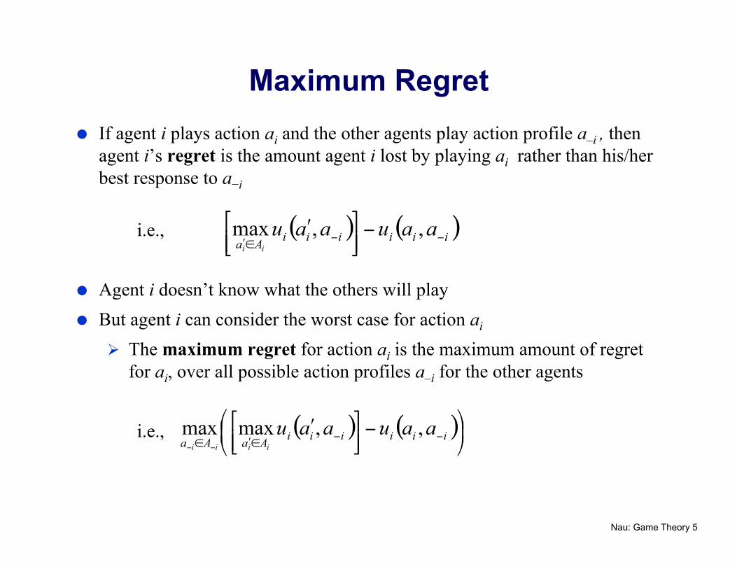
Maximum Regret   If agent i plays action ai and the other agents play action profile a–i , then

agent i’s regret is the amount agent i lost by playing ai rather than his/her best response to a−i

i.e.,

  Agent i doesn’t know what the others will play   But agent i can consider the worst case for action ai

  The maximum regret for action ai is the maximum amount of regret for ai, over all possible action profiles a–i for the other agents

i.e.,

Nau: Game Theory 6

Minimax Regret   Finally, agent i can choose his/her action to minimize this worst-case regret

  An agent’s minimax regret action is an action giving the smallest maximum regret, i.e.,

  Minimax regret can be extended to a solution concept in the natural way   Identify action profiles that consist of minimax regret actions for each

agent €

argminai ∈Ai

maxa− i ∈A− i

maxʹ′ a i ∈Ai

ui ʹ′ a i,a−i( )⎡ ⎣ ⎢

⎤ ⎦ ⎥ − ui ai,a−i( )

⎛

⎝ ⎜

⎞

⎠ ⎟

⎛

⎝ ⎜

⎞

⎠ ⎟

Nau: Game Theory 7

Bayesian Games   In the previous example, we knew the set G of all possible games, but

didn’t know which game in G   Suppose we have enough information to put a probability distribution

over the games   A Bayesian Game is a class of games G that satisfies two fundamental

conditions   Condition 1:

  The games in G have the same number of agents, and the same strategy space for each agent. The only difference is in the payoffs of the strategies.

  This condition isn’t very restrictive   Other types of uncertainty can be reduced to the above, by

reformulating the problem

Nau: Game Theory 8

Example   Suppose we don’t know whether player 2 only has strategies L and R, or also an

additional strategy C:

Game G1 Game G2

  If player 2 doesn’t have strategy C, this is equivalent to having a strategy C that’s dominated by the other strategies:

•  Game G1'

  The Nash equilibria for G1' are the same as the Nash equilibria for G1

  We’ve reduced the problem to whether C’s payoffs are those of G1' or G2

Nau: Game Theory 9

Bayesian Games   Condition 2 (common prior): the probability distribution over the games in

G is common knowledge (i.e., known to all the agents)   So a Bayesian game defines

  the uncertainties of agents about the game being played,   what each agent believes the other agents believe about the game being

played   The beliefs of the different agents are posterior probabilities

  Got by conditioning the common prior on individual “private signals” (what’s “revealed” to the individual players)

  The common-prior assumption rules out whole families of games   But it greatly simplifies the theory

  Hence most work in game theory uses it

Nau: Game Theory 10

Bayes-Nash Equilibria   The concept of a Nash equilibrium can be extended to Bayesian games

  Bayes-Nash equilibrium   The details are complicated, and I’ll skip them

  But I’ll give you some examples

Nau: Game Theory 11

Example: Auctions   An auction is a way (other than bargaining) to sell a fixed supply of a

commodity (an item to be sold) for which there is no well-established ongoing market

  Bidders make bids   proposals to pay various amounts of money for the commodity

  The commodity is sold to the bidder who makes the largest bid   Example applications

  Real estate, art, oil leases, electromagnetic spectrum, electricity, eBay, google ads

  Several kinds of auctions are incomplete-information, and can be modeled as Bayesian games

Nau: Game Theory 12

Types of Auctions   Classification according to how the commodity is valued:

  Private value auctions •  Each bidder may have a different bidder value (BV), i.e., how much the

commodity is worth to that bidder •  A bidder’s BV is his/her private information, not known to others

•  E.g., flowers, art, antiques

  Common-value auctions •  The ultimate value of the item is the same for all bidders, but bidders are

unsure what that ultimate value is •  E.g., oil leases, Olympic broadcast rights

  Affiliated (correlated) value auctions

•  These are somewhere between private and common-value auctions •  BVs for the auctioned item(s) are correlated, but not necessarily the same

for all

Nau: Game Theory 13

Types of Auctions   Classification according to the rules for bidding

•  English •  Dutch

•  First price sealed bid •  Vickrey

•  many others

  On the following pages, I’ll describe several of these and will analyze their equilibria

  A possible problem is collusion (secret agreements for fraudulent purposes)

  Groups of bidders who won’t bid against each other, to keep the price low   Bidders who place phony (phantom) bids to raise the price (hence the

auctioneer’s profit)

  If there’s collusion, the equilibrium analysis is no longer valid

Nau: Game Theory 14

English Auction   The name comes from oral auctions in English-speaking countries

  But I think this kind of auction was also used in ancient Rome   Commodities:

  antiques, artworks, cattle, horses, real estate, wholesale fruits and vegetables, old books, etc.

  Typical rules:

  Auctioneer first solicits an opening bid from the group   Anyone who wants to bid should call out a new price at least x higher than the

previous high bid (e.g., x = 1 Euro)   The bidding continues until all bidders but one have dropped out

  The highest bidder gets the object being sold, for a price equal to the final bid

  Winner’s profit = BV – price   Everyone else’s profit = 0

Nau: Game Theory 15

English Auction (continued)   Optimal strategy:

  participate until highest bid = your valuation of the commodity, then drop out

  Equilibrium Outcome   The highest bidder gets the object, at a price close to the second highest

BV   Let n be the number of bidders

  The higher n is, the closer winning bid is to the highest BV.   If there is a large range of BVs, then the difference between the highest

and 2nd-highest BVs may be large •  Thus if there’s wide disagreement about the item’s value, the

winner might be able to get it for much less than his/her BV

Nau: Game Theory 16

Let’s Do an English Auction   I will auction one Euro in an English auction

  The Euro will be sold to the highest bidder, for the amount of his/her bid

  Do not collude   The minimum increment for a new bid is 5 cents

Nau: Game Theory 17

Let’s Do Another Auction   This auction is like the first, but with one more rule

  The Euro will be sold to the highest bidder, for the amount of his/her bid

  The second highest bidder must also pay his/her bid, but receives nothing

  Do not collude   The minimum increment for a new bid is 5 cents

Nau: Game Theory 18

First-Price Sealed-Bid Auctions   Examples:

  construction contracts (lowest bidder)   real estate   art treasures

  Typical rules   Bidders write their bids for the object and their names on slips of

paper and deliver them to the auctioneer   The auctioneer opens the bid and finds the highest bidder   The highest bidder gets the object being sold, for a price equal to

his/her own bid   Winner’s profit = BV – price   Everyone else’s profit = 0

Nau: Game Theory 19

First-Price Sealed-Bid (continued)   Suppose that

  There are n bidders   Each bidder has a private valuation, vi, which is private information   But a probability distribution for vi is common knowledge

•  Let’s say vi is uniformly distributed over [0, 100]   Let Bi denote the bid of player i   Let πi denote the profit of player i

  What is the Bayes-Nash equilibrium bidding strategy for the players?   Need to find the optimal bidding strategies

  First we’ll look at the case where n = 2

Nau: Game Theory 20

First-Price Sealed-Bid (continued)   Finding the optimal bidding strategies

  Let Bi be agent i’s bid, and πi be agent i’s profit   If Bi ≥ vi, then πi ≤ 0

•  So, assuming rationality, Bi < vi

  Thus •  πi = 0 if Bi ≠ maxj {Bj} •  πi = vi − Bi if Bi = maxj {Bj}

  How much below vi should your bid be?   The less Bi is,

•  the less likely that i will win the object •  the more profit i will make if i wins the object

Nau: Game Theory 21

First-Price Sealed-Bid (continued)   Case n = 2

  Suppose your BV is v and your bid is B   Let x be the other bidder’s BV

and αx be his/her bid, where 0 < α < 1 •  You don’t know the values of x and fα

  Your expected profit is •  E(π) = P(your bid is higher) · (v−B) + P(your bid is lower) · 0

  If x is uniformly distributed over [0, 100], then •  P(your bid is highest) = P(x < B/α) = B/100α

  so E(π) = B(v−B)/100α   If you want to maximize your expected profit (hence your valuation of

money is risk-neutral), then your maximum bid is •  maxB B(v−B) = maxB Bv − B2 = v/2

Nau: Game Theory 22

First-Price Sealed-Bid (continued)   With n bidders, if your bid is B, then

  P(your bid is the highest) = (B/100α)n–1

  Assuming risk neutrality, you choose your bid to be •  maxB Bn−1(v−B) = v(n−1)/n

  As n increases, B → v   I.e., increased competition drives bids close to the valuations

Nau: Game Theory 23

Dutch Auctions   Examples

  flowers in the Netherlands, fish market in England and Israel, tobacco market in Canada

  Typical rules   Auctioneer starts with a high price

  Auctioneer lowers the price gradually, until some buyer shouts “Mine!”

  The first buyer to shout “Mine!” gets the object at the price the auctioneer just called

  Winner’s profit = BV – price   Everyone else’s profit = 0

  Dutch auctions are game-theoretically equivalent to first-price, sealed-bid auctions

  The object goes to the highest bidder at the highest price   A bidder must choose a bid without knowing the bids of any other bidders

  The optimal bidding strategies are the same

Nau: Game Theory 24

Sealed-Bid, Second-Price Auctions   Background: Vickrey (1961)

  Used for   stamp collectors’ auctions

  US Treasury’s long-term bonds   Airwaves auction in New Zealand

  eBay and Amazon

  Typical rules   Bidders write their bids for the object and their names on slips of paper and

deliver them to the auctioneer   The auctioneer opens the bid and finds the highest bidder

  The highest bidder gets the object being sold, for a price equal to the second highest bid

  Winner’s profit = BV – price

  Everyone else’s profit = 0

Nau: Game Theory 25

Sealed-Bid, Second-Price (continued)   Equilibrium bidding strategy:

  It is a weakly dominant strategy to bid your true value   To show this, need to show that overbidding or underbidding cannot increase your

profit and might decrease it.   Let V be your BV, and X be the highest bid made by anybody else.

  Let s0 be the strategy of bidding V, and π0 be your profit when using it

  Let s be a strategy that bids some B > V, and π be your profit when using it   Case 1, X > B > V: You don’t get the commodity either way, so π = π0 = 0.

  Case 2, B > X > V: π = V − X < 0, but π0 = 0.   Case 3, B > V > X: π = V − X = π0 > 0.

  Let s be a strategy that bids some B < V, and π– be your profit when using it

  Case 1, X < B < V: π = V − X = π0 > 0.   Case 2, B < X < V: π = 0, but π0 = V − X > 0

  Case 3, B < V < X: You don’t get the commodity either way, so π = π0 = 0

Nau: Game Theory 26

Sealed-Bid, Second-Price (continued)   Sealed-bid, 2nd-price auctions are nearly equivalent to English auctions

  The object goes to the highest bidder   Price is close to the second highest BV

Nau: Game Theory 27

Summary   Incomplete information vs. imperfect information   Minimax regret strategies   Incomplete information vs. uncertainty about payoffs   Bayesian games   Extensive games with chance moves   Bayes-Nash equilibria   Auctions

  English, Dutch, sealed-bid