Introduction to ab-initio methods for EXAFS data analysis

F. d’AcapitoESRF - GILDA CRG

CNR-INFM-OGG 6, Rue Jules Horowitz F-38043 Grenoble

dacapito@esrf.fr

March 16, 2007

Contents

1 Data analysis methods 2

2 X-ray absorption cross section 42.1 General formulation . . . . . . . . . . . . . . . . . . . . . . . . . . . . . . . . . . . . . . . . . . . . . . . . 42.2 The Multiple Scattering approach . . . . . . . . . . . . . . . . . . . . . . . . . . . . . . . . . . . . . . . . 62.3 Other terms in the EXAFS expression . . . . . . . . . . . . . . . . . . . . . . . . . . . . . . . . . . . . . 92.4 Computing theoretical terms . . . . . . . . . . . . . . . . . . . . . . . . . . . . . . . . . . . . . . . . . . . 10

3 Overview of the UWXAFS package 11

4 ATHENA 13

5 TKATOMS 16

6 FEFF 216.1 Scattering paths in Feff . . . . . . . . . . . . . . . . . . . . . . . . . . . . . . . . . . . . . . . . . . . . . 266.2 Some useful commands . . . . . . . . . . . . . . . . . . . . . . . . . . . . . . . . . . . . . . . . . . . . . 306.3 Output files . . . . . . . . . . . . . . . . . . . . . . . . . . . . . . . . . . . . . . . . . . . . . . . . . . . . 32

7 ARTEMIS 387.1 Metallic Nb, Ist shell . . . . . . . . . . . . . . . . . . . . . . . . . . . . . . . . . . . . . . . . . . . . . . 387.2 Error analysis . . . . . . . . . . . . . . . . . . . . . . . . . . . . . . . . . . . . . . . . . . . . . . . . . . 477.3 Multiple Scattering analysis . . . . . . . . . . . . . . . . . . . . . . . . . . . . . . . . . . . . . . . . . . 487.4 A tetrahedral compound: crystalline Ge . . . . . . . . . . . . . . . . . . . . . . . . . . . . . . . . . . . . 56

8 Conclusion 57

1

1 Data analysis methods

In an EXAFS experiment, the absorption coefficient µ is collected:

Raw absorption spectrum Oscillating part

8900 9400 9900 10400 10900Energy (eV)

1

1.5

2

2.5

3

3.5

Abs

orpt

ion

0 4 8 12 16 20wavenumber (Å−1)

−0.2

−0.1

0

0.1

0.2

χ(k)

but only the oscillating part contains the information on the local structure like coor-

dination numbers, bond lengths, bond length distribution [1].

The quantitative analysis method method consist in:

• Extract the Oscillating part (χ function) from the absorption µ.

• Filter the desired signal χ

• Fit the χ to a suitable model

2

Consider the basic EXAFS formula:

χ(k) = S20NA(k)

kR2 e−2R

λ sin(2kR + φ(k) + φc)e−2k2σ2

(1)

The traditional way of analyzing EXAFS data is to use empirical standards, often in

conjuction with Fourier filter techniques.

In this approach, an unknown structure (blue parameters) is studied by extracting the

backscattering parameters from the experimental spectrum of a known model compound.

In this lecture, the use of ab-initio methods and in particular the University of Washington

XAFS package (UWXAFS) in EXAFS analysis based on theoretical standards will be

discussed. This method uses theoretical calculations to provide the red parameters and

has to be used in a variety of cases, namely:

• no empirical standards are available

– non-resolved shells (BCC 1− 2nd shell)

– complex structures

• strong Multiple Scattering effects involved

– collinear configurations (FCC 4th shell)

3

2 X-ray absorption cross section

2.1 General formulation

When measuring the X-ray absorption coefficient we measure the (mainly) dipole mediated

transition of an electron from a deep core state |i〉 to an unoccupied state |f〉. From the

Fermi Golden Rule

µ(E) ∝Ef>EF∑

f

〈f |ε · r|i〉2δ(Ef) (2)

There are two ways to solve this equation [2]:

• Find an expression for |i〉 and |f〉 and evaluate directly the integral.

• Use the Green function method where only the potential and the initial state are

needed

4

Amplitude of the photoelectron wave: a simple derivation.

eiδeikR

kRcosΘ (3) eiδe

ikRi

kRicosΘ (4)

eiδeikRi

kRiT (k)eiβ eikR

kRcosΘ (5)

eiδeikRi

kRiT (k)eiβ eikRi

kRieiδcosΘ (6)

5

2.2 The Multiple Scattering approach

In the Green function method the X-ray absorption cross section is written as [3],[4], [5]:

µ(E) ∝ −1

π=〈i|ε∗ · rG(r, r‘, E)ε · r‘|i〉Θ(E − EF ) (7)

Where:

G(r, r‘, E) =1

E −H + iη(E= photon energy, H = one-particle Hamiltonian)

That can be explicitated as [4]:

µ(E) ∝ µat={ 1

sin2δ0L0

1

2L0+1

∑m0

[T ((1−GT )−1)0,0L0,L0}

Where:

T= Atomic Scattering matrix G Propagator matrix

T =

t0 0 . . .

0 t1 . . .... ... . . .

G =

0 G0,1 . . .

G1,0 0 . . .... ... . . .

Scattering from ith atom Propagation from ith to jth atom

The (1−GT )−1 term can be approximated by a serie expansion

T (1−GT )−1 ≈∑

n

[T (GT )n]

6

Yelding:

µ(E) ∝ µat={ 1

sin2δ0L0

1

2L0+1

∑m0

∑n

[T (GT )n]0,0L0,L0

︸ ︷︷ ︸MultipleScattering

} (8)

Physical meaning of the various terms:

Note: ‘0‘ Indicates the absorber, i and j neighbors.Math term Picture Meaning

T0G0,iTiGi,0T0��������

0 i

Single Scattering

T0G0,iTiGi,jTjGj,0T0

��������

j0

i Double Scattering... ... . . .

7

The convergence of the serie in (8) is achieved under strict conditions on the energy

range and scattering amplitudes (see [3]). Moreover (8) is not generally reducible to a

simple analytical expression. However it has been found [5], [6] that each of the various

terms of the expansion of (8) can be written as:

χΓ(k) =(S2

0e−2σ2k2

)=

(feff

kR2e2i(kR+φ)

)(9)

Here Γ is the path index and feff and φ are the effective amplitude and phases of the path

under analysis. These quantities can be thus calculated separately and then introduced in

a fitting procedure.

8

2.3 Other terms in the EXAFS expression

χ(k) = S20NA(k)

kR2 e−2R

λ sin(2kR + φ(k) + φc)e−2k2σ2

(10)

• The Debye-Waller Factor σ2

• The Photoelectron Mean free path λ

• The Many Body amplitude reduction factor S20

The electron mean free path in solids.

9

2.4 Computing theoretical terms

Here we describe the steps in the generation of theoretical paths:

1.

Compute atomic potentials and phase shifts

Use neutral, free, atomic spheres to construct a muffin

tin potential. The embedded atoms are spherical and

the interstitial region is flat.

2.

Find all scattering geometries in a cluster

Use a heap to construct successively higher orders

of MS paths. In this way all possible scattering

geometries are found in a cluster up to a specified

order.

3.

0 4 8 12wavenumber (Å−1)

−0.2

−0.1

0

0.1

0.2

χ(k)

*k (

Å−

1 )

Compute the contribution from each path

Using the list of enumerated paths and the atomic poten-

tials, compute the curved-wave, effective scattering ampli-

tudes and phase shifts for all paths. Polarization is consid-

ered a priori for all paths.

10

3 Overview of the UWXAFS package

The package UXWAFS [7] contains all the programs necesary to the generation of the

theoretical paths, signal extraction and fit. Here you find a flowchart of the package:

11

The UWXAFS package is made-up of 4 main programs

(TK)ATOMS Atoms takes the crystallographic data of the compound of interest and

generates a suitable file for the program Feff. The file contains the atomic coordinates

in the crystal up to a certain distance from the absorber and some control cards for

Feff

FEFF Starting from the atomic coordinates Feff calculates the amplitude and phases of

scattering paths up to a given order and ’intensity’.

AUTOBK (ATHENA) Used to extract EXAFS χ(k) part from the absorption spec-

trum

FEFFIT (ARTEMIS) Fits the EXAFS spectrum with a theoretical model based on

the paths calculated by Feff.

Making a comparison with another package (GNXAS ) we can here resume sinopticallythe operations of the various programs:

UWXAFS GNXAS Operation

TKATOMS CRYMOL, GNPEAK Atomic coordinates generationFEFF GNPEAK, GNXAS Path search and signal calculation

ATHENA No analogous EXAFS signal extractionARTEMIS FITHEO Signal fitting

Here we will provide a brief introduction to the use of the package. For a complete

description and program manuals refer to the project home page [7] on the Web.

12

4 ATHENA

The ATHENA code is used to subtract the atomic background from the raw absorption

spectrum and yields the oscillating χ EXAFS function. Here we show a typical screenshot

from ATHENA: the page contains all the necessary fields to adjust the subtraction routine

to the current data. It is based in the AUTOBK routine that shapes the atomic absorption

spline function by minimizing the Fourier Transform amplitude of the subtracted data

under a given Rbkg value. Rbkg is typically taken about 1.0 A.

13

14

The result of the spectrum extraction is shown below:

The raw absorption spectrum with the spline

approximation to the atomic absorptionThe χ function.

15

5 TKATOMS

In order to generate the correct EXAFS signals it is mandatory to use a system with

electron densities, bond distances and angles as much similar as possible to the sample in

analysis.

For (strained, doped, ...) crystals the starting model will be the (undistorted, undoped, ...)

crystal, for amorphous samples it is preferable to use a crystalline compound with similar

composition.

The instructions for the program are loaded in the program interface page

The example for metallic Nb

16

17

It is made up of a series of commands (‘space’, ‘a‘, ’core‘) followed by the related value.

In this way the space group, cell dimensions and prototypical atoms are specified. These

informations can be found from different sources like:

• R.N.G. Wychoff’s Crystal Structures [8]. A quite popular book on crystal structures.

• The ICSD database [9] This is a powerful and complete database with more than

76,500 entries in its complete form.

You can access this database and enter the details of your structure, namely the elements

name and number:

18

The database prompts you a series of structures that you can select and see the details:

19

The output of TKATOMS is the f eff.inp file that is the input for the following program

(feff).

20

6 FEFF

The Feff program [10], [11] performs a serie of tasks with the aim of generating the theoret-

ical signals to be used at the fitting stage. The main actions in a run for EXAFS analysis

are listed below:

• Calculation of atomic potentials in the Muffin Tin approximation from the given

cluster

• Calculation of the phase shifts

• Analysis of the cluster with identification of the multiple scattering paths

• Calculation of the signals.

All these operations are sequentially done by a serie ofmodules .

21

Here we show an example of input file feff.inp:

* This feff8 input file was generated by TkAtoms 3.0beta7* Atoms written by and copyright (c) Bruce Ravel, 1998-2001

TITLE Title Solid solubility of oxgen in columbium.TITLE Authors Seybolt, A.U.TITLE Reference Journal of Metals (1954) 6, 774-776

* Nb K edge energy = 18986.0 eVEDGE KS02 1.0

* pot xsph fms paths genfmt ff2chiCONTROL 1 1 1 1 1 1PRINT 1 0 0 0 0 3

*** ixc=0 means to use Hedin-Lundqvist* ixc [ Vr Vi ]EXCHANGE 0

*** Radius of small cluster for*** self-consistency calculation*** A sphere including 2 shells is*** a good choice*** l_scf = 0 for a solid, 1 for a molecule

* r_scf [ l_scf n_scf ca ]*SCF 4.0

*** Upper limit of XANES calculation.*** This *must* be uncommented to*** make Feff calculate full multiple*** scattering rather than a path expansion

* kmax [ delta_k delta_e ]

22

*XANES 4.0

*** Radius of cluster for Full Multiple*** Scattering calculation*** l_fms = 0 for a solid, 1 for a molecule

* r_fms l_fms*FMS 6.30869 0

*** Energy grid over which to calculate*** DOS functions

* emin emax eimag*LDOS -30 20 0.1

*** for EXAFS: RMAX 5.80 and uncomment*** the EXAFS card

RPATH 5.8EXAFS 20

POTENTIALS* ipot Z element l_scmt l_fms stoichiometry

0 41 Nb 3 3 0.0011 41 Nb 3 3 2

ATOMS * this list contains 59 atoms* x y z ipot tag distance

0.00000 0.00000 0.00000 0 Nb 0.00000 01.65560 1.65560 1.65560 1 Nb 2.86758 1

-1.65560 1.65560 1.65560 1 Nb 2.86758 2

(follow the positions of the atoms up to the 5th shell)END

The calculation proceed as follows: first of all the program is instructed that a K edge

spectrum has to be calculated (EDGE card). Then the various modules of the program are

23

marked to be run (1) or not (0) in sequence (CONTROL card) performing the following

operations:

pot Calculates the (atomic, muffin tin) scattering potentials.

xsph Calculates the phase shifts.

fms Full multiple scattering calculation of the absorption cross section. Not used in the

present example.

paths path identification

genfmt Scattering amplitude calculation.

ff2chi Output of the various theoretical paths on a file.

The card EXCHANGE defines the potential type to be used, ixc=0 corresponding to the

complex Hedin-Lunqvist potential.

There are cards that give to the program some limits for the calculation. Here card

EXAFS limits the maximum k for the calculation to 20 A−1, the maximum length (com-

plete trip) for a path to be considered in the calculation (RPATH card) is 11A and

scattering paths up to 4th order (‘leg‘, see next section).

Cards like SCF, XANES, FMS, LDOS are not needed for calculations to be used in an

EXAFS analysis so are commented with a * character.

24

Then the program is instructed on how associate the various potentials to the different

atoms in the cluster through the POTENTIAL card.

For different chemical species a different potential number is associated (1, 2, . . .) po-

tential 0 is always related to the photoemitter. In the following ATOMS card the spatial

position and the potential associations are explicitated. It must be underlined that all the

phase shifts (central atom, first and farther neighbors) are calculated starting from the

same cluster.

25

6.1 Scattering paths in Feff

The scattering order of a path can be defined as the number of lines (legs) you draw

between scatterers to describe the process under analysis as shown below:

��������

0 i

a two legged-path

��������

j0

i a three legged-path

��������

j0

i a four legged-path

Here ‘0‘ denotes the photoabsorber.

If a same ’loop’ (same bonds and angles but different involved atoms except the absorber)

26

is found in different atomic arrangements the associated path is said to be ‘degenerate‘ and

the degeneration is calculated and accounted for in the path amplitude. Moreover: the

same loop can be run in clockwise or counterclockwise direction: this also is accounted for

as a ‘degeneration‘ of the path 1. These degenerations can be removed when calculating

the path amplitude accounting for the polarization (see below).

When considering a given atomic arrangement a limited number of different paths have to

be considered to correctly account for the its contribution ot the total χ signal. For the

three atoms 0, i, j a good choice is to consider:

• 0 - i 2 legged path

• 0 - j 2 legged path

• 0 - i - j - 0 3 legged path

• 0 - i - j - i - 0 4 legged path

The importance of the 3 and 4 legged paths grow dramatically as the ˆ0ij angle approaches

180 deg (i.e. collinear configuration and 0 deg angle scattering on i). As shown in the

following picture (Cu atom, plane wave approx. [12])1For this reason the degeneration of double scattering paths found by feff are twice those found by GNXAS that does not account for the

’rotation’ sense.

27

the modulus of the scattering amplitude |f (θ)| exhibits a marked maximum at 0 deg

(forward scattering).

Finally, couple of points need a particular attention when comparing with the GNXAS

code:

• The calculated amplitude of a given MS path is valid only for the geometric arrange-

ment considered. The derivatives of amplitude and phase of the path respect to the

path length and path angles are not calculated. This has to be considered when an-

28

alyzing samples with MS paths exhibiting different geometries with respect to the

model, especially for the bond angles.

• For what concerns disorder each path is considered to be damped by a Debye-Waller

like factor e−σ2k2where σ2 contains bond length and bond angle disorder (thermal or

configurational). There is no esplicit separation between the two contributions.

29

6.2 Some useful commands

POLARIZATION Feff is thought for working also on single crystals. A special card

POLARIZATION acting on xsph module has be used to obtain the correct signal

amplitude with the X-ray polarization vector along a given direction.

POLARIZATION x, y, z

means that the polarization vector has components x, y, z accordingly to the coordi-

nates specified in ATOMS. Namely for an hexagonal system POLARIZATION 0, 0,

1 calculates the signals with the polarization parallel to the ‘c‘ axis.

CRITERIA In principle a huge number of multiple scattering paths are present in a

given atomic arrangement. Fortunately their amplitude drops rapidly with the path

length and the number of scattering events.

In order to account only for the most important paths Feff sorts the paths found

from the pure ‘geometrical‘ analysis by their ’amplitude’ [10]. The amplitude is taken

as ∫

kspace

|χ(k)|dk

in plane wave approximation. After sorting only paths with amplitude above a given

cutoff are re-calculatd in curved-wave approximation. Among these only those above

a second cutoff are considered and written on file.

30

The card CRITERIA (acting on the genfmt) module controls these cutoff values:

CRITERIA cw pw

default pw = 2.5 %

default cw = 4%

where cw is the curved wave cutoff, and pw is the plane wave cutoff. Default values are

in percent of the largest path. This represents a ’smart’ way to minimize the number

of paths to be considered in the model.

31

6.3 Output files

Among the files produced by Feff some of them need particular attention. They are all in

ASCII format and can be easily listed for checking:

feffXXXX.dat This file contains the major parameters of the associated XXXX th path.It looks like this:

Title Solid solubility of oxgen in columbium. Feff 8.10Authors Seybolt, A.U.Reference Journal of Metals (1954) 6, 774-776Abs Z=41 Rmt= 1.543 Rnm= 1.594 K shellPot 1 Z=41 Rmt= 1.563 Rnm= 1.619Gam_ch=5.191E+00 H-L exchMu=-5.127E+00 kf=1.858E+00 Vint=-1.828E+01 Rs_int= 1.952Path 1 icalc 2-----------------------------------------------------------------------2 8.000 2.8676 3.0584 -5.12708 nleg, deg, reff, rnrmav(bohr), edge

x y z pot at#0.0000 0.0000 0.0000 0 41 Nb absorbing atom

-1.6556 -1.6556 1.6556 1 41 Nbk real[2*phc] mag[feff] phase[feff] red factor lambda real[p]@#

0.000 8.6023E+00 0.0000E+00 -1.1360E+01 1.141E+00 5.4811E+00 1.8669E+000.100 8.6004E+00 6.6381E-02 -1.1917E+01 1.141E+00 5.4886E+00 1.8695E+000.200 8.5949E+00 1.3141E-01 -1.2443E+01 1.140E+00 5.5108E+00 1.8771E+00

where the various columns contain:

• k the photoelectron wavevector

• real[2*phc] the central atom phase * 2

• mag[feff] the path amplitude

32

• phase[feff] the backscatterer phase

• phase[feff] the central atom reduction factor

• lambda the photoelectrom mean free path

• real[p] the real part of the photoelectrom momentum

This file is directly usable with the feffit program or, suitably manipulated, with a

generic EXAFS fitting program.

33

list.dat The ‘list.dat‘ file resumes some basic informations on the calculatios on the various

scattering paths. For each (numbered by ’pathindex’ that also gives the name to the

corresponding feffXXX.dat file) it is indicated:

• the σ2 factor considered (if any)

• the amplitude ratio respect to the first path

• the degeneracy (that, in case of single scattering path is the number of neighbors)

• the scattering order

• the effective path length (half the loop length, for single scattering coincides with

the bond length).

34

Here we show a typical output for this file:

Title Solid solubility of oxgen in columbium. Feff 8.10Authors Seybolt, A.U.Reference Journal of Metals (1954) 6, 774-776Abs Z=41 Rmt= 1.543 Rnm= 1.594 K shellPot 1 Z=41 Rmt= 1.563 Rnm= 1.619Gam_ch=5.191E+00 H-L exchMu=-5.127E+00 kf=1.858E+00 Vint=-1.828E+01 Rs_int= 1.952-----------------------------------------------------------------------pathindex sig2 amp ratio deg nlegs r effective

1 0.00000 100.000 8.000 2 2.86762 0.00000 52.362 6.000 2 3.31123 0.00000 3.823 24.000 3 4.52324 0.00000 16.014 48.000 3 4.52325 0.00000 39.817 12.000 2 4.68276 0.00000 21.066 48.000 3 5.20907 0.00000 48.743 24.000 2 5.49108 0.00000 5.663 48.000 3 5.65269 0.00000 14.128 8.000 2 5.7352

10 0.00000 6.626 8.000 3 5.735211 0.00000 63.426 16.000 3 5.735212 0.00000 12.590 8.000 4 5.735213 0.00000 2.805 8.000 4 5.735214 0.00000 71.571 8.000 4 5.735215 0.00000 3.470 24.000 4 5.7352

35

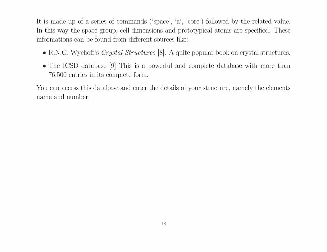
path00.dat This file contains a more exhaustive description of the paths permitting theiridentification. Here is a typical output:

Title Solid solubility of oxgen in columbium.Authors Seybolt, A.U.Reference Journal of Metals (1954) 6, 774-776Rmax 5.8000, keep limit 0.000, heap limit 0.000Plane wave chi amplitude filter 2.50%-----------------------------------------------------------------------

1 2 8.000 index, nleg, degeneracy, r= 2.8676x y z ipot label rleg beta eta

-1.655600 -1.655600 1.655600 1 ’Nb ’ 2.8676 180.0000 0.00000.000000 0.000000 0.000000 0 ’Nb ’ 2.8676 180.0000 0.00002 2 6.000 index, nleg, degeneracy, r= 3.3112x y z ipot label rleg beta eta

0.000000 -3.311200 0.000000 1 ’Nb ’ 3.3112 180.0000 0.00000.000000 0.000000 0.000000 0 ’Nb ’ 3.3112 180.0000 0.00003 3 24.000 index, nleg, degeneracy, r= 4.5232x y z ipot label rleg beta eta

1.655600 -1.655600 -1.655600 1 ’Nb ’ 2.8676 125.2644 0.0000-1.655600 -1.655600 -1.655600 1 ’Nb ’ 3.3112 125.2644 0.00000.000000 0.000000 0.000000 0 ’Nb ’ 2.8676 109.4712 0.0000

For each path it is indicated the number, scattering order and degeneracy.

It is possible to modify the atomic positions to generate (with a successive run of

genfmt) paths with new configurations using the previously calculated potentials. This

can be useful when the sample is found to have different arrangements respect to the

model crystal.

36

The successive numbers are added to better describe the path but are not considered

by genfmt. rleg is the leg length, beta indicates the photoelectron scattering angle.

Namely for path 3 in the previous example if we start from atom with potential ‘0‘

(the absorber at 0.0, 0.0, 0.0) going to the first scatterer the photoelectron travels for

2.867 A then scatters on the neighbor at (-1.655 -1.655 -1.655) with an angle of 125.2

deg, travels again for 3.311 A scatters of 125.2 deg on the neighbor at ( 1.655 -1.655

-1.655) and travels for 2.867 A before coming back to the absorber. The picture below

describes path 3 with bond lengths and angles evidenced.

��������

0

125.2 deg

r=3.311

r=2.867r=

2.867

37

7 ARTEMIS

7.1 Metallic Nb, Ist shell

For data fitting we have the the ARTEMIS code, and the picture below presents the input

page:

ARTEMIS needs the following inputs:

38

• an experimental χ(k) spectrum, extracted (namely) with ATHENA.

• the feffxxxx.dat theoretical paths generated by feff

Successively, the details for FT transformation and fit have to be added like:

• krange The range in k space for FT

• kweight n in the kn weight for exp. data

• dk The ’width’ of the window

• kwindo The window type (see manual)

• R-range The fit range in R space (if used)

• Fitting space Can be k, R or q.

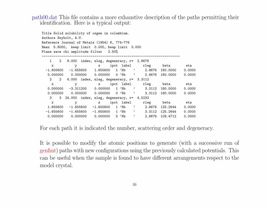
The theoretical paths to be used for the fit can be added under the menu FEFF → Add

a feff path and a window pops up with the details of the path:

39

For each path (only one in this case) a name for each variable has to be chosen to be

used in the following section. In this case we considered the number of neighbors 12 so

we decide to fir the S20 parameter, the edge shift ∆E0, the deviation from the theoretical

bond length ∆R and the Debye-Waller factor σ2.

40

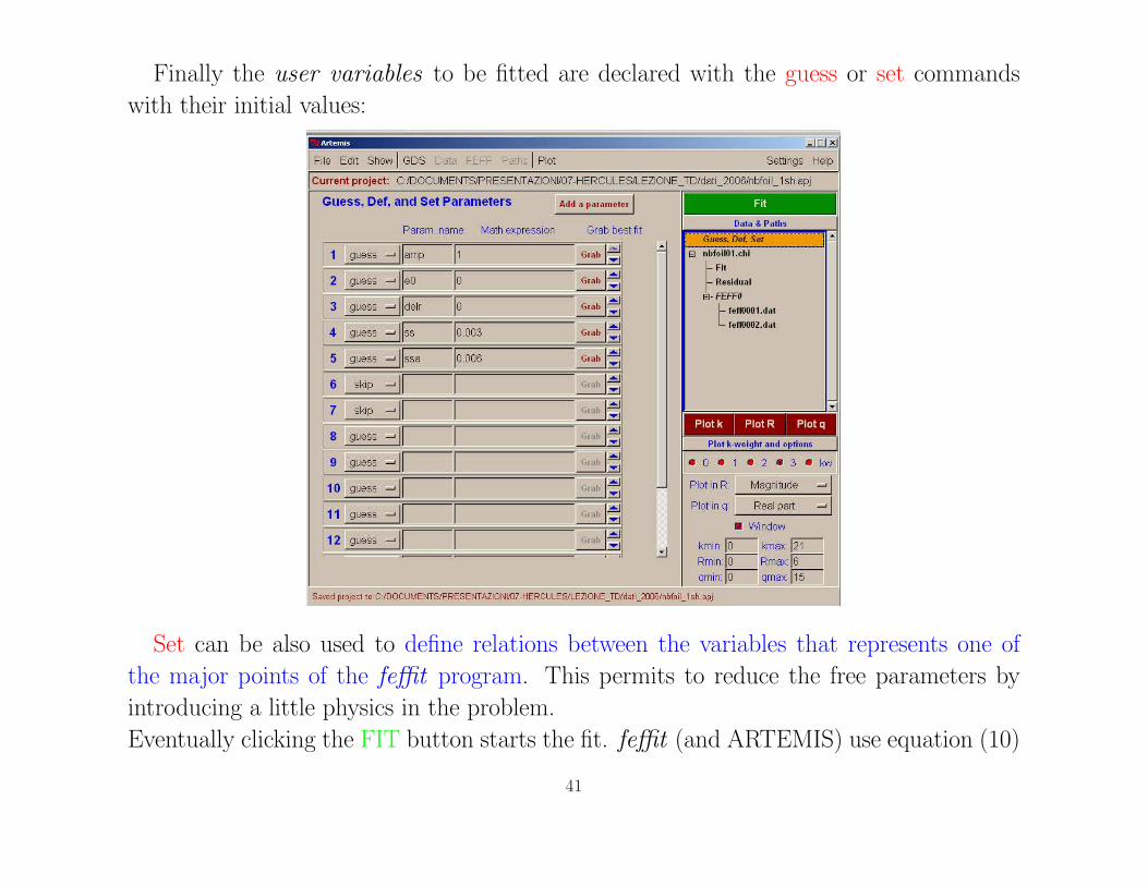
Finally the user variables to be fitted are declared with the guess or set commands

with their initial values:

Set can be also used to define relations between the variables that represents one of

the major points of the feffit program. This permits to reduce the free parameters by

introducing a little physics in the problem.

Eventually clicking the FIT button starts the fit. feffit (and ARTEMIS) use equation (10)

41

to fit data in a given R range. In this way only paths with a length less than R have to be

considered in the fit permitting the analysis on a limited frequency region of the spectrum.

The results of the fits are shown below:

The R space fit. The q space fit.

42

The results of the fits are written in the file *.log

Project title : Fitting nbfoil01.chiPrepared by :Contact :Started : 11:26:10 on 14 March, 2007This fit at : 15:26:20 on 14 March, 2007Environment : Artemis 0.6.009 using Windows XP, perl 5.006001, Tk 800.023, and Ifeffit 1.2.5

============================================================

Independent points = 15.647460938Number of variables = 5.000000000Chi-square = 10.691857339Reduced Chi-square = 1.004169670R-factor = 0.002031462Measurement uncertainty (k) = 0.000845000Measurement uncertainty (R) = 0.896066954Number of data sets = 1.000000000

Guess parameters +/- uncertainties:amp = 1.0728064 +/- 0.0333733e0 = 8.4086131 +/- 0.3872647delr = -0.0037570 +/- 0.0003963ss = 0.0036359 +/- 0.0001071ssa = 0.0038875 +/- 0.0001386

Correlations between variables:amp and ss --> 0.8790e0 and delr --> 0.8566

amp and ssa --> 0.6515

43

ss and ssa --> 0.5826All other correlations are below 0.25

===== Data set nbfoil01.chi ========================================

file: C:/DOCUMENTS/PRESENTAZIONI/07-HERCULES/LEZIONE_TD/dati_2006/nbfoil01.chititle lines:

k-range = 2.881 - 19.277dk = 2.000k-window = hanningk-weight = 3R-range = 1.851 - 3.390dR = 0.500R-window = hanningfitting space = Rbackground function = nonephase correction = none

These are not yet computed quite right in all situations...Chi-square for this data set = 506.79829R-factor for this data set = 0.00203

===== Paths used to fit nbfoil01.chi

FEFF0: feff0001.datfeff = C:\DOCUMENTS\PRESENTAZIONI\07-HERCULES\LEZIONE_TD\TEO\nb_met\feff0001.datid = reff = 2.8676, degen = 8.0, path: Nb->Nb->Nbr = 2.856826

44

reff = 2.867600degen = 8.000000n*s02 = 1.072806e0 = 8.408613dr = -0.010774reff+dr = 2.856826ss2 = 0.003636

FEFF0: feff0002.datfeff = C:\DOCUMENTS\PRESENTAZIONI\07-HERCULES\LEZIONE_TD\TEO\nb_met\feff0002.datid = reff = 3.3112, degen = 6.0, path: Nb->Nb->Nbr = 3.298760reff = 3.311200degen = 6.000000n*s02 = 1.072806e0 = 8.408613dr = -0.012440reff+dr = 3.298760ss2 = 0.003887

The fields in the file are generously commented so you can easily find all the infos you

need.

45

As a general rule in the first part the results on the ’fitted’ variables are resumed together

with the statistical analysis of the fit ( χ2 analisys, error analysis, correlations, ...).

Then the fit conditions ( weight, boundaries, ...) are shown.

Finally the results on the path variables are resumed. Note a few tricks:

• Take care to the relations you established between path and user variables.

• For the bond length R the actual fitted variable is delR. To know the R value you

have to see the value of {reff + delR}• feffit considers by default the path with its geometrical degeneracy. So in this case we

got 12 neighbours (degen) without explicitly telling the program as it went from the

calculation. If the number of neighbors is your unknown you have to run the program

with the N card = 1 and attribute to each path an amplitude S20× N where S2

0 is

found from a reference compound and N is the number of neighbors to be fitted.

46

7.2 Error analysis

A few considerations now on the error analysis made by feffit. The fitting routine works

through the minimization of a χ2-like function. For the correct statement of such a function

(in order to perform a statistical analysis on it) it is mandatory to correctly determine the

noise Epsilon on the data. When working in Fourier Transformed space it is hard to

establish a relation between the noise you can estimate on the spectrum (by the square

root of counts or by empirical techniques) and the error that propagates through the fourier

filter. An accurate error analysis is necessary to:

• decide whether what we have found is a good fit or not

• attribute error bars to the best-fitting quantities

feffit has an automatic routine that determines the ’noise’ on the data from the residual

extracted from the Fourier Transformed data between R = 15− 25 A. In this way values

of the χ2ν (χ-square function divided by the number of free parameters ν) well above 1

are obtained even for the best looking fits, preventing a correct statistical analysis. Feffit

circumvents this problem by calculating the parameters uncertainties by multiplying the

square root of the diagonal elements of the correlation matrix by√

χ2ν. This is equivalent

to rescale Epsilon to obtain a χ2ν = 1 that is to assume a priori the goodness of the fit

and attributing to statistical noise the misfit.

47

7.3 Multiple Scattering analysis

In the Fourier Transform of the metallic Nb foil several coordination shells are well visible

above the first.

Also from the feff calculation (file list.dat) several higher order paths (3 and 4 legged)

result to have a considerable amplitude.

A fit of the higher coordination shells can give a deeper insight in the material struc-

ture. Moreover for such task the inclusion of Multiple Scattering (MS) paths is mandatory.

feff has already indicated the stronger paths to be considered. By constructing our model

we only have to avoid parameter proliferation due to the increased number of paths.

With feffit path parameters can easily linked so minimizing the number of free param-

eters.

48

Below we show the input page for a 5 shell fit of metallic Nb:

49

Here the path list includes :

• Single scattering paths from the first to the fourth shell (paths 1, 2, 5, 7, 9)

1st Shell (Path 1) 2nd shell (Path 2)

3rd shell (Path 5) 4th shell (Path 7)

50

• Multiple scattering paths (paths 4, 6, 11, 12, 14)

Central - 1st - 2ndNeigh (Path 4) Central - 1st - 3rdNeigh (Path 6)

5th shell + Collinear (Path 9, 11, 12, 14)

51

The grouping of the parameters can be done as follows:

• a common value of e0 and s02 can be used for all.

• an overall scaling of the path lengths can be done by using the feffit function reff.

This can be useful when treating global expansion due to doping, temperature, ...It

can coupled to the delr variable of all paths with the command:

reff * delR

in this way for each path the length R is calculated as a fraction delR of the theoretical

length reff. delR is the only fitting parameter for the bond lengths.

• Debye-Waller factors calculated with a correlated Debye model [17]. In principle they

can be parametrized by knowing physical quantities of the system under analysis like

the interatomic force constants [16] or the Debye (or Einstein) temperatures [17], [10].

In practice this works only on a few cases.

Following these prescriptions we end up to fit the spectrum of metallic Nb up to the fifth

shell with 10 paths and only 5 free (e0, s02, delR, temp, temp1) parameters. The results

are shown below:

52

The R space fit. The q space fit.

53

The results are shown in the feffit.log file:

Project title : Fitting nbfoil01.chiPrepared by :Contact :Started : 11:26:10 on 14 March, 2007This fit at : 15:12:03 on 15 March, 2007Environment : Artemis 0.6.009 using Windows XP, perl 5.006001, Tk 800.023, and Ifeffit 1.2.5

============================================================

Independent points = 38.639648438Number of variables = 5.000000000Chi-square = 34.253119116Reduced Chi-square = 1.018236537R-factor = 0.013800488Measurement uncertainty (k) = 0.001310000Measurement uncertainty (R) = 1.389168887Number of data sets = 1.000000000

Guess parameters +/- uncertainties:amp = 1.0124631 +/- 0.0461444e0 = 7.4440333 +/- 0.4826721delr = -0.0043774 +/- 0.0004928temp = 135.0622305 +/- 7.7743092temp1 = 108.1388297 +/- 7.6940802

Correlations between variables:amp and temp1 --> 0.8825e0 and delr --> 0.8431

amp and temp --> 0.5635temp and temp1 --> 0.4974

54

All other correlations are below 0.25

===== Data set nbfoil01.chi ========================================

file: C:/DOCUMENTS/PRESENTAZIONI/07-HERCULES/LEZIONE_TD/dati_2006/nbfoil01.chititle lines:

k-range = 2.881 - 19.277dk = 2.000k-window = hanningk-weight = 3R-range = 1.851 - 5.605dR = 0.500R-window = hanningfitting space = Rbackground function = nonephase correction = none

It must be noted that the the noise level again was redefined to have a χ2ν = 1.

55

7.4 A tetrahedral compound: crystalline Ge

This is left as an exercise for the students . Here I will only suggest the atoms.inp file:

\title GEspace DIAMONDa= 5.65735rmax = 6 core= Ge

out = feff.inp

atom! Type x y z tag

Ge 0.125 0.125 0.125 Ge1--------------------

Then proceed as follows:

• Calculate the cluster

• Calculate the theoretical paths

• Try a first shell fit

• try a multiple shell (and multiple scattering) fit up to the 3rd shell.

56

8 Conclusion

Here we have briefly introduced the UWXAFS analysis package for EXAFS data. We

warmly recommend the students to further train themselves on well known structures

(bcc, zincblende, ...) to gain a full control of the various parts of the program before

approaching a real unknown sample. Due to its introductory form this lecture is far from

being exhaustive so we invite the students to refer to the programs manuals (available

on the relative web pages). Another introductory course (to which a lot of pages of the

present lecture are inspired) can be find in [20]. For further questions, feel free to contact

me at the address: dacapito@esrf.fr.

57

References

[1] P.A.Lee, P.H.Citrin, P.Eisenberger and B.M.Kincaid, Rev. Mod. Phys. 53 (1981), 769.

[2] D.C. Koningsberger, R.Prins X-ray Absorption:Principles, Applications Techniques of EXAFS, SEXAFS and XANESJohn Wiley and Sons, New York, 1988.

[3] C.R.Natoli, M.Benfatto, J. de Phys. Colloques C8 (1986), C8-11.

[4] A. Filipponi, A di Cicco, C.R.Natoli, Phys. Rev. B52, (1995), 15122.

[5] J.J.Rehr, R.C.Albers, Rev.Mod.Phys. 72,(2000), 621.

[6] J.J.Rehr, R.C.Albers, Phys.Rev B41,(1990), 8139.

[7] http://depts.washington.edu/uwxafs/

[8] R.N.G. Wychoff Crystal Structures Wiley ed., New York.

[9] http://icsd.ill.fr/icsd/

[10] S.I.Zabinsky, J.J.Rehr, A.Ankudinov, R.C.Albers, M.J.Eller, Phys.Rev B52 (1995), 2995.

[11] A.L.Ankudinov, B.Ravel, J.J.Rehr, S.D.Conradson, Phys.Rev. B58 (1998), 7565.

[12] P.A.Lee, G.Beni, Phys.Rev. B15 (1977), 2862.

[13] M.Newville, P.Livins, Y.Yacoby, J.J.Rehr, E.A.Stern, Phys. Rev. textbfB47 (1993), 14126.

[14] M. Newville, B. Ravel, D. Haskel, J. J. Rehr, E. A. Stern, and Y. Yacoby, Physica B 208&209, p154-155 (1995).

[15] http://cars9.uchicago.edu/~newville/feffit/

[16] A. Poiarkova, J.J.Rehr Phys Rev B 59 (1999), 948.

[17] E. Sevillano, H.Meuth, J.J.Rehr Phys Rev B 20 (1979), 4908.

[18] P.Eisenberger, G.S.Brown, Solid State Commun. textbf29 (1979), 481.

58

[19] G. Dalba, P.Fornasini J.Synch. Rad. 4(1997), 243.

[20] http://leonardo.phys.washington.edu/~ravel/course/Welcome.html

59