Introduction (Johannes Hanik a)

Path Tracing in ProductionPath Tracing in Productionpart 1: modern path tracingpart 2: making movies

Introduction (Johannes Hanika)Introduction (Johannes Hanika)

1

MotivationMotivationcontinued effort to:continued effort to:

document and discuss the switch of the movie industry to path tracingeducate researchers, artists, programmers, .. about the particular requirements of makingmoviesthis year: fundamentals/basics/advanced techniques

glimpse at theoretical backgroundentry points for researchstate of the arttoolset for improving rendering systems

bring together industry experts

2

Speakers (part 1)Speakers (part 1)Johannes Hanika Weta Digital, meLuca Fascione Weta Digital, Head of Technology and ResearchMarc Droske Weta Digital, Head of Rendering ResearchJorge Schwarzhaupt Weta Digital, Researcher + Manuka wizardChristopher Kulla SPI, principal so�ware engineer + Arnold veteranDaniel Heckenberg Animal Logic, R&D Supervisor, ASWF chair

3

Course notesCourse notesWhat do you need to know to write better path tracers?please see our course notes for a lot more detail!

https://jo.dreggn.org/path-tracing-in-production/2019/

4


Path tracing in ProductionPath tracing in Productionpart 1 and part 2part 2 follows in the a�ernoon

here, 403AB, 2pm-5:15pmmore about material acquisition, modelling, no Lions, and GPUs

5

Part 1: Modern path tracingPart 1: Modern path tracinghow to increase visual quality? (in order of direct relevance for movies)how to increase visual quality? (in order of direct relevance for movies)

Physics! (follows now)Mathematics! (Luca)Designing an architecture for Monte Carlo! (Marc)Special sauce sampling! (Jorge)Smoke and explosions! (Chris)Mangling crazy complex input! (Daniel)

6

Physics!Physics!

7

Recommended literatureRecommended literatureJan Novák, Iliyan Georgiev, Johannes Hanika, and Wojciech Jarosz,Monte Carlo methods for volumetric light transport simulationComputer Graphics Forum (Eurographics State of the Art Reports), 2018.Subrahmanyan Chandrasekhar,Radiative transfer,Dover Publications, 1960James Arvo,Transfer Equations in Global IlluminationSIGGRAPH Course Notes, 1993

8

PhotonsPhotonsparticle/wave dualism

we'll go with particles (for the most part), with a position and directiona photon corresponds to an atomic portion of energy (measured in Joule )

where is Planck's constant,

is the speed of light in the material with index of refraction ,and is the speed of light in vacuum,

and is the wavelength (o�en given in instead to distinguish from worldspace lengths).

we'll need a few ways to measure the energy of light

E [J]

E = [J]h ⋅ cmλ

h ≈ 6.62607004 × [ kg/s = Js]10−34 m2

= c/cm ηm ηmc = 299, 792, 458 [m/s]

λ [m] [nm]

9

Phase spacePhase spacea photon lives in 5D phase space: 3D position and 2D direction

positions are in meters

directions in steradian dimensionless, derived SI unit of solid angle

x ω

[m]

[sr]

10

Solid angleSolid anglea direction is defined on the unit sphere, areas on this sphere are called solid angle

A

Ω

r

dφdθ

as differential: or in polar form, since

we will refer to directions as and

= A/ [sr]ΩA r2

dω sin θ dθ dϕ dω = sin θ dθ dϕ = 4π∫Ω ∫ 2π0 ∫ π

0

ω Ω = 4π

11

RadianceRadiancegoal: want to measure light along a ray suitable for ray tracing

because we can only really evaluate visibility on a straight line between two pointsspoiler:

but first: let's count some photons!

L(x,ω) [ ]W

srm2

12

Radiant energyRadiant energycount number of photons inside a certain volume, multiply by their energy #P E

Q = #P ⋅ [J = ]h ⋅ cmλ

kg ⋅ m2

s2

13

Radiant power or fluxRadiant power or fluxcount photons inside certain volume per time (measured in watts):

Φ = [ = W]dQ

dt

J

s

14

Ideally: measure lightIdeally: measure lightcount photons per time in a volume in the 5D phase space over 3D positions and 2Ddirections

is a symbol "counting" photons per time going through a certain point anddirection in phase spacenote that is a 3D volume point here measured in cubic meters

V(x,ω)

Φ = P(x,ω) dxdω [W ]∫Ω

∫V

P(x,ω)

x

15

Measure radianceMeasure radiancepower per area per solid angle (measured in watts per square meter per steradian)

the central unit for us in renderingthis is what a ray of light transportsdifferentially small measurement apparatus: area with funnel

L(x,ω) = [ ]dΦ

dxdω

W

srm2

16

Measure radiance?Measure radiance?dynamic system, light is in flowdescribe changes of radiance in phase space and solve for steady-state equilibrium!

17

Losses and gainsLosses and gainsthree effects change the observed amount of light:

collision: light interacts with matteremission: light is emitted from matterstreaming: light enters or leaves a volume

collision may incur scattering: change of direction

18

The radiative transfer equation (RTE)The radiative transfer equation (RTE)summing all termssumming all terms

all terms need to sum to zero (energy conservation)

if the equations hold for integration over any part of phase space, they have to hold forevery individual point, tooleave away integration over phase space

0 = ∫Ω

∫V

− +L(x,ω)∂

∂ω

streaming

(x) (x,ω)μe Le

emission

− (x)L(x,ω)μt

extinction

+ dx dω(x) ( ⋅ ω)L(x, )dμs ∫Ω

fs ωi ωi ωi

in-scattering

Ω × V

19


all terms need to sum to zero (energy conservation), lose phase space integral

we are interested in changes in radiance the directional derivative (LHS) is change of radiance in direction

L(x,ω)∂

∂ω

streaming

= (x) (x,ω)μe Le

emission

− (x)L(x,ω)μt

extinction

+ (x) ( ⋅ ω)L(x, )dμs ∫Ω

fs ωi ωi ωi

in-scattering

L(x,ω)

L(x,ω)∂∂ω ω

20


integro differential equation along one ray governs scattering in participating media (volumes)we need to bring it to pure integral form for graphics applications!

L(x,ω)∂

∂ω= (x) (x,ω) − (x)L(x,ω)μe Le μt

+ (x) ( ⋅ ω)L(x, )dμs ∫Ω

fs ωi ωi ωi

(x,ω)

21

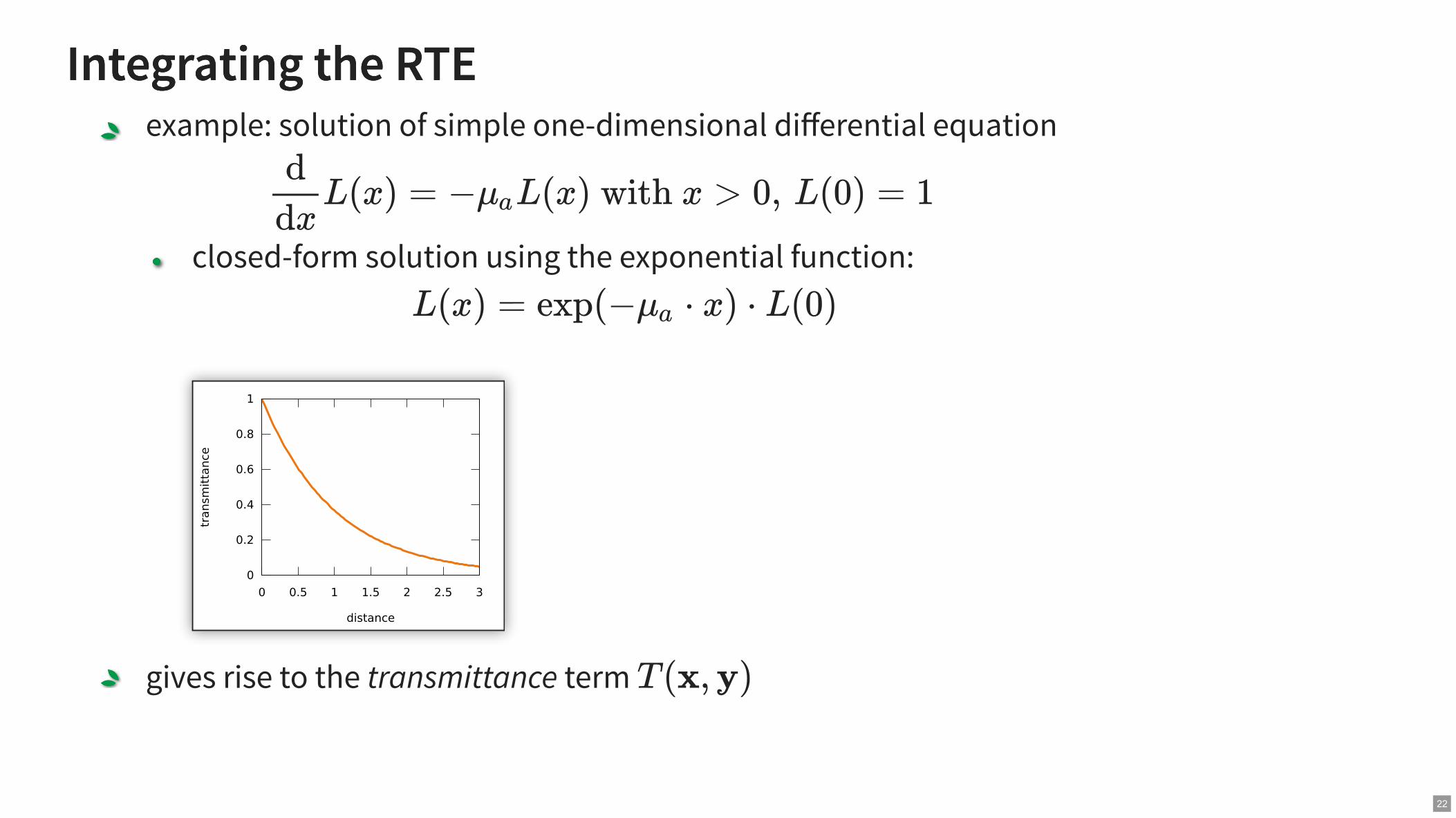
Integrating the RTEIntegrating the RTEexample: solution of simple one-dimensional differential equation

closed-form solution using the exponential function:

0

0.2

0.4

0.6

0.8

1

0 0.5 1 1.5 2 2.5 3

transmittance

distance

gives rise to the transmittance term

L(x) = − L(x) with x > 0, L(0) = 1d

dxμa

L(x) = exp(− ⋅ x) ⋅ L(0)μa

T(x, y)

22

The RTE in integral formThe RTE in integral formIntegrating the RTE: intuitionIntegrating the RTE: intuition

contribution from surface emission (exactly one point )

yx

y

L(x,ω) += T(x, y) ⋅ (y,ω)Le

23


contribution from surface scattering (exactly one point )

yx

y

L(x,ω) += T(x, y) ⋅ ( , y,ω)L(y, )d∫Ω

fr ωi ωi ω⊥i

24


contribution from volume emission (need to collect all )

zx

z

L(x,ω) += T(x, z) ⋅ (z) (z,ω)μe Le

25


contribution from volume scattering (need to collect all )

zx

z

L(x,ω) += T(x, z) ⋅ (z) (ω ⋅ )L(z, )dμs ∫Ω

fs ωi ωi ωi

26

The RTE in integral formThe RTE in integral form

z y

dt

x

L(x,ω) = T(x, y)( (y,ω) + ( , y,ω)L(y, )d )Le ∫Ω

fr ωi ωi ω⊥i

contribution from the point y on surface

+ T(x, z) dt∫d

0( (z) (z,ω) + (z) (ω ⋅ )L(z, )d )μe Le μs ∫

Ω

fs ωi ωi ωi

contribution from any point z at distance t in volume

27

Recursive rendering equationRecursive rendering equationlight is emission + transported light (either from surface or volume)

Neumann series ( is a linear operator):

turns recursion into sum over all path lengths!

L = + TLLe

T

L = (1 − T =)−1Le ∑i=0

∞

TiLe

28

Tracing paths the recursive wayTracing paths the recursive waymeans tracing rays, usually through every pixel

29

Tracing paths the recursive wayTracing paths the recursive waymeans tracing rays, usually through every pixel

recursive rendering equation: light is emission + transported lightL = + TLLe

30

The rendering equation in path integral formThe rendering equation in path integral formexpand using the Neumann series to arrive at path space

selects paths per pixel via pixel filter supportpath is list of vertices

is the measurement contribution function in product vertex area measure

= (X) ⋅ f(X)dXIp ∫P

hp

(X)hp p

X = ( , , . . . ) ∈ Px1 x2 xk x

f(X) dX

31

The measurement contribution functionThe measurement contribution functionmeasure differential power of path with length ( vertices here)X k = 5

f(X) = ( )WLeGk−1 ∏i=1

k−2

fr,iGi

32

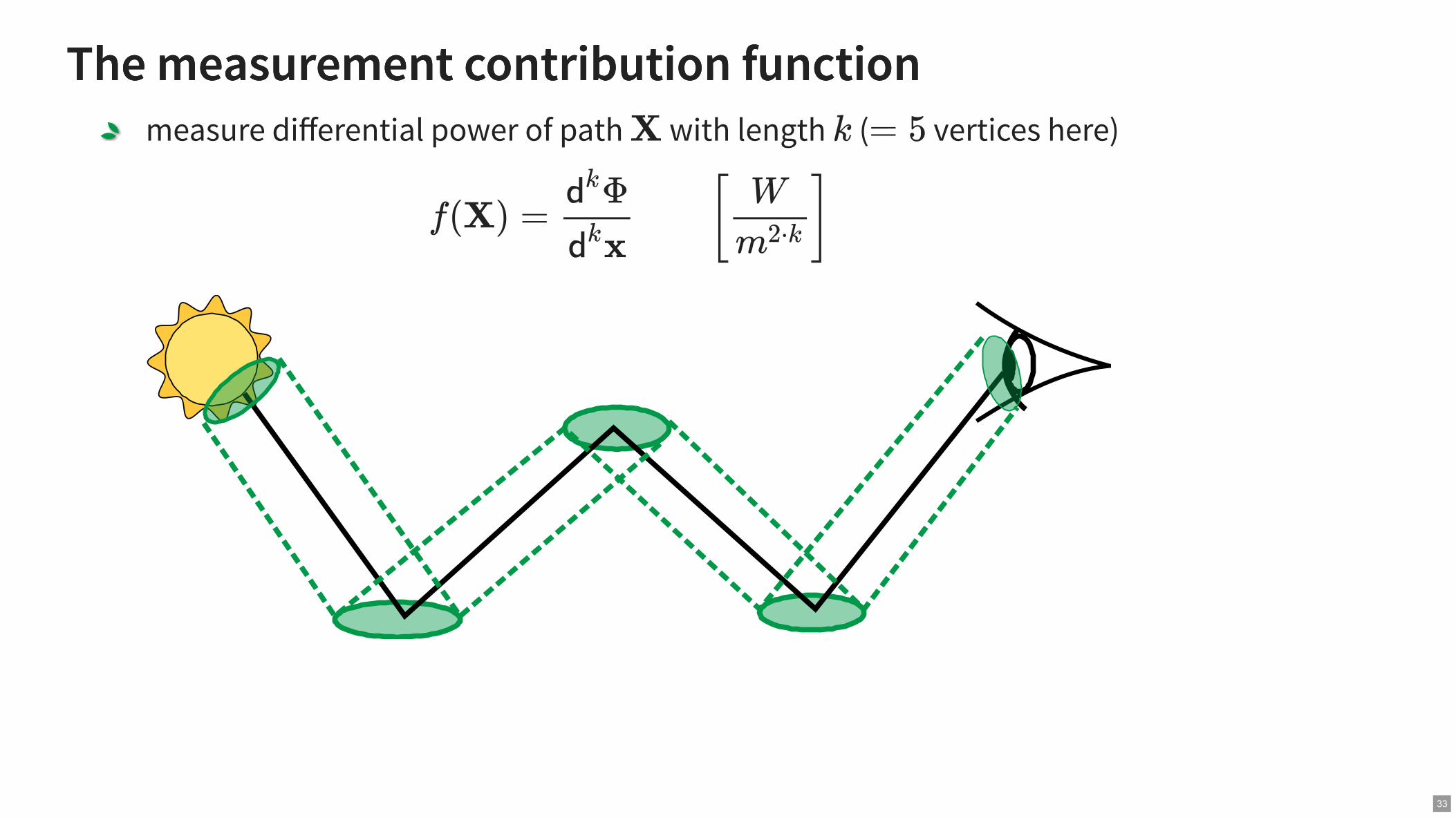
The measurement contribution functionThe measurement contribution functionmeasure differential power of path with length ( vertices here)X k = 5

f(X) = [ ]Φd

k

xdk

W

m2⋅k

33

Monte Carlo integrationMonte Carlo integrationapproximate the integral by a Monte Carlo estimator

the expected value of the estimator is precisely the integral (the estimator is unbiased)error manifests itself as noise (variance of the estimator)

how much noise for which path construction strategy determined by their PDF

≈Ip1

N∑i=1

N ( ) ⋅ f( )hp Xi Xi

p( )Xi

p(X)

34

Path tracingPath tracingstart constructing a path at the sensorsample outgoing direction locally by Bsdf

35

Path tracingPath tracingstart constructing a path at the sensorproblem intersecting light source by chance

36

Path tracing/next event estimationPath tracing/next event estimationstart constructing a path at the sensordirect connection(s) to light source in area measure

37

Path tracing/next event estimationPath tracing/next event estimationproblem connecting glossy/specular materialsBsdf evaluates to zero (or close to for low roughness > 0)

38

Light tracingLight tracingreverse the tracing direction, start at the light sourcesgood for caustics

39

Light tracingLight tracing..but doesn't work for specular, eitherSDS doesn't work even for combination of all the above techniques (called BDPT)

40

Vertex connection and merging (VCM/UPS)Vertex connection and merging (VCM/UPS)uses photon maps to cover SDS pathsexpensive: big storage, long kd-tree build times, many combinations to evaluate

41

Metropolis light transport (MLT)Metropolis light transport (MLT)mutates initial sample, uses current path as Markov chain stateo�en leads to temporal inconsistency/blotches

42

Production images omitted for publicationProduction images omitted for publication:(

43

Program part 1:Program part 1:09:00 — Opening statement and introduction to path tracing (almost over now!)(30 min, Johannes Hanika)09:30 — A short History of Monte Carlo(30 min, Luca Fascione)10:00 — Implementing path sampling techniques(30 min, Marc Droske)10:30 — Break (15 min)

44

Program part 1, cntd:Program part 1, cntd:10:45 — Finding good paths(30 min, Jorge Schwarzhaupt)11:15 — Volumes(30 min, Christopher Kulla)11:45 — The Ins of Production Rendering at Animal Logic(30 min, Daniel Heckenberg)

45

Path tracing in production, part 2Path tracing in production, part 2will continue in the a�ernoon sessionwill continue in the a�ernoon session

here, 403AB, 2pm-5:15pm

46

Let's get started!Let's get started!

47

Thank you for listeningThank you for listeningquestions?questions?

please find our course notes here:https://jo.dreggn.org/path-tracing-in-production/2019/

48


Introduction (Johannes Hanik a)

Documents

Transcript of Introduction (Johannes Hanik a)