International Journal of Remote Sensing Integration of ...

PLEASE SCROLL DOWN FOR ARTICLE

This article was downloaded by: [Fang, Hongliang]On: 5 March 2011Access details: Access Details: [subscription number 934407021]Publisher Taylor & FrancisInforma Ltd Registered in England and Wales Registered Number: 1072954 Registered office: Mortimer House, 37-41 Mortimer Street, London W1T 3JH, UK

International Journal of Remote SensingPublication details, including instructions for authors and subscription information:http://www.informaworld.com/smpp/title~content=t713722504

Integration of MODIS LAI and vegetation index products with the CSM-CERES-Maize model for corn yield estimationHongliang Fangab; Shunlin Lianga; Gerrit Hoogenboomc

a Department of Geography, University of Maryland, College Park, MD, USA b NASA Goddard EarthSciences Data and Information Services Center (GES DISC) employed by Wyle Information Systems,McLean, Virginia, USA c Department of Biological and Agricultural Engineering, University ofGeorgia, Griffin, GA, USA

Online publication date: 04 March 2011

To cite this Article Fang, Hongliang , Liang, Shunlin and Hoogenboom, Gerrit(2011) 'Integration of MODIS LAI andvegetation index products with the CSM-CERES-Maize model for corn yield estimation', International Journal of RemoteSensing, 32: 4, 1039 — 1065To link to this Article: DOI: 10.1080/01431160903505310URL: http://dx.doi.org/10.1080/01431160903505310

Full terms and conditions of use: http://www.informaworld.com/terms-and-conditions-of-access.pdf

This article may be used for research, teaching and private study purposes. Any substantial orsystematic reproduction, re-distribution, re-selling, loan or sub-licensing, systematic supply ordistribution in any form to anyone is expressly forbidden.

The publisher does not give any warranty express or implied or make any representation that the contentswill be complete or accurate or up to date. The accuracy of any instructions, formulae and drug dosesshould be independently verified with primary sources. The publisher shall not be liable for any loss,actions, claims, proceedings, demand or costs or damages whatsoever or howsoever caused arising directlyor indirectly in connection with or arising out of the use of this material.

http://www.informaworld.com/smpp/title~content=t713722504

http://dx.doi.org/10.1080/01431160903505310

http://www.informaworld.com/terms-and-conditions-of-access.pdf

Integration of MODIS LAI and vegetation index products with theCSM–CERES–Maize model for corn yield estimation

HONGLIANG FANG†‡*, SHUNLIN LIANG† and GERRIT HOOGENBOOM§

†Department of Geography, University of Maryland, College Park, MD 20742, USA

‡NASA Goddard Earth Sciences Data and Information Services Center (GES DISC)

employed by Wyle Information Systems, McLean, Virginia, USA

§Department of Biological and Agricultural Engineering, University of Georgia, Griffin,

GA 20223, USA

(Received 14 May 2009; in final form 20 November 2009)

Advanced information on crop yield is important for crop management and food

policy making. A data assimilation approach was developed to integrate remotely

sensed data with a crop growth model for crop yield estimation. The objective was to

model the crop yield when the input data for the crop growth model are inadequate,

and to make the yield forecast in the middle of the growing season. The Cropping

System Model (CSM)–Crop Environment Resource Synthesis (CERES)–Maize and

the Markov Chain canopy Reflectance Model (MCRM) were coupled in the data

assimilation process. The Moderate Resolution Imaging Spectroradiometer

(MODIS) Leaf Area Index (LAI) and vegetation index products were assimilated

into the coupled model to estimate corn yield in Indiana, USA. Five different

assimilation schemes were tested to study the effect of using different control vari-

ables: independent usage of LAI, normalized difference vegetation index (NDVI) and

enhanced vegetation index (EVI), and synergic usage of LAI and EVI or

NDVI. Parameters of the CSM–CERES–Maize model were initiated with the remo-

tely sensed data to estimate corn yield for each county of Indiana. Our results showed

that the estimated corn yield agreed very well with the US Department of Agriculture

(USDA) National Agricultural Statistics Service (NASS) data. Among different

scenarios, the best results were obtained when both MODIS vegetation index and

LAI products were assimilated and the relative deviations from the NASS data were

less than 3.5%. Including only LAI in the model performed moderately well with a

relative difference of 8.6%. The results from using only EVI or NDVI were unaccep-

table, as the deviations were as high as 21% and -13% for the EVI and NDVI

schemes, respectively. Our study showed that corn yield at harvest could be success-

fully predicted using only a partial year of remotely sensed data.

1. Introduction

Reliable and timely prediction of crop yield is important for agricultural land man-

agement and policy making. Many studies have demonstrated the utilization of

satellite data in crop yield estimation. Country-level crop yield estimation using

*Corresponding author. Now at: The State Key Laboratory of Resources and

Environmental Information System (LREIS), Institute of Geographic Sciences and

National Resources Research, Chinese Academy of Sciences (CAS), Beijing 100101,

China. Email: [email protected]

International Journal of Remote SensingISSN 0143-1161 print/ISSN 1366-5901 online # 2011 Taylor & Francis

http://www.tandf.co.uk/journalsDOI: 10.1080/01431160903505310

International Journal of Remote Sensing

Vol. 32, No. 4, 20 February 2011, 1039–1065

Downloaded By: [Fang, Hongliang] At: 06:03 5 March 2011

remote sensing data has been carried out operationally for more than two decades

(MacDonald and Hall 1980). Vegetation indices calculated from Thematic Mapper

(TM) data have improved the accuracy of ground wheat yield surveys through

stratification of primary sampling units (Singh et al. 1992). Promising results have

been obtained through the statistical relationship between satellite reflectance valuesor vegetation indices and crop yield (Thenkabail et al. 1992, Jiang et al. 2003, Kogan

et al. 2005, Weissteiner and Kuhbauch 2005). However, these methods are mainly

empirical and they may work only for specific crop cultivars, a particular crop growth

stage or environmental conditions at specific times.

Integration of remote sensing and crop growth simulation models has become

recognized increasingly as a potential tool for crop growth monitoring and yield

estimation (Abou-Ismail et al. 2004, Mo et al. 2005, Jongschaap 2006, Dente et al.

2008, Liang and Qin 2008). Several assimilation schemes with different degrees ofcomplexity and integration have been developed during the last two decades (Maas

1988a, Delecolle et al. 1992, Moulin et al. 1998, Baret et al. 2000, Plummer 2000). Maas

(1988a, b) initially reviewed different methods for combining a crop simulation model

with radiometric observations (ground measurements or satellite data). Delecolle et al.

(1992) generalized them into four methods: (1) directly using remotely sensed variables

in the model; (2) updating state variables in the model; (3) re-initialization of the model;

and (4) re-parametrization of the model. Re-parametrization is similar to re-

initialization except that the model parameters are adjusted (Plummer 2000). Puttingsatellite products into crop growth models in the re-parametrization procedure corre-

sponds to the highest degree of integration (Baret et al. 2000).

The essence of the data assimilation approach is to improve the initial parametriza-

tion of the crop growth model and augment simulation with the use of remotely

sensed observations. Different researchers have used Leaf Area Index (LAI), spectral

reflectance or vegetation indices as a control variable to adjust or to determine the

optimal set of input parameters (e.g. Bach et al. 2001, 2003, Doraiswamy et al. 2003,

Fang et al. 2008). Maas (1988a) and Dente et al. (2008) used remotely sensed LAI inthe adjustment of model initial conditions to minimize the difference between model-

predicted and remotely estimated LAI. Moulin et al. (1998) coupled a crop produc-

tion model and a radiative transfer model, compared a simulated reflectance profile

with a satellite-measured reflectance, and successfully re-tuned crop model para-

meters and initial conditions. Weiss et al. (2001) successfully assimilated the radiative

transfer model SAIL and a crop growth model (STICS); simulated and measured

reflectances agreed very well. Combining the process model (PROMET-V) with the

canopy radiative transfer model Scattering by Arbitrarily Inclined Leaves (SAIL),Bach et al. (2001) obtained very good results for LAI, dry biomass and canopy height.

De Wit (1999) integrated the World Food Studies (WOFOST) model (Boogaard et al.

1998) and satellite vegetation index data to retrieve wheat and sunflower conditions.

Guerif and Duke (2000) also reported the usefulness of vegetation indices, especially

for estimating the planting date and emergence parameters.

However, little work has been done to compare the performances by assimilating

different satellite products, such as LAI and vegetation index. Doraiswamy et al.

(2004) indicated that integrating remotely sensed LAI with a crop growth model haslimitations and the data assimilation procedure needs further improvement. One

major issue is related to the difficulty of obtaining an accurate LAI estimation from

remotely sensed data. This limits the application of the data assimilation method at

regional scales. Guerif and Duke (2000) compared the effect of spectral reflectance

1040 H. Fang et al.


and vegetation index and discovered that using a vegetation index was a better choice

than spectral reflectance because the assimilation was very sensitive to variables such

as soil reflectance and leaf optical properties in the canopy radiative transfer models.

In a previous study, Fang et al. (2008) developed an integrated crop simulation

model, successfully estimating corn yield by integrating a crop growth model with theModerate Resolution Imaging Spectroradiometer (MODIS) LAI products. This

study extends that earlier work by assimilating both LAI and vegetation indices

into the coupled crop growth and radiative transfer model in order to improve the

estimation of crop yield on a county level. The effect of assimilating LAI separately

and LAI and vegetation index synergistically was also studied. The next section

presents the assimilation method, including crop model data preparation, remotely

sensed data pre-processing, and different optimization schemes. The Cropping

System Model (CSM)–Crop Environment Resource Synthesis (CERES)–Maizecrop growth model and the Markov canopy reflectance model are presented. A

sensitivity evaluation of the canopy reflectance model is introduced to determine

the set of free parameters for the model. The results are analysed in the third section.

Section four discusses the potentials and challenges of the data assimilation approach,

followed by a conclusion section at the end of the paper.

2. Data assimilation method

The general methodology of the data assimilation method is illustrated in figure 1.

Three steps were involved in this procedure.

Crop growthmodel

Canopy radiativetransfer model

Crop yield,water balance

Crop, soil,management

Remotesensing data

Vegetationindices

LAI

Weather andclimate

Yes

No

Calculation ofJi (eqs (6)–(8))

MinimizesJi?

Figure 1. General methodology of the data assimilation approach integrating remote sensingdata with crop growth and canopy reflectance models for crop yield estimation.

Corn yield estimation 1041


1. Input data, such as crop characteristics, soil condition, management

practice and weather information, were prepared in advance for the

CSM–CERES–Maize model. A list of free variables is shown in table 1. With

these input data, crop biophysical information (e.g. LAI) was generated by the

crop growth model.

2. The parameters simulated by the crop model (e.g. LAI) and other ancillary

information (e.g. soil reflectance) were used in the canopy reflectance model.Vegetation indices were calculated from the simulated reflectances.

3. The simulated vegetation indices and LAI were compared with the correspond-

ing MODIS products, and residuals between the simulated and MODIS LAI or

vegetation index were minimized by adjusting the input parameters in step 1.

With the optimized set of input parameters, the model was executed to update

the crop yield prediction.

2.1 Material and models

Our study area was the state of Indiana, USA, ranging from 37� 460 N to 41� 460 N

and 84� 470 W to 88� 60 W. The topography of Indiana is characterized by vast flatplains in the northern two-thirds of the state and rugged hills in the southern. Indiana

has a humid continental climate, with an annual precipitation of around 1000 mm.

Corn and soybean are the two dominant crops. The average size of a farm is 240 ha.

The prime planting period for corn is from late April to late May, while the typical

harvesting period is from late September to early November. The statistical corn yield

was obtained from the US Department of Agriculture (USDA) National Agricultural

Statistics Service (NASS) reports for most counties in the state.

2.1.1 Crop growth and canopy reflectance models. The CSM–CERES–Maize model

is a functional crop model that simulates growth, development and yield of corn under

different weather, soil and management conditions (Jones et al. 2003). The

CSM–CERES–Maize model used in this study was encompassed in the DecisionSupport System for Agrotechnology Transfer (Tsuji et al. 1994, Hoogenboom et al.

1999, 2004) package. The CSM–CERES–Maize model simulates phenological develop-

ment, vegetative and reproductive plant development stages, partitioning of assimilates,

growth of leaves and stems, senescence, biomass accumulation and root system

dynamics. It has been used to predict grain yield and kernel numbers (Kiniry et al.

1997, Asadi and Clemente 2001, Lizaso et al. 2001, Tojo Soler et al. 2007), the effects of

ground water and precipitation (Xie et al. 2001, O’Neal et al. 2002) and the effect of

Table 1. Free parameters and their range in the coupled crop growth andcanopy reflectance model.

Variables Range

Crop growth model (CSM–CERES–Maize)Planting date (day of year) 98–158Planting population (plants m-2) 6.0–7.5Row spacing (cm) 75–90Nitrogen amount in fertilizer (kg ha-1) 20–180Canopy reflectance model (MCRM)Soil reflectance (red band) 0.02–0.5Effective number of elementary layers in a leaf 1.0–3.0

1042 H. Fang et al.


increasing atmospheric carbon dioxide (Tubiello et al. 1999). The model has performed

very well for predicting corn yield. For example, the relative errors are as low as 6.2% and

5%, as reported by Asadi and Clemente (2001) and Kiniry et al. (1997), respectively.

The Markov Chain Reflectance Model (MCRM) (Kuusk 1998) was used to simulate

the reflectance at the top of the canopy. The Markov model simulates two-layer canopyreflectances at different solar illumination and viewing geometries (Kuusk 2001). In the

MCRM model the canopy is assumed to be horizontally uniform above a horizontal

ground surface. Leaf optical properties are simulated with the PROSPECT model

(Jacquemoud and Baret 1990). The model was validated by the developers (Kuusk

et al. 1997) and it performs very well in terms of accuracy and running time, and has

been proved useful for crop canopy (Kuusk 1998, Jacquemoud et al. 2000, Fang and

Liang 2003). Reflectances simulated by the Markov model for the top of canopy were

used to compute the vegetation indices. The normalized difference vegetation index(NDVI) was calculated using the following equation:

NDVI ¼ rNIR � rR

rNIR þ rR

: (1)

where rR and rNIR are surface reflectances of the red and near-infrared bands,

respectively. The enhanced vegetation index (EVI) was calculated as:

EVI ¼ G rNIR � rRð ÞrNIR þ C1rR � C2rB þ L

; (2)

where rB is the surface reflectance in the blue band, L is the canopy background

adjustment and C1 and C2 are the coefficients of the aerosol resistance term. The

coefficients used in the EVI calculation are L¼ 1, C1¼ 6, C2¼ 7.5 and G (gain factor)

¼ 2.5 (Huete et al. 2002).

2.1.2 Evaluation of the canopy reflectance model. The number of free parameters iscrucial in data assimilation. Sensitivity studies were conducted to identify the critical

parameters for the crop growth model (Fang et al. 2008). An evaluation of the

Markov model is indispensable to identify the optimal set of free parameters. Some

studies have found that the optimization process is more robust if the number of free

parameters is small (Kimes et al. 2000, Qin et al. 2008). Kimes et al. (2000) suggested

that for radiative transfer model inversion, the number of free parameters that

significantly impact the canopy reflectance ought to be minimal.

Among different algorithms for the radiative transfer model optimization, thegenetic algorithm (GA) was used to determine the best set of free parameters.

Genetic algorithm simulates the process of natural selection and evolutionary genetics.

A detailed introduction of genetic algorithms can be found in Davis (1991) and

Goldberg (1989). The general process is to adjust the radiative transfer model input

parameters (genes in genetic algorithms) so that a simulated reflectance by the radiative

transfer model agrees with the corresponding MODIS observation. Then some para-

meters that change less rapidly are fixed and the previous step is repeated until an

optimal set of parameters is obtained. The advantage of using genetic algorithms is thatit avoids the initial guess selection problem and provides a systematic scanning of the

whole acceptable solution such that a global optimum solution could be reached.

The input parameters of the forward Markov model are summarized in table 2. The

solar zenith angle (SZA) represents the values applicable to when the MODIS data

were acquired. The leaf water content and leaf dry matter content (protein, cellulose



and lignin) are from Jacquemoud et al. (1996). The sensitivity of the hot-spot para-

meter SL (¼ 0.15) in the inversion is very low. Seven free parameters (or genes) were

identified: LAI, Sz, leaf angle distribution (LAD), Cab, N, rs1, and rs2. Their effective

ranges are displayed in table 2.

The simulated reflectances in the red and NIR bands were compared with MODIS

reflectances. These two spectral bands were selected because they are the mostfrequently used bands in biophysical parameter retrieval (e.g. the MODIS LAI

products) and they performed equally when compared to using more than two

channels (Fang and Liang 2003, 2005). In this study, we started with testing all

seven genes with the goal of finding the most sensitive ones. An example of the

retrieved values for the seven parameters on day of year (DOY) 185 is shown in

figure 2. Their mean, standard deviation (STD) and coefficient of variance (CV)

values over the whole study area were also calculated. The Markov parameter

describing clumping (Sz) was found to be the most stable variable in the study area,with a mean of 0.81 and the lowest CV (0.11). Other parameters, such as LAI and N,

illustrate more heterogeneous conditions over the area. In this case, Sz ¼ 0.81 was

chosen to represent the general status of the study area and was fixed in the next

iterations. In a similar fashion, a representative Sz value was derived for other days

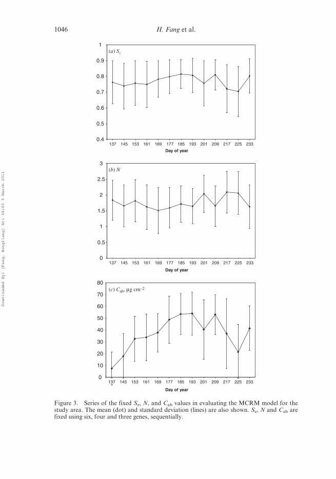
over the growing season (figure 3).

After Sz was fixed, a similar optimization procedure was applied to identify other

less variable parameters. Starting with seven free parameters, Sz, LAD, N and Cab

were fixed sequentially with the number of genes reduced from 7 to 3. It is reason-able to assume that when the number of free parameters is decreased, the retrieved

LAD, N and Cab values may differ from those in the previous iteration. The times-

series of the fixed values in figure 3 represent the general conditions of the study area

in the assimilation experiments. The Markov parameter (Sz) ranges from 0.70–0.81

Table 2. Input parameters for the MCRM radiative transfer model.

Parameters Symbol Values

External parametersSolar zenith angle (�) SZA (from MODIS data)Angstrom turbidity factor t 0.1

Canopy structure parametersLeaf area index* LAI 0–10.0Leaf linear dimension/canopy height ratio SL 0.15Markov parameter describing clumping* SZ 0.4–1.0Leaf angle distribution* LAD 0–90.0

Leaf spectral and directional propertiesChlorophyll AB concentration (mg cm-2)* Cab 0–90Leaf equivalent water thickness (cm) Cw 0.01Leaf protein content (g cm-2) Cp 0.001Leaf cellulose and lignin content (g cm-2) Cc 0.002Leaf structure parameter* N 0.5–3.5

Soil spectral and directional properties (Price 1990)First weight of the Price function* rs1 0–1.0Second weight of the Price function* rs2 -1.0–1.0Third and fourth weights of the Price function rs3, rs4 0.0

*Free parameter

1044 H. Fang et al.


over the growing season. A very stable value of LAD was observed when six genes

were tested and thus leaf angle distribution (49.1�) was set to a constant value for the

entire growing season. The retrieved leaf structure parameter (N) scatters between

1.0 and 3.0. The mean chlorophyll content (Cab) showed a general increase from 7.5

mg cm-2 on day 137 to 54.0 mg cm-2 on day 193. After the maturity onset day (see§2.3.1 for the corresponding phenological stage), the retrieved Cab became very

unstable, ranging from 0.0 mg cm-2 to 90.0 mg cm-2 for the whole study area. LAI

and soil reflectance (rs1 and rs2) are the final parameters that were not fixed in the

optimization process, indicating that they were very critical for the canopy reflec-

tance simulation.

0

1

2

3

4

5

6

7

8

9

10

(a) LAI, Mean/STD/CV: 4.09/1.68/0.41

0.0

0.1

0.2

0.3

0.4

0.5

0.6

0.7

0.8

0.9

1.0

(b) Sz, 0.81/0.09/0.11

0

10

20

30

40

50

60

70

80

90

(c) LAD, 45.1/13.32/0.30

0

10

20

30

40

50

60

70

80

90

100

(d) Cab, 45.92/17.87/0.39

0.0

0.5

1.0

1.5

2.0

2.5

3.0

3.5

4.0

(e) N, 1.04/0.55/0.53

0.0

0.1

0.2

0.3

0.4

0.5

0.6

0.7

0.8

0.9

1.0

(f) rs1, 0.43/0.14/0.33

(g) rs2, –0.016/0.040/–2.43

-0.15

-0.10

-0.05

0.00

0.05

0.10

0.15

0 200 400 600 800

Pixel

0 200 400 600 800 Pixel 0 200 400 600 800

0 200 400 600 800 0 200 400 600 800

0 200 400 600 800 0 200 400 600 800

Figure 2. The sorted values of LAI, Sz, LAD, Cab, N, rs1 and rs2 derived from the GAoptimization method for all pixels in the study area on day 185. The abscissa represents thecorn pixels in the study area. The thin lines show their corresponding standard deviation in theGA retrieval. The overall mean, standard deviation and coefficient of variation (CV) are alsocalculated.



0.4

0.5

0.6

0.7

0.8

0.9

1

137 145 153 161 169 177 185 193 201 209 217 225 233

Day of year

(a) Sz

0

0.5

1

1.5

2

2.5

3

137 145 153 161 169 177 185 193 201 209 217 225 233

(b) N

Day of year

0

10

20

30

40

50

60

70

80

137 145 153 161 169 177 185 193 201 209 217 225 233

(c) Cab, µg cm–2

Day of year

Figure 3. Series of the fixed Sz, N, and Cab values in evaluating the MCRM model for thestudy area. The mean (dot) and standard deviation (lines) are also shown. Sz, N and Cab arefixed using six, four and three genes, sequentially.

1046 H. Fang et al.


2.2 Data preparation for model integration

2.2.1 Input data for the crop growth model. Crop yield is influenced strongly by

local cultivar characteristics, soil and weather conditions, and crop management. It

may vary considerably in different fields and calendar years. The input parameters for

the crop growth model include soil types, planting dates, planting rates and local

weather data. For a local application (e.g. Guerif and Duke 2000), the initial condi-

tions and the model parameters of crop leaf and soil optical properties are usually

assumed to be known. Extending from a local to a large region requires automatic

estimation of some of these parameters on a pixel basis.Daily weather data, soil properties and crop ecology and management information

are required to run the crop simulation model. Soil texture data from the USDA State

Soil Geographic (STATSGO) database were used (http://www.ncgc.nrcs.usda.gov/

branch/ssb/products/statsgo/index.html). Daily weather data were obtained from the

North America Land Data Assimilation Systems (NLDAS) (http://ldas.gsfc.nasa.

gov) because the data are spatially continuous with a high spatial resolution (1/8�).The soil and weather data were re-projected to a 1 km resolution.

Other crop growth studies have identified various parameters that are critical forLAI simulation. Bouman (1992) and Clevers et al. (1994) suggested using the ‘light use

efficiency’ and ‘maximum leaf area’, while Maas (1988a) worked with the ‘initial

LAI’. Jongschaap (2006) experimented with the impact of field water content on

simulated LAI. An earlier sensitivity analysis was conducted to identify the most

critical parameters for crop model simulation (Fang et al. 2008). Some crop manage-

ment variables, such as the corn cultivar type, planting date, planting population and

row spacing, were found to be very critical for the execution of the CSM–CERES–

Maize model (Fang et al. 2008). Pioneer cultivars (PC0003) represent the overwhelm-ing majority of corn cultivars planted in Indiana and were used in the study. The

planting date, planting population and row spacing were free variables and were

estimated on a pixel basis (table 1). The USDA NASS reports provide the average

planting date for each crop at the state level. The statistical planting date was used to

determine their initial values for crop growth simulation (http://www. nass.usda.gov/

in/annbul/0304/04weather.html).

The nutrient supply is represented by the application of nitrogen, which was set as a

free variable. The date of nitrogen application was set to the same date as the plantingdate.

An initial parametrization was conducted by adjusting the CSM–CERES–Maize

model to the USDA NASS corn yield at the state level. A list of values for all the free

parameters was generated as a starting point for the pixel-specific calibrations in the

optimization process.

2.2.2 Input data for the canopy radiative transfer model. For canopy biophysical

and structural properties, such as the Markov parameter (Sz) and LAD, results from

the above genetic algorithm optimization were applied (§2.1.2). Reference values fromfield measurements and remote sensing retrievals for similar corn fields were adopted

for the leaf water and dry mater contents (table 2). The chlorophyll content of the leaf

(Cab) and the effective number of elementary layers inside a leaf (N) are crucial in the

Markov model to simulate the leaf optical properties (Kuusk 1998). The current

CSM–CERES–Maize model does not treat leaf chlorophyll content as an output

even though the chlorophyll content could be estimated based on a correlation with

the leaf nitrogen amount (Bullock and Anderson 1998). In this study, the leaf



chlorophyll content was fixed in order to focus on the effect of leaf structure and soil

reflectance (table 1).

The soil reflectance (represented in the Price function) is an important parameter in

the Markov model. In this study, an empirical method was developed to calculate thesoil reflectance. The soil reflectance in the red band was set as a free variable between

0.02 and 0.50 (table 2). The soil reflectances for the blue, green and NIR bands were

derived using the regression relationship (figure 4) created from the soil reflectance

libraries provided by Daughtry (2001) and Dr J. Salisbury at the Johns Hopkins

University (Jet Propulsion Laboratory 1998):

rB ¼ 0:397rR þ 0:004

rG ¼ 0:697rR � 0:002;

rNIR ¼ 1:105rR þ 0:060

(3)

where rB, rG, rR and rNIR represent surface reflectances of the blue, green, red and

near-infrared bands, respectively.

2.3 Remotely sensed data and processing

The quantity and timing of remote sensing data with regard to crop development will

influence the assimilation performance (Moulin et al. 1998, Guerif and Duke 2000).

Based on the same rationale from an earlier study (Fang et al. 2008), MODIS LAI,

Figure 4. Analysis of the regression relationship of the soil near-infrared (NIR), green andblue band reflectances against the red band reflectance. The dashed lines are the regression linesfor the NIR, green and blue bands, respectively.

1048 H. Fang et al.


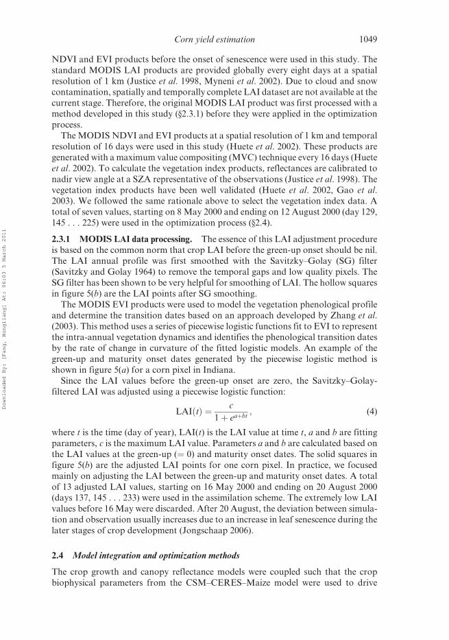
NDVI and EVI products before the onset of senescence were used in this study. The

standard MODIS LAI products are provided globally every eight days at a spatial

resolution of 1 km (Justice et al. 1998, Myneni et al. 2002). Due to cloud and snow

contamination, spatially and temporally complete LAI dataset are not available at the

current stage. Therefore, the original MODIS LAI product was first processed with amethod developed in this study (§2.3.1) before they were applied in the optimization

process.

The MODIS NDVI and EVI products at a spatial resolution of 1 km and temporal

resolution of 16 days were used in this study (Huete et al. 2002). These products are

generated with a maximum value compositing (MVC) technique every 16 days (Huete

et al. 2002). To calculate the vegetation index products, reflectances are calibrated to

nadir view angle at a SZA representative of the observations (Justice et al. 1998). The

vegetation index products have been well validated (Huete et al. 2002, Gao et al.2003). We followed the same rationale above to select the vegetation index data. A

total of seven values, starting on 8 May 2000 and ending on 12 August 2000 (day 129,

145 . . . 225) were used in the optimization process (§2.4).

2.3.1 MODIS LAI data processing. The essence of this LAI adjustment procedureis based on the common norm that crop LAI before the green-up onset should be nil.

The LAI annual profile was first smoothed with the Savitzky–Golay (SG) filter

(Savitzky and Golay 1964) to remove the temporal gaps and low quality pixels. The

SG filter has been shown to be very helpful for smoothing of LAI. The hollow squares

in figure 5(b) are the LAI points after SG smoothing.

The MODIS EVI products were used to model the vegetation phenological profile

and determine the transition dates based on an approach developed by Zhang et al.

(2003). This method uses a series of piecewise logistic functions fit to EVI to representthe intra-annual vegetation dynamics and identifies the phenological transition dates

by the rate of change in curvature of the fitted logistic models. An example of the

green-up and maturity onset dates generated by the piecewise logistic method is

shown in figure 5(a) for a corn pixel in Indiana.

Since the LAI values before the green-up onset are zero, the Savitzky–Golay-

filtered LAI was adjusted using a piecewise logistic function:

LAI tð Þ ¼ c

1þ eaþbt; (4)

where t is the time (day of year), LAI(t) is the LAI value at time t, a and b are fitting

parameters, c is the maximum LAI value. Parameters a and b are calculated based on

the LAI values at the green-up (¼ 0) and maturity onset dates. The solid squares in

figure 5(b) are the adjusted LAI points for one corn pixel. In practice, we focused

mainly on adjusting the LAI between the green-up and maturity onset dates. A total

of 13 adjusted LAI values, starting on 16 May 2000 and ending on 20 August 2000(days 137, 145 . . . 233) were used in the assimilation scheme. The extremely low LAI

values before 16 May were discarded. After 20 August, the deviation between simula-

tion and observation usually increases due to an increase in leaf senescence during the

later stages of crop development (Jongschaap 2006).

2.4 Model integration and optimization methods

The crop growth and canopy reflectance models were coupled such that the crop

biophysical parameters from the CSM–CERES–Maize model were used to drive



the Markov model. A general form of cost function J was constructed as (Liang

2004):

J X t0ð Þð Þ ¼ X t0ð Þ � Xb½ �T B�1 X t0ð Þ � Xb½ �

þXn

i¼1

Hi X tið Þð Þ � Yi½ �T R�1i Hi X tið Þð Þ � Yi½ �; (5)

where Xb is the background value (or first guess), X(t0) and X(ti) are the observed

values at time t0 and ti, respectively, H is the crop model operator and Yi are the

observations. R and B are the observation and background error covariance matrices,

respectively, and were set as unity here.

The cost function was based on the differences between the simulated and

measured LAI using the conjugate direction optimization algorithm POWELL

provided by Press et al. (1992). This method efficiently minimizes computingtime and was used in this study. A simplified minimization was applied here to

calculate the cost functions:

Figure 5. (a) A sample time-series of MODIS EVI data and the estimated phenologicaltransition dates for a corn pixel in Indiana, 2000. (b) The original MODIS LAI (cross), theLAI after the SG filter (hollow square) and the adjusted LAI (solid square) based on thephenological dates from (a) and a piecewise logistic function in equation (4).

1050 H. Fang et al.


J1 ¼Xm

i¼1

abs LAIð ÞS tið Þ � LAIð ÞM tið Þ� �

= LAIð ÞM tið Þ (6)

J2 ¼Xn

j¼1

abs VIð ÞS tj

� �� VIð ÞM tj

� �� = VIð ÞM tj

� �(7)

J3 ¼1

m

Xm

i¼1

abs LAIð ÞS tið Þ � LAIð ÞM tið Þ� �

= LAIð ÞM tið Þ

þ 1

n

Xn

j¼1

abs VIð ÞS tj

� �� VIð ÞM tj

� �� = VIð ÞM tj

� �; (8)

where LAIS(ti), LAIM(ti) are the simulated and measured LAI at time ti, respectively;

VIS, VIM are the simulated and measured Vegetation Indices, respectively; m and n are

the number of LAI and vegetation index values.

The optimization process starts from an initial parametrization and adjusts the free

parameters in the coupled crop yield and radiative transfer model in order that the

model gives LAI and/or vegetation index simulation in agreement with the MODIS

observations. Table 3 shows an example of a typical optimization process for one

pixel. The last column is the cost function calculated at different iterations based onequations (6), (7) and (8). Six model variables, four for the CSM–CERES–Maize

(planting date, plant population, row spacing and nitrogen fertilizer amount) and two

Table 3. Adjustment of the free parameters in the optimization process.

No.iteration

Plantingdate

(DOY)Planting

population

Rowspacing

(cm)

Nitrogenamount(kgha-1)

Soil redreflectance

Leafstructure

Costfunction

(J)

1 128 6.5 80 44 0.1 1.8 2.922 128 6.5 80 44 0.1 1.8 2.923 128 6.5 80 44 0.1 1.8 2.924 128.6 6.5 80 44 0.1 1.8 2.925 129.6 6.5 80 44 0.1 1.8 2.556 131.1 6.5 80 44 0.1 1.8 2.4222 130 6.5 80 44 0.1 1.8 2.5523 130 6.6 80 44 0.1 1.8 2.5524 130 6.6 80 44 0.1 1.8 2.5525 130 6.7 80 44 0.1 1.8 2.5526 130 6.9 80 44 0.1 1.8 2.5527 130 7.2 80 44 0.1 1.8 2.5528 130 7.5 80 44 0.1 1.8 59731.6129 130 7.2 80 44 0.1 1.8 2.5530 130 7.3 80 44 0.1 1.8 2.55385 157.5 7.5 90 56.9 0.5 3 0.84386 157.5 7.5 90 56.9 0.5 3 0.84387 157.5 7.5 90 56.9 0.5 3 0.84Optimized

value157.5 7.5 90 56.9 0.5 3 0.84

The parameters are adjusted sequentially based on the cost function J value. Planting date is thefirst parameter to be adjusted (rows in iterations 1–6), followed by the planting population(rows in iterations 22–30) and others. The last row shows the final optimized value.



for the Markov model (red band soil reflectance and the effective number of elemen-

tary layers in a leaf) were adjusted and optimized sequentially based on the cost

function. The last row shows the resultant optimized values for that pixel when the

maximum number of iterations or the minimum merit function is achieved.

The simulated LAI or vegetation index values depend on the values of the freevariables (e.g. planting date, see table 1) that are estimated by minimizing the cost

function J. To compare the effect of using different control variables, five schemes

were designed: S1 (LAI), S2 (EVI), S3 (NDVI), S4 (EVIþLAI) and S5 (NDVIþLAI).

The first scheme was similar to our earlier work using LAI as the control variable

(Fang et al. 2008), but different free variables were applied in this study. The cost

function equations (6), (7), and (8) were applied for schemes S1, S2 and S3, and S4 and

S5, respectively.

3. Results

The model was run on a daily time step for each corn pixel (1 km) in Indiana in 2000.

Only pixels that had more than 80% corn were treated as ‘pure’ corn pixels and were

processed with this methodology. In total, 871 ‘pure’ corn pixels were identified in

2000 (Fang et al. 2008) based on the USDA cropland data layer (CDL) (http://

www.nass.usda.gov/research/Cropland/SARS1a.htm).

3.1 Crop yield

A comparison of the estimated corn yield and NASS yield data for selected counties in

Indiana, 2000 is presented in figure 6. USDA NASS has developed methods to assess

crop growth and development from various sources of information, including several

types of surveys of farm operators. NASS provides monthly projected estimates ofcrop yield and production. For the estimated yield, a total of 43 counties contains

valid yield data by having at least 5 km2 planted in corn (�5 pixels) within the county.

The results from the five schemes are shown. The dashed line indicates the mean

absolute bias between the estimated and measured yields. The best results are based

on schemes with both vegetation index and LAI (S4 and S5), which have the lowest

root mean square errors (RMSEs) and biases. When only vegetation index is used

(S2 and S3), the results are unacceptable. Using only LAI (S1) generates moderately

good results. Comparing the distribution of the estimated and NASS yields for allcounties in 2000, the NASS county yields are mostly clustered between 8000 kg ha-1

and 10 500 kg ha-1, while the simulated yield scatters between 5000 kg ha-1 and

15 000 kg ha-1. The yield distribution of schemes S1, S4 and S5 is comparable to that

of the NASS data, while the mean values of S2 and S3 are higher and lower,

respectively, than the NASS data.

Table 4 compares the statistics obtained from the estimated and NASS yields. The

best results are obtained from S5 using NDVIþLAI, with an estimated yield that is

only 0.2% lower than the NASS data. The corn yield from S4 (EVIþLAI) gives verygood results and the relative difference is 3.5%. In contrast, the results from S2 and S3

differ greatly from the measurements. The standard deviations from the estimated

results are all higher than those of the NASS data. The schemes with only EVI or

NDVI perform poorly. Scheme S2 (EVI) and S3 (NDVI) show the largest over-

estimation (20.8%) and underestimation (–13.2%), respectively. This phenomenon

indicates the importance of LAI in the data assimilation process and that the incor-

poration of both LAI and vegetation index can improve crop yield prediction.

1052 H. Fang et al.


Figure 7 shows the spatial distribution of corn yield for different schemes on 11 July2000 (Julian day 193). The corn yield was generated for 871 corn pixels in the state. It

is clear that corn was grown mainly in the central counties of the state. The magnitude

and spatial distribution in general agree with the NASS statistics. The Ohio River

valley has the highest planting density and corn yield compared to other regions. The

yield distributions of S4 and S5 are comparable to S1. For S2 and S3, discrepancies are

seen in the eastern and northern parts of the state. The greatest deviation between the

predicted and measured yields occurs for S2 (EVI only), which overestimates the corn

yield, although the spatial pattern is in reasonable agreement with the observed

Table 4. Comparison of the estimated corn yield and NASS data in Indiana, 2000 (kg ha-1).

Estimated yields based on different schemes

NASS data S1 (%) S2 (%) S3 (%) S4 (%) S5 (%)

Mean 9080 9857 8.6 10967

20.8 7885 -13.2 9396 3.5 9060 -0.2

STD* 700 1228 2468 873 1405 1015

Estimated yields are from five different schemes: S1 (LAI), S2 (EVI), S3 (NDVI), S4 (EVIþLAI)and S5 (NDVIþLAI). Their relative differences (%) with the NASS yield are also shown.*STD, standard deviation.

Figure 6. Comparison of the estimated corn yield and USDA NASS yield data for selectedcounties (43) in Indiana, 2000: (a) S1 (LAI); (b) S2 (EVI); (c) S3 (NDVI); (d) S4 (EVIþLAI);(e) S5 (NDVIþLAI). The abscissa and ordinate are the estimated and measured corn yield(kg ha-1), respectively. The dashed line shows the mean offset indicated by ‘Diff’. RMSE, rootmean square error.



values. In contrast, using NDVI only underestimates the corn yield, whereas its

spatial pattern is quite similar to that when using EVI.

Using the adjusted LAI leads to an improved yield estimation when compared with a

previous study using the original MODIS LAI (Fang et al. 2008). The mean difference

in crop yield between the estimated and NASS decreased from 685 kg ha-1 using the

Figure 7. Spatial distribution of the estimated corn yields for Indiana, 2000 with five differentschemes: (a) S1 (LAI); (b) S2 (EVI); (c) S3 (NDVI); (d) S4 (EVIþLAI); (e) S5 (NDVIþLAI).Unit: Kg ha-1

1054 H. Fang et al.


MODIS LAI to 395 kg ha-1 using the adjusted LAI. This indicates that the adjusted

LAI could better characterize the crop growth status in the study area. Considering the

uncertainties in the MODIS LAI products and in the coupled model, this level of yield

agreement is very satisfying. In general, results from S1, S4 and S5 agree with the NASS

data. Using both vegetation index and LAI demonstrated the best results.

3.2 LAI estimated through data assimilation methods

The current MODIS LAI products suffer from two problems: cloud contamination

and temporal discontinuity (Myneni et al. 2002). The purpose of an eight-day com-

posite is to eliminate cloud contamination, but it remains an issue in current MODIS

LAI products (Myneni et al. 2002). Moreover, some studies require LAI with a higher

temporal resolution. For example, Kang et al. (2003) used a linear interpolation todownscale from eight-day LAI to a daily unit for a greenness onset study.

Interpolation and other mathematical fitting methods, while filling in missing days,

would eventually change reliable values.

Although use of the MODIS daily surface reflectance could provide LAI at a daily

time step, this advantage is constrained by daily cloud contamination and increased

computing loads. Moreover, surface reflectance or its derivative (e.g. VIs) does not

always correspond to an identical LAI value, but shows a statistical distribution that

depends on the canopy physiological status (Myneni et al. 2002). In contrast, cropgrowth models can estimate LAI when no remote sensing products are available,

especially during the early growth and senescence periods. Thus, it is feasible to

monitor LAI and crop conditions all along the phenological cycle instead of only

from isolated snapshot images.

The simulated mean LAI values from the five schemes are illustrated in figure 8.

For comparison, the mean values of the MODIS LAI, the Savitzky–Golay-filtered

LAI and the adjusted LAI are also displayed. All five schemes generate similar LAI

values and profiles. In the CSM–CERES–Maize model, the estimation of LAI isbased on the transformed dry matter from the absorbed solar energy, and the

distribution of biomass among leaves, stems and roots. LAI relates mainly to the

carbon balance in the crop simulation process and is more affected by crop type and

weather conditions. In the re-initialization process for free variables, the simulated

LAI values were automatically recalculated in the CSM–CERES–Maize model to fit

the observed ones. Once the free variables are optimized, the simulated LAI profiles

are similar among the different assimilation schemes (figure 8).

The seasonal phenology of the LAI is properly simulated by the model (figure 8). Themodelled LAI and adjusted LAI match very well during the peak growing season and after

maturity.ThesimulatedLAIiswithinthestandarddeviationoftheadjustedLAI(figure8).

Some deviations are evident during the green-up period. The seven-day difference (137,

145 ... 185) ranges from -0.09 to 0.95 and has a mean deviation of 0.31 between the

simulated (S1) and adjusted LAI. However, the mean difference between the original

MODIS LAI and simulated LAI (S1) ranges from 0.29 to 0.92, with a mean of 0.64. This

phenomenon can be explained mostly by the obvious overestimation of the MODIS LAI

products during the green-up period (Cohen et al. 2003, Fang and Liang 2005). This alsoreveals that the adjusted LAI could describe the crop growth status very well. The variation

of both the MODIS LAI and the adjusted LAI is greater than that of the modelled LAI.

With the method developed in this study, we were able to generate a daily LAI map

for the state of Indiana. Figure 9 displays the MODIS LAI product, the adjusted



Figure 8. The simulated mean LAI for Indiana from the five schemes, 2000. Also shown arethe original MODIS LAI (cross), the LAI after SG filtering (hollow square) and the adjustedLAI based on the piecewise logistic function (solid square). The segments are the standarddeviation of the adjusted LAI over the state.

Figure 9. Comparison of (a) the MODIS LAI, (b) the adjusted MODIS LAI and (c) thesimulated LAI from S4 (EVIþLAI) on day 193, 2000.

1056 H. Fang et al.


MODIS LAI and the simulated LAI from S4 (EVIþLAI) on 11 July 2000 (DOY 193).

The MODIS LAI product shows mixed LAI values evenly distributed across the state

in July. Both the adjusted and simulated LAI values show a decreasing gradient

between 1.0 and 2.0 from the west toward the east. Figure 10 shows the probability

density of the modelled and MODIS LAI for the same day. For comparison, thetemporally adjusted LAI is also displayed in figure 10. The adjusted LAI shows a very

similar probability density as the MODIS LAI because of good observations for this

eight-day period (figure 10). Visually, the adjusted LAI (figure 9(b)) is smoother than

the original MODIS LAI (figure 9(a)) because the adjusted LAI enhances the low-

LAI pixels (, 1) in central and southern Indiana and reduces some higher LAI pixels

(. 6). The MODIS LAI shows a distribution plateau around 4.0–5.0. In contrast, the

simulated LAI is concentrated around 2,4, with a peak at 3.0 (figures 9(c) and 10).

Unlike the simulated LAI, the MODIS LAI values spread between 0 and 6. This isunderstandable because of the differences in algorithms, estimation assumptions and

pixel unmixing methods.

3.3 Vegetation indices

Figure 11 shows the temporal profile of the simulated mean EVI (a) and NDVI (b) for

the entire study area. For comparison, the state of Indiana’s mean MODIS EVI and

NDVI are also shown with dots (mean) and line segments (standard deviation).

Figure 12 compares the probability density of the modelled and MODIS vegetation

indices on 11 July 2000 (DOY 193).Seven vegetation index values from the green-up to the peak growth period are

compared (figure 11). After day 225, the vegetation index decreases. For the study

period, the simulated EVI is lower than the NDVI. This is also observed for the

MODIS vegetation index products. The highest simulated EVI and NDVI are

observed at 0.68 and 0.90 for days 193 and 209, respectively (figure 11). Both S2

and S4 provide EVI as an intermediate variable. It is noted that the two EVI profiles

from the two schemes are nearly identical (figure 11(a)). Likewise, S3 and S5 provided

Figure 10. Comparison of the probability densities of the MODIS LAI, the adjusted LAI andthe simulated LAI from S4 (EVIþLAI) on day 193, 2000.



very similar NDVI profiles (figure 11(b)). Among the seven days, the simulated

vegetation indices agree very well with the MODIS vegetation index for the lastfour days (177, 193, 209 and 225). For three other days (129, 145 and 161), the

MODIS vegetation index is higher than the simulated vegetation index. For these

three days, the average deviations between the modelled and observed vegetation

indices are 0.248 for EVI and 0.254 for NDVI, respectively. Like the MODIS LAI, the

MODIS vegetation index values before emergence (e.g. day 129) may have a large

variation resulting from a mixture of crop and soil at the surface (Huete et al. 2002).

The standard deviation of the MODIS vegetation index is higher than those of the

simulated ones, indicating that the MODIS vegetation index is more variable forIndiana. This is also illustrated by the probability density graph in figure 12.

The spatial distribution of the simulated EVI agree with the MODIS EVI except

for a few isolated higher values (. 0.9). The same phenomenon is observed for the

modelled NDVI and MODIS NDVI. The range of the simulated values is very

similar to that of the observed ones, although the latter is more scattered. The

simulated EVI distribution peak is at 0.724, compared to 0.714 for MODIS EVI

(figure 12). For the simulated NDVI, there is a density peak at around 0.897, higher

than that of the MODIS NDVI (0.857). The distribution of the MODIS vegetationindex is more similar to a normal distribution, while the modelled ones are more

clustered.

4. Discussion

4.1 Practical application of the data assimilation approach

With the coupled crop growth and canopy reflectance model, the seasonal corn yield

was successfully estimated with only a partial year of remotely sensed data before

senescence onset. In this study, MODIS LAI before 20 August 2000 (day 233) and

vegetation index data before 12 August 2000 (day 225) were used to predict the end-

of-season corn yield. In the study area, corn harvest usually happens from late

September to early November. Spatial distribution information about crop yield

Figure 11. The simulated seasonal VIs for Indiana, 2000: (a) EVI from S2 and S4; (b) NDVIfrom S3 and S5. The points and segments are the mean and standard deviation of the MODISEVI (a) and NDVI (b) products over the state.

1058 H. Fang et al.


was also obtained by this method. The data assimilation approach has great potential

for operational corn yield estimation for other seasons.

One of our goals is to compare the effect of using LAI and vegetation index in data

assimilation. The results indicate that LAI showed moderately good results while best

results were obtained when both LAI and vegetation indices were used as the control

variables. Using only NDVI significantly underestimated the corn yield while usingonly EVI over-predicted the yield. The inefficiency of using a vegetation index may be

attributed to uncertainties in the radiative transfer model and the spatial variation of

the MODIS products. Both schemes using NDVI (S3 and S5) predicted lower yields

than those with EVI (S2 and S4). This might be due to soil background reflectance

since it is not fully accounted for by NDVI.

In this study, daily LAI and vegetation index were generated through the

CSM–CERES–Maize model. The MODIS LAI and vegetation index products

reproduced the natural variation of the crop phenology satisfactorily. A new LAIadjustment method was developed to calibrate the original MODIS LAI based on

the vegetation phenological information derived from the MODIS EVI product.

The new LAI series consists of the adjusted LAI from the piecewise logistic function

before maturity and the original MODIS LAI after maturity. The adjusted LAI

proved to be very useful for the data assimilation study. When compared to using

the original MODIS LAI, using the adjusted LAI data improved the corn yield

estimation. Upon full validation, the simulated daily LAI and vegetation index data

can complement the current MODIS products.

Figure 12. Comparison of the probability densities of the MODIS EVI and NDVI productswith that of the simulated EVI and NDVI from S2 (EVI) and S3 (NDVI), respectively, on day193, 2000.



4.2 Uncertainties and challenges

There are several sources of uncertainty in the estimation of crop yield. For example,

we assumed optimal growing and management conditions. However, management

factors (e.g. a cultivar’s genetic characteristics and use of fertilizers) and exceptional

events (pests or flooding) will affect the predicted yield observed in farmers’ fields. It is

important to evaluate the model performance under high-yield conditions, as well as

in environments that produce lower-yield levels under stress conditions to ensure a

comprehensive assessment of model performance (Yang et al. 2004). USDA NASS

yield statistics are designed to provide very accurate estimates at the state level, whilein the assimilation model county-level yields are estimated and adjusted to sum to the

state level. Note that these results are based on pixels at a 1 km resolution, while

statistical yields are based on administrative regions.

The assimilation model would certainly benefit from better parametrization of the

radiative transfer model. In this study, we fixed several parameters, such as canopy

architecture, and leaf and soil optical properties. Better results may be obtainable with

the use of more accurate parameter estimation for the leaf chlorophyll content, the

total amount of equivalent water and dry matter (protein, cellulose and lignin). Theymay be obtained from the remote sensing methods separately and applied in the data

assimilation process. For example, leaf chlorophyll content can be retrieved from high

resolution remote sensing imagery (Fang et al. 2003). The leaf water content can be

estimated from MODIS data through a radiative transfer model inversion method

(Zarco-Tejada et al. 2003).

Potential uncertainties in the remotely sensed products need to be noted in such a

data assimilation study. Some further improvements of the MODIS-derived LAI and

vegetation index products are necessary, especially during the beginning of the grow-ing season. This is also revealed in other similar studies (Adiku et al. 2006). In our

study, the simulated LAI and vegetation index seasonal profiles showed that the

MODIS LAI, EVI and NDVI products overestimated during the beginning of the

season by about 0.64, 0.25 and 0.25, respectively.

Six model variables (table 1), four for the CSM–CERES–Maize model (planting

date, plant population, row spacing and nitrogen fertilizer amount) and two for the

Markov model (red band soil reflectance and the effective number of elementary

layers in a leaf), were selected as free variables based on a series of sensitivity analyses.Different variable selection would affect the results. Since we focus on comparing the

application of LAI and vegetation indices in the data assimilation process, a detailed

sensitivity analysis considering other parameters should be performed in subsequent

studies.

5. Conclusion

In this study, a data assimilation method was developed to estimate crop yield at the

regional scale by assimilating MODIS LAI and vegetation index products into acoupled model consisting of the CSM–CERES–Maize crop growth model and the

Markov canopy reflectance model. The assimilation method automatically tunes a set

of input parameters until the difference between the MODIS LAI and vegetation

index products and those simulated by the model is minimized. The final corn yield is

estimated with the optimized input data.

By assimilating only a partial year of remotely sensed data we could effectively

predict the seasonal crop yield one or two months before harvest. The estimated corn

1060 H. Fang et al.


yield over Indiana in 2000 agreed very well with the corn yield obtained from NASS

statistics, both in spatial distribution as well as for the yield levels. The best results were

obtained with a relative deviation less than 3.5% when both the LAI and EVI or NDVI

were assimilated. When only one vegetation index was used, the bias was larger than

13%. Compared with using only LAI or only a vegetation index, a synergic use of LAIand vegetation index data makes the assimilated model more responsive to changes in

the crop biophysical characters. The spatial variation of crop yield was found to be

related to the scattering of the MODIS LAI and vegetation index products. With a

proper model setting, the assimilation method described in this work is very promising

for forecasting the long-term yield for other crop types in a larger region.

The soil, weather and crop parameter datasets developed for this study could

provide useful guidelines for model applications in other regions. Several further

studies can be foreseen. Regional hydrological information can be estimated by theassimilation approach in this study. Alternative optimization algorithms could be

explored considering their computational efficiency and accuracy. Similar studies can

be carried out for a different set of agricultural environment and canopy character-

istics. More rigorous evaluation is necessary to investigate the model efficiency for

various climatic and atmospheric conditions.

Acknowledgements

This work was supported by US Department of Agriculture (USDA) grant SCA58-

1275-9-096. The authors would like to thank Dr Xiaoyang Zhang, Earth Resources

Technology, Inc. for providing the phenology code. The daily weather data were

distributed by the North America Land Data Assimilation Systems (NLDAS),

located at the Goddard Space Flight Center, NASA (http://ldas.gsfc.nasa.gov/).

ReferencesABOU-ISMAIL, O., HUANG, J. and WANG, R., 2004, Rice yield estimation by integrating remote

sensing with rice growth simulation model. Pedosphere, 14, pp. 519–526.

ADIKU, S.G.K., REICHSTEIN, M., LOHILA, A., DINH, N.Q., AURELA, M., LAURILA, T., LUEERS, J.

and TENHUNEN, J.D., 2006, PIXGRO: A model for simulating the ecosystem CO2

exchange and growth of spring barley. Ecological Modeling, 190, pp. 260–276.

ASADI, M.E. and CLEMENTE, R.S., 2001, Simulation of maize yield and N uptake under

tropical conditions with the CERES–Maize model. Tropical Agriculture, 78, pp.

211–217.

BACH, H., MAUSER, W. and SCHNEIDER, K., 2003, The use of radiative transfer models for

remote sensing data assimilation in crop growth models. In Precision Agriculture:

Papers from the 4th European Conference on Precision Agriculture, 15–19 June 2003,

Berlin, Germany, J. Stafford and A. Werner (Eds), pp. 35–40 (Wageninger, The

Netherlands: Wageninger Academic Publishers).

BACH, H., SCHNEIDER, K., VERHOEF, W., STOLZ, R., MAUSER, W., LEEUWEN, H., SCHOUTEN, L.

and BORGEAUD, M., 2001, Retrieval of geo- and biophysical information from remote

sensing through advanced combination of a land surface process model with inversion

techniques in the optical and microwave spectral range. In 8th International Symposium

Physical Measurements & Signatures in Remote Sensing, pp. 639–647 (France: Centre

Paul Langevin, Aussois).

BARET, F., WEISS, M., TROUFLEAU, D., PREVOT, L. and COMBAL, B., 2000, Maximum informa-

tion exploitation for canopy characterisation by remote sensing. Aspects of Applied

Biology, 60, pp. 71–82.



BOOGAARD, H.L., DIEPEN, C.A.V., ROTTER, R.P., CABRERA, J.M.C.A. and LAAR, H.H.V., 1998,

WOFOST 7.1; User’s Guide for the WOFOST 7.1 Crop Growth Simulation Model and

MOFOST Control Center 1.5 (Wageningen: DLO Winand Staring Centre).

BOUMAN, B.A.M., 1992, Linking physical remote sensing models with crop growth simulation

models, applied for sugar beet. International Journal of Remote Sensing, 13, pp. 2565–2581.

BULLOCK, D.G. and ANDERSON, D.S., 1998, Evaluation of the Minolta SPAD-502 chlorophyll

meter for nitrogen management in corn. Journal of Plant Nutrition, 21, pp. 741–755.

CLEVERS, J.G.P.W., BUKER, C., LEEUWEN, H.J.C.V. and BOUMAN, B.A.M., 1994, A framework

for monitoring crop growth by combining directional and spectral remote sensing

information. Remote Sensing of Environment, 50, pp. 161–170.

COHEN, W.B., MAIERSPERGER, T.K., YANG, Z., GOWER, S.T., TURNER, D.P., RITTS, W.D.,

BERTERRETCHE, M. and RUNNING, S.W., 2003, Comparisons of land cover and LAI

estimates derived from ETMþ and MODIS for four sites in North America: a quality

assessment of 2000/2001 provisional MODIS products. Remote Sensing of

Environment, 88, pp. 233–255.

DAUGHTRY, C.S., 2001, Discriminating crop residues from soil by shortware infrared reflec-

tance. Agronomy Journal, 93, pp. 125–131.

DAVIS, L., 1991, Handbook of Genetic Algorithms (New York: Van Nostrand Reinhold).

DELECOLLE, R., MAAS, S.J., GUERIF, M. and BARET, F., 1992, Remote sensing and crop

production models: present trends. ISPRS Journal of Photogrammetry and Remote

Sensing, 47, pp. 145–161.

DENTE, L., SATALINO, G., MATTIA, F. and RINALDI, M., 2008, Assimilation of leaf area index

derived from ASAR and MERIS data into CERES–Wheat model to map wheat yield.

Remote Sensing of Environment, 112, pp. 1395–1407.

DE WIT, A.J.W., 1999, The application of a genetic algorithm for crop model steering using

NOAA–AVHRR data. In Proceedings of SPIE Vol. 3868, E. Zilioli, E.T. Engman and

G. Cecchi (Eds), pp. 167–181 (Bellingham, WA: SPIE).

DORAISWAMY, P.C., HATFIELD, J.L., JACKSON, T.J., AKHMEDOV, B., PRUEGER, J. and STERN, A.,

2004, Crop condition and yield simulation using Landsat and MODIS. Remote Sensing

of Environment, 92, pp. 548–559.

DORAISWAMY, P.C., MOULIN, S., COOK, P.W. and STERN, A., 2003, Crop yield assessment from

remote sensing. Photogrammetric Engineering and Remote Sensing, 69, pp. 665–674.

FANG, H. and LIANG, S., 2003, Retrieve LAI from Landsat 7 ETMþ data with a neural network

method: Simulation and validation study. IEEE Transactions on Geoscience and

Remote Sensing, 41, pp. 2052–2062.

FANG, H. and LIANG, S., 2005, A hybrid inversion method for mapping leaf area index from

MODIS data: Experiments and application to broadleaf and needleleaf canopies.


FANG, H., LIANG, S., HOOGENBOOM, G., TEASDALE, J. and CAVIGELLI, M., 2008, Corn yield

estimation through assimilation of remote sensed data into the CSM–CERES–Maize

model. International Journal of Remote Sensing, 29, pp. 3011–3032.

FANG, H., LIANG, S. and KUUSK, A., 2003, Retrieving leaf area index using a genetic algorithm

with a canopy radiative transfer model. Remote Sensing of Environment, 85, pp.

257–270.

GAO, X., HUETE, A.R. and DIDAN, K., 2003, Multisensor comparisons and validation of

MODIS vegetation indices at the semiarid Jornada Experimental Range. IEEE

Transactions on Geoscience and Remote Sensing, 41, pp. 2368–2381.

GOLDBERG, D.E., 1989, Genetic Algorithms in Search, Optimization and Machine Learning

(Reading, MA: Addison-Wesley).

GUERIF, M. and DUKE, C.L., 2000, Adjustment procedures of a crop model to the site specific

characteristics of soil and crop using remote sensing data assimilation. Agriculture,

Ecosystems & Environment, 81, pp. 57–69.

1062 H. Fang et al.


HOOGENBOOM, G., JONES, J.W., WILKENS, P.W., PORTER, C.H., BATCHELOR, W.D., HUNT, L.A.,

BOOTE, K.J., SINGH, U., URYASEV, O., BOWEN, W.T., GIJSMAN, A.J., TOIT, A.D., WHITE,

J.W. and TSUJI, G.Y., 2004, Decision Support System for Agrotechnology Transfer

Version 4.0 [CD-ROM] (Honolulu, Hawaii: University of Hawaii).

HOOGENBOOM, G., WILKENS, P.W. and TSUJI, G.Y. (Eds), 1999, Decision Support System for

Agrotechnology Transfer, Version 3 Volume 4 (Honolulu, Hawaii: University of Hawaii).

HUETE, A., DIDAN, K., MIURA, T., RODRIGUEZ, E.P., GAO, X. and FERREIRA, L.G., 2002,

Overview of the radiometric and biophysical performance of the MODIS vegetation

indices. Remote Sensing of Environment, 83, pp. 195–213.

JACQUEMOUD, S., BACOUR, C., POILVE, H. and FRANGI, J.P., 2000, Comparison of four radiative

transfer models to simulate plant canopies reflectance-direct and inverse mode. Remote

Sensing of Environment, 74, pp. 471–481.

JACQUEMOUD, S. and BARET, F., 1990, PROSPECT: a model of leaf optical properties spectra.


JACQUEMOUD, S., USTIN, S.L., VERDEBOUT, J., SCHMUCK, G., ANDREOLI, G. and HOSGOOD, B.,

1996, Estimating leaf biochemistry using the PROSPECT leaf optical properties model.


JET PROPULSION LABORATORY (JPL), 1998, Aster Spectral Library, Version 1.2 (Pasadena, CA:

Jet Propulsion Laboratory). Available online at http://speclib.jpl.nasa.gov.

JIANG, D., WANG, N.B., YANG, X.H. and WANG, J.H., 2003, Study on the interaction between

NDVI profile and the growing status of crops. Chinese Geographical Science, 13,

pp. 62–65.

JONES, J.W., HOOGENBOOM, G., PORTER, C.H., BOOTE, K.J., BATCHELOR, W.D., HUNT, L.A.,

WILKENS, P.W., SINGH, U., GIJSMAN, A.J. and RITCHIE, J.T., 2003, The DSSAT crop-

ping system model. European Journal of Agronomy, 18, pp. 235–265.

JONGSCHAAP, R.E.E., 2006, Run-time calibration of simulation models by integrating remote

sensing estimates of leaf area index and canopy nitrogen. European Journal of

Agronomy, 24, pp. 316–324.

JUSTICE, C.O., VERMOTE, E., TOWNSHEND, J.R.G., DEFRIES, R., ROY, D.P., HALL, D.K.,

SALOMONSON, V.V., PRIVETTE, J.L., RIGGS, G., STRAHLER, A., LUCHT, W., MYNENI,

R.B., KNYAZIKHIN, Y., RUNNING, S.W., NEMANI, R.R., WAN, Z., HUETE, A.R. and

VAN LEEUWEN, W., 1998, The Moderate Resolution Imaging Spectroradiometer

(MODIS): land remote sensing for global change research. IEEE Transactions on

Geoscience and Remote Sensing, 36, pp. 1228–1249.

KANG, S., RUNNING, S.W., LIM, J.-H., ZHAO, M., PARK, C.-R. and LOEHMAN, R., 2003, A

regional phenology model for detecting onset of greenness in temperate mixed forests,

Korea: an application of MODIS leaf area index. Remote Sensing of Environment, 86,

pp. 232–242.

KIMES, D.S., KNYAZIKHIN, Y., PRIVETTE, J.L., ABUELGASIM, A.A. and GAO, F., 2000, Inversion

methods for physically-based models. Remote Sensing Review, 18, pp. 381–440.

KINIRY, J.R., WILLIAMS, J.R., VANDERLIP, R.L., ATWOOD, J.D., REICOSKY, D.C., MULLIKEN, J.,

COX, W.J., MASCAGNI, H.J.J., HOLLINGER, S.E. and WIEBOLD, W.J., 1997, Evaluation of

two maize models for nine U.S. locations. Agronomy Journal, 89, pp. 421–426.

KOGAN, F., YANG, B., GUO, W., PEI, Z. and JIAO, X., 2005, Modelling corn production in China

using AVHRR-based vegetation health indices. International Journal of Remote

Sensing, 26, pp. 2325–2336.

KUUSK, A., 1998, Monitoring of vegetation parameters on large areas by the inversion of a

canopy reflectance model. International Journal of Remote Sensing, 19, pp. 2893–2905.

KUUSK, A., 2001, A two-layer canopy reflectance model. Journal of Quantitative Spectroscopy

and Radiative Transfer, 71, pp. 1–9.

KUUSK, A., ANDRIEU, B., CHELLE, M. and ARIES, F., 1997, Validation of a Markov chain canopy

reflectance model. International Journal of Remote Sensing, 18, pp. 2125–2146.

LIANG, S., 2004, Quantitative Remote Sensing of Land Surfaces (New York: John Wiley and Sons).



LIANG, S. and QIN, J., 2008, Data assimilation methods for land surface variable estimation. In

Advances in Land Remote Sensing: System, Modeling, Inversion and Application, S.

Liang (Ed.), pp. 319–339 (New York: Springer).

LIZASO, J.I., BATCHELOR, W.D. and ADAMS, S.S., 2001, Alternate approach to improve kernel

number calculation in CERES–maize. Transactions of the ASAE, 44, pp. 1011–1018.

MAAS, S., 1988a, Using satellite data to improve model estimates of crop yield. Agronomy

Journal, 80, pp. 662–665.

MAAS, S.J., 1988b, Use of remotely-sensed information in agricultural crop growth models.

Ecological Modeling, 41, pp. 247–268.

MACDONALD, R. and HALL, F., 1980, Global crop forecasting. Science, 208, pp. 670–679.

MO, X., XIANG, Y., MCVICAR, T.R., LIU, S., LIN, Z. and XU, Y., 2005, Prediction of crop yield,

water consumption and water use efficiency with a SVAT-crop growth model using

remotely sensed data on the North China Plain. Ecological Modeling, 183, pp. 301–322.

MOULIN, S., BONDEAU, A. and DELECOLLE, R., 1998, Combining agricultural crop models and

satellite observations: from field to regional scale. International Journal of Remote

Sensing, 19, pp. 1021–1036.

MYNENI, R.B., HOFFMAN, S., KNYAZIKHIN, Y., PRIVETTE, J.L., GLASSY, J., TIAN, Y., WANG, Y.,

SONG, X., ZHANG, Y., SMITH, G.R., LOTSCH, A., FRIEDL, M., MORISETTE, J.T., VOTAVA,

P., NEMANI, R.R. and RUNNING, S.W., 2002, Global products of vegetation leaf area

and fraction absorbed PAR from year one of MODIS data. Remote Sensing of


O’NEAL, M.R., FRANKENBERGER, J.R. and ESS, D.R., 2002, Use of CERES–Maize to study

effect of spatial precipitation variability on yield. Agricultural Systems, 73, pp. 205–225.

PLUMMER, S.E., 2000, Perspectives on combining ecological process models and remotely

sensed data. Ecological Modeling, 129, pp. 169–186.

PRESS, W.H., TEUKOLSKY, S.A., VETTERLING, W.T. and FLANNERY, B.P., 1992, Numerical

Recipes in Fortran 77: The Art of Scientific Computing (New York: Cambridge

University Press).

PRICE, J.C., 1990, On the information content of soil reflectance spectra. Remote Sensing of


QIN, J., LIANG, S., LI, X. and WANG, J., 2008, Development of the adjoint model of a canopy

radiative transfer model for sensitivity study and inversion of leaf area index. IEEE

Transactions on Geoscience and Remote Sensing, 46, pp. 2028–2037.

SAVITZKY, A. and GOLAY, M.J.E., 1964, Smoothing and differentiation of data by simplified

least squares procedures. Analytical Chemistry, 36, pp. 1627–1639.

SINGH, R., GOYAL, R.C., SAHA, S.K. and CHHIKARA, R.S., 1992, Use of satellite spectral data in

crop yield estimation surveys. International Journal of Remote Sensing, 14, pp.

2583–2592.

THENKABAIL, P.S., WARD, A.D., LYON, J.G. and VAN DEVENTER, P., 1992, Landsat Thematic

Mapper indices for evaluating management and growth characteristics of soybeans and

corn. Transactions of the ASAE, 35, pp. 1441–1448.

TOJO SOLER, C.M., SENTELHAS, P.C. and HOOGENBOOM, G., 2007, Application of the

CSM–CERES–Maize model for planting date evaluation and yield forecasting for

maize grown off-season in a subtropical environment. European Journal of

Agronomy, 27, pp. 165–177.

TSUJI, G.Y., UEHARA, G. and BALAS, S., 1994, Decision Support System for Agrotechnology

Transfer, Version 3 (Honolulu, Hawaii: University of Hawaii).

TUBIELLO, F.N., ROSENZWEIG, C., KIMBALL, B.A., PINTER, P.J.J., WALL, G.W., HUNSAKER, D.J.,

LAMORTE, R.L. and GARCIA, R.L., 1999, Testing CERES–wheat with free-air carbon

dioxide enrichment (FACE) experiment data: CO2 and water interactions. Agronomy

Journal, 91, pp. 247–255.

WEISS, M., TROUFLEAU, D., BARET, F., CHAUKI, H., PREVOT, L., OLIOSO, A., BRUGUIER, N. and

BRISSON, N., 2001, Coupling canopy functioning and radiative transfer models for

1064 H. Fang et al.


remote sensing data assimilation. Agricultural and Forest Meteorology, 108, pp.

113–128.

WEISSTEINER, C.J. and KUHBAUCH, W., 2005, Regional yield forecasts of malting barley

(Hordeum vulgare L.) by NOAA–AVHRR remote sensing data and ancillary data.

Journal of Agronomy and Crop Science, 191, pp. 308–320.

XIE, Y., KINIRY, J.R., NEDBALEK, V. and ROSENTHAL, W.D., 2001, Maize and sorghum simula-

tions with CERES–maize, SORKAM, and ALMANAC under water-limiting condi-

tions. Agronomy Journal, 93, pp. 1148–1155.

YANG, H.S., DOBERMANN, A., LINDQUIST, J.L., WALTERS, D.T., ARKEBAUER, T.J. and CASSMAN,

K.G., 2004, Hybrid–maize – a maize simulation model that combines two crop model-

ing approaches. Field Crops Research, 87, pp. 131–154.

ZARCO-TEJADA, P.J., RUEDA, C.A. and USTIN, S.L., 2003, Water content estimation in vegeta-

tion with MODIS reflectance data and model inversion methods. Remote Sensing of


ZHANG, X., FRIEDL, M.A., SCHAAF, C.B., STRAHLER, A.H., HODGES, J., GAO, F., REED, B. and

HUETE, A., 2003, Monitoring vegetation phenology using MODIS. Remote Sensing of




International Journal of Remote Sensing Integration of ...

Documents

Transcript of International Journal of Remote Sensing Integration of ...