Internally Contracted Multireference Coupled Cluster Theory.

Computer Aided Implementation of

Advanced Electronic Structure Methods.

Marcel Nooijen Chemistry Department University of Waterloo nooijen@uwaterloo.ca

Summary

In the past decade efficient Coupled Cluster methods have been developed to obtain accurate results for electronically excited states, e.g. Equation-of-Motion CC (EOMCC) / CC Linear Response Theory (CCLRT) / SAC-CI, Fock Space CC and Similarity Transformed EOMCC (STEOM-CC). All of these methods can be characterized as "Transform & Diagonalize, T&D" approaches: Single reference techniques are used to extract a transformation of the Hamiltonian that incorporates dynamical correlation effects. The transformed Hamiltonian is subsequently diagonalized over a compact subspace to obtain the states of interest. The focus of the talk will be on a generalization of the T&D concepts to genuine multireference situations. This leads to an efficient formulation of a state selective internally contracted multireference CC theory and I will present some applications to medium sized systems. Although the methodology is efficient, it is also rather complicated. We developed an automation tool, the Automatic Program Generator (APG), that allows us to derive, factorize and implement equations in an effective way. The APG has been invaluable to develop our current multireference coupled cluster strategy, as it allowed us to explore quickly a large number of variations on the theme.

Basic Strategy: "Transform then Diagonalize".

Transform: G U HU= −1 - Transformation U should account for short-range,

dynamical, electron correlation effects. - Can be expected to work for multiple states at once, if

they are in some sense similar. - Transformation does not change eigenvalues.

Diagonalize: GC C= E

- Choose U such that C can be compact. Truncated diagonalization space / selection of configurations.

Advantages: - Access to wave function. - Multiple states may be treated at once → balance. - Approach is in principle exact, independent of U . Disadvantages: - Selection of diagonalization space (active space) will

depend on user. Unlikely to be completely black box. - Transformation U is in principle arbitrary. How to find

something that is useful in practice?

Internally Contracted MRCC Theory

Basic form for the wave function

Ψ = +e S RT ( )1 0

0 : Closed shell determinant (vacuum in MB theory).

R 0 : Reference state → qualitatively correct wfn.

T T T= +1 2 excitation operators w.r.t. 0 (q-creation).

S S S= +1 2 : S 0 0= , but SR 0 0≠ . (q-annihilation). - Spin- and -symmetry adaptation: T and S have

same symmetry as for closed shell case (generators of unitary group).

- Size-consistency: eT suffices (because S 0 0= ) - Internally Contracted: ,T S act as an entity on

reference state → relatively few parameters. - State selective: Coefficients will be determined for

one state at a time (or a few states in a state averaged formulation).

Define ( )1 0+ = → =S R C e CTΨ

Schrödinger equation : He C Ee CT T0 0=

e He C HC ECT T− = =0 0 0

Akin to Equation of Motion CC Theory.

In EOM-CC eT 0 itself is approximate eigenstate Here T (and 0 ) are specific for state of interest.

Define left-hand zeroth-order eigenstate 0 L

0 0 0 0 0La e He C La C Eijab T T

ijab− = = → T2

Φ Φλ λ λe He C E C EcT T− = =0 0 → C

Equation for single excitations ??

What is 0 ??

Is C particle conserving ??

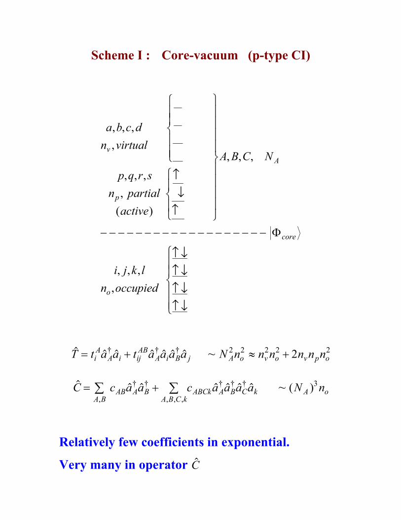
Scheme I : Core-vacuum (p-type CI)

a b c dn virtual

p q r sn partial

active

A B C N

i j k ln occupied

v

p

A

core

o

, , ,,

, , ,,

( )

, , ,

, , ,,

RS||

T||ABA

RS|T|

U

V

||||

W

||||− − − − − − − − − − − − − − − − − − −

ABABABAB

RS||

T||

Φ

† † †T t a a t a a a aiA

A i ijAB

A i B j= + ~ N n n n n n nA o v o v p o2 2 2 2 22≈ +

,

† †

, , ,

† † †C c a a c a a a aA B

AB A BA B C k

ABCk A B C k= +∑ ∑ ~ ( )N nA o3

Relatively few coefficients in exponential.

Very many in operator C

Scheme II: Full Vacuum (h-type CI)

a b c dn virtual

p q r sn partial

active

i j k ln occupied

I J K N

v

full

p

o

I

, , ,,

, , ,,

( )

, , ,,

, , ,

RS||

T||

− − − − − − − − − − − − − − − − − − −

ABA

RS|T|ABABABAB

RS||

T||

U

V

||||

W

||||

Φ

† † †T t a a t a a a aI

aa I IJ

aba I b J= + ~ n N n n n n nv I v o o p v

2 2 2 2 22≈ +

†C c a a c a a a aIJ I J IJcK I J c K= + ~ N nI v3

Many coefficients in exponential operator T . Relatively few in operator C

Scheme III: half filled vacuum (# of electrons).

ph-type CI

-

a b c dn virtual

p q r sn partial

A B C N

active

i j k ln occupied

I J K N

v

p

A

o

I

, , ,,

, , ,,

, , ,

( )

, , ,,

, , ,

RS||

T||BARST

U

V

||||

W

||||− − − − − − − − − − − − − − − − − − −

AABABABAB

RS||

T||

U

V|||

W|||

Φ0

m

† † †T t a a t a a a aIA

A I IJAB

A I B J= + ~ n N n n n n nA I v o o v p2 2 2 2 22≈ +

C same form as T + higher rank excitation ops.

Complicated scheme. Not further pursued.

Most favorable scheme: hole-type CI. - Doubly occupy all orbitals that are strongly

occupied in the full wave function (" user's selection"). This specifies the vacuum state 0 having 2 N I electrons.

- The operator C would consist of nh and (n+1)h-1p

type of excitation operators. The number of electrons in the state of interest is 2 N I - n Nel= .

- Typical example: systems with one low lying

virtual orbital → increase the number of electrons by two → 0 .

,

†C c a a C a a a aI J

IJ I JI J K c

IJcK I J c K= +< < <∑ ∑

State Selective DIP-MRCC scheme.

In principle applicable to

Biradicals

Breaking of single bonds Twisting of double bonds

Many photo-chemical reactions

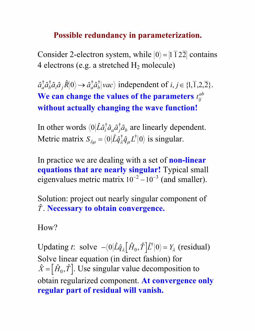
Possible redundancy in parameterization.

Consider 2-electron system, while 0 11 22= contains 4 electrons (e.g. a stretched H2 molecule)

† † † †a a a a R a a vaca b i j a b0 → independent of i j, { , , , }∈ 1 1 2 2 . We can change the values of the parameters tij

ab without actually changing the wave function! In other words 0 † †La a a ai a j b are linearly dependent. Metric matrix S Lq q Lλµ λ µ= 0 0† † is singular. In practice we are dealing with a set of non-linear equations that are nearly singular! Typical small eigenvalues metric matrix 10 102 3− −− (and smaller). Solution: project out nearly singular component of T . Necessary to obtain convergence. How? Updating t: solve − =0 00, †Lq H T L Yλ λ (residual) Solve linear equation (in direct fashion) for

,X H T= 0 . Use singular value decomposition to obtain regularized component. At convergence only regular part of residual will vanish.

Size consistency

Consider non-interacting subsystems

A ................................ B Open-shell Closed Shell orbitals i, a Orbitals j, b

E=EA+EB

The open-shell problem (operator C) should be completely localized on system A. If we assume that H has localized matrix elements then the additional condition is Φ j

bjbH h0 0= = . (for excitations on B).

Relevant Matrix structure of H

exc. ij ijck ijck

ij X X X ijck X X X ijck 0 ! 0 X

If C is localized on A then equations reduce to CCSD for system B. 0 0 0 0 02 2LQ HC Q H→ = where Q2 indicates excitation on system B. Results are size-consistent provided ...

Equations for single excitations are crucial: Possibilities: 1. ΦK

cKcH h0 0= = ??

Typically leads to large singles and poor results. 0 is not Hartree-Fock determinant for N+2 electrons. 2. 0 0 0†La a HCK b = ?? These equations are completely redundant (!) as 0 †La aK b is 3h1p excitation. T1 0= would be solution.

Violates size-consistency (because ill defined). 3. 0 0 0† †La a HLK b = Good, size-consistent results. Small singles coefficients.

Formulation of n-hole type MCSCF:

0 0 01 1† †La a e He LK bT T− =

Solve eqns. in Brueckner fashion and use T1 as orbital rotation parameters → variationally optimal 0 that we use in practice. Closed-shell orbital optimization.

Algorithm to solve MRCC equations. 1. Solve Brueckner MCSCF equations → L 0 Variant A. Full MRCC scheme: iterate

a. Calculate relevant parts of H e HeT T= − b. Solve IP-/ EA-/ DIP-EOM-CC eqns → C c. Factorize (approximately) C SC2 10 0= → S d. Calculate residuals 0 1 02 1( )LQ H S C+ and 0 01 1LQ HC (Coded by APG) e. Find regularized updates for ,T T1 2

Variant B. State-Selective (ST)EOM-CC Iteratively solve 0 02

†LQ HL = 0 01†LQ HL =0

(Coded by APG) Calculate H e HeT T= − Solve IP-/ EA-/ DIP-EOMCC or STEOM equations.

Illustrations Redundancy / Projection.

Consider H2 molecule at stretched geometry Ψ ≈ +c cg g u uσ σ2 2

At R=1.5 Å in TZ2P basis c cg u= = −0 947 0 322. , .

Various exact solutions to the problem using different projections 0 L

Projection used t g u( )σ π2 2→ t u u( )σ π2 2→ c cg g u uσ σ2 2+ -0.034 0.011

σ g2 -0.037 0

σ u2 0 0.118

O2: Vacuum state in MRCC is 0 4 4= ....π πu g . Low lying excited states π g

−2 but mixing with π u−2.

Results depend slightly upon projection used:

Method 3Σu,− 1∆ g 1Σ g,+ Re (Å) ω (cm-1) E (a.u.) ∆ (eV) ∆ (eV)MRDIP 1.214 1571 -150.0785 0.991 1.596

t-MRDIP 1.207 1634 -150.0728 1.034 1.640

CCSD 1.207 1631 -150.0723 -- --

CCSD(T) 1.220 1540 -150.0895

Solving for the t-amplitudes: In every iteration calculate residuals Q Qi

aijab,

Solve − =0 00,†R e H T R Qij

abijab

- Equations can be (nearly) singular - Not fully dominant on diagonal → special singular value decomposition solver.

What is †H p ppp

0 = ∑ε ?

Amplitudes tij

ab correspond to excitation from (partially) occupied orbitals into virtual orbitals:

- ε i : ionization potentials obtained using extended Koopmans' Theorem (EKT).

- Diagonalize ( )H E− 0 over states i R i0 →ε : Completely different (~ 20 eV) from diagonalizing Fock matrix !

- εa: Electron affinities corresponding to EKT. - Diagonalize ( )H E− 0 over states †a R a0 →ε . :

Equivalent to diagonalizing Fock matrix.

Is the Algorithm numerically stable ??

Severe test: Calculate vibrational frequencies of twisted ethylene in lowest singlet and triplet state.

Symmetry of molecule and character of orbitals changes as finite displacements are made to calculate Hessian.

Triplet State Singlet State

CCSD MRCC STEOM MRCC STEOM RCC 1.475 1.477 1.479 1.475 1.478 RCH 1.093 1.094 1.091 1.096 1.094

< HCC 121.4 121.3 121.2 121.5 121.5

ω 1 (E) 318 322 311 416 449

ω 2 (B1) 666 667 666 1887 i 1756 i

ω 3 (E) 948 948 952 960 968

ω 4 (A1) 1135 1129 1126 1132 1121

ω 5 (A1) 1456 1454 1464 1455 1461

ω 6 (B2) 1490 1488 1496 1486 1490

ω 7 (A1) 3156 3152 3187 3124 3136

ω 8 (B2) 3157 3153 3191 3130 3144

ω 9 (E) 3256 3252 3305 3218 3250

H

H

H

H

Accuracy of MRCC, SS-EOMCC and STEOM compared to CCSD and CCSD(T).

Consider singlet and triplet in ethylene at D2h and D2d

geometries (barrier to bond rotation).

Method D2d D2d Barrier D2h triplet

total E ST-spitting D2d(T)-

D2h(S) ST-splitting

(a.u.) (kcal/mol) (kcal/mol) (eV)

MRCC -78.3305 1.35 67.91 4.379SS-DIPEOM -78.3335 0.93 (1.24*) 68.18 4.414

DIPEOM -78.3078 0.65 74.35 4.687SS-STEOM -78.317 2.12 71.98 4.639

STEOM -78.326 1.69 60.92 4.153CCSD -78.3302 64.68 4.238

CCSD(T) -78.3400 67.38 4.381

Method D2d D2d Barrier D2h triplet

total E ST-spitting D2d(T)-

D2h(S) ST-splitting

(a.u.) (kcal/mol) (kcal/mol) (eV)

DIP-STEOM [2-] -78.2715 2.03 63.4 104.4DIP-EOM [2-] -78.2765 0.60 67.8 101.8

SS-DIPEOM [mb] -78.2802 1.13 66.2 103.3SS-DIPEOM [R] -78.2837 0.83 65.4 102.4

CCSD -78.2811 -20.47 83.5 98.6

CCSD[T] -78.2875 -4.42 69.6 101.3

- For triplet states (spin-adapted) MRCC results are

virtually identical to ROHF-CCSD. - MRCC is well balanced: both barrier and ST-splitting

at D2h geometry compare well to CCSD(T). - STEOM and DIPEOM energetics not very accurate

for larger basis sets due to use of di-anion orbitals in the reference state.

The Benzynes

Method para-benzyne meta-benzyne ortho-benzyne T S-T T - T(p) S-T T - T(p) S-T total E

(a.u.) (kcal) (kcal) (kcal) (kcal) (kcal

) MRCC -230.1892 4.38 4.08 16.8 4.3 33.8

B-MRCC -230.1873 3.97 4.08 16.5 4.8 34.4SS-DIPEOM -230.1906 4.24 11.17 25.2 19.1 46.3

STEOM -230.1789 5.66 1.37 14.0 10.8 31.5

CCSD -230.1882 -16.90 1.04 (2.96) 5.8 (6.5) 4.1 27.8CCSD(T) -230.2227 4.58 1.21 (3.72) 16.5 (17.8) 4.0 32.8

- In general good agreement between MRCC based

on MCSCF orbitals and full Brueckner MRCC. - Meta-benzyne is difficult system, e.g. large

difference between ROHF- and UHF-CCSD(T). - Poor results for SS-DIPEOM : large difference

between relaxed C1 and MCSCF R1.

p-benzyne m-benzyne o-benzyne

S-T splitting in Methylene CH2

TZ2P basis, MBPT[2] geometries.

MRCC SS-DIPEOM STEOM CCSD CCSD(T) 11.55 12.58 14.11 12.40 11.52

Comparisons with Full CI results.

H4 ground state

Geom. FCI B-MRCC B-SS-DIPEOM

B-MRCC relaxed

CCSDT

Total E (H) ∆E in mH 0.01 -2.0694 -0.006 0.31 -0.003 -1.020.05 -2.1143 0.082 0.92 0.08 -0.070.10 -2.16012 0.45 0.75 0.43 -0.020.15 -2.18893 0.34 0.79 0.33 -0.020.50 -2.2327 0.21 0.55 0.18 -0.02

H4 First Excited State

Geom. FCI B-

MRCC B-SS-

DIPEOM B-MRCC relaxed

Total E (H) ∆E in mH 0.01 -1.98064 0.38 1.43 0.38 0.05 -1.94450 0.28 1.59 0.28 0.10 -1.90089 0.24 2.09 0.22 0.15 -1.87719 0.27 3.31 0.25 0.50 -1.86511 0.28 2.71 0.29

H8 ground and excited state

FCI B-MRCC B-SS-DIPEOM

B-MRCC Relaxed

STEOM

Ground State (∆E in mH) 0.01 -4.30836 4.39 10.54 1.22 -0.600.1 -4.31581 4.40 6.71 1.43 -1.431.0 -4.41654 1.99 6.03 1.77 -1.74

First Excited State (∆E in mH) 0.01 -4.25737 2.05 2.30 2.09 -4.450.1 -4.25260 3.02 3.07 2.65 -4.561.0 -4.09485 17.07 19.96 18.11 11.00

Computer Aided Development of Electronic Structure Programs

Dr. Victor Lotrich and M. Nooijen

Why? - New tools needed to tackle resilient problems

in quantum chemistry. - Such tools tend to be highly complex, but are

not necessarily computationally expensive.

- The 'right' tools are not known yet. Experimentation is necessary.

- Current strategies: prone to errors, tedious,

labor intensive, repetitive, not pedagogical for students.

- Efficiency, robustness and applicability of

programs can be increased.

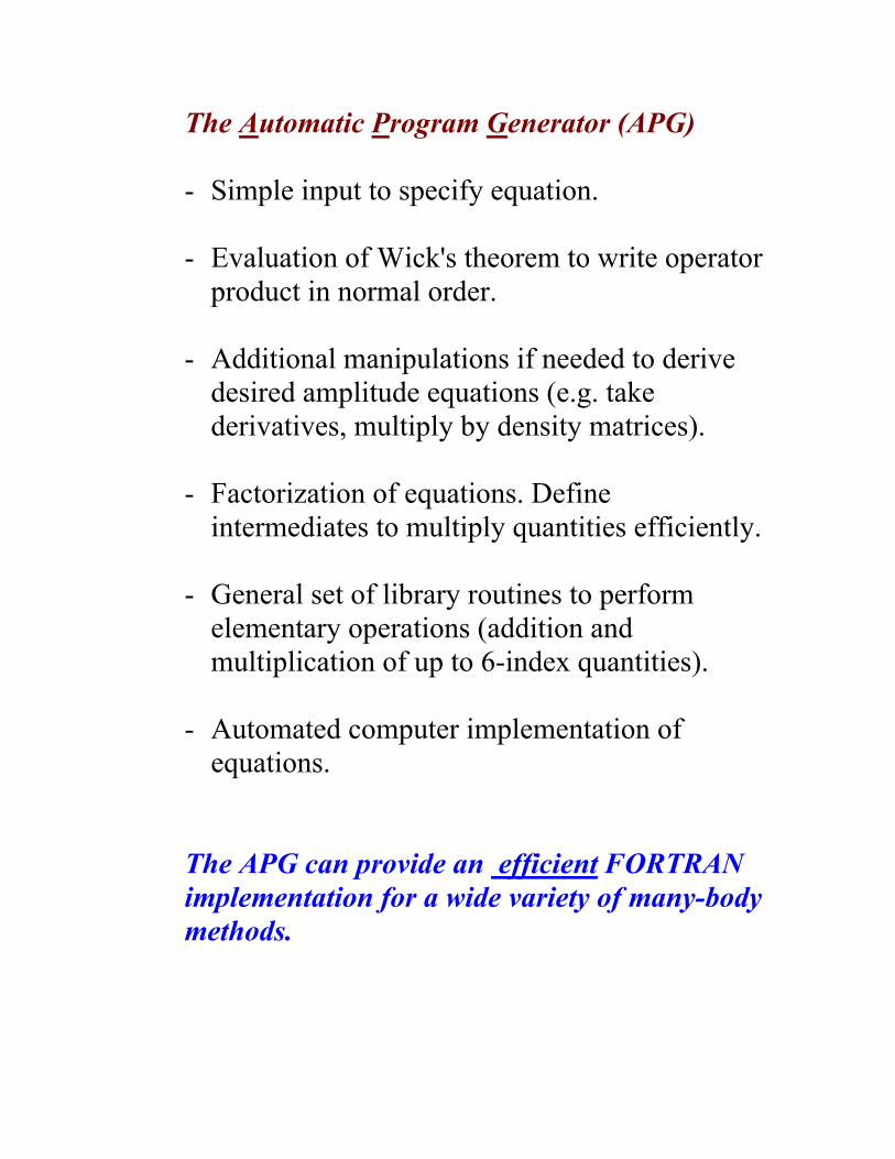
The Automatic Program Generator (APG) - Simple input to specify equation. - Evaluation of Wick's theorem to write operator

product in normal order.

- Additional manipulations if needed to derive desired amplitude equations (e.g. take derivatives, multiply by density matrices).

- Factorization of equations. Define

intermediates to multiply quantities efficiently.

- General set of library routines to perform elementary operations (addition and multiplication of up to 6-index quantities).

- Automated computer implementation of

equations.

The APG can provide an efficient FORTRAN implementation for a wide variety of many-body methods.

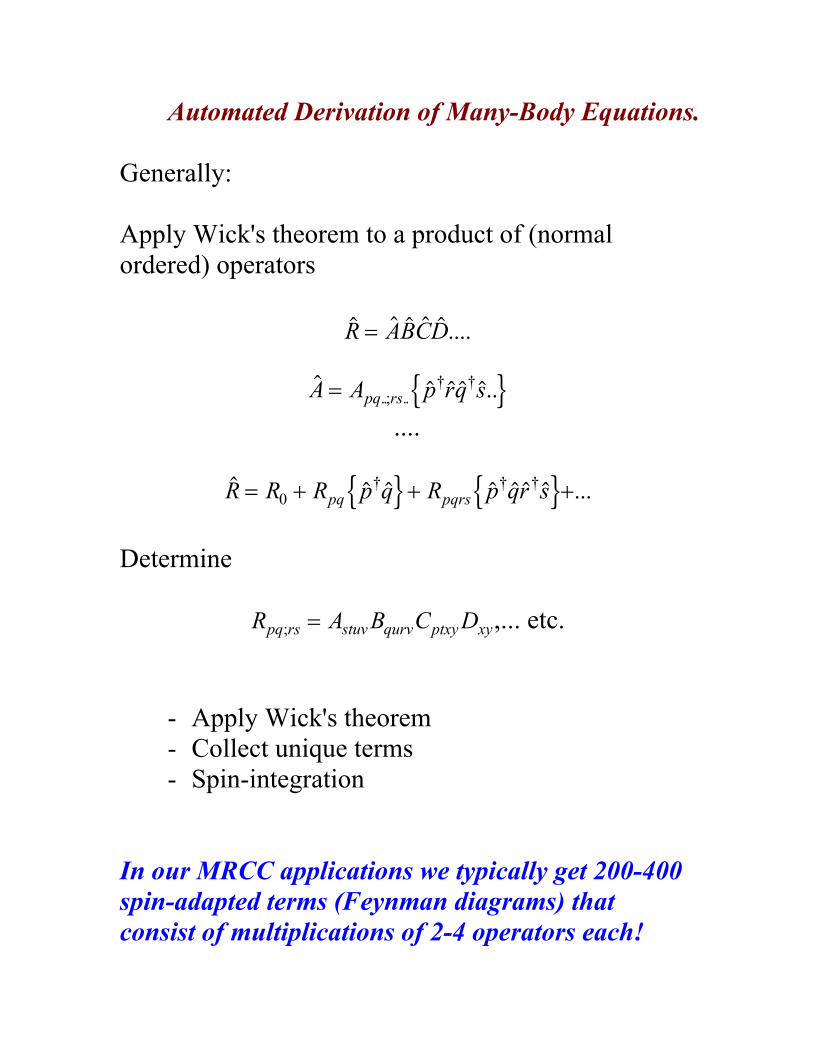
Automated Derivation of Many-Body Equations. Generally: Apply Wick's theorem to a product of (normal ordered) operators ....R ABCD= ....; ..

† †A A p rq spq rs= n s .... ...† † †R R R p q R p qr spq pqrs= + + +0 n s n s Determine R A B C Dpq rs stuv qurv ptxy xy; = ,... etc.

- Apply Wick's theorem - Collect unique terms - Spin-integration

In our MRCC applications we typically get 200-400 spin-adapted terms (Feynman diagrams) that consist of multiplications of 2-4 operators each!

Factorization

Use only 2 elementary operations to sum all terms. Addition: A B Cpqrs pqrs pqrs= + Matrix-Multiplication. A B C Dpq rs pq rs pq tu tu rs; ; ; ;= + Split up general term

R A B C D n

I A B n

I C D n

R I I n

pq rs stuv qurv ptxy xy

st qr stuv qurv

pt pt xy xy

pq rs st qr pt

;

;

;

; ;

=

→

=

=

=

9

1 6

2 4

1 2 5

Intermediates need to be stored and might be (partially) reused to evaluate other terms. Definition of intermediates effects operation count and storage costs. Optimal factorization consitutes n-p complete problem in mathematics. Typically there may be 10200 (!) different ways to factorize.

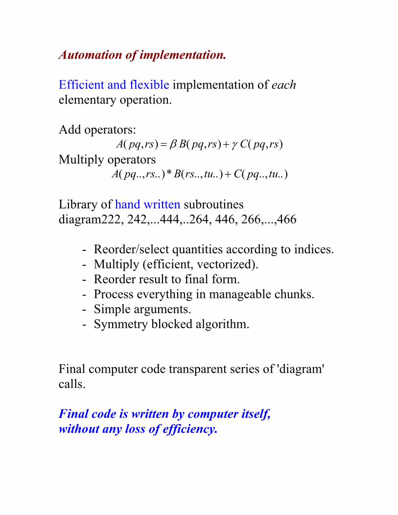
Automation of implementation. Efficient and flexible implementation of each elementary operation. Add operators: A pq rs B pq rs C pq rs( , ) ( , ) ( , )= +β γ Multiply operators A pq rs B rs tu C pq tu( .., ..)* ( .., ..) ( .., ..)+ Library of hand written subroutines diagram222, 242,...444,..264, 446, 266,...,466

- Reorder/select quantities according to indices. - Multiply (efficient, vectorized). - Reorder result to final form. - Process everything in manageable chunks. - Simple arguments. - Symmetry blocked algorithm.

Final computer code transparent series of 'diagram' calls. Final code is written by computer itself, without any loss of efficiency.

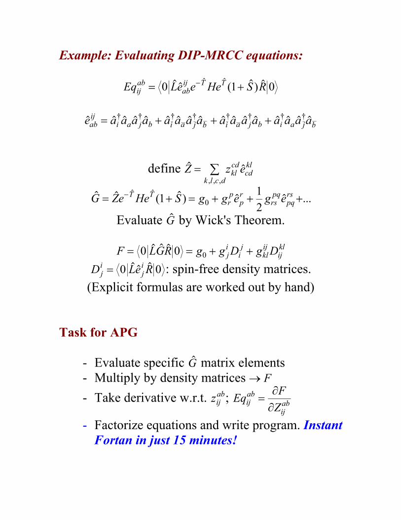
Example: Evaluating DIP-MRCC equations:

Eq Le e He S Rijab

abij T T= +−0 1 0( )

† † † † † † † †e a a a a a a a a a a a a a a a aab

iji a j b i a j b i a j b i a j b= + + +

define , , ,

Z z ek l c d

klcd

cdkl= ∑

( ) ...G Ze He S g g e g eT Trp

pr

rspq

pqrs= + = + + +− 1 1

20

Evaluate G by Wick's Theorem.

F LGR g g D g Dji

ij

klij

ijkl= = + +0 0 0

D Le Rji

ji= 0 0 : spin-free density matrices.

(Explicit formulas are worked out by hand) Task for APG

- Evaluate specific G matrix elements - Multiply by density matrices → F - Take derivative w.r.t. zij

ab; Eq FZij

ab

ijab=

∂∂

- Factorize equations and write program. Instant Fortan in just 15 minutes!

Summary:

- State-Selective Equation-of-Motion Coupled Cluster. - Transform then Diagonalize approach to general open-

shell problems. - Equations for transformation coefficients t fairly

insentitive to details. - Suitable zeroth-order Hamiltonian using "Extended

Koopmans Theorem. + Perturbation Theory. - General Equations with o2v4 scaling.

!! Computer Aided Implementations !!

Work in Progress: "Tensor Contraction Engine"

Computer generated implementations.

Optimize traffic of data flow Cache ↔ Ram ↔Disk↔Recomputation.

Sadayappan, Baumgartner, Harrison, Hirata,

Corciova, Bernholdt, Pitzer, Nooijen