1

Interim Analysis in Clinical Trials

Professor Bikas K Sinha [ ISI, KolkatA ]Courtesy : Dr Gajendra Viswakarma

Visiting ScientistIndian Statistical Institute

Tezpur Centree-mail: sinhabikas@yahoo.com

2

What is a clinical trial?

A test of a new intervention or treatment on people for detecting

-Tolerability

-Safety

-Efficacy

A Clinical trial is defined as a prospective study comparing the effect and value of intervention (s) against a control in human beings.

3

Types of clinical trials

Superiority

Non-inferiority

Equivalence

It can be a Phase I, Phase II or Phase III Trial

4

Diagrammatical Presentation of Clinical Trials

Control better Test better- 0

equivalence

non-inferior

superior

5

Clinical Trial Stages

Phase I: Clinical Pharmacology and Toxicity

Objective: To determine a safe drug dose for further studies of therapeutic efficacy of the drug

Design: Dose-escalation to establish a maximum tolerated dose (MTD) for a new drug

Subjects: 1-10 normal volunteers or patients with disease

6

Clinical Trial Stages

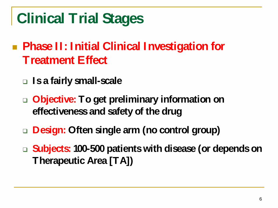
Phase II: Initial Clinical Investigation for Treatment Effect

Is a fairly small-scale

Objective: To get preliminary information on effectiveness and safety of the drug

Design: Often single arm (no control group)

Subjects: 100-500 patients with disease (or depends on Therapeutic Area [TA])

7

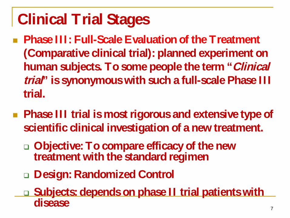
Clinical Trial StagesPhase III: Full-Scale Evaluation of the Treatment (Comparative clinical trial): planned experiment on human subjects. To some people the term “Clinical trial” is synonymous with such a full-scale Phase III trial.

Phase III trial is most rigorous and extensive type of scientific clinical investigation of a new treatment.

Objective: To compare efficacy of the new treatment with the standard regimenDesign: Randomized ControlSubjects: depends on phase II trial patients with disease

8

Clinical Trial Stages

Phase IV: Post-Marketing

After the research program leading to a drug being approved for marketing, there remain substantial inquiries still to be undertaken as regards monitoring for adverse effects and additional large-scale, long-term studies of morbidity and mortality.

Objective: To get more information (long-term side effects)

Design: no control group

Subjects: Patients with disease using the treatment

9

The Big Picture

DRUG A DRUG B

Test stat

10

… So What is Different?

Ethics: Experiment involving human subjects brings up new ethical issuesBias: Experiment on intelligent subjects requires new measures of control

We will also study the additional considerations in clinical trials

to address the above requirements.

11

Interim Analysis

Analysis comparing intervention groups at any time before the formal completion of the trial, usually before recruitment is complete.

Often used with "stopping rules" so that a trial can be stopped if participants are being put at risk unnecessarily.

Timing and frequency of interim analyses should be specified in the protocol.

12

Interim Analyses

Interim analyses is a tool to protect the welfare of subjects

By stopping enrollment/treatment as soon as a drug is determined to be harmfulBy stopping enrollment as soon as a drug is determined to be highly beneficialBy stopping trials which will yield little additional useful information (or which have negligible chance of demonstrating efficacy if fully enrolled, given results to date)

The associated statistical methods are generally referred to as group sequential methods

13

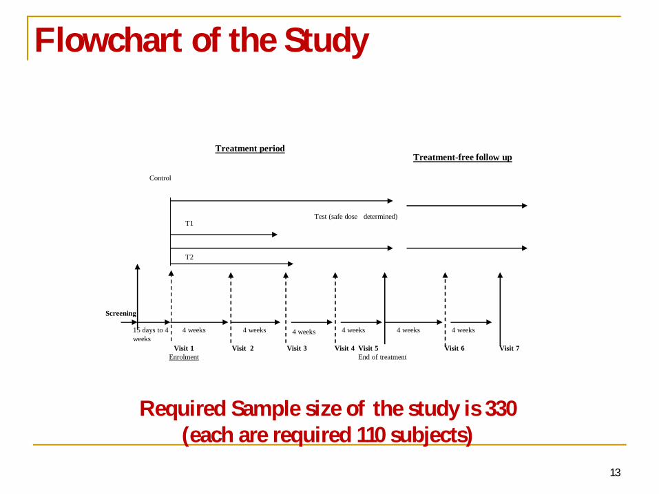
Flowchart of the Study

Visit 6

T2

T1

Visit 5End of treatment

Visit 4

Control

Visit 1Enrolment

Visit 2 Visit 3

15 days to 4 weeks

4 weeks 4 weeks 4 weeks

Treatment-free follow upTreatment period

4 weeks 4 weeks

Screening

Test (safe dose determined)

Visit 7

4 weeks

Required Sample size of the study is 330 (each are required 110 subjects)

14

Disposition Table on going study

Drug C Drug T1 Drug T2 Total

Patient Screened 129

Screening Failure 23

Patient Randomized 36 36 34 106

Study Incomplete + ongoing 9+5 8+5 10+3 28+12

Completed Visits 5+ 22 23 21 66

15

Mean PASI Change at Visits in Different Treatment Groups

0.00

2.00

4.00

6.00

8.00

10.00

12.00

14.00

16.00

V1 V2 V3 V4 V5

Visit

Mea

n PA

SIDrug A Drug B Drug C

16

Some Examples of Why a Trial May Be Terminated

Treatments found to be convincingly differentTreatments found to be convincingly not differentSide effects or toxicities are too severeData quality is poorAccrual is slowDefinitive information becomes available from an outside source making trial unnecessary or unethicalScientific question is no longer importantAdherence to treatment is unacceptably lowResources to perform study are lost or diminishedStudy integrity has been undermined by fraud or misconduct

17

Opposing Pressures in Interim Analyses

To Terminate:minimize size of trialminimize number of patients on inferior armcosts and economicstimeliness of results

To Continue:increase precisionreduce errorsincrease powerincrease ability to look at subgroupsgather information on secondary endpoints

18

The pitfalls of interim analyses

RCTs [Randomized Clinical Trials] with interim analysis

1. Calculate sample size2. Carry out the clinical trial3. Employ statistical test of efficacy at pre-planned

stages in the interim until sample size has been reached*

*One treatment declared significantly better than the other if we get a p-value less than 5%.....

19

Statistical Considerations in Interim Analyses

Consider a safety/efficacy study (phase II)“At this point in time, is there statistical evidence that….”

The treatment will not be as efficacious as we would hope/need it to be?The treatment is clearly dangerous/unsafe?The treatment is very efficacious and we should proceed to a comparative trial?

20

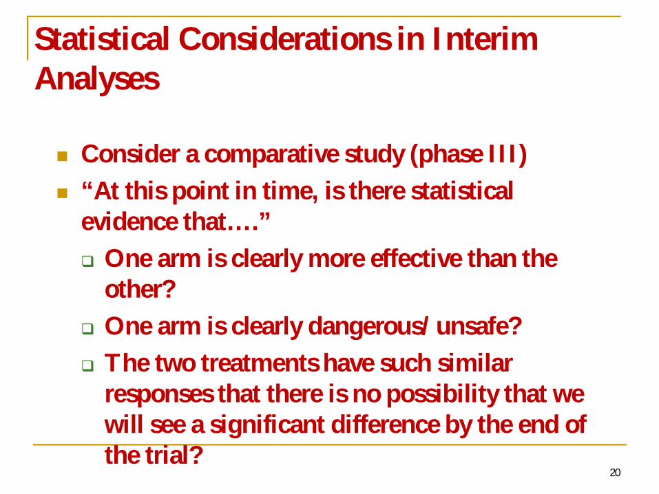
Consider a comparative study (phase III)“At this point in time, is there statistical evidence that….”

One arm is clearly more effective than the other?One arm is clearly dangerous/unsafe?The two treatments have such similar responses that there is no possibility that we will see a significant difference by the end of the trial?

Statistical Considerations in Interim Analyses

21

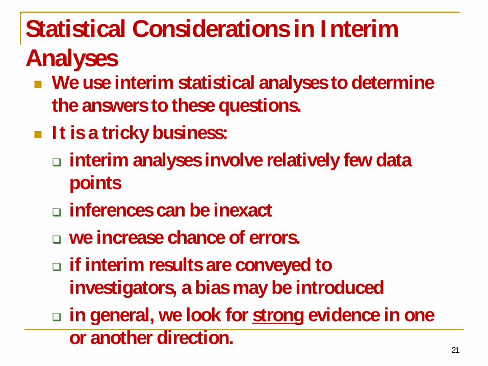
We use interim statistical analyses to determine the answers to these questions.It is a tricky business:

interim analyses involve relatively few data pointsinferences can be inexactwe increase chance of errors.if interim results are conveyed to investigators, a bias may be introducedin general, we look for strong evidence in one or another direction.

Statistical Considerations in Interim Analyses

22

Example: ECMO trialExtra-corporeal membrane oxygenation (ECMO) versus standard treatment for newborn infants with persistent pulmonary hypertension.N = 39 infants enrolled in studyTrial terminated after interim analysis

4/10 deaths in standard therapy arm0/9 deaths in ECMO armp = 0.054 (one-sided)

Questions:Is this result sufficient evidence on which to change routine practice?Is the evidence in favor of ECMO very strong?

23

Example: ISIS trialThe Second International Study of Infarct Survival (ISIS-2) Five week study of streptokinase versus placebo based on 17,187 patients with myocardial infarction. Trial continued until

12% death rate in placebo group9.2% death rate in streptokinase groupp < 0.000001

Issues:strong evidence in favor of streptokinase was available early onimpact would be greater with better precision on death rate, which would not be possible if trial stopped earlyearlier trials of streptokinase has similar results, yet little impact.

24

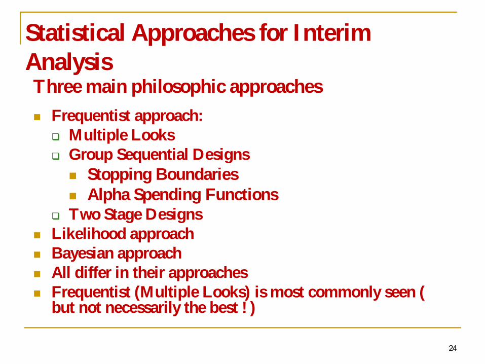
Statistical Approaches for Interim AnalysisThree main philosophic approaches

Frequentist approach:Multiple LooksGroup Sequential Designs

Stopping BoundariesAlpha Spending Functions

Two Stage DesignsLikelihood approachBayesian approachAll differ in their approachesFrequentist (Multiple Looks) is most commonly seen ( but not necessarily the best ! )

25

RCT (Randomized Clinical Trial with Trt A vs Trt B): Required Sample Size: 200

TRT A100

TRT B100

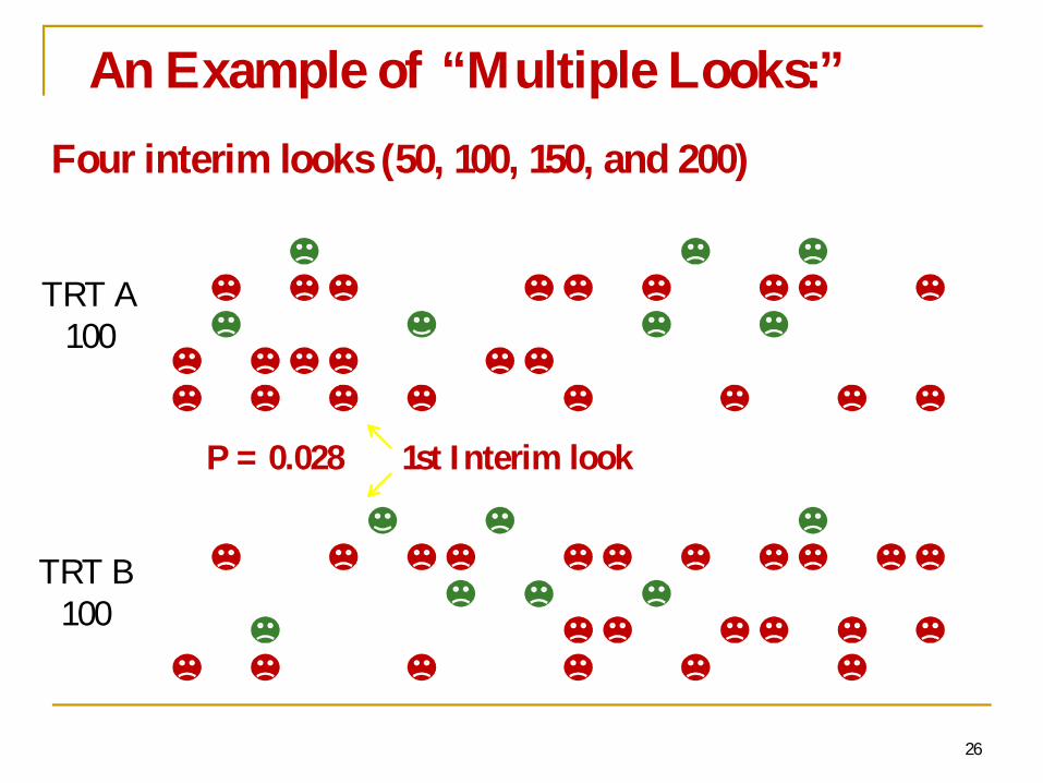
An Example of “Multiple Looks:”

26

Four interim looks (50, 100, 150, and 200)

TRT A100

TRT B100

1st Interim lookP = 0.028

An Example of “Multiple Looks:”

27

Four interim looks (50, 100, 150, and 200)

TRT A100

TRT B100

2nd Interim lookP = 0.38

An Example of “Multiple Looks:”

28

Four interim looks (50, 100, 150, and 200)

TRT A100

TRT B100

P = 0.028 P = 0.38 P = 0.62 P = 1.00

An Example of “Multiple Looks:”

P = 0.028

29

An Example of “Multiple Looks:”Consider planning a comparative trial in which two treatments are being compared for efficacy (response rate).

H0: p2 = p1

H1: p2 > p1

A standard design says that for 80% power and with alpha of 0.05, you need about 100 patients per arm based on the assumption p2 = 0.50, p1= 0.30 which results in 0.20 for the difference. So what happens if we find p < 0.05 before all patients are enrolled ?Why can’t we look at the data a few times in the middle of the trial and conclude that one treatment is better if we see p < 0.05?

30

The plots to the right show simulated data where p1= 0.40 and p2 = 0.50

In our trial, looking to find a difference between 0.30 to 0.50, we would not expect to conclude that there is evidence for a difference.

However, if we look after every 4 patients, we get the scenario where we would stop at 96 patients and conclude that there is a significant difference.

Number of Patients

Ris

k R

atio

0 50 100 150 200

0.0

0.5

1.0

1.5

Number of Patients

pval

ue

0 50 100 150 200

0.2

0.4

0.6

0.8

1.0

H1

31

If we look after every 10 patients, we get the scenario where we would not stop until all 200 patients were observed and would conclude that there is not a significant difference (p =0.40)

Number of Patients

Ris

k R

atio

50 100 150 200

1.0

1.2

1.4

1.6

Number of Patients

pval

ue

50 100 150 200

0.2

0.4

0.6

0.8

1.0

H 1

32

If we look after every 40 patients, we get the scenario where we would not stop either.

If we wait until the END of the trial (N = 200), then we estimate p1 to be 0.45 and p2 to be 0.52. The p-value for testing that there is a significant difference is 0.40.

Number of Patients

Ris

k R

atio

50 100 150 200

1.0

1.2

1.4

Number of Patients

pval

ue

50 100 150 200

0.2

0.4

0.6

0.8

1.0

H1

33

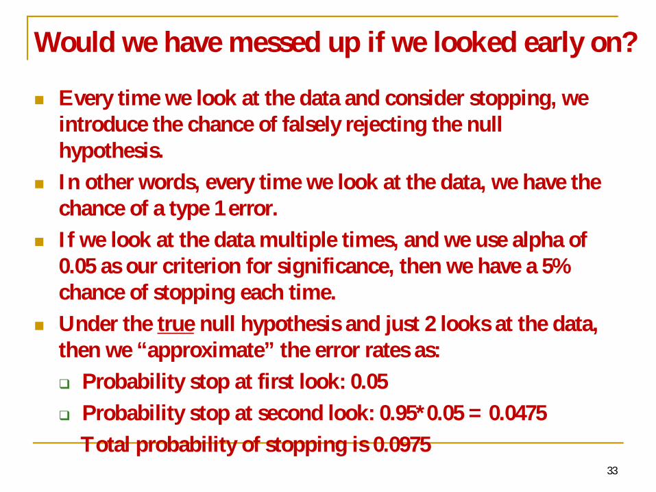
Would we have messed up if we looked early on?

Every time we look at the data and consider stopping, we introduce the chance of falsely rejecting the null hypothesis.In other words, every time we look at the data, we have the chance of a type 1 error.If we look at the data multiple times, and we use alpha of 0.05 as our criterion for significance, then we have a 5% chance of stopping each time.Under the true null hypothesis and just 2 looks at the data, then we “approximate” the error rates as:

Probability stop at first look: 0.05Probability stop at second look: 0.95*0.05 = 0.0475Total probability of stopping is 0.0975

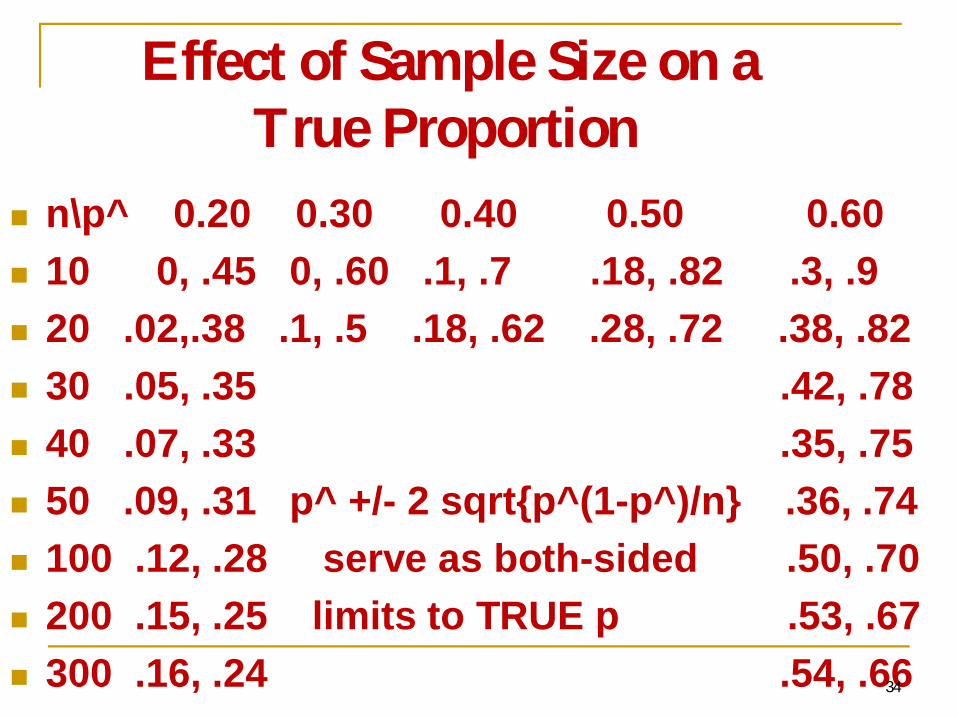
Effect of Sample Size on a True Proportion

n\p^ 0.20 0.30 0.40 0.50 0.60 10 0, .45 0, .60 .1, .7 .18, .82 .3, .920 .02,.38 .1, .5 .18, .62 .28, .72 .38, .8230 .05, .35 .42, .7840 .07, .33 .35, .7550 .09, .31 p^ +/- 2 sqrt{p^(1-p^)/n} .36, .74100 .12, .28 serve as both-sided .50, .70200 .15, .25 limits to TRUE p .53, .67300 .16, .24 .54, .6634

Effect of Sample Size on a True Proportion

n\p^ 0.2 0.3 0.4 0.5 0.6 400 0.16, 0.24500 0.17, 0.231000 .175, .225 1500 .18, .222000 .182, .218 p^ +/- 2 sqrt{p^(1-p^)/n}3000 .185, .215 serve as both-sided limits4000 .19, .21 for TRUE p5000 .19, .21

35

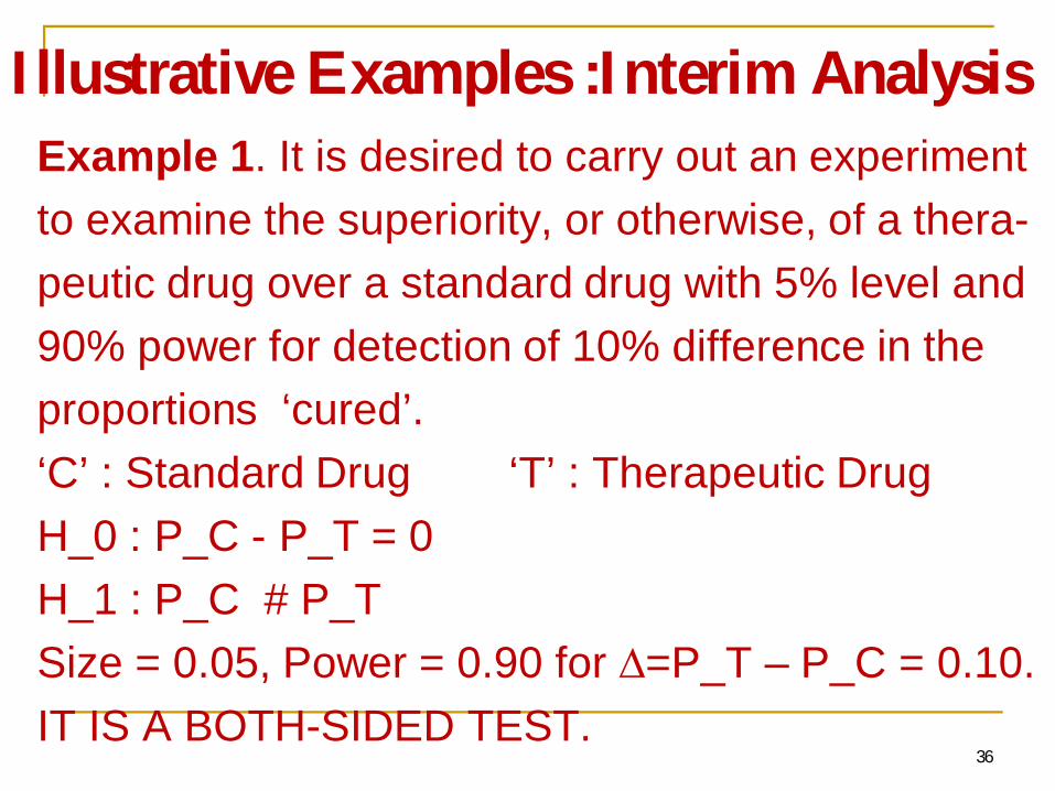
Illustrative Examples :Interim AnalysisExample 1. It is desired to carry out an experimentto examine the superiority, or otherwise, of a thera-peutic drug over a standard drug with 5% level and90% power for detection of 10% difference in the proportions ‘cured’. ‘C’ : Standard Drug ‘T’ : Therapeutic DrugH_0 : P_C - P_T = 0H_1 : P_C # P_TSize = 0.05, Power = 0.90 for =P_T – P_C = 0.10.IT IS A BOTH-SIDED TEST.

36

Determination of Sample Size for Full Analysis

37

Two-sided Test = 0.05; Z_ /2 = 1.96

Power = 0.90; = 0.10, Z_ = 1.282, =0.10N = 2(Z_ /2 + Z_ )^2 pbar(1-pbar)/ ^2

Assume pbar = 0.35 [suggestive cure rate] N = 2(1.96 + 1.282)^2 (0.35)(0.65)/(0.10)^2

= 21.021128 x 22.75= 478.23……480Conclusion: Each arm involves 480 subjects.

Full Experiment vs. Interim AnalysisFor Full Experiment : Needed 480 subjects in each ‘arm’.At the end of the entire experiment, suppose we observe :‘C’ : # cured = 156 out of 480 i.e., 32.5%‘T’ : # cured = 190 out of 480 i.e., 39.6%Therefore, p^_C = 0.325 and p^_T = 0.396.Hence, pbar = [p^_C + p^_T]/2 = 0.3605.Finally, we compute the value of z given by

38

Full Analysis…..Z_obs. = [p^_C – p^_T]/sqrt[pbar(1-pbar)2/N]

=[.325-.396]/sqrt[.36x.64x2/480] = -[.071]/sqrt[0.00192] = -2.29

In absolute value, z_obs. is computed as 2.29 which is more than the ‘critical’ value of z given by 1.96 [for a both-sided test with size 5%]. Hence, we conclude that the Null Hypothesis is ‘not tenable’, given the experimental outputs.

39

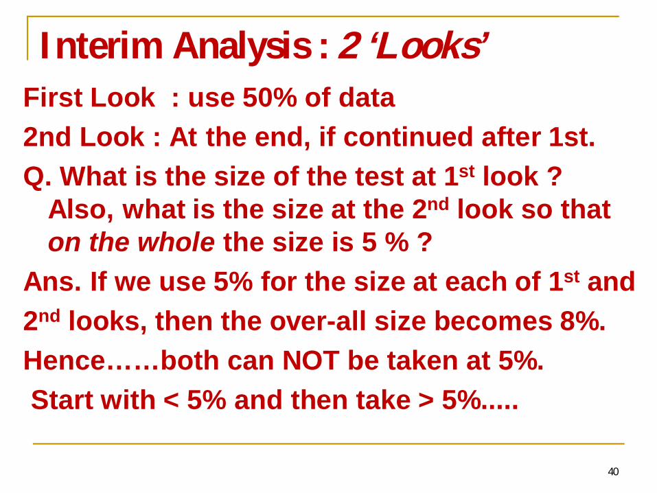
Interim Analysis : 2 ‘Looks’First Look : use 50% of data2nd Look : At the end, if continued after 1st.Q. What is the size of the test at 1st look ?

Also, what is the size at the 2nd look so that on the whole the size is 5 % ?

Ans. If we use 5% for the size at each of 1st and 2nd looks, then the over-all size becomes 8%.Hence……both can NOT be taken at 5%. Start with < 5% and then take > 5%.....

40

Interim Analysis : 2 Looks Defining Equation :

= P[ Z_I > z*] + P[ Z_I < z*, Z_{I,II} > z**] where Z_I and Z_II are based on 50% data in two identical and independent segments so that their distributions are identical. Further, Z_{I,II} = [z_I + z_II]/sqrt(2) is based on combined evidence of I & II and hence Z_I and Z_{I,II} are dependent.Choices of z* and z** : intricate formulae.

41

Interim Analysis : 2 Looks Z-computation….z_I obs. is to be based on 50% data upto the 1st look for each of ‘C’ and ‘T’.Data : C (90/240) & T(120/240) & n = 240.p^_C = 90/240 = 0.375; p^_T = 120/240=0.50pbar = (0.375 + 0.50)/2 = 0.4375.z_I obs. = [p^_C – p^_T]/sqrt[pbar(1-pbar)2/n]

= - [ 0.125 ]/sqrt{.4375x.5625x2/240}= - (0.125)/sqrt{0.002050}= - 2.76 implies ???

42

Interim Analysis : 2 Looks

43

Suggested cut-off points :Adopted for 2 Looks z_c Hebittle-Peto Pocock O’Brien-Fleming

z* 3.0 2.46 3.5z** 2.0 2.46 2.0 z_I obs. in absolute value = 2.76Conclusion ? Reject H_0 ….suggested by Pocock’s RuleContinue …suggested by other two. Finally, z = - 2.29 suggests acceptance of H_0 only by Pocock’s rule

Interim Analysis : 4 Looks Cut-off points : Suggested Rulesz_c Hebittle-Peto Pocock O’Brien-Fleming

z* 3.0 2.42 4.00z** 3.0 2.42 2.83

z*** 3.0 2.42 2.32z**** 2.0 2.42 2.00

• : 1st look; ** : 2nd look; *** : 3rd look and • **** : last [4th] look

44

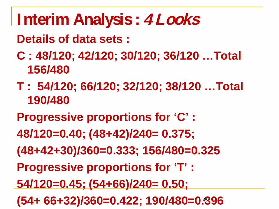
Interim Analysis : 4 Looks Details of data sets :C : 48/120; 42/120; 30/120; 36/120 …Total

156/480T : 54/120; 66/120; 32/120; 38/120 …Total

190/480Progressive proportions for ‘C’ :48/120=0.40; (48+42)/240= 0.375;(48+42+30)/360=0.333; 156/480=0.325 Progressive proportions for ‘T’ :54/120=0.45; (54+66)/240= 0.50;(54+ 66+32)/360=0.422; 190/480=0.39645

Interim Analysis : 4 Looks

Progressive computations of pbar……1st Look : pbar = (0.40 + 0.45)/2 = 0.4252nd Look : pbar = (0.375 + 0.50)/2 = 0.43753rd Look : pbar = ( 0.333 + 0.422)/2 = 0.36394th Look : pbar = (0.325 + 0.396)/2 = 0.3605

46

Interim Analysis : 4 Looks

Progressive Computations of z-statistic Generic Formula : z-obs. for ‘Look # i’ is the ratio of (a) [p^_C(i)– p^_T(i)] for i-th Look (b) sqrt[pbar(i)(1-pbar(i))2/n(i)]where pbar(i) corresponds to Look # i and also ‘n(i) ’ corresponds to size of each armof Look # i for each i = 1, 2, 3,4.

Note : n(1)=120; n(2)=240; n(3)=360, n(4)=480 47

Interim Analysis : 1st Look z_(Look I) obs.

= [p^_C – p^_T]/sqrt[pbar(1-pbar)2/n*]= [ 0.40-0.45 ]/sqrt{.425x.575x2/120}

= - (0.05)/sqrt{0.004073}= -0.7835

Conclusion : All Rules are suggestive of Continuation to 2nd Look

48

Interim Analysis : 2nd Look

z_(Look II) obs. = [p^_C – p^_T]/sqrt[pbar(1-pbar)2/n**]= [0.375-0.50 ]/sqrt{.4375x.5625x2/240}= - (0.125)/sqrt{0.002050}= - 2.76

Conclusion : Reject H_0 by Pocock’s RuleHowever, continue to 3rd Look according to the other two rules.

49

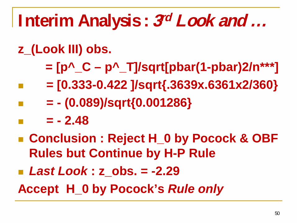
Interim Analysis : 3rd Look and …z_(Look III) obs.

= [p^_C – p^_T]/sqrt[pbar(1-pbar)2/n***]= [0.333-0.422 ]/sqrt{.3639x.6361x2/360}= - (0.089)/sqrt{0.001286}= - 2.48

Conclusion : Reject H_0 by Pocock & OBF Rules but Continue by H-P RuleLast Look : z_obs. = -2.29

Accept H_0 by Pocock’s Rule only

50

Data Analysis….InterpretationsRelative Merits of Decision Rules :Pocock’s Rule : Maintains uniformity in critical values ….so …apparently ‘conservative’ at the start…slowly turns into ‘liberal’ !Other Rules : Liberal at the start and conservative at the end…..All Rules have to maintain the ‘averaging principle’ to meet alpha at the end.No Rule can be strict/liberal all through the Looks.

51

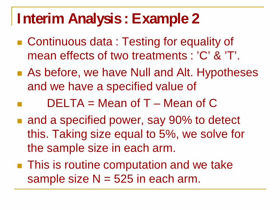
Interim Analysis : Example 2Continuous data : Testing for equality of mean effects of two treatments : ’C’ & ’T’. As before, we have Null and Alt. Hypotheses and we have a specified value of

DELTA = Mean of T – Mean of C and a specified power, say 90% to detect this. Taking size equal to 5%, we solve for the sample size in each arm.This is routine computation and we take sample size N = 525 in each arm.

Full Analysis : Sample Size ComputationAssume normal distribution with sigma = 5.Two-sided Test

= 0.05; Z_ /2 = 1.96Power = 0.90; = 0.10, Z_ = 1.282,

= 0.20 times sigma = 20% of sigma = 1.0N = 2(Z_ /2 + Z_ )^2 x sigma^2 / ^2

= 2(1.96 + 1.282)^2 / 0.04 = 525 [approx.]

We can think of 5 Looks altogether…at equalSteps…..each with approx. 105 observations.

Interim Analysis…Example contd.

Details of data sets : (mean, sample size)C : (30.5,105); (31.8, 105); (29.7, 105);

(30.2, 105); (31.3, 105) T : (31.7,105); (32.0, 105); (30.8, 105);

(33.7, 105); (32.8, 105) Progressive sample means for ‘C’ :30.5, 31.15, 30.67, 30.55, 30.70Progressive sample means for ‘T’ :31.7, 31.85, 30.83, 32.55, 32.60

Interim Analysis : Example contd….Progressive Computations of z-statistic Generic Formula : z-obs. for ‘Look # i’ is the ratio of (a) [mean_C(i)– mean_T(i)] for i-th Look (b) sigma times Sqrt 2/n(i)]where mean refers to sample mean for and also ‘n(i) ’ corresponds to size of each armof Look # i for each i = 1, 2, 3,4, 5.

Note : n(1)=105; n(2)=210; n(3)=315, n(4)=420 and n(5) = 525.

Interim Analysis : Example contd. Cut-off points : Suggested Rulesz_c Hebittle-Peto Pocock O’Brien-Fleming

z* 3.0 2.60 4.56z** 3.0 2.60 3.23

z*** 3.0 2.60 2.63z**** 3.0 2.60 2.28z***** 2.0 2.60 2.00

• : 1st look; ** : 2nd look; *** : 3rd look; • **** : 4th look & ***** : Last [5th] look

Interim Analysis…Example contd.

z_(Look I) obs. = [mean_C – mean_T]/sigma x sqrt[2/n*]

= - [ 1.2] / 5 x sqrt{2/105}= - 1.74

Conclusion : Continue to 2nd Look

Interim Analysis : Example contd.z_(Look II) obs.

= [mean_C – mean_T]/sigma x sqrt[2/n**]= - [ 0.7 ] / 5 x sqrt{2/210}

= - 1.43

Conclusion : Continue to 3rd Look

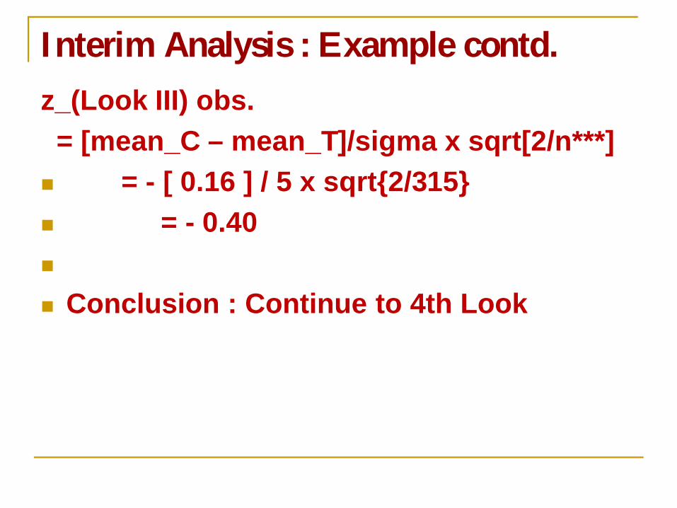
Interim Analysis : Example contd.z_(Look III) obs.

= [mean_C – mean_T]/sigma x sqrt[2/n***]= - [ 0.16 ] / 5 x sqrt{2/315}

= - 0.40

Conclusion : Continue to 4th Look

Interim Analysis : Example contd.z_(Look IV) obs. = [mean_C – mean_T]/sigma x sqrt[2/n****]

= - [ 2.0 ] / 5 x sqrt{2/420}= - 5.80

Conclusion : Stop and Reject H_0. Strong evidence against H_0 and yet 105 observations per arm are left to be studied. What if the expt was continued till the end anyway ?

Interim Analysis : Example contd.z_(Look V) obs.

= [mean_C – mean_T]/sigma x sqrt[2/n*****]= - [ 1.90 ] / 5 x sqrt{2/525}

= - 6.16

Conclusion : Reject H_0. Quite a strong evidence against H_0