Intercept of Frequency Agility Signal using Coding Nyquist Folding ...
10
Intercept of Frequency Agility Signal using Coding Nyquist Folding Receiver KEYU LONG School of Electronic Engineering University of Electronic Science and Technology of China No. 2006, Xiyuan Avenue, West Hi-Tech Zone, Chengdu CHINA [email protected] Abstract: - The parameter estimation of the frequency agility (FA) signal using the coding Nyquist folding receiver (CNYFR) is presented. The estimation algorithm adopting linear frequency modulation (LFM) as the local analogue modulation is derived. The Nyquist zone is estimated by the pseudo Wigner-Ville distribution (PWVD) and the hopping frequencies are calculated by the maximum likelihood (ML) method. Simulations show that CNYFR with analogue modulation of LFM has better performance than the sinusoidal frequency modulation (SFM) one, and the parameter estimation accuracy is acceptable when the SNR is above 0dB. Key-Words: - Frequency agility signal; Nyquist folding receiver; coding; linear frequency modulation (LFM). 1 Introduction The frequency agility (FA) signal, also known as the frequency hopping (FH) signal, has been widely applied in radar, communication, sonar and other fields because of its good performance in low possibility of intercept and anti-interference. In the field of radar, FA has always been a research focus. Bellegarda studied multiple access FH signals using a synthesis tool of the hit array in the context of coherent active radar [1]. Morrison proposed an approach which allows the frequency spectrum to be greatly under-sampled to provide a greater effective bandwidth for a stepped frequency continuous wave (SF-CW) synthetic aperture radar (SAR) [2]. Becker studied passive localization of FA radars for angle and frequency measurements [3]. Rogers presented analytical techniques for evaluating the performance of FH radars based on the autocorrelation properties of the frequency selection process [4]. Lellouch investigated an agile orthogonal frequency division multiple (OFDM) waveform to solve the problem of Doppler frequency shift in FA [5]. The bandwidth of a FA radar signal could be greater than 10GHz. For the intercept receiver of the FA signal, the main question is how to intercept such a wide bandwidth under the condition of low sampling rate less than 3Giga sample per second (GSPS). Fortunately, the FA signal could be regarded as a kind of sparse signals, and could be processed by the recent powerful concept denoted as compressed sensing (CS). Under CS, we may intercept the radar signals with low sampling rate. The concept of CS was proposed by Candes and Donoho [6-7], et al in 2006. From then on, many scholars studied the application of CS in various aspects. Herman studied a high-resolution radar via CS [8]. Ma used CS for surface characterization and metrology [9]. Potter applied CS in radar imaging [10]. Provost studied the application of CS for photo- acoustic tomography [11]. Flandrin discussed the connection between CS and time frequency distribution, and showed that improved representations can be obtained with the cost of computational complexity [12]. Now CS has been applied to a variety fields such as receiver and camera. In the receiver side, some scholars have proposed different structures. Tropp and Laska developed an architecture called the random demodulator, which consists of a pseudorandom number generator, a mixer, an accumulator (or a low pass filter) and a low rate analog-to-digital converter (ADC). First, they mixed the input signal with a high-rate pseudo noise sequence. Then, the output signal passes through a filter with a narrow passband and a few samples with a relatively low rate compared to the Nyquist rate are acquired. The system can be used to perform the spectrum sensing, geophysical imaging as well as radar and sonar imaging. The major advantage of the random demodulator is that it avoids a high-rate ADC, and expands the CS theory to analog signals. Also, it is robust against noise. However, some engineering issues should be considered such as the speed of the mixer and the WSEAS TRANSACTIONS on SIGNAL PROCESSING Keyu Long ISSN: 1790-5052 82 Issue 2, Volume 7, April 2011
Transcript of Intercept of Frequency Agility Signal using Coding Nyquist Folding ...
Intercept of Frequency Agility Signal using Coding Nyquist Folding
Receiver
KEYU LONG
School of Electronic Engineering
University of Electronic Science and Technology of China
No. 2006, Xiyuan Avenue, West Hi-Tech Zone, Chengdu
CHINA
Abstract: - The parameter estimation of the frequency agility (FA) signal using the coding Nyquist folding
receiver (CNYFR) is presented. The estimation algorithm adopting linear frequency modulation (LFM) as the
local analogue modulation is derived. The Nyquist zone is estimated by the pseudo Wigner-Ville distribution
(PWVD) and the hopping frequencies are calculated by the maximum likelihood (ML) method. Simulations
show that CNYFR with analogue modulation of LFM has better performance than the sinusoidal frequency
modulation (SFM) one, and the parameter estimation accuracy is acceptable when the SNR is above 0dB.
Key-Words: - Frequency agility signal; Nyquist folding receiver; coding; linear frequency modulation (LFM).
1 Introduction The frequency agility (FA) signal, also known as the
frequency hopping (FH) signal, has been widely
applied in radar, communication, sonar and other
fields because of its good performance in low
possibility of intercept and anti-interference. In the
field of radar, FA has always been a research focus.
Bellegarda studied multiple access FH signals using
a synthesis tool of the hit array in the context of
coherent active radar [1]. Morrison proposed an
approach which allows the frequency spectrum to be
greatly under-sampled to provide a greater effective
bandwidth for a stepped frequency continuous wave
(SF-CW) synthetic aperture radar (SAR) [2]. Becker
studied passive localization of FA radars for angle
and frequency measurements [3]. Rogers presented
analytical techniques for evaluating the performance
of FH radars based on the autocorrelation properties
of the frequency selection process [4]. Lellouch
investigated an agile orthogonal frequency division
multiple (OFDM) waveform to solve the problem of
Doppler frequency shift in FA [5].
The bandwidth of a FA radar signal could be
greater than 10GHz. For the intercept receiver of the
FA signal, the main question is how to intercept such
a wide bandwidth under the condition of low
sampling rate less than 3Giga sample per second
(GSPS). Fortunately, the FA signal could be
regarded as a kind of sparse signals, and could be
processed by the recent powerful concept denoted as
compressed sensing (CS). Under CS, we may
intercept the radar signals with low sampling rate.
The concept of CS was proposed by Candes and
Donoho [6-7], et al in 2006. From then on, many
scholars studied the application of CS in various
aspects. Herman studied a high-resolution radar via
CS [8]. Ma used CS for surface characterization and
metrology [9]. Potter applied CS in radar imaging
[10]. Provost studied the application of CS for photo-
acoustic tomography [11]. Flandrin discussed the
connection between CS and time frequency
distribution, and showed that improved
representations can be obtained with the cost of
computational complexity [12]. Now CS has been
applied to a variety fields such as receiver and
camera.
In the receiver side, some scholars have proposed
different structures. Tropp and Laska developed an
architecture called the random demodulator, which
consists of a pseudorandom number generator, a
mixer, an accumulator (or a low pass filter) and a
low rate analog-to-digital converter (ADC). First,
they mixed the input signal with a high-rate pseudo
noise sequence. Then, the output signal passes
through a filter with a narrow passband and a few
samples with a relatively low rate compared to the
Nyquist rate are acquired. The system can be used to
perform the spectrum sensing, geophysical imaging
as well as radar and sonar imaging. The major
advantage of the random demodulator is that it
avoids a high-rate ADC, and expands the CS theory
to analog signals. Also, it is robust against noise.
However, some engineering issues should be
considered such as the speed of the mixer and the
WSEAS TRANSACTIONS on SIGNAL PROCESSING Keyu Long
ISSN: 1790-5052 82 Issue 2, Volume 7, April 2011
impulse response of the filter [13-14]. Romberg
proposed another structure called random
convolution. It circularly convolves the input signal
with a random pulse and then subsamples the output
signal. Since the system is universal and allows fast
computations, it is perfect to be a theoretical sensing
strategy. Some applications include radar imaging
and Fourier optics. The random convolution system
is simpler and more efficient than other random
acquisition techniques. Further, the system is suited
to a wide range of compressed signals. However, the
realization of random pulse is a challenging problem.
For instance, whether different shifts of the pulse are
orthogonal is still a problem [15-16].
In the application of camera, Takhar developed a
new camera architecture called compressive imaging
camera, which uses a digital micro mirror array to
acquire linear projections of an image onto
pseudorandom binary patterns. The most exciting
feature of the system is that it can be adapted to
image at wavelengths with conventional charge-
coupled device (CCD) and complementary metal
oxide semiconductor (CMOS) imagers, and it has
good features including simplicity, universality,
robustness, and scalability. However, some problems
still exist as follows; for example, more other
measurement bases can be implemented, and higher-
quality reconstruction of images needs further studies.
Besides, a more complex photon sensing element can
be used to colour, multispectral, and hyper spectral
imaging [17].
Driven by the idea of CS, Fudge proposed the
Nyquist Folding Receiver (NYFR) [18]. This type of
receiver overcomes the disadvantages of the
traditional sub-sampling technique, only aiming at a
particular Nyquist sampling, and avoids frequency
sweep. The key of the NYFR is that the Nyquist zone
could be mapped to a parameter of the local analogue
modulated signal on the received signals, and then
we can sample the received signals which contain the
additional Nyquist zone information by a low
sampling rate. By changing the bandwidth of local
analogue modulation and the channel number, we
can achieve the whole probability interception of a
wideband or ultra-wideband signal in one channel
without using frequency sweep. However, the
structure of NYFR is easily affected by noise at the
zero crossing rising (ZCR) time when controlling the
radio frequency (RF) sample clock of shape pulse
using a full analogue structure for wideband
modulation. Besides, the structure of single channel
limits interception bandwidth mostly and the
implementation of sinusoidal frequency modulation
(SFM) as a local analogue modulation is difficult.
This paper presents an improved structure marked
as coding NYFR (CNYFR), also called dual channel
NYFR (DCNYFR) to realize the interception of the
FA signal, and shows the algorithm using pseudo
Wigner-Ville distribution (PWVD) for the estimation
of the Nyquist zone. Moreover, since linear
frequency modulation (LFM) is easier to be
generated, we adopt LFM as the local analogue
modulation instead of SFM.
The rest of the paper is organized as follows.
Section 2 analyses the structure for CNYFR in
details, and gives the advantages of dual-channel.
Section 3 describes the estimation of Nyquist zone.
Section 4 provides simulations. Finally, section 5
concludes the paper.
2 Coding Nyquist Folding Receiver With continued improvements in digital signal
processing (DSP) technology, the ADC is becoming
one of the bottlenecks in a variety of signal
applications ranging from radar to communications,
where the information is processed within extremely
wide RF bandwidths. Since the environment of
signal applications is generally sparse, it is feasible
to reduce the sample rate. Fudge considered the
information sampling of these sparse signals and
presented a practical receiving structure called
NYFR which can be applied to the direct processing
of high RF signals.
2.1 Structure for CNYFR We pay attention to the NYFR which is an analog-to-
information receiver architecture. The key technique
is that it folds the multiple original signal component
frequencies into a narrow bandwidth prior to ADC.
In this case, the sample rate of ADC can be reduced
obviously. Base on the architecture of the NYFR, we
can make some advances and propose this CNYFR.
The structure of the CNYFR is shown in Fig.1.
Assume that the input signal is FA, and the agile
range is from several hundreds of MHz to 20GHz.
Besides, we assume the input analog signal has been
pre-processed into a complex signal. Firstly, the
input signal is filtered by a ultra wideband (UWB)
low-pass filter (LPF1) whose passband is up to
20GHz to remove the out-of-band noise to get the
complex signal ( )x t . Then, ( )x t is multiplied by
( )ip t , 1,2i = , to obtain the modulated signal
( ) ( ) ( )i ir t x t p t= , then ( )ir t is filtered by the second
complex low-pass filter (LPF2) with the passband
[ ]/ 2 / 2s sf f− to get the signal ( )is t , where sf is
WSEAS TRANSACTIONS on SIGNAL PROCESSING Keyu Long
ISSN: 1790-5052 83 Issue 2, Volume 7, April 2011
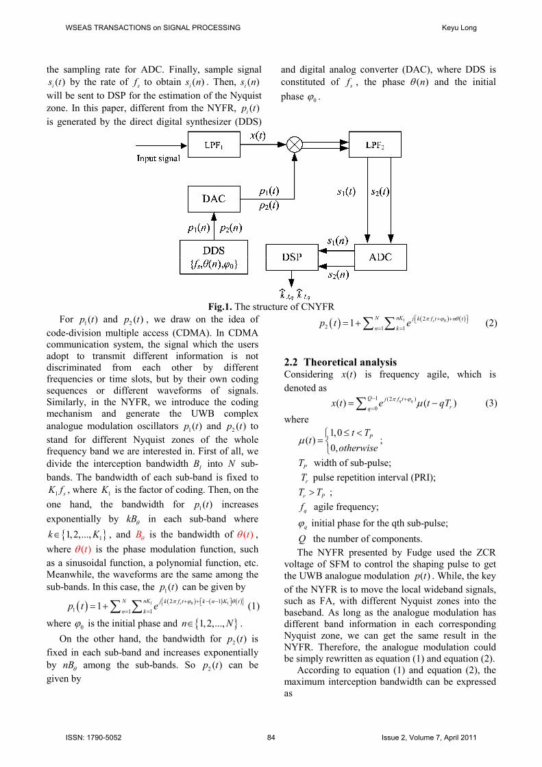
the sampling rate for ADC. Finally, sample signal
( )is t by the rate of sf to obtain ( )is n . Then, ( )is n
will be sent to DSP for the estimation of the Nyquist
zone. In this paper, different from the NYFR, ( )ip t
is generated by the direct digital synthesizer (DDS)
and digital analog converter (DAC), where DDS is
constituted of sf , the phase ( )nθ and the initial
phase 0ϕ .
Fig.1. The structure of CNYFR
For 1( )p t and 2 ( )p t , we draw on the idea of
code-division multiple access (CDMA). In CDMA
communication system, the signal which the users
adopt to transmit different information is not
discriminated from each other by different
frequencies or time slots, but by their own coding
sequences or different waveforms of signals.
Similarly, in the NYFR, we introduce the coding
mechanism and generate the UWB complex
analogue modulation oscillators 1( )p t and 2 ( )p t to
stand for different Nyquist zones of the whole
frequency band we are interested in. First of all, we
divide the interception bandwidth IB into N sub-
bands. The bandwidth of each sub-band is fixed to
1 sK f , where 1K is the factor of coding. Then, on the
one hand, the bandwidth for 1( )p t increases
exponentially by kBθ in each sub-band where
{ }11,2,...,k K∈ , and Bθ is the bandwidth of ( )tθ ,
where ( )tθ is the phase modulation function, such
as a sinusoidal function, a polynomial function, etc.
Meanwhile, the waveforms are the same among the
sub-bands. In this case, the 1( )p t can be given by
( ) ( ) ( ) ( ){ }1 0 12 1
1 1 11
sN nK j k f t k n K t
n kp t e
π ϕ θ+ + − − = =
= +∑ ∑ (1)
where 0ϕ is the initial phase and { }1,2,...,n N∈ .
On the other hand, the bandwidth for 2 ( )p t is
fixed in each sub-band and increases exponentially
by nBθ among the sub-bands. So 2 ( )p t can be
given by
( ) ( ) ( )1 02
2 1 11 s
N nK j k f t n t
n kp t e
π ϕ θ + + = =
= +∑ ∑ (2)
2.2 Theoretical analysis Considering ( )x t is frequency agile, which is
denoted as
1 (2 )
0( ) ( )q q
Q j f t
rqx t e t qT
π ϕ µ− +
== −∑ (3)
where
1,0( )
0,
Pt Tt
otherwiseµ
≤ <=
;
PT width of sub-pulse;
rT pulse repetition interval (PRI);
r PT T> ;
qf agile frequency;
qϕ initial phase for the qth sub-pulse;
Q the number of components.
The NYFR presented by Fudge used the ZCR
voltage of SFM to control the shaping pulse to get
the UWB analogue modulation ( )p t . While, the key
of the NYFR is to move the local wideband signals,
such as FA, with different Nyquist zones into the
baseband. As long as the analogue modulation has
different band information in each corresponding
Nyquist zone, we can get the same result in the
NYFR. Therefore, the analogue modulation could
be simply rewritten as equation (1) and equation (2).
According to equation (1) and equation (2), the
maximum interception bandwidth can be expressed
as
WSEAS TRANSACTIONS on SIGNAL PROCESSING Keyu Long
ISSN: 1790-5052 84 Issue 2, Volume 7, April 2011
1( 1 / 2)I sB NK f= + (4)
After being mixed and filtered by LPF2, the
outputs should be
( )( ) ( )
( )
, , 0 ,
1
21
0
q s H q q H q I qj f f k t k k tQ
q
r
s t
e
t qT
π ϕ ϕ θ
µ
− + − −− =
=
⋅
−
∑ (5)
( )( ) ( )
( )
, , 0 ,
2
21
0
q s H q q H q J qj f f k t k k tQ
q
r
s t
e
t qT
π ϕ ϕ θ
µ
− + − −− =
=
⋅
−
∑ (6)
where
( ), , 1 /I q q J q s sk round f k K f f = − ;
, 1/J q q sk f K f = ;
⋅ stands for round down;
[ ], 0 1J qk N∈ − ;
[ ], 11I qk K∈ .
, , , 1( 1)I q H q H qk k n K= − − (7)
, , 1J q H qk n= − (8)
Substituting equation (8) into equation (7), we
get
, , , 1H q I q J qk k k K= + (9)
Sample 1( )s t and 2 ( )s t then
( )( ) ( )
( )
, , 0 ,
1
21
0
q s H q s q H q I q sj f f k nT k k nTQ
q
s r
s n
e
nT qT
π ϕ ϕ θ
µ
− + − −− =
=
⋅
−
∑ (10)
( )( ) ( )
( )
, , 0 ,
2
21
0
q s H q s q H q J q sj f f k nT k k nTQ
q
s r
s n
e
nT qT
π ϕ ϕ θ
µ
− + − −− =
=
⋅
−
∑ (11)
where 1/s sT f= is the sampling interval.
From equation (10), we know that the qth sub-
pulse of the output ( )1s n is a wideband signal
whose center frequency, bandwidth and initial phase
are ,q s H qf f k− , 1 ,s I qB k Bθ= and , 0q H qkϕ ϕ− ,
respectively. The qth sub-pulse of the output ( )2s n
is also a wideband signal which has the same centre
frequency and initial phase but different bandwidth
2 ,s J qB k Bθ= .
2.3 The choice of the local analogue
modulation In this paper, we chose frequency modulation (FM)
as the local analogue modulation. Like the
amplitude modulation (AM), FM is well known as a
broadcast signal format for communication. In
particular, the LFM signal is a kind of FM signal
whose instantaneous frequency (IF) is modulated by
a linear signal. Because of low probability of
intercept, it is one of the most important signals in
radar field, which has high range resolution, inhibits
leakage and near field interference. Due to its good
pulse compression characteristic, many high
resolution radars such as SARs use this kind of FM
waveform. It is a mature technology to generate the
waveform; therefore, we are more inclined to
choose LFM than SFM as the local analogue
modulation.
2.4 The advantage of Dual-channel
The signals ( )1s t and ( )2s t are just in one Nyquist
zone namely the baseband [ / 2 / 2]s sf f− .
According to the Nyquist sampling theorem, the
condition of sampling without aliasing is
( ), 1
/ 1 / 2 /
I q
I s
s
k B K B
B f B N
f
θ θ
θ
≤
= −
≤
(12)
Suppose that we use SFM function ( )tθ , i.e.,
( ) ( )sin 2e ft t f tθ π= (13)
The instantaneous frequency of equation (13) is
( )cos 2e f ff t f f tπ= , therefore 2 e fB t fθ = , where
/e ft f f= ∆ is the factor of frequency modulation,
f∆ the frequency drift and ff the frequency of the
modulation signal.
Equation (12) could be rewritten as
2
2
se
I f s f
f Nt
B f f f≤
− (14)
Generally, for SFM, et is one of the most
important parameters we need to design. Compared
with the single channel method, the dual-channel
can realize wider IB with the same parameters of
SFM. When s If B≪ and 2 / 2e s I ft f N B f≤ , IB can
be widened N times.
We can recover the signal without distortion
when equation (12) is satisfied. For electronic
reconnaissance, when the interception frequency
range is 21GHz, the sampling rate is 2GHz and
1 5K = , we get 2N = from equation (4), then
400Bθ ≤ MHz.
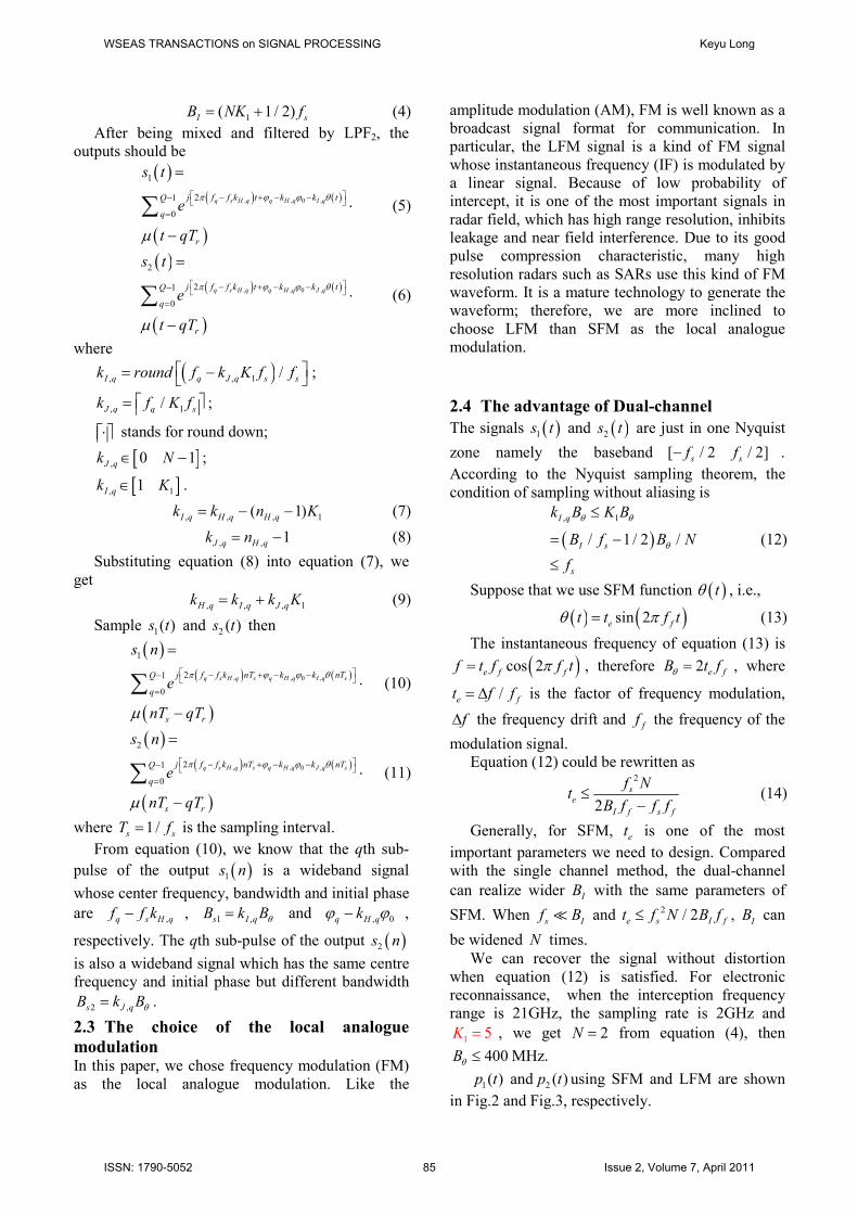
1( )p t and 2 ( )p t using SFM and LFM are shown
in Fig.2 and Fig.3, respectively.
WSEAS TRANSACTIONS on SIGNAL PROCESSING Keyu Long
ISSN: 1790-5052 85 Issue 2, Volume 7, April 2011
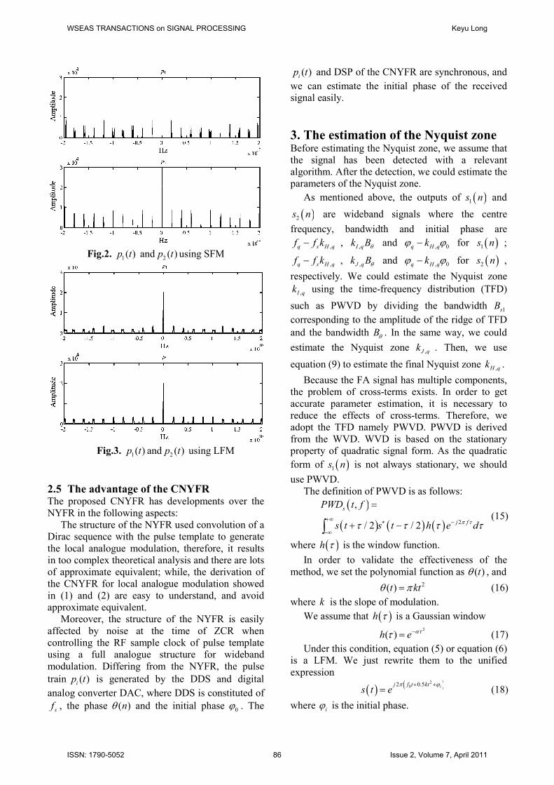
Fig.2. 1( )p t and 2 ( )p t using SFM
Fig.3. 1( )p t and 2 ( )p t using LFM
2.5 The advantage of the CNYFR The proposed CNYFR has developments over the
NYFR in the following aspects:
The structure of the NYFR used convolution of a
Dirac sequence with the pulse template to generate
the local analogue modulation, therefore, it results
in too complex theoretical analysis and there are lots
of approximate equivalent; while, the derivation of
the CNYFR for local analogue modulation showed
in (1) and (2) are easy to understand, and avoid
approximate equivalent.
Moreover, the structure of the NYFR is easily
affected by noise at the time of ZCR when
controlling the RF sample clock of pulse template
using a full analogue structure for wideband
modulation. Differing from the NYFR, the pulse
train ( )ip t is generated by the DDS and digital
analog converter DAC, where DDS is constituted of
sf , the phase ( )nθ and the initial phase 0ϕ . The
( )ip t and DSP of the CNYFR are synchronous, and
we can estimate the initial phase of the received
signal easily.
3. The estimation of the Nyquist zone Before estimating the Nyquist zone, we assume that
the signal has been detected with a relevant
algorithm. After the detection, we could estimate the
parameters of the Nyquist zone.
As mentioned above, the outputs of ( )1s n and
( )2s n are wideband signals where the centre
frequency, bandwidth and initial phase are
,q s H qf f k− , ,I qk Bθ and , 0q H qkϕ ϕ− for ( )1s n ;
,q s H qf f k− , ,J qk Bθ and , 0q H qkϕ ϕ− for ( )2s n ,
respectively. We could estimate the Nyquist zone
,I qk using the time-frequency distribution (TFD)
such as PWVD by dividing the bandwidth 1sB
corresponding to the amplitude of the ridge of TFD
and the bandwidth Bθ . In the same way, we could
estimate the Nyquist zone ,J qk . Then, we use
equation (9) to estimate the final Nyquist zone ,H qk .
Because the FA signal has multiple components,
the problem of cross-terms exists. In order to get
accurate parameter estimation, it is necessary to
reduce the effects of cross-terms. Therefore, we
adopt the TFD namely PWVD. PWVD is derived
from the WVD. WVD is based on the stationary
property of quadratic signal form. As the quadratic
form of ( )1s n is not always stationary, we should
use PWVD.
The definition of PWVD is as follows:
( )
( ) ( ) ( ) 2
,
/ 2 / 2
s
j f
PWD t f
s t s t h e dπ ττ τ τ τ+∞ ∗ −
−∞
=
+ −∫ (15)
where ( )h τ is the window function.
In order to validate the effectiveness of the
method, we set the polynomial function as ( )tθ , and
2( )t ktθ π= (16)
where k is the slope of modulation.
We assume that ( )h τ is a Gaussian window
2
( )h e αττ −= (17)
Under this condition, equation (5) or equation (6)
is a LFM. We just rewrite them to the unified
expression
( ) ( )202 0.5 ij f t kt
s t eπ ϕ+ +
= (18)
where iϕ is the initial phase.
WSEAS TRANSACTIONS on SIGNAL PROCESSING Keyu Long
ISSN: 1790-5052 86 Issue 2, Volume 7, April 2011
The product signal is
( ) ( )( ) ( )
( ) ( )
( )
20
20
0
2 /2 1/2 /2
2 /2 1/2 /2
2
/ 2 / 2
i
i
j f t k t
j f t k t
j f kt
s t s t
e
e
e
π τ τ ϕ
π τ τ ϕ
π τ
τ τ∗
+ + + +
− − + − +
+
+ −
= ⋅
=
(19)
Then inserting equation (19) into equation (15),
the PWVD of LFM is as follows:
( )
( ) ( ) ( )( ) ( )0
2
2 2
,
/ 2 / 2
s
j f
j f kt j f
PWD t f
s t s t h e d
e h e d
π τ
π τ π τ
τ τ τ τ
τ τ
+∞ ∗ −
−∞
+∞ + −
−∞
=
+ −
=
∫
∫
(20)
According to the convolution property of the
Fourier transform, we know that the product in time
domain means convolution in frequency domain.
Therefore, equation (20) is equal to
( ) ( ) ( )0,sPWD t f f f kt H fδ= − + ⊗ (21)
where the mark ⊗ denotes one dimension
convolution at frequency f . Here we use
( )
( )
( )
0
0
2 2
2
0
j f kt j f
j f kt f
e e d
e d
f f kt
π τ π τ
π τ
τ
τ
δ
+∞ + −
−∞
+∞ + −
−∞=
= − +
∫
∫ (22)
and
( )2 /1/2 1/2( )f
H f eπ απ α −−= (23)
is the Fourier transform of ( )h τ , which is
monotonously decreasing, and we can get the
maximum of ( )H f at 0f = .
Then by equation (21) and equation (23), we can
get
( ) ( )( )
( )( )20
0
/1/2 1/2
,s
f f kt
PWD t f H f f kt
eπ απ α − − +−
= − +
= (24)
The ridge of PWVD contains important
information about the characteristics of the signal.
We put forward an algorithm to extract the ridge.
The idea is to search for the maximum of
( ),sPWD t f along f . Thus, the ridge of
( ),sPWD t f is given by
( ){ }( ) argmax ,sf
r t PWD t f= (25)
Based on analysis above, we know that equation
(24) gets the maximum at 0f f kt= + , then
( ) 0( )r t f t f kt= = + (26)
Under this condition, we can get the bandwidth
from the amplitude of the ridge of PWVD. Further,
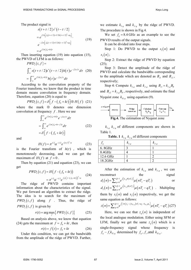
we estimate ,I qk and ,J qk by the ridge of PWVD.
The procedure is shown in Fig.4.
We set 8.4qf = GHz as an example to see the
PWVD results of the output signals.
It can be divided into four steps.
Step 1: Do PWVD to the output ( )1s n and
( )2s n ;
Step 2: Extract the ridge of PWVD by equation
(25);
Step 3: Detect the amplitude of the ridge of
PWVD and calculate the bandwidths corresponding
to the amplitude which are denoted as 1sB and 2sB ,
respectively;
Step 4: Compute ,I qk and ,J qk using 1 ,s I qB k Bθ=
and 2 ,s J qB k Bθ= , respectively, and estimate the final
Nyquist zone ,H qk using equation (9).
Fig.4. The estimation of Nyquist zone
,I qk ,J qk of different components are shown in
Table 1.
Table. 1 ,I qk ,J qk of different components
qf ,I qk ,J qk
6. 8GHz 3 1
8.4GHz 4 1
12.6 GHz 1 2
18.2GHz 4 2
After the estimation of ,I qk and ,J qk , we can
reconstruct the signal
( ) ( ) ( ),1
1 0
I q sQ j k nT
s rqd n e nT qT
θ µ −
== −∑ or
( ) ( ) ( ),1
2 0
J q sQ j k nT
s rqd n e nT qT
θ µ −
== −∑ . Multipling
them by ( )1s n and ( )2s n respectively, we get the
same equation as follows:
( ) ( ) ( ), , 021
0
q s H q s q H qj f f k nT kQ
s rqz n e nT qT
π ϕ ϕµ
− + −− =
= −∑ (27)
Here, we can see that ( )qz n is independent of
the local analogue modulation. Either using SFM or
LFM, finally we get the same ( )qz n which is a
single-frequency signal whose frequency is
,q s H qf f k− determined by qf , sf ,and ,H qk .
WSEAS TRANSACTIONS on SIGNAL PROCESSING Keyu Long
ISSN: 1790-5052 87 Issue 2, Volume 7, April 2011
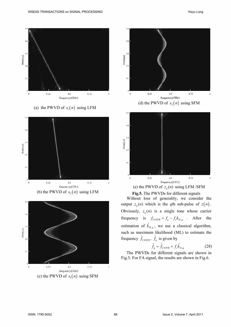
(a) the PWVD of ( )1s n using LFM
(b) the PWVD of ( )2s n using LFM
(c) the PWVD of ( )1s n using SFM
(d) the PWVD of ( )2s n using SFM
(e) the PWVD of ( )qz n using LFM /SFM
Fig.5. The PWVDs for different signals
Without loss of generality, we consider the
output ( )qz n which is the qth sub-pulse of ( )z n .
Obviously, ( )qz n is a single tone whose carrier
frequency is ,CNYFR q s H qf f f k= − . After the
estimation of ,ˆH qk , we use a classical algorithm,
such as maximum likelihood (ML) to estimate the
frequency ˆCNYFRf . ˆqf is given by
,ˆ ˆ ˆq CNYFR s H qf f f k= + (28)
The PWVDs for different signals are shown in
Fig.5. For FA signal, the results are shown in Fig.6.
WSEAS TRANSACTIONS on SIGNAL PROCESSING Keyu Long
ISSN: 1790-5052 88 Issue 2, Volume 7, April 2011
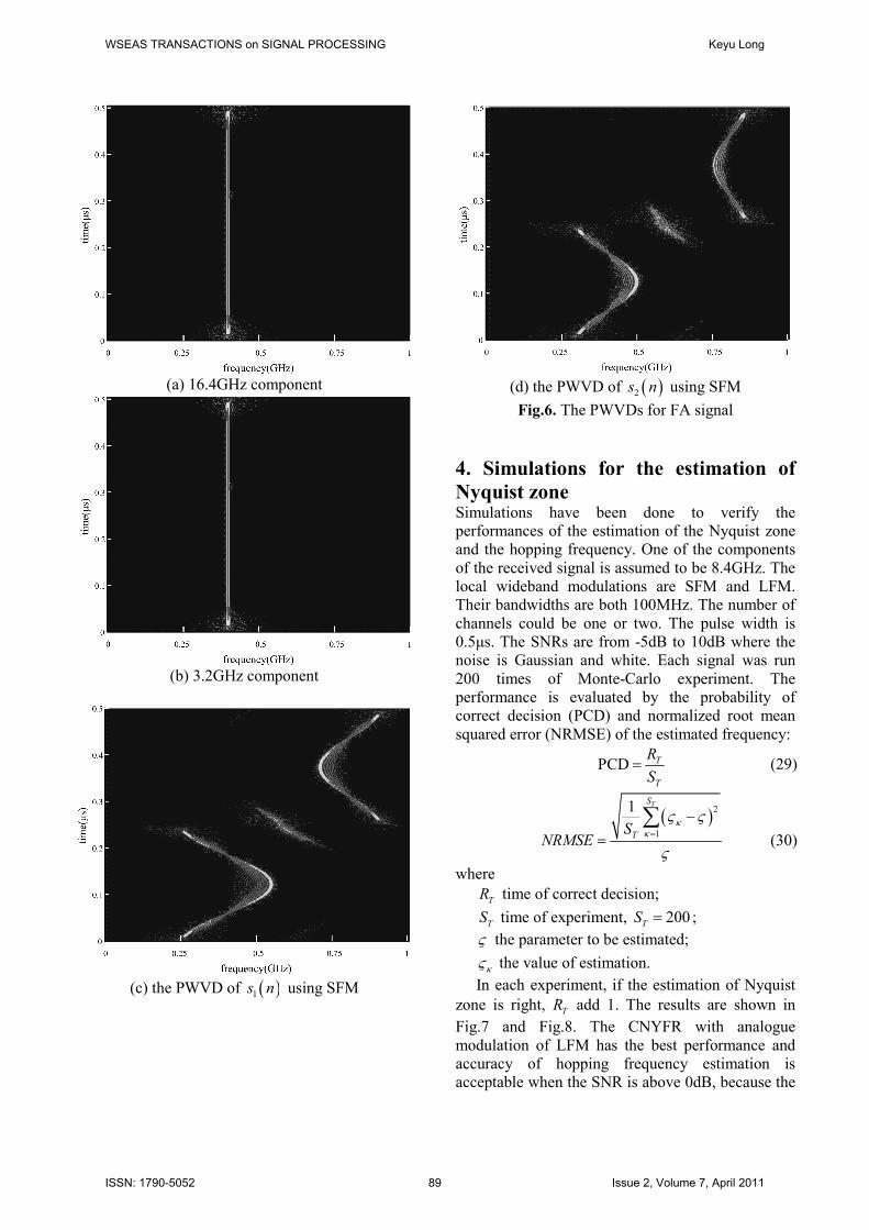
(a) 16.4GHz component
(b) 3.2GHz component
(c) the PWVD of ( )1s n using SFM
(d) the PWVD of ( )2s n using SFM
Fig.6. The PWVDs for FA signal
4. Simulations for the estimation of
Nyquist zone Simulations have been done to verify the
performances of the estimation of the Nyquist zone
and the hopping frequency. One of the components
of the received signal is assumed to be 8.4GHz. The
local wideband modulations are SFM and LFM.
Their bandwidths are both 100MHz. The number of
channels could be one or two. The pulse width is
0.5µs. The SNRs are from -5dB to 10dB where the
noise is Gaussian and white. Each signal was run
200 times of Monte-Carlo experiment. The
performance is evaluated by the probability of
correct decision (PCD) and normalized root mean
squared error (NRMSE) of the estimated frequency:
PCD T
T
R
S= (29)
( )21
1 TS
TSNRMSE
κκ
ς ς
ς=
−
=∑
(30)
where
TR time of correct decision;
TS time of experiment, 200TS = ;
ς the parameter to be estimated;
κς the value of estimation.
In each experiment, if the estimation of Nyquist
zone is right, TR add 1. The results are shown in
Fig.7 and Fig.8. The CNYFR with analogue
modulation of LFM has the best performance and
accuracy of hopping frequency estimation is
acceptable when the SNR is above 0dB, because the
WSEAS TRANSACTIONS on SIGNAL PROCESSING Keyu Long
ISSN: 1790-5052 89 Issue 2, Volume 7, April 2011
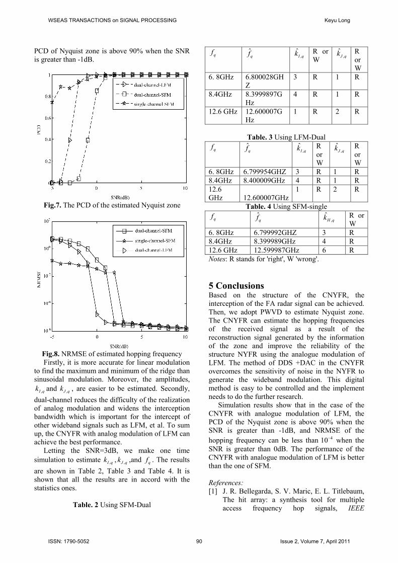
PCD of Nyquist zone is above 90% when the SNR
is greater than -1dB.
Fig.7. The PCD of the estimated Nyquist zone
Fig.8. NRMSE of estimated hopping frequency
Firstly, it is more accurate for linear modulation
to find the maximum and minimum of the ridge than
sinusoidal modulation. Moreover, the amplitudes,
,I qk and ,J qk , are easier to be estimated. Secondly,
dual-channel reduces the difficulty of the realization
of analog modulation and widens the interception
bandwidth which is important for the intercept of
other wideband signals such as LFM, et al. To sum
up, the CNYFR with analog modulation of LFM can
achieve the best performance.
Letting the SNR=3dB, we make one time
simulation to estimate ,I qk , ,J qk ,and qf . The results
are shown in Table 2, Table 3 and Table 4. It is
shown that all the results are in accord with the
statistics ones.
Table. 2 Using SFM-Dual
qf ˆqf ,
ˆI qk R or
W ,
ˆJ qk
R
or
W
6. 8GHz 6.800028GH
Z
3 R 1 R
8.4GHz 8.3999897G
Hz
4 R 1 R
12.6 GHz 12.600007G
Hz
1 R 2 R
Table. 3 Using LFM-Dual
qf ˆqf ,
ˆI qk R
or
W
,ˆJ qk R
or
W
6. 8GHz 6.799954GHZ 3 R 1 R
8.4GHz 8.400009GHz 4 R 1 R
12.6
GHz
12.600007GHz
1 R 2 R
Table. 4 Using SFM-single
qf ˆqf ,
ˆH qk R or
W
6. 8GHz 6.799992GHZ 3 R
8.4GHz 8.399989GHz 4 R
12.6 GHz 12.599987GHz 6 R
Notes: R stands for 'right', W 'wrong'.
5 Conclusions Based on the structure of the CNYFR, the
interception of the FA radar signal can be achieved.
Then, we adopt PWVD to estimate Nyquist zone.
The CNYFR can estimate the hopping frequencies
of the received signal as a result of the
reconstruction signal generated by the information
of the zone and improve the reliability of the
structure NYFR using the analogue modulation of
LFM. The method of DDS +DAC in the CNYFR
overcomes the sensitivity of noise in the NYFR to
generate the wideband modulation. This digital
method is easy to be controlled and the implement
needs to do the further research.
Simulation results show that in the case of the
CNYFR with analogue modulation of LFM, the
PCD of the Nyquist zone is above 90% when the
SNR is greater than -1dB, and NRMSE of the
hopping frequency can be less than 410− when the
SNR is greater than 0dB. The performance of the
CNYFR with analogue modulation of LFM is better
than the one of SFM.
References:
[1] J. R. Bellegarda, S. V. Maric, E. L. Titlebaum,
The hit array: a synthesis tool for multiple
access frequency hop signals, IEEE
WSEAS TRANSACTIONS on SIGNAL PROCESSING Keyu Long
ISSN: 1790-5052 90 Issue 2, Volume 7, April 2011
Transactions on Aerospace and Electronic
Systems, Vol.29, No.3, 1993, pp.624-635.
[2] K. Morrison, Effective bandwidth SF-CW SAR
increase using frequency agility, IEEE
Aerospace and Electronic Systems Magazine, ,
Vol.21, No.6, 2006, pp.28-32.
[3] K. Becker, Passive localization of frequency-
agile radars from angle and frequency
measurements, IEEE Transactions on
Aerospace and Electronic Systems, Vol.35,
No.4, 1999, pp.1129-1144.
[4] S. R. Rogers, On analytical evaluation of glint
error reduction for frequency-hopping radars,
IEEE Transactions on Aerospace and
Electronic Systems, Vol.27, No.6, 1991, pp.
891-894.
[5] G. Lellouch, P. Tran, R. Pribic, P. van
Genderen, OFDM waveforms for frequency
agility and opportunities for doppler processing
in radar, IEEE Radar Conference, 2008.
[6] E. J. Candes, T. Tao, Near-optimal signal
recovery from random projections: universal
encoding strategies? IEEE Transactions on
Information Theory, Vol.52, No.12, 2006, pp.
5406-5425.
[7] D. L. Donoho, Compressed sensing, IEEE
Transactions on Information Theory, Vol.52,
No.4, 2006, pp. 1289-1306.
[8] M. A. Herman, T. Strohmer, High-resolution
radar via compressed sensing, IEEE
Transactions on Signal Processing, Vol.57,
No.6, 2009, pp. 2275-2284.
[9] J. Ma, Compressed sensing for surface
characterization and metrology. IEEE
Transactions on Instrumentation and
Measurement, Vol.59, No.6, 2010, pp. 1600-
1615.
[10] L. C. Potter, E. Ertin, J. T. Parker, M. Cetin,
Sparsity and compressed sensing in radar
imaging. IEEE Proceedings, Vol.98, No.6,
2010, pp. 1006-1020.
[11] J. Provost, F. Lesage, The application of
compressed sensing for photo-acoustic
tomography. IEEE Transactions on Medical
Imaging, Vol.28, No.4, 2009, pp. 585-594.
[12] P. Flandrin, P. Borgnat, Time-frequency energy
distributions meet compressed sensing, IEEE
Transactions on Signal Processing, Vol.58,
No.6, 2010, pp. 2974-2982.
[13] J. A. Tropp, J. N. Laska, M. F. Duarte, J. K.
Romberg, R. G. Baraniuk, Beyond Nyquist:
efficient sampling of sparse bandlimited signals,
IEEE Transactions on information theory, Vol.
56, No. 1, 2010, pp. 520-544.
[14] J. N. Laska, S. Kirolos, M. F. Duarte, T. S.
Ragheb, R. G. Baraniuk, Y. Massoud, Theory
and implementation of an analog-to-
information converter using random
demodulation, IEEE International Symposium
on Circuits and Systems, 2007, pp. 1959 – 1962.
[15] J. Romberg. Compressive sensing by random
convolution. 2nd IEEE International Workshop
on Computational Advances in Multi-Sensor
Adaptive Processing, 2007, pp. 137 – 140.
[16] J. A. Tropp, M. B. Wakin, M. F. Duarte, D.
Baron, R. G. Baraniuk, Random filters for
compressive sampling and reconstruction,
IEEE International Conference on Acoustics,
Speech and Signal Processing, 2006, pp. III.
[17] D. Takhar, J. N. Laska, M. Wakin, M. F.
Duarte, D. Baron, S. Sarvotham, K. F. Kelly, R.
G. Baraniuk, A new compressive imaging
camera architecture using optical-domain
compression, Computational Imaging, 2006.
[18] G. L. Fudge, R. E. Bland, M. A. Chivers, S.
Ravindran, J. Haupt, P. E. Pace, A Nyquist
folding analog-to-information receiver, 42nd
Asilomar Conference on Signals, Systems and
Computers, 2008, pp. 541-545.
WSEAS TRANSACTIONS on SIGNAL PROCESSING Keyu Long
ISSN: 1790-5052 91 Issue 2, Volume 7, April 2011