1

Interactive Learning of Temporal Features forControl

Rodrigo Pérez-Dattari1, Carlos Celemin1, Giovanni Franzese1, Javier Ruiz-del-Solar2 and Jens Kober1

I. INTRODUCTION

The ongoing industry revolution is demanding more flexi-ble products, including robots in household environments ormedium scale factories. Such robots should be able to adaptto new conditions and environments, and to be programmedwith ease. As an example, let us suppose that there are robotmanipulators working in an industrial production line that needto perform a new task. If these robots were hard coded, it couldtake days to adapt them to the new settings, which would stopthe production of the factory. Easily programmable robots bynon-expert humans would speed up this process considerably.

In this regard, we present a framework in which robots arecapable to quickly learn new control policies and state repre-sentations, by using occasional corrective human feedback. Toachieve this, we focus on interactively learning these policiesfrom non-expert humans that act as teachers.

We present a Neural Network (NN) architecture, alongwith an Interactive Imitation Learning (IIL) method, whichefficiently learns spatiotemporal features and policies from rawhigh dimensional observations (raw pixels from an image), fortasks in environments not fully temporally observable.

We denominate IIL as a branch of Imitation Learning (IL)where human teachers provide different kinds of feedback tothe robots, like new demonstrations triggered by robot queries[1], corrections [2], preferences [3], reinforcements [4], etc.Most IL methods work under the assumption of learning fromperfect demonstrations; therefore, they fail when teachers onlyhave partial insights in the task execution. Non-expert teacherscould be considered all the users who are neither MachineLearning (ML)/control experts, nor skilled to fully show thedesired behavior of the policy.

Interactive approaches like COACH [5], and some Inter-active Reinforcement Learning (IRL) approaches [4], [6],are intended for non-expert teachers, but are not completelydeployable for end-users. Sequential decision-making learningmethods (IL, IIL, IRL, etc.) rely on good state representations,which make the shaping of the policy landscape simple,and provide good generalization properties. However, thisrequirement brings the need of experts on feature engineeringto pre-process the states properly, before running the learningalgorithms.

1R. Pérez-Dattari, C. Celemin, G. Franzese and J. Kober are withthe Department of Cognitive Robotics, Delft University of Technology,Delft, The Netherlands e-mail: (r.j.perezdattari, c.e.celeminpaez, g.franzese,j.kober)@tudelft.nl.

2J. Ruiz-Del-Solar is with the Department of Electrical Eng. and theAdvanced Mining Technology Center, Universidad de Chile, Chile e-mail:jruizd@ing.uchile.cl.

Environment

Agent

Teacher

action !

feedback !

World Model

observation !

Fig. 1: Interactively shaping policies with agents that modelthe world.

The inclusion of Deep Learning (DL) in IL (given itspopularity gained in the field of Reinforcement Learning (RL)[7]), allows to skip pre-processing modules for the input of thepolicies, since some architectures of NNs endow the agentswith intrinsic feature extraction capabilities. This has beenexhaustively tested in end-to-end settings [7]. In this regard,DL allows non-expert humans to shape policies based only ontheir feedback.

Nevertheless, in real-world problems, we commonly facetasks wherein the observations do not explain the completestate of the agent due to the lack of temporal information (e.g.rates of change), or because the agent-environment interactionis non-Markovian (e.g. dealing with occlusions). For thesecases, it is necessary to provide memory to the learningpolicy. Recurrent Neural Networks (RNNs) can learn to modeldependencies on the past, and map them to the current outputs.This recurrency has been used in RL and IL mostly using LongShort-Term Memory (LSTM) networks [8].

Therefore, LSTMs are included in our NN architecture tolearn temporal features, which contain relevant informationfrom the past. However, DL algorithms require large amountsof data, so as a way to tackle this shortcoming, State Repre-sentation Learning (SRL) has been used to learn features moreefficiently [9], [10]. Considering that real robots and humanusers have time limitations, as an SRL strategy, a model ofthe world is learned to obtain state representations that makethe policy convergence possible within feasible training time

IEEE Robotics and Automation Magazine 2020

2

intervals (see Fig. 1).The combination of SRL and the teacher’s feedback is a

powerful strategy to efficiently learn temporal features fromraw observations in non-Markovian environments.

The experiments presented in this paper show the im-pact of the proposed architecture in terms of data effi-ciency and policy final performance within the Deep COACH(D-COACH) IIL framework [11]. Additionally, the experi-mental procedure shows that the proposed architecture couldbe even used with other IL methods, such as Data Aggre-gation (DAgger) [12]. The code used in this paper can befound at: https://github.com/rperezdattari/Interactive-Learning-of-Temporal-Features-for-Control.

The paper is organized as follows: background on ap-proaches used within our proposed method, and the relatedwork are presented in Section II. Section III describes theproposed NN architecture along with the learning method.Experiments and results are given in Section IV, and finallythe conclusions are drawn in Section V.

II. BACKGROUND AND RELATED WORK

Our method combines elements from SRL, IL and mem-ory in NN models to build a framework that enablesnon-expert teachers to interactively shape policies in tasks withnon-Markovian environments. These elements are introducedhereunder.

A. Dealing with non-Markovian Environments

There are different reasons why a process could be par-tially observable. One of them is when the state describestime-dependent phenomena, but the observation only con-tains partial information of it. For instance, velocities cannotbe estimated from camera images unless observations fromdifferent time steps are combined. Other examples of time-dependent phenomena are temporary occlusions or corruptedcommunication systems between the sensors and the agent.

For these environments, the temporal information needs tobe implicitly obtained within the policy model. There aretwo well-known approaches for adding memory to agentsin sequential decision-making problems when using NNs asfunction approximators:

1) Observation stacking policies [13]: stacking the last Nobservations (ot, ot−1, ...oN ), and using this stack as theinput of the network.

2) Recurrent policies [14]: including RNN layers in thepolicy architecture.

One of the main issues of observation stacking is that thememory of these models is determined by the number ofstacked observations. The overhead increase rapidly for largersequences in high-dimensional observation problems.

In contrast, RNNs have the ability to model informationfor an arbitrarily long amount of time [15]. Also, they do notadd input-related overheads, because when these models areevaluated, they only use the last observation. Therefore, RNNshave lower computational cost than observation stacking.Given the more practical usage of recurrent models and their

capability of representing arbitrarily long sequences, in thiswork we use RNN-based policies (with LSTM layers) in theproposed NN architecture.

Nevertheless, the use of LSTMs has a critical disadvantage,since its training is more complex and requires more data,something very problematic when considering human teachersand real systems. We will now introduce SRL, which helps toaccelerate the LSTM converge.

B. State Representation Learning

In most of the problems faced in robotics, the state st, whichfully describes the situation of the environment at time stept, is not fully accessible from the robot’s observation ot.As mentioned before, in several problems the observationslack temporal information required in the state description.Evenmore, these observations tend to be raw sensor mea-surements that can be high-dimensional, highly redundant andambiguous. A portion of this data may even be irrelevant.

As a consequence, to successfully solve these problems apolicy needs to 1) find temporal correlations between severalconsecutive observations, and 2) extract relevant features fromobservations that are hard to interpret. However, finding rela-tions between these large data structures with the underlyingphenomena of the environment, while learning controllers, canbe extremely inefficient. Therefore, efficiently building con-trollers on top of raw observations requires to learn informativelow-dimensional state representations [16]. The objective ofSRL is to obtain an observer capable of generating suchrepresentations.

A compact representation of a state is considered to besuitable for control if the resulting state representation:

• is Markovian,• has good generalization to unseen states, and• is defined in low dimensional space (considerably lower

than the actual observation dimensionality) [9].Along with the control objective function (e.g. reward

function, imitation cost function), other objective functions canbe used for SRL [10], namely:

• observation reconstruction,• forward model or next observation prediction,• inverse model,• reward function, or• value function.

C. Interactive Learning methods

This subsection introduces briefly two approaches for interac-tively learning from human teachers while agents are executingthe task.

1) Data Aggregation: (HG-)DAgger

DAgger [12] is an IIL algorithm that aims to collect data withonline sampling. To achieve this, trajectories are generated bycombining the agent’s policy πθ and the expert’s policy. Theobservations ot and the demonstrator’s corresponding actions

3

Algorithm 1 (HG-)DAgger

1: Require: demonstrations database D with initial demon-strations, policy update frequency b

2: for t = 1,2,... do3: if mod(t, b) is 0 then4: update πθ from D5: observe state ot6: select action from agent or expert7: execute action8: feedback provide label a∗t for ot, if necessary9: aggregate (ot, a

∗t ) to D

a∗t are paired and added to a database D, which is used fortraining the policy’s parameters θ iteratively in a supervisedlearning manner, in order to asymptotically approach theexpert’s policy. At the beginning of the learning process, thedemonstrator has all the influence over the trajectory made bythe agent; then, the probability of following the demonstrator’sactions decays exponentially.

For working in real-world systems, with humans asdemonstrators, a variation of DAgger, Human-Gated DAg-ger (HG-DAgger) [2], was introduced. In this approach, thedemonstrator is not expected to give labels over every actionof the agent, but only in places where s/he considers thatthe agent’s policy needs improvement. Only these labels areaggregated to the database and used for updating the policy.Additionally, every time feedback is given by the human, thepolicy will follow the provided action. As a safety measure, inHG-DAgger the uncertainty of the policy over the observationspace is estimated; this element is omitted in this work.Algorithm 1 shows the general structure of DAgger and HG-DAgger.

2) Deep COACH

In this framework [11], humans shape policies giving occa-sional corrective feedback over the actions executed by theagents. If an agent takes an action that the human considersto be erroneous, then s/he would indicate with a binary signalht, the direction in which the action should be modified.

This feedback is used to generate an error signal for updat-ing the policy parameters θ. It is done in a supervised learningmanner with the cost function J using the mean squared errorand stochastic gradient descent. Hence, the update rule is:

θ ← θ − α · ∇θJ(θ). (1)

The feedback given by the human only indicates the signof the policy error. Its magnitude is supposed to be unknown,since the algorithm works under the assumption that the useris non-expert; therefore, s/he does not know the magnitude ofthe proper action. Instead, the error magnitude is defined asthe hyperparameter e, that must be defined before starting thelearning process. Thus, the policy errort is defined by ht · e.

To compute a gradient in the parameter space of the policy,the error needs to be a function of θ. This is achieved byobserving that:

Algorithm 2 Deep COACH

1: Require: error magnitude e, buffer update interval b2: Init: B = [] # initialize memory buffer3: for t = 1,2,... do4: observe state ot5: execute action at = πθ(ot)6: feedback human corrective advice ht7: if ht is not 0 then8: error t = ht · e9: atarget(t) = at + error t

10: update π using SGD with pair (ot, atargett )

11: update π using SGD with a mini-batch sampledfrom B

12: append (ot, atargett ) to B

13: if mod(t, b) is 0 then14: update πθ using SGD with a mini-batch sampled

from B

errort(θ) = atargett − πθ(ot) (2)

where atargett is the incremental objective generated by the

feedback of the human atargett = at + errort and at is the

current output of the policy πθ. From Equations (1), (2),and the derivative of the mean squared error, we can get theCOACH update step:

θ ← θ + α · errort · ∇θπθ. (3)

To be more data efficient and to avoid locally over-fittingto the most recent corrections, Deep COACH has a memorybuffer that stores the tuple (ot, a

targett ) and replays this informa-

tion during learning. Additionally, when working in problemswith high-dimensional observations, an autoencoding cost isincorporated in Deep COACH as an observation reconstructionSRL strategy. In the Deep COACH pseudo-code (Algorithm2) this SRL step is omitted. Deep COACH learns everythingfrom scratch in only one interactive phase, unlike other deepinteractive RL approaches [4], [6], which split the learningprocess into two sequential learning phases. First, recordingsamples of the environment for training a dimensionalityreduction model (e.g. an autoencoder); secondly, using thatmodel for the input of the policy network during the actualinteractive learning process.

III. LEARNING TEMPORAL FEATURES BASED ONINTERACTIVE TEACHING AND WORLD MODELLING

In this section, the SRL NN architecture is described alongwith the interactive algorithm for policy shaping.

A. Network Architecture for Extracting Temporal Features

For approaching problems that lack temporal information inthe observations, the most common solution is to model thepolicy with RNNs as discussed in Section II-A; therefore, wepropose to shape policies that are built on top of RNNs, with

4

Policy

Transition

Model !"#$

!"

%"

%"

&'(

)"*$+,-.

)"+,-.

Fig. 2: Transition model and policy general structure.

occasional human feedback. In this work, we are using theterms world model and transition model interchangeably.

IIL methods can take advantage of SRL for training withother objective functions by 1) making use of all the experi-ence collected in every time step, and 2) boosting the processof finding compact Markovian embeddings. We propose tohave a neural architecture separated into two parts: 1) transi-tion model, and 2) policy. The transition model is in chargeof learning the dynamics of the environment in a supervisedmanner using samples collected by the agent. The policy partis shaped only using corrective feedback. Figure 2 shows adiagram of this architecture.

Learning to predict the next observation ot+1 forces aMarkovian state representation. This has been successfullyapplied in RL [17]. RNNs can encode information frompast observations in their hidden state hLSTM

t . Thus, theobjective of the first part of the neural network is to learnM(ot, at, h

LSTMt−1 ) = ot+1, which, as a consequence, learns

to embed past observations in hLSTMt . Additionally, when the

observations are high-dimensional (raw images), the agentsalso need to learn to compress spatial information. To achievethis, a common approach is to compress this information inthe latent space of an autoencoder.

For the first part of the architecture, we propose to usethe combination of an autoencoder with an LSTM to com-pute the transition function model, i.e., predicting the nexthigh-dimensional observation. A detailed diagram of this ar-chitecture can be seen in Figure 3.

In the second part of the architecture, the policy takes asinput, a representation of the state st, that is generated insidethe transition model network. This representation is obtainedat the output of a fully-connected layer (FC3), that combinesthe information of hLSTM

t−1 with the encoder compression ofthe current observation e(ot). This is achieved by adding askipping connection between the output of the encoder andthe output of the LSTM.

B. Interactive Algorithm for Policy and World-Model Learn-ing

In Algorithm 3, the pseudo-code of the state representationlearning strategy is presented. The hidden state of the LSTMis denoted as hLSTM, and the human corrective feedback as

h. In every time step, a buffer D stores the samples of thetransitions with sequences of length τ (line 5). The agentexecutes an action based on its last observation and the currenthidden state of the LSTM (line 6). This hidden state is updatedusing its previous value and the most recent observation andaction (line 7). Line 8 captures the occasional feedback ofthe teacher, which could be a relative correction when usingDeep COACH, or the corrective demonstration when usingHG-DAgger. Also, depending on the learning algorithm, thepolicy is updated in different ways (line 9) .D replays past transitions of the environment in order to

update the transition function model (line 11). This is donefollowing the bootstrapped random updates [14] strategy. Thismodel is updated every d time steps.

Algorithm 3 Online Temporal Feature Learning

1: Require: Policy update algorithm πupdate, training se-quence length τ , model update rate d

2: Init: D = []3: for t = 1,2,... do4: observe observation ot5: append (ot−1, ..., ot−τ , at−1, ..., at−τ , ot) to D6: execute action at = πθ(ot, h

LSTMt−1 )

7: compute hLSTMt from M(ot, at, h

LSTMt−1 )

8: feedback human feedback ht9: call πupdate(ot, at, ht)

10: if mod(t, d) is 0 then11: update M using SGD with mini-batches of se-

quences sampled from D

IV. EXPERIMENTS AND RESULTS

In this section, experiments for validating the proposed neuralnetwork architecture and the interactive training algorithm arepresented. In order to obtain a thorough evaluation, differentexperiments are carried out to compare and measure theperformance (return i.e. sum of rewards) of the proposedcomponents. Initially, the network architecture based on SRLis evaluated in an ablation study, aiming to quantify the dataefficiency improvement added by its different components.Then, using the proposed architecture, D-COACH is comparedwith (HG-)DAgger using simulated tasks and simulated teach-ers (oracles). The third set of experiments is carried out withhuman teachers in simulated environments, again comparingdifferent learning methods. Finally, a fourth set of validationexperiments is carried out in real systems with human teachers.Most of the results are presented in this paper; however, someof them are in the supplementary material, along with moredetailed information on the experiments

Two real and three simulated environments with differentcomplexity levels were used, all of them using raw images asobservations. The simulated environments are Mountain-Car,Swing-Up Pendulum, and Car Racing, whose implementationsare taken from OpenAI Gym [18]. These simulations providerendered image frames as observations of the environment.These frames visually describe the position of the system but

5

Convolution:

Deconvolution:

Reshape:

Normalization:

Fully-connected:

Recurrent:

Identity:

Concatenate:

!" !#$

Encoder Decoder

Policy

%( !)

"!

"!

C1

FC5 FC6 FC7

Transition Model

FC4

Memory

FC2

R1 FC3

CC1

FC1C2 C3

DC1 DC2 DC3N1 N2

N3 N4

#$%

CC2

&!'(*+

&!,-'(*+

Fig. 3: Proposed neural network architecture. Convolutional and recurrent (LSTM) layers are included in the transition modelin order to learn spatiotemporal state representations. The estimated state st is used as input to the policy, which is a fully-connected NN.

not its velocity, which is necessary to control the system.The experiments on the real physical systems consist of aSwing-Up Pendulum and a setup for picking oranges on aconveyor belt with a 3 degrees of freedom (DoF) robot arm.

The metrics used for the comparisons are the achieved finalpolicy performance, and the speed of convergence, which isvery relevant when dealing with both, real systems and humanteachers. A video showing most of these experiments can befound at: youtu.be/4kWGfNdm21A.

A. Ablation study

In this ablation study, the architecture of the network isthe independent variable of the study. Three independentcomparisons were carried out using DAgger, HG-DAgger andD-COACH. The training sessions were run using a simulatedteacher to avoid any influence of human factors.

Three different architectures were tested for learning thepolicy from an oracle. The structure of the networks isintroduced below:

1) Full network: Proposed architecture.2) Memoryless state representation learning (M-less

SRL): Similar to the full network, but without usingrecurrence between the encoder and decoder. The au-toencoder is trained using the reconstruction error of theobservation.

3) Direct policy learning (DPL): Same architecture as inthe full network, but without using SRL, i.e., not trainingthe transition model. The encoding, recurrent layers andpolicy are trained only using the cost of the policy.

The ablation study is done on a modified version of the CarRacing environment. Normally, this environment provides anupper view of a car in a racing track. In this case, we occludedthe bottom half of this observation, such that the agent is notable to precisely know its position in the track. This positioncan be estimated if past observations are taken into account.As a consequence, this is an appropriate setting for makinga comparison of different neural network architectures. Table

I shows the different performances obtained by the learningalgorithms when modifying the structure of the network. Theseresults show a normalized averaged return over 10 repetitionsfor each experiment, in which 5 evaluations were carried foreach one of these repetitions.

TABLE I: Performance (return) comparison of different learn-ing methods in the Car Racing problem. Returns were nor-malized with respect to the best performance (DAgger Full).

FULL M-less SRL DPLD-COACH 0.97 0.76 0.68DAgger 1.00 0.87 0.96HG-DAgger 0.89 0.69 0.90

As expected, DAgger with the Full architecture obtainedthe best performance, and given that it receives new samplesevery time step, it was robust against the changes in thearchitecture, even when it did not have memory. On the otherhand, D-COACH was very sensitive to the changes in thearchitecture, especially with the DPL architecture. This showshow the Full model is able to enhance the performance of theagents in problems where temporal information is required. Iteven makes Deep COACH perform almost as well as DAgger,despite that the former does not require constant and perfectteacher feedback. Finally, HG-DAgger was more robust thanD-COACH in the DPL case, but its performance with the fullmodel was not as good.

B. Simulated tasks with simulated teachers

In the second set of experiments, a comparison betweenthe algorithms DAgger, HG-DAgger, and Deep COACH wascarried out using the proposed Full network architecture. Tokeep the experiments free from human factor effects, theteaching process was, once again, performed with simulatedteachers. The methods were tested in the simulated problemsMountain Car (in the supplementary material), and Swing-UpPendulum. A mean of the return obtained over 20 repetitions

6

0 1000 2000 3000 4000 5000 6000 7000Time step

−3500

−3000

−2500

−2000

−1500

−1000

−500

Return

Simulated Swing-Up Pendulum Learning Curve

Oracle

Random policy

D-COACH

DAgger

HG-DAgger

0 1 2 3 4 5 6 7 8 9 10 11Time (min)

Fig. 4: D-COACH and (HG-)DAgger comparison in theSwing-Up Pendulum problem using a simulated teacher.

is presented for these experiments, along with the maximumand minimum values of these distributions.

Swing-Up Pendulum

In the case of the Swing-Up Pendulum, the results are verydifferent for both DAgger agents (see Fig. 4). Both havea higher rate of improvement than Deep COACH duringthe first minutes, when the policy is learning the swingingbehavior. Since the swinging part requires large actions, theimprovement with Deep COACH is slower. However, oncethe policy is able to swing the pendulum up, the second partof the task is to keep the balance in the upright position,which requires fine actions. It is at this point when learningbecomes easier for the Deep COACH agent, which obtains aconstant and faster improvement than the HG-DAgger agent,even reaching a higher performance. In Fig. 4, the expectedperformance upper bound is showed with a black dashed line,which is the return obtained by the simulated teacher. Thepurple dashed line shows the performance of a random policy,which is the expected lower bound.

C. Simulated tasks with human teachers

The previous experiments give insights into how the policyarchitectures and/or the learning methods perform when im-itating an oracle. Most IL methods are intended for learningfrom any source of expert demonstrations. It does not have tobe a human necessarily; it can be any type of agent. However,the scope of this work is on learning from non-expert humanteachers, who are complex to model and simulate. Therefore,conclusions have to be based on results that also includevalidation with real users.

Experiments with the Mountain-Car (in the supplementarymaterial), and the Swing-Up Pendulum were run with 8 humanteachers. In this case, the classical DAgger approach is notused, since, as discussed in Section II-C, it is not specificallydesigned for human users. Instead, HG-DAgger is validated.

0 2000 4000 6000 8000 10000Time step

−3500

−3000

−2500

−2000

−1500

−1000

−500

Return

Simulated Swing-Up Pendulum Learning Curve w/ Human Teachers

Human (teleoperation)

Random policy

D-COACH

HG-DAgger

0 1 2 3 4 5 6 7 8 9 10 11 12 13 14 15 16Time (min)

Fig. 5: Simulated Swing-Up Pendulum learning curve withhuman teachers

Swing-Up Pendulum

This task is relatively simple from a control theory pointof view. Nevertheless, it is quite challenging for humans totele-operate the pendulum, due to its fast dynamics. Indeed,the participants were not able to successfully tele-operatethe agent; therefore, unlike the Mountain-Car task, we couldconsider the participants as non-experts on the task.

Fig. 5 shows the results of this experiment, which aresimilar to the ones presented in Fig. 4. At the beginning, DeepCOACH has a slower improvement when learning to swingup; however, it learns faster than HG-DAgger when the policyneeds to learn the accurate task of balancing the pendulum.For the users, it is more intuitive and easier to improve thebalancing with the relative corrections of Deep COACH thanwith the perfect corrective demonstrations of HG-DAgger,as they do not need to know the right action, rather justthe direction of the correction. Unlike the performance ofthe simulated teacher depicted in Fig. 4, this plot showsthe performance of the best human teacher tele-operatingthe pendulum with the same interface used for the teachingprocess. It can be seen that using both agents allowed to obtainpolicies that outperform the non-expert human teachers.

All the policies trained with Deep COACH were able tobalance the pendulum, whereas with HG-DAgger the successrate was the half. Additionally, after the experiment, theparticipants were queried about what learning strategy theypreferred. Seven out of eight expressed preference for DeepCOACH.

D. Validation on physical systems with human teachers

The previous experiments performed comparison studies of theNN architectures and the learning methods under controlledconditions in simulated environments. In this section, DeepCOACH is validated with human teachers and real systems intwo different tasks: 1) a real Swing-Up Pendulum, and 2) afruits classifier robot arm.

The real Swing-Up pendulum is a very complex system

7

Fig. 6: Orange selector experimental set-up. 1) conveyor belt,2) “orange” samples, 3) frame observed by the camera, 4)RGB camera, and 5) 3 DoF robot arm.

for a human to tele-operate. Its dynamics are faster than thesimulated one of OpenAI Gym used in the previous experi-ments. The supplementary material provides more details ofthis environment along with the learning curve of the agentstrained by the participants of this validation experiment. Thoseresults, along with the video, show that non-expert teacherscan manage to teach good policies.

Orange selector with a robot arm

This set-up consists of a conveyor belt transporting “pears”and “oranges”, a 3 DoF robot arm located over the belt, andan RGB camera with a top view of the belt. The image ofthe camera does not capture the robot arm. The robot hasto select oranges with the end effector, but avoid pears. Therobot does not have any tool like a gripper or vacuum gripperto pick up the oranges. Therefore, in this context, we considera successful selection of an orange when the end effectorintersects the object. The performance of the learning policyis measured using two indices: 1) rate of oranges successfullyselected, and 2) rate of pears successfully rejected.

The observations obtained by the camera are from a differ-ent region of the conveyor belt than where the robot is acting.Therefore observations cannot be used for compensating therobot position in the current time step, rather they are mean-ingful for future decisions. In other words, the current actionmust be based on past observations. Indeed, the delay betweenthe observations and its influence on the actions is around 1.5seconds. This delay is given by the difference between thetime when the object gets out from the camera range and thetime it reaches the robot’s operating range. This is why thistask requires to learn temporal features for the policy.

The problem is solved by splitting it into two sub-taskswhich are trained separately:

0 2000 4000 6000 8000 10000 12000 14000Time step

0.0

0.2

0.4

0.6

0.8

1.0

Selection/R

ejection

Success

Rate

Orange Selector Learning Curve

Orange Selection

Pear Rejection

0 5 10 15 20 25 30 35 40 45 50Time (min)

Fig. 7: Orange selection/pear rejection learning curve.

1) Orange selection: The robot must intercept the orangecoordinate with the end effector, right when it passesbelow the robot.

2) Pear rejection: The robot must classify between or-anges and pears, so when a pear is approaching underthe robot, the end effector should be lifted far from thebelt plane, otherwise it should get close.

These two sub-tasks can be trained sequentially. The orangeselection is trained initially, with a procedure in which thereare some oranges being transported by the belt with fixedpositions, while some others are placed randomly. This inorder to avoid over-fitting of the policy to specific sequences.

When the robot is able to track the oranges in its reach,the pear rejection learning starts. For that, pears are placedrandomly throughout the sequences of oranges, and the humanteacher advises corrections on the robot movement in order tomake the end effector move away from the pears when theyare in the operation region of the robot.

Fig. 7 depicts the average learning curves for this task after5 runs of the teaching process. It is possible to see that thepear rejection sub-task is learned within 20 minutes with 100%success, while the orange selection is a harder sub-task thatonly reaches around 80% success after 50 minutes. Effectively,combining the two sub-tasks, the performance of the learnedpolicies is given only by the success of the orange selection,since the pear rejection was perfectly attained in all the runsexecuted for this experiment.

V. CONCLUSION

This paper has introduced and validated a SRL strategy forlearning policies interactively from human teachers in envi-ronments not fully temporally observable. Results show thatwhen meaningful spatiotemporal features are extracted, it ispossible to teach complex end-to-end policies to agents usingjust occasional, relative, and binary corrective signals. Evenmore, these policies can be learned from teachers who are notskilled to execute the task.

The evaluations with the Data Aggregation approaches andDeep COACH depict the potential of this kind of architecture

8

to work on different IIL methods. Especially in methods basedon occasional feedback, which are intended to reduce thehuman workload.

The comparative results between HG-DAgger and DeepCOACH with non-expert teachers showed that with the former,the policy will remain biased with mistaken samples evenif the teacher makes sure of not providing more wrongcorrections (given that it works with the assumption of expertdemonstrations); hence, it makes harder to refine the policy.On the other hand, Deep COACH proved to be more robustto mistaken corrections given by humans, since all the non-expert users were able to teach tasks that they were not ableto demonstrate.

The previous mentioned shortcoming of DAgger algorithmsopen possibilities for future works, which are intended to studyhow to deal with databases with mistaken examples. Anotherfield of study is the one of data-efficient movement generationin animation [19], which combined with our method, wouldmake it possible to learn (non-)periodic movements using spa-tiotemporal features and IIL. Challenges such as the generationof smooth, precise, and stylistic movements (i.e. dealing withhigh-frequency details [20]) could be also addressed.

ACKNOWLEDGMENT

This research has been funded by the Netherlands Organizationfor Scientific Research (NWO) project FlexCRAFT, grantnumber P17-01, by the ERC Stg TERI, project reference#804907, by FONDECYT project [1201170], and by CON-ICYT project [AFB180004].

REFERENCES

[1] S. Chernova and M. Veloso, “Interactive policy learning throughconfidence-based autonomy,” Journal of Artificial Intelligence Research,vol. 34, pp. 1–25, 2009.

[2] M. Kelly, C. Sidrane, K. Driggs-Campbell, and M. Kochenderfer, “Hg-dagger: Interactive imitation learning with human experts,” in 2019International Conference on Robotics and Automation (ICRA). IEEE,2019, pp. 8077–8083.

[3] P. F. Christiano, J. Leike, T. Brown, M. Martic, S. Legg, and D. Amodei,“Deep reinforcement learning from human preferences,” in Advances inNeural Information Processing Systems, 2017, pp. 4299–4307.

[4] W. B. Knox and P. Stone, “Interactively shaping agents via human rein-forcement: The TAMER framework,” in Fifth International Conferenceon Knowledge Capture. ACM, 2009, pp. 9–16.

[5] C. Celemin and J. Ruiz-del Solar, “An interactive framework for learningcontinuous actions policies based on corrective feedback,” Journal ofIntelligent & Robotic Systems, pp. 1–21, 2018.

[6] J. MacGlashan, M. K. Ho, R. Loftin, B. Peng, G. Wang, D. L.Roberts, M. E. Taylor, and M. L. Littman, “Interactive learning frompolicy-dependent human feedback,” in 34th International Conferenceon Machine Learning - Volume 70. JMLR. org, 2017, pp. 2285–2294.

[7] V. Mnih, K. Kavukcuoglu, D. Silver, A. A. Rusu, J. Veness, M. G.Bellemare, A. Graves, M. Riedmiller, A. K. Fidjeland, G. Ostrovskiet al., “Human-level control through deep reinforcement learning,”Nature, vol. 518, no. 7540, p. 529, 2015.

[8] S. Hochreiter and J. Schmidhuber, “Long short-term memory,” NeuralComputation, vol. 9, no. 8, pp. 1735–1780, 1997.

[9] W. Böhmer, J. T. Springenberg, J. Boedecker, M. Riedmiller, andK. Obermayer, “Autonomous learning of state representations for con-trol: An emerging field aims to autonomously learn state representationsfor reinforcement learning agents from their real-world sensor observa-tions,” KI-Künstliche Intelligenz, vol. 29, no. 4, pp. 353–362, 2015.

[10] T. Lesort, N. Díaz-Rodríguez, J.-F. Goudou, and D. Filliat, “Staterepresentation learning for control: An overview,” Neural Networks, vol.108, pp. 379–392, 2018.

[11] R. Pérez-Dattari, C. Celemin, J. Ruiz-del Solar, and J. Kober, “Contin-uous control for high-dimensional state spaces: An interactive learningapproach,” in 2019 International Conference on Robotics and Automa-tion (ICRA). IEEE, 2019, pp. 7611–7617.

[12] S. Ross, G. Gordon, and D. Bagnell, “A reduction of imitation learningand structured prediction to no-regret online learning,” in FourteenthInternational Conference on Artificial Intelligence and Statistics, 2011,pp. 627–635.

[13] V. Mnih, K. Kavukcuoglu, D. Silver, A. A. Rusu, J. Veness, M. G.Bellemare, A. Graves, M. Riedmiller, A. K. Fidjeland, G. Ostrovskiet al., “Human-level control through deep reinforcement learning,”Nature, vol. 518, no. 7540, p. 529, 2015.

[14] M. Hausknecht and P. Stone, “Deep recurrent Q-learning for partiallyobservable MDPs,” in 2015 AAAI Fall Symposium Series, 2015.

[15] G. Lample and D. S. Chaplot, “Playing fps games with deep re-inforcement learning,” in Thirty-First AAAI Conference on ArtificialIntelligence, 2017.

[16] D. Ha and J. Schmidhuber, “Recurrent world models facilitate policyevolution,” in Advances in Neural Information Processing Systems, 2018,pp. 2450–2462.

[17] A. Zhang, H. Satija, and J. Pineau, “Decoupling dynamics and rewardfor transfer learning,” arXiv preprint arXiv:1804.10689, 2018.

[18] G. Brockman, V. Cheung, L. Pettersson, J. Schneider, J. Schul-man, J. Tang, and W. Zaremba, “OpenAI gym,” arXiv preprintarXiv:1606.01540, 2016.

[19] I. Mason, S. Starke, H. Zhang, H. Bilen, and T. Komura, “Few-shot learning of homogeneous human locomotion styles,” in ComputerGraphics Forum, vol. 37, no. 7, 2018, pp. 143–153.

[20] H. Zhang, S. Starke, T. Komura, and J. Saito, “Mode-adaptive neuralnetworks for quadruped motion control,” ACM Transactions on Graphics(TOG), vol. 37, no. 4, pp. 1–11, 2018.

1

Supplementary Material: Interactive Learning ofTemporal Features for Control

Rodrigo Pérez-Dattari1, Carlos Celemin1, Giovanni Franzese1, Javier Ruiz-del-Solar2 and Jens Kober1

The scope of this Supplementary Material is to providesome other details of the experiments, that are not present inthe main document [1]. Next section is making a brief recapof the method. The additional information is divided in threemain parts:

• Ablation study: Some more details are added about theenvironment of the Racing Car.

• Simulated tasks with simulated/human teachers:where some specific details are added on the experimentalprocedure along with some results.

• Validation on real robot tasks with human teach-ers: where experiments and results on a real invertedpendulum are described. Some more details about thearchitecture and the set-up of the orange selector and pearrejection are also introduced.

I. RECAP OF THE METHOD

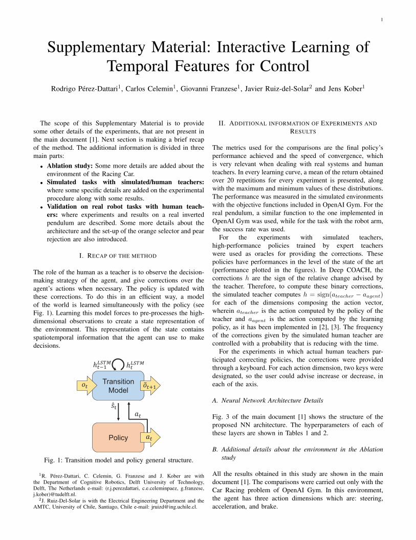
The role of the human as a teacher is to observe the decision-making strategy of the agent, and give corrections over theagent’s actions when necessary. The policy is updated withthese corrections. To do this in an efficient way, a modelof the world is learned simultaneously with the policy (seeFig. 1). Learning this model forces to pre-processes the high-dimensional observations to create a state representation ofthe environment. This representation of the state containsspatiotemporal information that the agent can use to makedecisions.

Policy

Transition

Model !"#$

!"

%"

%"

&'(

)"*$+,-.

)"+,-.

Fig. 1: Transition model and policy general structure.

1R. Pérez-Dattari, C. Celemin, G. Franzese and J. Kober are withthe Department of Cognitive Robotics, Delft University of Technology,Delft, The Netherlands e-mail: (r.j.perezdattari, c.e.celeminpaez, g.franzese,j.kober)@tudelft.nl.

2J. Ruiz-Del-Solar is with the Electrical Engineering Department and theAMTC, University of Chile, Santiago, Chile e-mail: jruizd@ing.uchile.cl.

II. ADDITIONAL INFORMATION OF EXPERIMENTS ANDRESULTS

The metrics used for the comparisons are the final policy’sperformance achieved and the speed of convergence, whichis very relevant when dealing with real systems and humanteachers. In every learning curve, a mean of the return obtainedover 20 repetitions for every experiment is presented, alongwith the maximum and minimum values of these distributions.The performance was measured in the simulated environmentswith the objective functions included in OpenAI Gym. For thereal pendulum, a similar function to the one implemented inOpenAI Gym was used, while for the task with the robot arm,the success rate was used.

For the experiments with simulated teachers,high-performance policies trained by expert teacherswere used as oracles for providing the corrections. Thesepolicies have performances in the level of the state of the art(performance plotted in the figures). In Deep COACH, thecorrections h are the sign of the relative change advised bythe teacher. Therefore, to compute these binary corrections,the simulated teacher computes h = sign(ateacher − aagent)for each of the dimensions composing the action vector,wherein ateacher is the action computed by the policy of theteacher and aagent is the action computed by the learningpolicy, as it has been implemented in [2], [3]. The frequencyof the corrections given by the simulated human teacher arecontrolled with a probability that is reducing with the time.

For the experiments in which actual human teachers par-ticipated correcting policies, the corrections were providedthrough a keyboard. For each action dimension, two keys weredesignated, so the user could advise increase or decrease, ineach of the axis.

A. Neural Network Architecture Details

Fig. 3 of the main document [1] shows the structure of theproposed NN architecture. The hyperparameters of each ofthese layers are shown in Tables 1 and 2.

B. Additional details about the environment in the Ablationstudy

All the results obtained in this study are shown in the maindocument [1]. The comparisons were carried out only with theCar Racing problem of OpenAI Gym. In this environment,the agent has three action dimensions which are: steering,acceleration, and brake.

2

Layer Activation Filters Filter size StrideC1 ReLU 16 3× 3 2C2 ReLU 8 3× 3 2C3 sigmoid 4 3× 3 2DC1 ReLU 8 3× 3 2DC2 ReLU 16 3× 3 2DC3 sigmoid 1 3× 3 2

TABLE I: Hyperparameters of convolutional and deconvolu-tional layers.

Layer Activation N◦ neuronsFC1 tanh 256FC2 tanh 256FC3 tanh 1000FC4 tanh 256FC5 ReLU 1000FC6 ReLU 1000FC7 tanh Task action dimensionR1 LSTM activations hLSTM = 150

TABLE II: Hyperparameters of fully connected and recurrentlayers.

As mentioned in the main document [1], the bottom halfof the frame is occluded in order to force the agent totake decisions based in past observations. An example of theoccluded frame is shown in Fig. 2, the current position of thecar in the road is not observed by the learning policy; however,the entire frame is observed by the policy used as simulatedteacher. Therefore, the corrections are based on appropriateactions with respect to the real state of the environment.

(a) Original frame (b) Occluded frame

Fig. 2: Original frame of the Car Racing environment, on theleft. Occluded frame used as observation in the network, onthe right.

C. Simulated tasks with simulated teachers

The Mountain Car and the Swing-Up Pendulum environmentsoriginally provide, at each time step, their low-dimensionalexplicit state. These are the position and velocity of the car inthe x axis, and the angle and angular velocity of the pendulum,respectively. In order to obtain a high-dimensional observation(raw image) we have modified the source code, such thatthe environment returns an array with the RGB frame thatis rendered.

0 250 500 750 1000 1250 1500 1750Time step

0

20

40

60

80

100

Return

Mountain Car Learning Curve

Teacher

Random policy

D-COACH

DAgger

HG-DAgger

0 0.5 1 1.5 2Time (min)

Fig. 3: D-COACH and DAgger comparison in the MountainCar problem using a simulated teacher.

Mountain Car

The action of the agent is the force applied in order to movethe Car. It is known that the optimal solution for this task isa bang-bang controller (using the extreme actions -1 or 1).Therefore, the correct actions given by the oracle are verydifferent from the initial policy in the whole state space. Thismakes it easier to perform abrupt changes when updating thepolicy for DAgger-like agents than for Deep COACH, becausethe latter performs smaller steps based on incremental andrelative corrections (corrections are in the direction of theoracle’s action, but not directly the actual action).

As it can be seen in Fig. 3, as expected, the learningconvergence is faster for DAgger, followed by HG-DAgger,whereas Deep COACH is the slowest. DAgger converges fasterthan its modified version, HG-DAgger, because the formertrains the policy with corrections provided by the oracle duringevery time step, which is most of the times not feasiblewhen teaching with human users. All agents reach the oracle’sperformance at the end of the learning process.

D. Simulated tasks with human teachers

The validation was executed with 8 participants between 20and 30 years. In the experiments, the users observed thedesired performance of the agent, they received instructionson how to interact with each kind of agent, and they had thechance to practice with the learning agent before recordingresults, in order to get used to the role of teacher. The usersinteract with the learning agent using a keyboard. Users correctthe policies until they consider they cannot improve themanymore, or until a maximum duration of the training sessionof 500 seconds (8.33 minutes). The episodes of the tasks hada duration of 20 seconds, which for Mountain Car means themaximum duration, if the goal is not reached, whereas for thependulum this is constant. The duration of the time steps is0.05 s.

3

0 250 500 750 1000 1250 1500 1750 2000Time step

−25

0

25

50

75

100

Return

Mountain Car Learning Curve w/ Human Teachers

Human

Random policy

D-COACH

HG-DAgger

0 1 2Time (min)

Fig. 4: Mountain Car learning curve with human teachers

Mountain Car

This task is very simple, since users understand properly howto tele-operate the agent, therefore, we could state that for thistask, the teachers are always experts.

Results in Fig. 4 are similar to the ones observed in Fig. 3 inSection II-C, wherein at the beginning HG-DAgger improvesway faster. However, in this case HG-DAgger gets stuck andis outperformed by Deep COACH after 20 seconds. Thishappens as, despite the fact that the teachers are consideredexperts, they could sometimes provide mistaken or ambiguouscorrections. These inconsistencies remain permanently in thedatabase, so it is hard for the user to fix the generated error.

E. Validation on physical systems with human teachers

1) Real Swing-Up Pendulum

This system is similar to the one used previously from OpenAIGym, although in this set-up the dynamics are even muchfaster, and the actions are voltages instead of torques. In thisenvironment a camera is set in front of the pendulum to obtainobservations similar to the simulated environment, as it isshown in Fig. 6, wherein the camera is in the bottom, alignedwith the pendulum. The observation was down-sampled to 32× 32 pixels images, while for all the other tasks the down-sampling was to 64 × 64 pixels. An example of the actualobservation of the camera is in Fig. 7, where it is possible tosee the input of the NN (down sampled image), along with theprediction of the observation in t + 1, with a model that hasbeen trained with the proposed architecture. In this example,it is interesting to observe that the pendulum was rotatingclockwise, therefore the prediction shows the weight of thependulum in a lower position.

Fig. 5 shows the learning curve of 10 runs. In average,the users manage to teach a policy able to balance after29 episodes, and they keep on improving the policy duringthe subsequent episodes. Preliminary tests showed that thesampling time needs to be reduced to 0.025 s to be able tocontrol the system.

0 5000 10000 15000 20000 25000Time step

−1000

−800

−600

−400

−200

0

Return

Real Swing-Up Pendulum Learning Curve

D-COACH

0 1 2 3 4 5 6 7 8 9 10 11Time (min)

Fig. 5: Real Swing-Up Pendulum learning curve.

Fig. 6: Real Swing-Up Pendulum Setup. 1) Pendulum; 2) RGBcamera.

2) Orange selector with a robot arm

As mentioned in the main document [1], this problem iscomposed by two sub-tasks, that are sequentially trained. Inthe experiments, at the beginning when learning the Orangeselection, the teachers corrected the policy only in order tomake the robot to move the end-effector over the horizontalplane. Therefore, the transition model along with a controllerin charge of intercepting the oranges with the end-effector arelearned in the first stage. Then, in order to learn the secondsub-task (Pear rejection) composing the problem, the alreadylearned transition model is reused in the training process of asecond controller that either moves the end-effector close tothe belt or far when a pear is detected. These two controllerswork in parallel since their actions are over different joints.

In the associated video it is shown examples of the actualimages that go to the input of the network, along with theprediction of the next observation. However due to the velocityof the video it is not easy to see that the predicted orangesare slightly shifted. In Fig. 8 are shown examples of threedifferent oranges crossing the field of view of the camera.

4

(a) Network input (b) Observation prediction

Fig. 7: Downsampled observation of the camera, which is theinput of the Network, on the left. Next observation prediction,on the right.

(a) Network input

(b) Observation prediction

Fig. 8: Examples of images in the input of the Network, onthe top. Observation predicted for the next time step by thelearned transition model, on the bottom.

The examples are input-output pairs of the transition model.The oranges moved by the belt are observed by the camerawhile crossing from the top to the bottom of the field of view.It could be seen that the predicted oranges are in a lowerposition with respect to the position observed in the input, i.e.the model learns to predict the movement of the belt.

REFERENCES

[1] R. Pérez-Dattari, C. Celemin, G. Franzese, J. Ruiz-del Solar, and J. Kober,“Interactive learning of temporal features for control,” Robotics andAutomation Magazine (RAM), 2020.

[2] R. Pérez-Dattari, C. Celemin, J. Ruiz-del Solar, and J. Kober, “Contin-uous control for high-dimensional state spaces: An interactive learningapproach,” in 2019 International Conference on Robotics and Automation(ICRA). IEEE, 2019, pp. 7611–7617.

[3] C. Celemin and J. Ruiz-del Solar, “An interactive framework for learningcontinuous actions policies based on corrective feedback,” Journal ofIntelligent & Robotic Systems, pp. 1–21, 2018.