Informative Spectro-Temporal Bottleneck Features for Noise-Robust Speech Recognition

Shuo-Yiin Chang 1,2, Nelson Morgan1, 2

1 EECS Department, University of California-Berkeley, Berkeley, CA, USA 2 International Computer Science Institute, Berkeley, CA, USA

shuoyiin@eecs.berkeley.edu, morgan@icsi.berkeley.edu

Abstract Spectro-temporal Gabor features based on auditory knowledge have improved word accuracy for automatic speech recognition in the presence of noise. In previous work, we generated robust spectro-temporal features that incorporated the power normalized cepstral coefficient (PNCC) algorithm. The corresponding power normalized spectrum (PNS) is then processed by many Gabor filters, yielding a high dimensional feature vector. In tandem processing, an MLP with one hidden layer is often employed to learn discriminative transformations from front end features, in this case Gabor filtered power spectra, to probabilistic features, which are referred as PNS-Gabor MLP. Here we improve PNS-Gabor MLP in two ways. First, we select informative Gabor features using sparse principle component analysis (sparse PCA) before tandem processing. Second, we use a deep neural network (DNN) with bottleneck structure. Experiments show that the high-dimensional Gabor features are redundant. In our experiment, sparse principal component analysis suggests Gabor filters with longer time scales are particularly informative. The best of our experimental modifications gave an error rate reduction of 15.5% relative to PNS-Gabor MLP plus MFCC, and 41.4% better than an MFCC baseline on a large vocabulary continuous speech recognition task using noisy data.

Index Terms: LVCSR, spectro-temporal feature, robust speech recognition, deep neural network, sparse principal component analysis

1. Introduction and Previous work When they are paying attention, humans speech recognition is far better than our automatic systems, particularly in the presence of noise. This often inspires researchers to seek more robust features based on auditory models. In the past decade, physiological experiments on different mammalian species have revealed that the neurons in the primary auditory cortex are sensitive to particular spectro-temporal patterns referred to as spectro-temporal receptive fields (STRFs) [1]. Based on these experimental results, spectro-temporal features, which serve as a model for STRFs, have been applied to ASR. Several studies have successfully incorporated Gabor function approximations into ASR [2][3][4]. In general, these approaches define a series of spectral, temporal, and spectral-temporal modulation filters which can be seen as roughly modeling neuron firing patterns for particular spectro-temporal signal components, but in any case they provide a large range of transformations of the time-frequency plane. Purely temporal features such as TRAPS [5] and HATS [6] can be regarded as special cases of spectro-temporal features. Spectro-temporal features have been successfully used for

recognition of both clean and noisy speech, which provides a different solution to most existing robsutness methods focusing on compensating the difference of clean and noisy speech in the models [7][8] or the features [9][10][11]. In [12], a more robust spectro-temporal representation incorportating key parts of the power normalized cepstral coeffieients (PNCCs) algorithm [10] was employed. We referred to this feature set as power-normalized spectrum Gabor (PNS-Gabor).

However, due to the use of a large number of Gabor filters, the feature dimension is quite high, and it is likely that many of the features are redundant. Tsai and Morgan [13,14] showed that a small number of filters dominated the performance for the speech activity detection task. In this paper, we employ sparse PCA [15][16] as a feature selection tool to find informative Gabor features, which maximize data variance. Sparse PCA extended classical PCA by maximizing data variance using sparse principal vectors. The property makes it easy to interpret and also is useful for feature selection to discard uninformative components.

In tandem processing, an MLP with single hidden layer is commonly employed to transform front end values (e.g., the Gabor filtered time-frequency plane) to probabilistic features [17]. An MLP with a bottleneck layer is also commonly used [18][19]. However, it is difficult benefit from increasing the number of hidden layers without using some kind of initialization, particularly because the layers far from the target are little changed by the usual stochastic gradient learning algorothms. Hinton et al [20] proposed an unsupervised training algorithm based on restricted Boltzman machine (RBM) moving the parameters to a good initial. Pre-trained deep neural networks have been used to decrease WER [21][22]. Here, we exploit pre-trained deep neural network using Gabor input to improve robustness for recognition of noisy speech.

Comparison of the proposed method and the previous PNS-Gabor MLP(3l) [12] is shown in Fig. 1.

Figure 1 Comparison of proposed method (top path) and our previous work (bottom path).

Sparse principle

component analysis

Bottleneck Deep Neural

Network

Informative PNSGb� BN DNN

Gabor filters

Power normalized spectrum

Gabor filters

Conventional 3-layers MLP

PNSGb-MLP(3l)

2. Proposed Method

2.1. PNS Gabor features

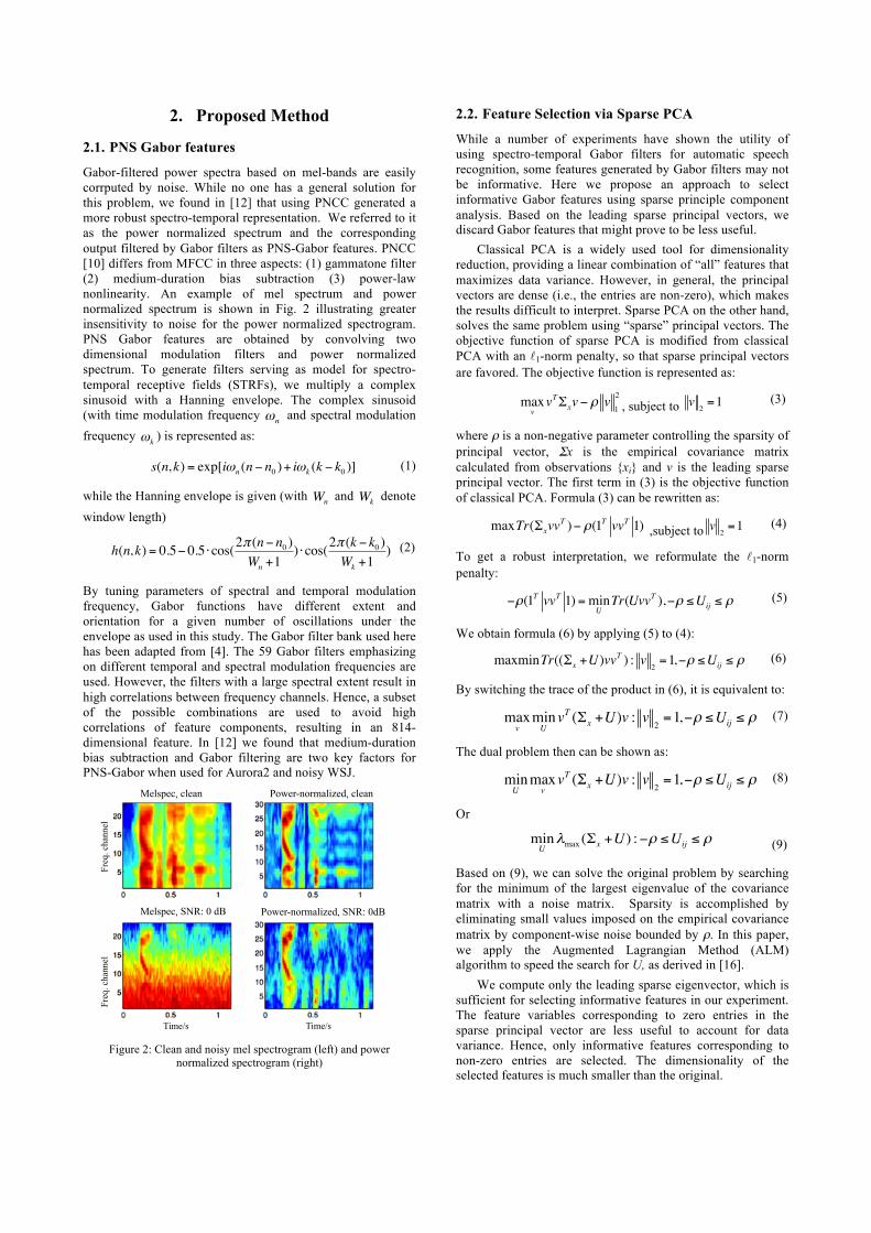
Gabor-filtered power spectra based on mel-bands are easily corrputed by noise. While no one has a general solution for this problem, we found in [12] that using PNCC generated a more robust spectro-temporal representation. We referred to it as the power normalized spectrum and the corresponding output filtered by Gabor filters as PNS-Gabor features. PNCC [10] differs from MFCC in three aspects: (1) gammatone filter (2) medium-duration bias subtraction (3) power-law nonlinearity. An example of mel spectrum and power normalized spectrum is shown in Fig. 2 illustrating greater insensitivity to noise for the power normalized spectrogram. PNS Gabor features are obtained by convolving two dimensional modulation filters and power normalized spectrum. To generate filters serving as model for spectro-temporal receptive fields (STRFs), we multiply a complex sinusoid with a Hanning envelope. The complex sinusoid (with time modulation frequency and spectral modulation frequency ) is represented as:

(1)

while the Hanning envelope is given (with and denote window length)

(2)

By tuning parameters of spectral and temporal modulation frequency, Gabor functions have different extent and orientation for a given number of oscillations under the envelope as used in this study. The Gabor filter bank used here has been adapted from [4]. The 59 Gabor filters emphasizing on different temporal and spectral modulation frequencies are used. However, the filters with a large spectral extent result in high correlations between frequency channels. Hence, a subset of the possible combinations are used to avoid high correlations of feature components, resulting in an 814-dimensional feature. In [12] we found that medium-duration bias subtraction and Gabor filtering are two key factors for PNS-Gabor when used for Aurora2 and noisy WSJ.

Figure 2: Clean and noisy mel spectrogram (left) and power

normalized spectrogram (right)

2.2. Feature Selection via Sparse PCA

While a number of experiments have shown the utility of using spectro-temporal Gabor filters for automatic speech recognition, some features generated by Gabor filters may not be informative. Here we propose an approach to select informative Gabor features using sparse principle component analysis. Based on the leading sparse principal vectors, we discard Gabor features that might prove to be less useful.

Classical PCA is a widely used tool for dimensionality reduction, providing a linear combination of “all” features that maximizes data variance. However, in general, the principal vectors are dense (i.e., the entries are non-zero), which makes the results difficult to interpret. Sparse PCA on the other hand, solves the same problem using “sparse” principal vectors. The objective function of sparse PCA is modified from classical PCA with an 1-norm penalty, so that sparse principal vectors are favored. The objective function is represented as:

, subject to (3)

where ρ is a non-negative parameter controlling the sparsity of principal vector, Σx is the empirical covariance matrix calculated from observations {xi} and v is the leading sparse principal vector. The first term in (3) is the objective function of classical PCA. Formula (3) can be rewritten as:

maxTr(ΣxvvT )− ρ(1T vvT 1) ,subject to

(4)

To get a robust interpretation, we reformulate the 1-norm penalty:

−ρ(1T vvT 1) =minUTr(UvvT ),−ρ ≤Uij ≤ ρ (5)

We obtain formula (6) by applying (5) to (4):

maxminTr((Σx +U)vvT ) : v

2=1,−ρ ≤Uij ≤ ρ (6)

By switching the trace of the product in (6), it is equivalent to:

(7)

The dual problem then can be shown as:

(8)

Or

(9)

Based on (9), we can solve the original problem by searching for the minimum of the largest eigenvalue of the covariance matrix with a noise matrix. Sparsity is accomplished by eliminating small values imposed on the empirical covariance matrix by component-wise noise bounded by ρ. In this paper, we apply the Augmented Lagrangian Method (ALM) algorithm to speed the search for U, as derived in [16].

We compute only the leading sparse eigenvector, which is sufficient for selecting informative features in our experiment. The feature variables corresponding to zero entries in the sparse principal vector are less useful to account for data variance. Hence, only informative features corresponding to non-zero entries are selected. The dimensionality of the selected features is much smaller than the original.

ωn

ωk

s(n,k) = exp[iωn (n− n0 )+ iωk (k − k0 )]

Wn Wk

h(n,k) = 0.5− 0.5 ⋅cos(2π (n− n0 )Wn +1

) ⋅cos(2π (k − k0 )Wk +1

)

Melspec��clean Power-normalized��clean

Melspec��SNR: 0 dB Power-normalized��SNR: 0dB

Freq

. cha

nnel

Fr

eq. c

hann

el

Time/s Time/s

maxvvTΣxv− ρ v

1

2 v2=1

v2=1

maxvminUvT (Σx +U)v : v 2

=1,−ρ ≤Uij ≤ ρ

minUmax

vvT (Σx +U)v : v 2

=1,−ρ ≤Uij ≤ ρ

minUλmax (Σx +U) :−ρ ≤Uij ≤ ρ

2.3. Bottleneck features using Pre-trained Deep Neural Network

A bottleneck feature vector commonly is generated by a narrow-dimensional layer in the middle of a five-layer MLP. While using even more layers can improve the network, better initialization can be a significant help when using more layers. Restricted Boltzman machine (RBM) pre-training [22], which is unsupervised, is one method that has been introduced to initialize the parameters of neural network. For completeness, we briefly remind the reader of the main idea here.

RBM is a bipartite graph modeling the joint distribution of a layer of stochastic visible units and hidden units. Only visible-hidden connections are allowed. For Bernoulli-Bernoulli RBM, the joint distribution is defined as:

(10)

where Z is the normalization term, E(v,h) is energy function. b and c are the bias for visible layer v and hidden layer h while W is a symmetric weight matrix between v and h. Based on (10), the posterior of hidden units can be obtained as:

(11)

Formula (11) is essentially the forward propagation procedure of neural network. Hence, RBM can be applied to model each pair of layers of a neural network. The input layer usually consists of real-valued variables, so a Gaussian-Bernoulli RBM is employed. The energy function for this is revised as:

(12)

while (11) still holds. The parameters of the MLP, therefore, get good initialization by maximizing the log likelihood of the RBM. Training of RBM can be found in [21].

3. Experimental Setup The proposed approach was evaluated using “re-noised” Wall Street Journal (WSJ) speech and far-field meeting corpus. For WSJ, we started out with clean data taken from 77.8 hours of the WSJ1 dataset (284 speakers) for training and 0.8 hours of the WSJ-eval94 dataset (20 speakers) for testing. Estimated additive and channel noise from degraded recordings was applied to both training and testing dataset using “renoiser” tool [23]. Designed for use in the DARPA RATS project, the system analyzes data from RATS rebroadcast example signals (in this case, LDC2011E20) to estimate the noise characteristic including SNRs and frequency-shifts; the original data is described in [24] and consists of a variety of continuous speech sources that have been transmitted and received over 8 different radio channels, resulting in significant signal degradations. The 8 radio channel characteristics were specified in [12]. We applied the same noise characteristics to WSJ data and it is referred as “re-noised WSJ”. The results reported here are WERs averaging over clean and 8 noisy channels. For the far-field part of the meeting data, we used a single distant microphone channel from a dataset of spontaneous meeting speech recorded at ICSI [25]. Our training set was based on the meeting data used for adaptation in the SRI-ICSI meeting recognition system [26]. For the test set we used the ICSI meetings drawn from the NIST RT eval sets [27]. The resulting training set was 20 hours long (26

speakers) and the testing set was 1 hour of data (18 speakers). We used the HTK toolkit [28] for both training and decoding with both databases. The acoustic models were cross-word triphones estimated with maximum likelihood. For re-noised WSJ, the resulting triphone states were clustered to 5000 tied states, each of which was modeled by 32-component of Gaussian mixture model. We used version 0.6 of the CMU pronunciation dictionary and the standard 5k bigram language model created at Lincoln Labs for the 1992 evaluation. For the single distant microphone (SDM) portion of the far-field meeting corpus, 2500 states were modeled by Gaussian mixture models with 8 components per state. The 10k tri-gram SRI LM [29] was trained by interpolating Switchboard, meetings, Fisher, Hub4-LM96, and TDT4. To be compatible with the SRI LM, we used the SRI pronunciation dictionary.

All the networks were trained with a temporal context window of 9 successive frames. The output layer consisted of 41 context-independent phonetic targets. We used a learning rate of .002 in the RBM pre-training step. For back propagation following the pre-training, we began with a learning rate of .008 and reduced the learning rate by factors of two once cross-validation indicated limited progress with each learning rate, and continued until cross-validation showed essentially no further progress. We took the logarithm of the posterior probability features generated from the output of the MLP, and reduced the dimensionality via PCA to 25. For bottleneck features, the size of the bottleneck layer was set to 25. In both cases, MFCCs were concatenated with the MLP-based features, resulting in a 64-dimensional feature vector. Means and variances were normalized per utterance before HMM training and testing for all the features in this paper.

4. Results and Discussion We first compared different configurations of neural network using 814 dimensional PNS-Gabor inputs with 9 frames, or 7326 inputs. Next, feature selection using sparse PCA was studied. Finally, we compared the result with state-of-the-art features and showed that the informative feature selection is fairly invariant to differences between the two corpora used.

In Fig 3, we show results for several different configurations of neural network using PNS-Gabor input on re-noised WSJ: a three-layer MLP, a four-layer deep neural network (DNN), a five-layer bottleneck DNN and a six-layer bottleneck DNN. The 3-layer MLP used one large hidden layer. For the 4-layer DNN, two 500 unit hidden layers were used to model phone classes. In the 5-layer DNN, these 2 hidden layers were separated by the small (25) bottleneck layer. The 6-layer bottleneck configuration included an additional 500-unit layer after the first hidden layer, so that the initial transformations are similar to those of the 4-layer

Figure 3: Re-noised WSJ WERs of 814-d PNS-Gabor input using four different neural network architectures

P(v,h) = e−E (v,h)

Z,E(v,h) = −bTv− cTh− vTWh

P(hi =1| v) = sigmoid(ci + vTWi )

E(v,h) = 12(v− b)T (v− b)− cTh− vTWh

7326:500:41

29

30

31

32

33

34

35

3-layer 4-layer 5-layer, BN 6-layer, BN

Random initialization RBM pre-training

7326:500:500:41 7326:500:25:500:41 7326:500:500:25:500:41

WER

network, followed then by the bottleneck portion. The number of parameters remained quite similar, ranging from 3.7M to 3.9M. The specific configurations are described in Fig. 3.

As shown in Fig 3, the 4-layer DNN and the 6-layer bottleneck DNN performed significantly better. Comparing the 6-layer bottleneck DNN to the 4-layer DNN, bottleneck compression slightly decreases WER. Another observation is that RBM always helps when training deep neural networks, as has been observed by many others. The 6-layer bottleneck DNN with RBM pre-training was best in our experiments, so we used this architecture for the rest of the work reported here.

In Table 1, we compare 814 dimensional PNS-Gabor features and the dimensionally reduced “informative” PNS-Gabor feature selected via sparse PCA. In this experiment, ρ was set to .008, resulting in 271 dimensional features. The size of hidden layers was increased to 1000 so that total number of parameters was comparable for the comparison. As shown in Table 1, the sparse-PCA selection was 6.7% relative better than using all of the features. Aside from this improvement, the approach also made feature generation more efficient. The sparse PCA approach was furthered compared with classical PCA. Results also suggest that using the reduced “informative” features is better than using the linear combination of all features obtained by classical PCA.

Using the sparse principal vector, we observed the suggested importance of Gabor filters in Fig. 4. The darker areas represent the degree of importance (at least in terms of variance) based on how many channels generated by the filter were selected. As shown in Fig 4, filters with low temporal modulation frequency appear to be useful for maximizing data variance. The features emphasizing on temporal modulation frequency of 0, 2,4 and 3.9 Hz account for 94.1% of the weights of the leading sparse principal vector. The corresponding filter lengths are roughly 1, 0.7 and 0.5 sec. It suggests that Gabor filters with longer time scales are particularly informative for ASR, at least for these tests.

In Table 2, we compared the proposed feature with MFCC baseline and state-of-the-art features: the so-called “advanced frond end” (AFE) [10] and PNCC [11] (For the matched clean training-testing condition, WER for MFCC was 6.7%, but here we focus on the multi-conditional training task). Our previous feature set [12] was shown in column (4). A six-layer bottleneck DNN was employed in column (5) while informative selection was further applied in column (6). Overall, the proposed feature in (6) is 15.5% better than PNS-Gabor MLP(3l) plus MFCC and 41.4% relative better than the MFCC baseline.

In Table 3, we evaluated the proposed feature on the far-field meeting test. The proposed feature is presented in (5) and (6). In column (5), sparse PCA was trained on re-noised WSJ. In contrast, we trained sparse PCA on meeting data in column (6). The difference between (5) and (6) is tiny, which suggests that the proposed feature selection approach is invariant to different corpora. The proposed feature reduces the WER by 14% relative to MFCC on the meeting test set.

Table 1: Informative and original PNS-Gabor input for re-noised WSJ

Figure 4: Importance of Gabor filters based on sparse PCA

5. Conclusions Here we report our use of sparse PCA, informative PNS-Gabor features, and bottleneck deep neural networks using two large hidden layers following the input layer. The key factor distinguishing the proposed feature set from our earlier work is discarding uninformative shorter features. Non-linear dimension reduction from the bottleneck feature also gave slight improvement. Overall, the proposed feature is 15.5% relative better than previous PNS-Gabor MLP(3l) plus MFCC and 41.4% relative better than MFCC on re-noised WSJ. For far-field meeting corpus, we can reduce word error rate by 14% relative to MFCC.

6. Acknowledgements We thank Bernd Meyer, Dan Ellis for help in setting up the feature extraction and re-noised WSJ data. We thank to Chanwoo Kim and Richard Stern for use of PNCC. This material is based on work supported by the Defense Advanced Research Projects Agency (DARPA) under Contract No. D10PC20024. Any opinions, findings, and conclusions or recommendations expressed in this material are those of the author(s) and do not necessarily reflect the view of the DARPA or its Contracting Agent, the U.S. Department of the Interior, National Business Center, Acquisition & Property Management Division, Southwest Branch.

Table 2: Re-noised WSJ WERs for state-of-the-art feature

Table 3: WERs for far-field meeting corpus

6-layer BN DNN Input Dim. WER PNS-Gabor 814 31.02

PNS-Gabor, classical PCA 271 29.57 Informative PNS-Gabor 271 28.93

!

75%~100% channels selected

50%~75% channels selected

25%~50% channels selected

0%~25% channels selected

Temporal modulation frequency /Hz Spec

tral m

odul

atio

n fr

eque

ncy

/ [cy

cl./c

hann

el]

WER

(1) MFCC

(2) ETSI-AFE

(3) PNCC

(4) PNSGb-MLP(3l)

+MFCC

(5) PNSGb-BN DNN

+MFCC

(6) Inf.

PNSGb-BN DNN +MFCC

Clean 19.06 19.22 16.21 14.04 14.34 12.70 Channel A 42.22 36.89 32.60 26.78 24.09 22.24 Channel B 49.25 48.44 46.79 35.09 31.67 29.05 Channel C 51.05 49.38 47.15 34.79 30.72 28.88 Channel D 59.52 54.49 58.18 40.35 36.29 33.65 Channel E 78.43 74.05 72.93 55.46 50.43 47.87 Channel F 65.58 62.48 60.41 44.28 40.79 37.96 Channel G 23.55 23.25 20.72 17.24 16.01 15.44 Channel H 56.23 51.56 53.01 39.39 34.8 32.64 Average 49.4 46.6 45.3 34.2 31.0 28.9 !

Feature

(1) MFCC

(2) ETSI-AFE

(3) PNCC

(4) PNSGb- MLP(3l) + MFCC

(5) Inf. PNGb- BN,DNN + MFCC

(6) Inf. PNSGb-

BN,DNN +MFCC

SPCA training

set - - - no re-noised

WSJ meeting corpus

WER 64.3 63.8 63.2 58.8 55.4 55.5

!

7. References [1] N. Mesgarani, and S. Shamma, “Speech Processing with a

Cortical Representation of Audio”, Proc. ICASSP 2011, May 2011, pp. 5872-5875.

[2] M. Kleinschmidt, “Localized spectro-temporal features for automatic speech recognition,” in Proc. of Eurospeech, 2003, Sep 2003, pp. 2573–2576.

[3] F. Joublin X. Domont, M.Heckmann and C. Goerick, “Hierarchical spectro-temporal features for robust speech recognition” Proc. ICASSP 2008, March 2008, pp. 4417-4420

[4] Meyer, B. T., Ravuri, S. V., Schadler, M. R., and Morgan, N., “Comparing Different Flavors of Spectro-Temporal Features for ASR”, in Proc. of Interspeech, pp. 1269 - 1272, 2011.

[5] H. Hermansky and S. Sharma, “Temporal patterns (TRAPs) in ASR of noisy speech,” Proc. ICASSP 1999, March 1999, pp. 289-292 vol. 1.

[6] B.Y. Chen, Q. Zhu, and N. Morgan, “A Neural Network for Learning Long-Term Temporal Features for Speech Recognition,” Proc. ICASSP 2005, March 2005, pp. 945-948

[7] O. Kalinli, M.L. Seltzer, and A. Acero, “Noise adaptive training using a vector Taylor series approach for noise robust automatic speech recognition,” in Proc. ICASSP, 2009, pp. 3825-3828

[8] F. Flego and M. J. F. Gales, “Factor Analysis Based VTS Discriminative Adaptive Training” Proc. ICASSP. IEEE, 2012, pp. 4669–4672.

[9] H. Franco, M. Graciarena, and A. Mandal, “Normalized amplitude modulation features for large vocabulary noise-robust speech recognition”, Proc. ICASSP 2012, March 2012, pp. 4117-4120

[10] C. Kim and R. M. Stern, “Feature extraction for robust speech recognition based on maximizing the sharpness of the power distribution and on power flooring”, in Proc. ICASSP, pp. 4574–4577, 2010.

[11] Speech Processing, Transmission and Quality Aspects (STQ); Distributed Speech Recognition; Adv. Front-end Feature Extraction Algorithm; Compression Algorithms, ETSI ES 202 050 Ver. 1.1.5, 2007

[12] S.Y. Chang, B. Meyer and N. Morgan “Spectro-temporal features for noise-robust speech recognition using power-law nonlinearity and power-bias subtraction”, Proc. ICASSP 2013

[13] T. J. Tsai and N. Morgan “ Longer Features: They Do a Speech Detector Good” Proc. Interspeech 2012

[14] T. J. Tsai and N. Morgan “ Speech activity detection: an economics approach” Proc. ICASSP 2013

[15] A. d’Aspremont, L. Ghaoui, M. I. Jordan, and G. R. G. Lanckriet. “A direct formulation for sparse PCA using semidefinite programming. SIAM Review, Vol. 49, No. 3. (July 2007), pp. 434-448

[16] N. Naikal, A. Yang, and S. Sastry “Informative feature selection for object recognition via sparse PCA”. In Proceedings of the 13th International Conference on Computer Vision (ICCV), 2011, pp. 818-825

[17] H. Hermansky, D. Ellis, and S. Sharma, “Tandem connectionist feature extraction for conventional HMM systems”, Proc. ICASSP, Istanbul, Turkey, 2000, June 2000, pp. 1635-1638 vol.3.

[18] F. Grezl, M. Karafiat and S. Kontar and J. Cernocky, “Probabilistic and bottle-neck features for LVCSR of meetings” Proc. ICASSP 2007, pp. 757-760

[19] F. Grezl and P. Fousek, “Optimizing bottle-neck features for LVCSR”, Proc. ICASSP 2008, pp. 4729-4732

[20] G. Hinton and R. Salakhutdinov, “Reducing the dimensionality of data with neural networks,” Science, vol. 313, no. 5786, pp. 504 – 507, 2006

[21] G.E. Dahl, D. Yu, L. Deng, and A. Acero, "Context Dependent Pretrained Deep Neural Networks for Large Vocabulary Speech Recognition", IEEE Trans. Audio, Speech, and Lang. Proc. - Special Issue on Deep Learning for Speech and Lang. Proc., 2011

[22] D. Yu and M. Seltzer “Improved Bottleneck Features Using Pretrained Deep Neural Networks” in Proc. Interspeech 2011

[23] “Renoiser web page,” http://labrosa.ee.columbia.edu/projects/renoiser/create_wsj.html

[24] K.Walker and S. Strassel, “The rats radio traffic collection system,” in Proc. of ISCA Odyssey, 2012.

[25] A. Janin, D. Baron, J. Edwards, D. Ellis, D. Gelbart, N. Morgan, B. Peskin, T. Pfau, E. Shriberg, A. Stolcke, and C. Wooters, “The ICSI meeting corpus,” in Proceedings of International Conference on Acoustics, Speech, and Signal Processing, 2003

[26] A. Stolcke, X. Anguera, K. Boakye, O. Cetin, A. Janin, M. Magimai-Doss, C. Wooters, and J. Zheng, “The SRI-ICSI Spring 2007 Meeting and Lecture Recognition System,” in Proceedings of the Second International Workshop on Classification of Events, Activities, and Relationships (CLEAR 2007) and the Fifth Rich Transcription 2007 Meeting Recognition (RT 2007), 2007.

[27] “Rt-2002 evaluation plan web page,” http://www.itl.nist.gov/iad/mig/tests/rt/2002/docs/rt02 eval plan v3.pdf.

[28] S. Young, D. Kershaw, J. Odell, D. Ollason, V. Valtchev, and P. Woodland. The HTK Book. Cambridge,United Kingdom: Entropic Ltd.

[29] O. Cetin and A. Stolcke, “Language modeling in the ICSI-SRI Spring 2005 meeting speech recognition evaluation system,” Tech. Rep., International Computer Science Institute, 2005.