HAL Id: hal-00592960https://hal.archives-ouvertes.fr/hal-00592960

Submitted on 3 May 2011

HAL is a multi-disciplinary open accessarchive for the deposit and dissemination of sci-entific research documents, whether they are pub-lished or not. The documents may come fromteaching and research institutions in France orabroad, or from public or private research centers.

L’archive ouverte pluridisciplinaire HAL, estdestinée au dépôt et à la diffusion de documentsscientifiques de niveau recherche, publiés ou non,émanant des établissements d’enseignement et derecherche français ou étrangers, des laboratoirespublics ou privés.

Interaction fluide structure appliquée a l’analyse desvoiles

Daniele Trimarchi, Stephen Turnock, Dominic Taunton, Dominique Chapelle,Marina Vidrascu

To cite this version:Daniele Trimarchi, Stephen Turnock, Dominic Taunton, Dominique Chapelle, Marina Vidrascu. Inter-action fluide structure appliquée a l’analyse des voiles. 10e colloque national en calcul des structures,May 2011, Giens, France. 8 p., 2011. <hal-00592960>

CSMA 201110e Colloque National en Calcul des Structures

9-13 Mai 2011, Presqu’île de Giens (Var)

Fluid Structure Interactions

applied to Downwind Yacht Sails

D. Trimarchi1, M. Vidrascu2, D. Taunton1, S.R. Turnock1,D. Chapelle2

1 Fluid Structure Interactions Research Group, University of Southampton, United Kingdom, daniele.trimarchi@soton.ac.uk2 INRIA, MACS team, France

Abstract — Sail analysis is a rapidly evolving field, since it has a big impact in the performances ofyachts. In the present approach, a weak coupling in Arbitrary Lagrangian Eulerian (ALE) configurationhas been chosen. The flow is analyzed with a Reynolds Averaged Navier Stokes (RANS) Finite Volume(FV) solver with turbulence models, whereas the structural analysis is performed with non-linear MITCShell Finite Elements (FE). The approach and examples are presented and discussed with regards to atwo dimensional downwind sail section in turbulent flow.Keywords — Sail analysis, RANSE, Finite Elements, Fluid Structure Interactions.

1 Introduction

Downwind sail analysis is particularly complex because of the number of phenomena interacting to-gether. From a fluid perspective, sails are thin laminates operating in a wide range of angles of attack.Because of the large angle of attack and the device curvature the force generation results in an interme-diate regime of lift and drag, with large regions of separated flow. Due to the size and the relevant windspeed, transition to turbulent flow arises in the very first part of the device, behind the leading edge. Dueto adverse pressure gradients and the sharp corner leading edge, separation bubbles are likely to form onthe edges of the device, thus further increasing the flow complexity.

Unsteady phenomena can be driven by a composition of fluid unsteadiness such as the vortex shed-ding, and unsteadiness induced by the boat’s motions in seaway or the gusts. The impact of unsteadyflows can be identified in a global increase in the force generation process [12] .

In the approach presented here the flow is simulated with a Finite Volume (FV) approach. TheC++ library OpenFOAM [7] has been chosen, since it includes unsteady RANS solvers and the mostcommonly adopted turbulence models, as well as dynamic mesh handling capabilities.

From a structural point of view sails are constituted by thin orthotropic laminates, which can beassumed to be in large displacements-small strains regime. Since sails are made of fabrics, wrinklingmay appear. This is a buckling related phenomenon, which determines the formation of oscillations andwrinkles onto the fabric surface. Since Wrinkling locally modify stress distributions in the fabric, it mayhave strong influence on the whole deformed equilibrium shape.

Due to its computational cost, only a few authors approached coupled fluid structure interaction(FSI) analysis of downwind sails. In such works, the flow is generally modelled with FV Methodsfor the solution of RANS equations [8], and SST turbulence model [3]. Downwind sail fluid structureinteractions have been presented, where a weak steady coupling is performed between RANS and FEsolvers [9]. From a structural perspective, the sailcloth is usually analyzed with CST membranes [4].Such elements derive from a rather simplified formulation, based on the geometrical observation thata triangle is uniquely defined by the sides length, therefore that the element’s strain can be entirelyevaluated using such measure.

Furthermore, due to the lack of bending stiffness, the membrane model is inadequate to deal withsome particular situations, in particular when wrinkling occurs. Wrinkling being buckling related, itsdevelopment is in fact completely controlled by the bending stiffness. The membrane model resultsin such cases undetermined, and strong singularities may appear and affect the solution. The problemis generally overcome with ad-hoc wrinkling models, the scope of which is to modify the constitutive

1

relationship when a wrinkling criterion is satisfied.In the present approach the sail fabric is simulated with the use of non-linear shells of the Mixed

Interpolation Tensorial Components (MITC) family [2]. Compared to membranes, the shell model in-cludes the bending stiffness, thus all the relevant strain components are represented. This assures thatthe model is never undetermined, thus wrinkling is directly represented without the need of additionalmodels [14, 13]. The MITC shells has been chosen, since this particular model is formulated for avoidingnumerical locking, a phenomenon arising and affecting results in the analysis of thin shells. The struc-tural analysis is carried out with Shelddon, a Fortran Finite Element (FE) package developed by INRIAand allowing the use of non-linear shells MITC.

Fluid structure coupling is performed in an Arbitrary Lagrangian Eulerian (ALE) framework usingthe dynamic mesh capabilities of OpenFOAM. Data are passed between fluid and structure frameworkusing openMPI, already adopted in OpenFOAM for high performance parallel computing purposes.

2 Methods

The fluid analysis is carried out with the FV C++ library OpenFOAM. Two main solvers have beenused for fluid analysis and FSI. In the first case, the pisoFOAM solver has been chosen. This is a semi-implicit uncoupled solver for transient incompressible flows. It is based upon the FV discretization of theNavier-Stokes equations. FSI coupled analysis has been carried out using the PimpleDyMFOAM solver.This solver allows the use of dynamic meshes in ALE framework, thus it makes possible conservativemovements of mesh regions within the fluid domain. The standard solver has been modified by theauthor in order to impose the boundary movement specified by the structural solver, and allow the datacommunication via MPI. In both cases the SST turbulence model has been chosen. This is a blend of κ-εand κ- ω models [6], which is generally considered one of the best compromises for sail type flows [3].

The structural analysis is performed with the Shelddon finite element library [11]. The sail fabric isrepresented by non-linear four nodes MITC shells. An isotropic linear elastic constitutive relationshiphas been chosen, since a small strain regime is assumed. The use of shells rather than membranes has theadvantage that no additional models are required for the treatment of wrinkling, which can be representeddirectly [12]. Severe convergence issues may arise, due to the very limited thickness of the fabric, whichcause the system to be very ill conditioned. This problem has been overcome using a dynamic routinewith Rayleigh Damping, the details of which can be found in [12]. For completeness however, the basicequations are reported below. By discretization with the mid-point rule, the structural dynamic governingequation reads, in a linear framework:

(

4M

δt2 +2C

δt+KT

)

· yn+ 12=

(

4M

δt2 +2C

δt

)

· yn +2M

δt· yn +Fn+ 1

2(1)

where:

M, C, KT are the structure’s mass, damping and tangent stiffness matricesδt is the time-stepyn, yn are the position and velocity vectors at the time-step n yn+ 1

2= (yn+1+yn)

2

Mass and Stiffness matrices definition can be found in [1], whereas Rayleigh definition of dampinghas been chosen. The damping matrix is a linear combination of Mass and Stiffness matrices, wheretuning coefficients c1 and c2 can be opportunely defined for optimal convergence rate. Since the structuraldynamics is determined by arbitrary coefficients, the evolution of the structure follows a pseudo-timestep. The purpose is then to reach a steady equilibrium state for a given load, rather than to represent areal dynamics.

C = c1 ·M+ c2 ·K (2)

The cable holding the sail (sheet) has been simulated by directly expressing the cable strain energy.The terms to be added to the right hand side and the stiffness matrix are then obtained by differentiatingrespectively once and twice with respect to the vector y, which stores the displacement of the constrainednodes. Using the Green-Lagrange strain measure, the the cable potential can be expressed as:

2

Wc =Ec ·Ac

2· [(x0 − x f + y)2 − ((1+ ε)(x0 − x f ))

2]2 (3)

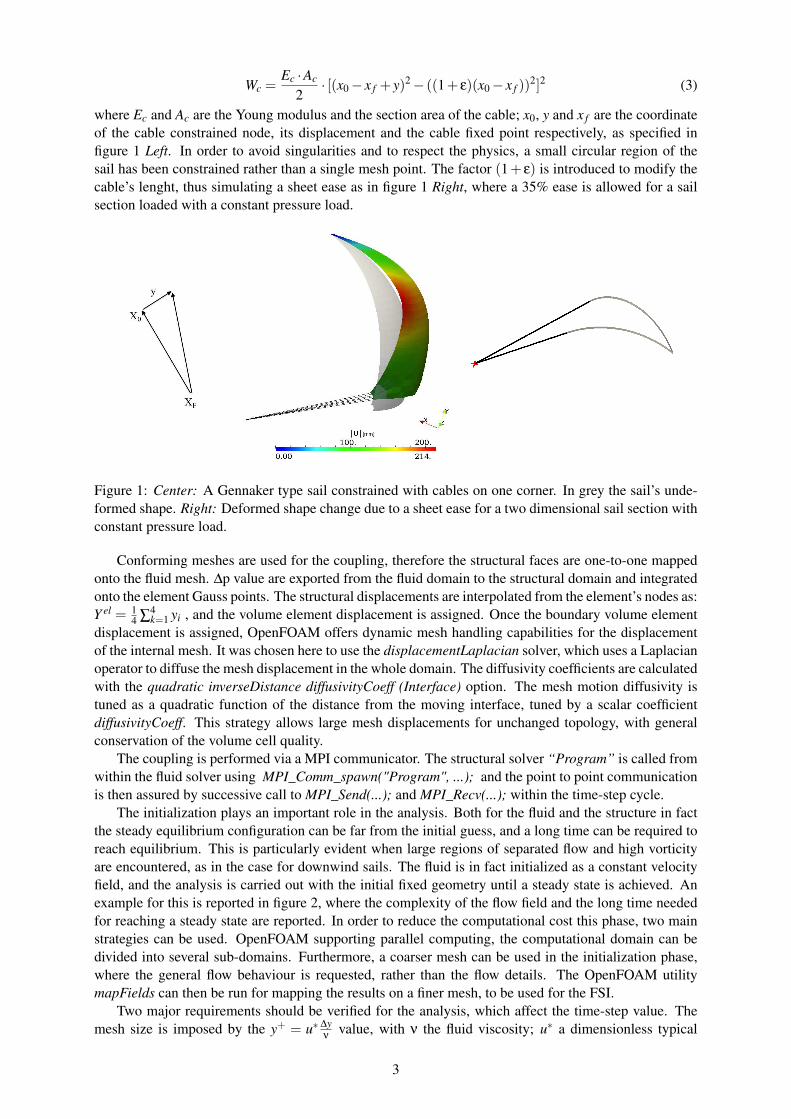
where Ec and Ac are the Young modulus and the section area of the cable; x0, y and x f are the coordinateof the cable constrained node, its displacement and the cable fixed point respectively, as specified infigure 1 Left. In order to avoid singularities and to respect the physics, a small circular region of thesail has been constrained rather than a single mesh point. The factor (1+ ε) is introduced to modify thecable’s lenght, thus simulating a sheet ease as in figure 1 Right, where a 35% ease is allowed for a sailsection loaded with a constant pressure load.

Figure 1: Center: A Gennaker type sail constrained with cables on one corner. In grey the sail’s unde-formed shape. Right: Deformed shape change due to a sheet ease for a two dimensional sail section withconstant pressure load.

Conforming meshes are used for the coupling, therefore the structural faces are one-to-one mappedonto the fluid mesh. ∆p value are exported from the fluid domain to the structural domain and integratedonto the element Gauss points. The structural displacements are interpolated from the element’s nodes as:Y el = 1

4 ∑4k=1 yi , and the volume element displacement is assigned. Once the boundary volume element

displacement is assigned, OpenFOAM offers dynamic mesh handling capabilities for the displacementof the internal mesh. It was chosen here to use the displacementLaplacian solver, which uses a Laplacianoperator to diffuse the mesh displacement in the whole domain. The diffusivity coefficients are calculatedwith the quadratic inverseDistance diffusivityCoeff (Interface) option. The mesh motion diffusivity istuned as a quadratic function of the distance from the moving interface, tuned by a scalar coefficientdiffusivityCoeff. This strategy allows large mesh displacements for unchanged topology, with generalconservation of the volume cell quality.

The coupling is performed via a MPI communicator. The structural solver “Program” is called fromwithin the fluid solver using MPI_Comm_spawn("Program", ...); and the point to point communicationis then assured by successive call to MPI_Send(...); and MPI_Recv(...); within the time-step cycle.

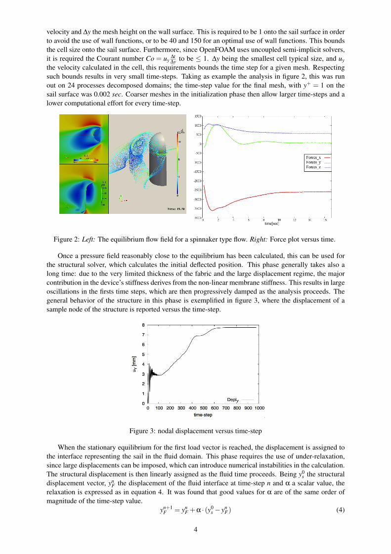
The initialization plays an important role in the analysis. Both for the fluid and the structure in factthe steady equilibrium configuration can be far from the initial guess, and a long time can be required toreach equilibrium. This is particularly evident when large regions of separated flow and high vorticityare encountered, as in the case for downwind sails. The fluid is in fact initialized as a constant velocityfield, and the analysis is carried out with the initial fixed geometry until a steady state is achieved. Anexample for this is reported in figure 2, where the complexity of the flow field and the long time neededfor reaching a steady state are reported. In order to reduce the computational cost this phase, two mainstrategies can be used. OpenFOAM supporting parallel computing, the computational domain can bedivided into several sub-domains. Furthermore, a coarser mesh can be used in the initialization phase,where the general flow behaviour is requested, rather than the flow details. The OpenFOAM utilitymapFields can then be run for mapping the results on a finer mesh, to be used for the FSI.

Two major requirements should be verified for the analysis, which affect the time-step value. Themesh size is imposed by the y+ = u∗ ∆y

ν value, with ν the fluid viscosity; u∗ a dimensionless typical

3

velocity and ∆y the mesh height on the wall surface. This is required to be 1 onto the sail surface in orderto avoid the use of wall functions, or to be 40 and 150 for an optimal use of wall functions. This boundsthe cell size onto the sail surface. Furthermore, since OpenFOAM uses uncoupled semi-implicit solvers,it is required the Courant number Co = uy

∆t∆y

to be ≤ 1. ∆y being the smallest cell typical size, and uy

the velocity calculated in the cell, this requirements bounds the time step for a given mesh. Respectingsuch bounds results in very small time-steps. Taking as example the analysis in figure 2, this was runout on 24 processes decomposed domains; the time-step value for the final mesh, with y+ = 1 on thesail surface was 0.002 sec. Coarser meshes in the initialization phase then allow larger time-steps and alower computational effort for every time-step.

Figure 2: Left: The equilibrium flow field for a spinnaker type flow. Right: Force plot versus time.

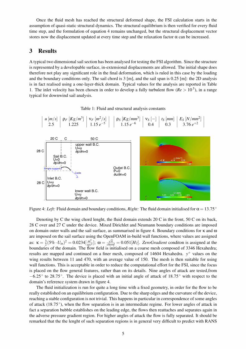
Once a pressure field reasonably close to the equilibrium has been calculated, this can be used forthe structural solver, which calculates the initial deflected position. This phase generally takes also along time: due to the very limited thickness of the fabric and the large displacement regime, the majorcontribution in the device’s stiffness derives from the non-linear membrane stiffness. This results in largeoscillations in the firsts time steps, which are then progressively damped as the analysis proceeds. Thegeneral behavior of the structure in this phase is exemplified in figure 3, where the displacement of asample node of the structure is reported versus the time-step.

Figure 3: nodal displacement versus time-step

When the stationary equilibrium for the first load vector is reached, the displacement is assigned tothe interface representing the sail in the fluid domain. This phase requires the use of under-relaxation,since large displacements can be imposed, which can introduce numerical instabilities in the calculation.The structural displacement is then linearly assigned as the fluid time proceeds. Being y0

s the structuraldisplacement vector, yn

F the displacement of the fluid interface at time-step n and α a scalar value, therelaxation is expressed as in equation 4. It was found that good values for α are of the same order ofmagnitude of the time-step value.

yn+1F = yn

F +α · (y0s − yn

F) (4)

4

Once the fluid mesh has reached the structural deformed shape, the FSI calculation starts in theassumption of quasi-static structural dynamics. The structural equilibrium is then verified for every fluidtime step, and the formulation of equation 4 remains unchanged, but the structural displacement vectorstores now the displacement updated at every time step and the relaxation factor α can be increased.

3 Results

A typical two dimensional sail section has been analysed for testing the FSI algorithm. Since the structureis represented by a developable surface, in-extensional displacements are allowed. The initial shape doestherefore not play any significant role in the final deformation, which is ruled in this case by the loadingand the boundary conditions only. The sail chord is 3 [m], and the sail span is 0.25 [m]: the 2D analysisis in fact realised using a one-layer-thick domain. Typical values for the analysis are reported in Table1. The inlet velocity has been chosen in order to develop a fully turbulent flow (Re > 10 5), in a rangetypical for downwind sail analysis.

Table 1: Fluid and structural analysis constants

u [m/s] ρF [Kg/m3] νF [m2/s] ρS [Kg/mm3] νS [−] tS [mm] ES [N/mm2]2.5 1.225 1.15 e−5 1.15 e−6 0.4 0.3 3.76 e+2

Figure 4: Left: Fluid domain and boundary conditions, Right: The fluid domain initialised for α= 13.75 ◦

Denoting by C the wing chord lenght, the fluid domain extends 20 C in the front, 50 C on its back,28 C over and 27 C under the device. Mixed Dirichlet and Neumann boundary conditions are imposedon domain outer walls and the sail surface, as summarised in figure 4. Boundary conditions for κ and ω

are imposed on the sail surface using the OpenFOAM in-build wall functions, where values are assignedas: κ = 3

2(5% ·Uin)2 = 0.0234[ m2

sec2 ]; ω =√

kchord

= 0.051[Hz]. ZeroGradient conditon is assigned at theboundaries of the domain. The flow field is initialised on a coarse mesh composed of 3346 Hexahedra;results are mapped and continued on a finer mesh, composed of 14604 Hexahedra. y+ values on thewing results between 11 and 470, with an average value of 150. The mesh is then suitable for usingwall functions. This is acceptable in order to reduce the computational effort for the FSI, since the focusis placed on the flow general features, rather than on its details. Nine angles of attack are tested,from−6.25 ◦ to 28.75 ◦. The device is placed with an initial angle of attack of 18.75 ◦ with respect to thedomain’s reference system drawn in figure 4.

The fluid initialization is run for quite a long time with a fixed geometry, in order for the flow to bereally established on an equilibrium configuration. Due to the sharp edges and the curvature of the device,reaching a stable configuration is not trivial. This happens in particular in correspondence of some anglesof attack (18.75 ◦), when the flow separation is in an intermediate regime. For lower angles of attack infact a separation bubble establishes on the leading edge, the flows then reattaches and separates again inthe adverse pressure gradient region. For higher angles of attack the flow is fully separated. It should beremarked that the the lenght of such separation regions is in general very difficult to predict with RANS

5

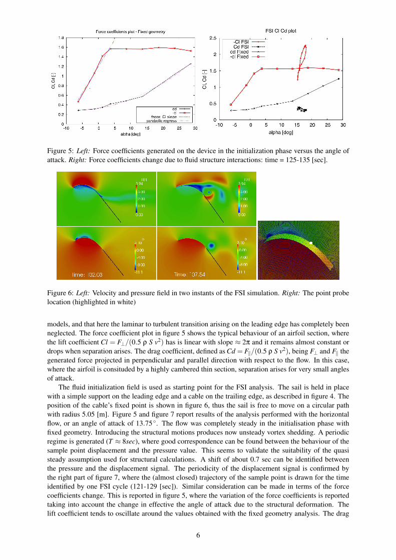
Figure 5: Left: Force coefficients generated on the device in the initialization phase versus the angle ofattack. Right: Force coefficients change due to fluid structure interactions: time = 125-135 [sec].

Figure 6: Left: Velocity and pressure field in two instants of the FSI simulation. Right: The point probelocation (highlighted in white)

models, and that here the laminar to turbulent transition arising on the leading edge has completely beenneglected. The force coefficient plot in figure 5 shows the typical behaviour of an airfoil section, wherethe lift coefficient Cl = F⊥/(0.5 ρ S v2) has is linear with slope ≈ 2π and it remains almost constant ordrops when separation arises. The drag coefficient, defined as Cd = F‖/(0.5 ρ S v2), being F⊥ and F‖ thegenerated force projected in perpendicular and parallel direction with respect to the flow. In this case,where the airfoil is consituded by a highly cambered thin section, separation arises for very small anglesof attack.

The fluid initialization field is used as starting point for the FSI analysis. The sail is held in placewith a simple support on the leading edge and a cable on the trailing edge, as described in figure 4. Theposition of the cable’s fixed point is shown in figure 6, thus the sail is free to move on a circular pathwith radius 5.05 [m]. Figure 5 and figure 7 report results of the analysis performed with the horizontalflow, or an angle of attack of 13.75 ◦. The flow was completely steady in the initialisation phase withfixed geometry. Introducing the structural motions produces now unsteady vortex shedding. A periodicregime is generated (T ≈ 8sec), where good correspondence can be found between the behaviour of thesample point displacement and the pressure value. This seems to validate the suitability of the quasisteady assumption used for structural calculations. A shift of about 0.7 sec can be identified betweenthe pressure and the displacement signal. The periodicity of the displacement signal is confirmed bythe right part of figure 7, where the (almost closed) trajectory of the sample point is drawn for the timeidentified by one FSI cycle (121-129 [sec]). Similar consideration can be made in terms of the forcecoefficients change. This is reported in figure 5, where the variation of the force coefficients is reportedtaking into account the change in effective the angle of attack due to the structural deformation. Thelift coefficient tends to oscillate around the values obtained with the fixed geometry analysis. The drag

6

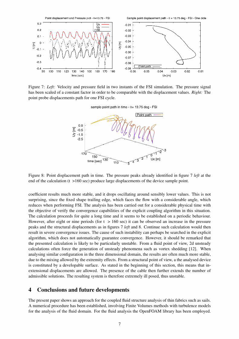
Figure 7: Left: Velocity and pressure field in two instants of the FSI simulation. The pressure signalhas been scaled of a constant factor in order to be comparable with the displacement values. Right: Thepoint probe displacements path for one FSI cycle.

Figure 8: Point displacement path in time. The pressure peaks already identified in figure 7 left at theend of the calculation (t >160 sec) produce large displacements of the device sample point.

coefficient results much more stable, and it drops oscillating around sensibly lower values. This is notsurprising, since the fixed shape trailing edge, which faces the flow with a considerable angle, whichreduces when performing FSI. The analysis has been carried out for a considerable physical time withthe objective of verify the convergence capabilities of the explicit coupling algorithm in this situation.The calculation proceeds for quite a long time and it seems to be established on a periodic behaviour.However, after eight or nine periods (for t > 160 sec) it can be observed an increase in the pressurepeaks and the structural displacements as in figures 7 left and 8. Continue such calculation would thenresult in severe convergence issues. The cause of such instability can perhaps be searched in the explicitalgorithm, which does not automatically guarantee convergence. However, it should be remarked thatthe presented calculation is likely to be particularly unstable. From a fluid point of view, 2d unsteadycalculations often force the generation of unsteady phenomena such as vortex shedding [12]. Whenanalysing similar configuration in the three dimensional domain, the results are often much more stable,due to the mixing allowed by the extremity effects. From a structural point of view, a the analysed deviceis constituted by a developable surface. As stated in the beginning of this section, this means that in-extensional displacements are allowed. The presence of the cable then further extends the number ofadmissible solutions. The resulting system is therefore extremely ill posed, thus unstable.

4 Conclusions and future developments

The present paper shows an approach for the coupled fluid structure analysis of thin fabrics such as sails.A numerical procedure has been established, involving Finite Volumes methods with turbulence modelsfor the analysis of the fluid domain. For the fluid analysis the OpenFOAM library has been employed.

7

The structural domain is analysed with shells finite elements, using the Shelddon package. The couplingis performed in an ALE framework, where the structural displacement is diffused in the fluid domainusing a Laplacian operator. The structural deformation is modeled with a ’quasi static’ assumption,which seems to produce acceptable results even when the flow becomes unsteady. Results have beenreported and discussed for a two-dimensional sail section held in place by a simple support and a cable.The flow field has been initialised with the fixed sail section, and typical force coefficient plot have beenobtained. The FSI coupled analysis has then been performed; results have been compared and discussed.In particular, the presented approach uses an explicit coupling algorithm, where the structure is analysedin the quasi-static assumption. The presented test case was representative of a critical situation, whereboth the fluid and the structural calculations are likely to be unstable. Despite of this, the analysis wascarried out for a reasonable time with no remarkable convergence issues. It can then be concluded thatthe presented approach results suitable for the dynamic analysis of three dimensional sails. In the nearfuture fully three dimensional calculations will be carried out and possibly validated with experimentaldata. Performing three dimensional calculation would eventually confirm the evaluation of the impact ofwrinkling on the flow, which was started in [12]. From a computing perspective, several improvementscan be made. In the present stage the FSI communication allows only single process calculations, thusthe parallel computing capabilities of OpenFOAM are not exploited. Only conforming meshes are used,whereas different mesh distributions may be suitable for the fluid and the structural analysis.

References

[1] K.J. Bathe. Finite Element Procedures in Engineering Analysis, Prentice-Hall, 1996.

[2] D. Chapelle, K.J. Bathe. The Finite Element Analysis of Shells: Fundamentals, Springer, 2003.

[3] S. Collie, M. Gerritsen, P. Jackson. A review of turbulence modelling for use in sail flow analysis , School ofEngineering report 603, the University of Auckland, 53 pages, 2001

[4] M. Durand, Y. Roux, A. Leroyer, M. Visonneau. Unsteady numerical simulations of downwind sails, In-nov’Sail conference, The Royal institution of Naval Architects, 10 pages, 2010.

[5] C. Kassiotis. Which strategy to move the mesh in the Computational Fluid Dy-

namic code OpenFOAM, Report École Normale Supérieure de Cachan. Available online:http://perso.crans.org/kassiotis/openfoam/movingmesh.pdf, 2008

[6] Menter, F. R., Two-Equation Eddy-Viscosity Turbulence Models for Engineering Applications, AIAA Journal,Vol. 32, No. 8, pp. 1598-1605, August 1994

[7] www.openfoam.com.

[8] N. Parolini, A. Quarteroni. Mathematical models and numerical simulations for the America’s cup, MOXreport, Politecnico di Milano 36 pages, 2004.

[9] H. Renschz, O. Muller, K. Graf. FlexSail - A fluid structure interaction program for the investigation of Spin-

nakers Innov’Sail conference, The Royal institution of Naval Architects, 14 pages, 2008.

[10] H. Renschz, K. Graf. Fluid Structure Interaction Simulation of Spinnakers - Getting closer to reality, In-nov’Sail conference, The Royal institution of Naval Architects, 9 pages, 2010.

[11] Shelddon is a finite element library developped at INRIA and registered at the Agence pour la Protection

des Programmes under ref: IDDN.FR.001.030018.000.S.P.2010.000.20600. The base of the program is open-Source and available online: http://www- rocq.inria.fr/modulef/.

[12] D. Trimarchi, S.R. Turnock, D. Chapelle, D. Taunton. The use of shell elements to capture sail wrinkles,

and their influence on aerodynamic load, Innov’Sail conference, The Royal institution of Naval Architects, 12pages, 2010.

[13] C.G. Wang, H.F. Tan, X.W. Du, Z.M. Wan. Wrinkling prediction of rectangular shell-membrane under trans-

verse in-plane displacement,International journal of Solid and Structures, Vol.44, pages 6507-6516, 2007.

[14] Y.W. Wong, S. Pellegrino. Wrinkled membranes: Experiments; Analytical model; Numerical simulations,Journal of Mechanics of Materials and Structures, Vol.1, 24, 36, 34 pages, 2006.

8