Intellectual Property Rights Policy, Competition and Innovation

The MIT Faculty has made this article openly available. Please share how this access benefits you. Your story matters.

Citation Acemoglu, Daron, and Ufuk Akcigit. “INTELLECTUAL PROPERTYRIGHTS POLICY, COMPETITION AND INNOVATION.” Journal of theEuropean Economic Association 10.1 (2012): 1-42.

As Published http://dx.doi.org/10.1111/j.1542-4774.2011.01053.x

Publisher Wiley Blackwell

Version Author's final manuscript

Citable link http://hdl.handle.net/1721.1/72048

Terms of Use Creative Commons Attribution-Noncommercial-Share Alike 3.0

Detailed Terms http://creativecommons.org/licenses/by-nc-sa/3.0/

Intellectual Property Rights Policy,Competition and Innovation∗

Daron AcemogluMassachusetts Institute of Technology

Ufuk AkcigitUniversity of Pennsylvania

May 8, 2011

Abstract

To what extent and in what form should the intellectual property rights (IPR) of innovatorsbe protected? Should a company with a large technology lead over its rivals receive thesame IPR protection as a company with a more limited advantage? The analysis of thesequestions necessitates a dynamic framework for the study of the interactions between IPRand competition, in particular to understand the impact of such policies on future incentives.In this paper, we develop such a framework. The economy consists of many industries andfirms engaged in cumulative (step-by-step) innovation. IPR policy regulates whether followersin an industry can copy (or license or build upon) the technology of the leader. With fullpatent protection, followers can catch up to the leader in their industry only by making thesame innovation(s) themselves (or by full licensing). We prove the existence of a steady-state equilibrium in a baseline environment and characterize some of its properties. We thenquantitatively investigate the implications of different types of IPR policy on the equilibriumgrowth rate and welfare. The most important result from this exercise is that full patentprotection is not optimal (welfare maximizing); instead, optimal policy involves state-dependentIPR protection, providing greater protection to technology leaders that are further ahead thanthose that are close to their followers. This form of the optimal policy results from the impactof policy on dynamic incentives, in particular from a form of “trickle-down”effect: providinggreater protection to firms that are further ahead of their followers than a certain thresholdincreases the R&D incentives also for all technology leaders that are less advanced than thisthreshold.

Keywords: competition, economic growth, endogenous growth, industry structure, inno-vation, intellectual property rights, licensing, patents, research and development, trickle-down.

JEL classification: O31, O34, O41, L16.

∗We thank conference and seminar participants at the FBBVA Lecture at 2011 ASSA conference in Denver,the Canadian Institute of Advanced Research, EPFL Technology Policy Conference, European Science Days,MIT, National Bureau of Economic Research Economic Growth and Productivity Groups, Toulouse InformationTechnology Network, University of Pennsylvania, University of Toronto and Philippe Aghion, Gino Gancia,Bronwyn Hall, Sam Kortum and Suzanne Scotchmer for useful comments. Financial support from the ToulouseInformation Technology Network is gratefully acknowledged.

1 Introduction

What is the optimal extent and form of intellectual property rights (IPR) protection? Should

a firm with a large technology lead receive the same IPR protection as a company with a

more limited technological lead, or should IPR policy be coupled with antitrust and used to

limit the monopoly power of technology leaders? Despite broad consensus that innovation is

central to the long-run performance of an economy, there is no consensus on the answers to

such questions. A large literature on IPR (discussed below) focuses on the static trade-offs

between the positive incentive benefits of IPR protection and its costs in terms of reducing

competition and increasing markups. In this paper, we argue that dynamic trade-offs between

IPR protection and competition, which have so far been overlooked, may be equally or more

important for developing answers to these questions.

These issues and the importance of these questions are highlighted by several recent high-

profile cases.1 For example, motivated by antitrust concerns, a recent ruling of the European

Commission ordered Microsoft to share secret information about its operating system and

products with other software companies (New York Times, December 22, 2004). Similar issues

were also central to the US Department of Justice (DOJ) case against Microsoft, which started

on May 18th, 1998 and ultimately resulted in a ruling against Microsoft. Figures 1 and 2 show

the evolution of R&D by Microsoft and by other top 10 publicly traded R&D investors in the

IT sector relative to the sector average before and after the start of the DOJ case.2

[Figure 1 & 2 here]

The relative R&D spending by Microsoft and other industry leaders, which had been

steadily– perhaps even exponentially– increasing since the mid-80s, appear to decline after

the DOJ action. While one might expect R&D by Microsoft to slow down for a variety of

reasons, it is not obvious why there should be a relative decline in the R&D of other top

companies, since they partly benefited from the weakening of, and the restrictions imposed on,

Microsoft. This relative decline may have been caused by a slowdown in the R&D activities

of these other companies or an increase in the R&D investments of smaller IT firms (or by

1 In addition to the Microsoft case, the issue of technological lead has been central in the Department ofJustice investigations of Intel (New York Times, May 11, 2009) and the debates about Google’s market share(New York Times, February 21, 2009).

2All data are from COMPUSTAT. Top 10 firms is determined by the highest 10 R&D investors (exceptMicrosoft) in 1995. The patterns shown in Figures 1 and 2 are very similar if we use in that top 10 investors in2000 or 1990, or if we benchmark it to the median of the industry rather than the mean. Top 10 investors inFigure 2 are: CA Inc, Continuum Inc, Intergraph Corp, Sterling Software Inc, Oracle Inc, Adobe Inc, SymantecCorp, Electronic Arts Inc, Sybase Inc, Intuit Inc.

1

entirely different and unrelated factors). To investigate these issues more systematically, we

need a dynamic equilibrium framework where R&D activities of different types of firms might

be affected by a change in IPR and competition policy.

Our framework builds on and extends the step-by-step innovation models of Aghion, Harris

and Vickers (1997) and Aghion, Harris, Howitt and Vickers (2001), where a number of (typi-

cally two) firms engage in price competition within an industry and undertake R&D in order

to improve their production technology. The technology gap between the firms determines

the extent of the monopoly power of the leader, and hence the price markups and profits.

The purpose of R&D by the follower is to catch up and surpass the leader (as in standard

Schumpeterian models of innovation, e.g., Reinganum, 1981, 1985, Aghion and Howitt, 1992,

Grossman and Helpman, 1991), while the purpose of R&D by the leader is to escape the

competition of the follower and increase its markup and profits. Despite the dynamic nature

of these models, their policy implications are still mostly based on the same static trade-off

mentioned above. For this reason, for example, Aghion, Harris, Howitt and Vickers (2001,

p. 481) conjecture that IPR protection should be limited and particularly so for firms with

larger technological leads over their rivals (which face less competition and thus have greater

monopoly power).

We extend these existing models in several directions. Most importantly, we explicitly

introduce state-dependent patent/IPR protection policy, meaning a policy that makes the

extent of patent or intellectual property rights protection conditional on the technology gap

between different firms in the industry. As in racing-type models in general (e.g., Harris and

Vickers, 1985, 1987, Budd, Harris and Vickers, 1993), a large gap between the leader and

the follower discourages R&D by both. Consequently, overall R&D and technological progress

are greater when the technology gap between the leader and the follower is relatively small.3

One may then expect that full patent protection may be suboptimal in a world of step-by-

step competition and permitting followers to copy or use the leaders’technologies would be

particularly beneficial in industries where there is a large technology gap between leaders and

followers.4 However, crucially, this reasoning ignores the dynamic incentive effects, which are

our main focus in this paper and emerge more clearly when IPR policy is explicitly state-

dependent.

Our analysis establishes that the opposite of the above conjecture is always true in such

3Aghion, Bloom, Blundell, Griffi th and Howitt (2005) provide empirical evidence from British industriesconsistent with the view R&D increases when there is a smaller technological gap between firms. See alsoAghion and Griffi th (2007).

4This is indeed the basis of Aghion, Harris, Howitt and Vickers’s conjecture.

2

a dynamic equilibrium framework: optimal IPR policy should provide greater protection to

technologically more advanced leaders. Underlying this result is what we refer to as the trickle-

down of incentives: providing relatively low protection to firms with limited leads and greater

protection to those that have greater leads not only improves the incentives of firms that are

technologically advanced, but also encourages R&D by those that have limited leads because

of the prospect of reaching levels of technology gaps associated with greater protection. A

corollary of this result is that full IPR protection is not optimal, and there should be limited

(but state-dependent) IPR protection for firms with only limited technology leads over their

rivals.

More specifically, we show that in contrast to the standard disincentive effects of uniform

relaxation of IPR policy, state-dependent relaxation that provides greater protection to tech-

nologically more advanced firms creates a positive incentive effect. This is because when a

particular state for the technology leader (say being n∗ steps ahead of the follower) becomes

more profitable, this increases the incentives to perform R&D not only for leaders that are

n∗ − 1 steps ahead, but for all leaders with a lead of size n ≤ n∗ − 1. It is this trickle-down

effect that generates the positive incentive effect and makes state-dependent IPR, with greater

protection for firms that are technologically more advanced than their rivals, preferable to

uniform IPR.

We start with a partial equilibrium model, which under some simplifying assumptions al-

lows an explicit characterization of the trickle-down effect. We then provide a richer dynamic

general equilibrium framework which allows a variety of different assumptions on how inno-

vation depends on R&D by technology leaders and followers. Our baseline model focuses on

quick catch-up, meaning that a follower can catch up with the technology leader with a single

innovation regardless of the size of the gap between them. For this environment, we establish

the existence of a stationary equilibrium and characterize some of its properties. We then

study the form of optimal (welfare maximizing) IPR and competition policy quantitatively.

The same effects as in the partial equilibrium analysis make state-dependent relaxation of IPR

optimal. Quantitatively, we find that optimal state-dependent IPR policy can increase the

growth rate of the economy from 1.86% to 2.04%, and does so with fewer workers employed

in the R&D sector (because R&D workers are reallocated towards firms where their efforts

directly lead to productivity growth). In contrast, uniform relaxation of IPR policy reduces

both welfare and growth. These patterns are quite robust to different parameter values.

We next show how the framework can be extended to study these issues under alternative

assumptions, in particular, assuming slow catch-up so that followers close the gap between

3

themselves and technology leaders only gradually. The presence of slow catch-up also enables

us to introduce different types of R&D efforts and different dimensions of IPR policy, in

particular, licensing and patent infringement fees.5 We show that the trickle-down effect and

the result that optimal IPR policy should be state-dependent and provide greater protection

to technologically more advanced firms are robust in these alternative environments. In most

cases, optimal IPR policy also increases growth by a similar magnitude to our baseline model

(though in some cases, it increases welfare but not necessarily growth).6

Our paper is a contribution both to the IPR protection and the endogenous growth lit-

eratures. Previous work has focused on the static trade-off between ex-post monopoly rents

and ex-ante R&D incentives (e.g., Arrow, 1962, Reinganum, 1981, Tirole, 1988, Romer, 1990,

Grossman and Helpman, 1991, Aghion and Howitt, 1992, Green and Scotchmer, 1995, Scotch-

mer, 1999, Gallini and Scotchmer, 2002, O’Donoghue and Zweimuller, 2004).7 Much of the

literature discusses the trade-off between these two forces to determine the optimal length and

breadth of patents. For example, Klemperer (1990) and Gilbert and Shapiro (1990) show that

optimal patents should have a long duration in order to provide inducement to R&D, but a

narrow breadth so as to limit monopoly distortions. A number of other papers, for example,

Gallini (1992) and Gallini and Scotchmer (2002), reach opposite conclusions.

Another branch of the literature, including the seminal paper by Scotchmer (1999) and

the recent interesting papers by Llobet, Hopenhayn and Mitchell (2006) and Hopenhayn and

Mitchell (2001, 2011), adopts a mechanism design approach to the determination of the optimal

patent and intellectual property rights protection system. For example, Scotchmer (1999)

derives the patent renewal system as an optimal mechanism in an environment where the cost

and value of different projects are unobserved and the main problem is to decide which projects

should go ahead. Llobet, Hopenhayn and Mitchell (2006) consider optimal patent policy in the

context of a model of sequential innovation with heterogeneous quality and private information.

They show that allowing for a choice from a menu of patents will be optimal in this context.

5 In particular, in this regime, we allow firms to undertake frontier as well as catch-up R&D. With frontierR&D, they can build on the technology leader’s knowledge base and, if successful, they immediately surpass theleader, but might be liable for a patent infringement fee.We also allow followers to license the innovation of the technology leader by paying a prespecified license

fee– i.e., a “compulsory licensing” where the license fee is determined by IPR policy. We also show thatvoluntary licensing agreements would not achieve the same results, so our analysis establishes a potential needfor compulsory licensing policy. Previous work emphasizing importance of compulsory licensing includes Tandon(1982), Gilbert and Shapiro (1990), and Kremer (2002). See Moser and Voena (2011) for a recent empiricalinvestigation.

6We also show that both licensing and the possibility of frontier R&D (subject to infringement fees) con-tributes to growth and welfare.

7Boldrin and Levine (2004, 2008) or Quah (2003) argue that patent systems are not necessary for innovation.

4

Hopenhayn and Mitchell (2011) build on an earlier version of our paper, Acemoglu and Akcigit

(2006), and derive a form of trickle-down effect using a mechanism design approach in a model

with recurring innovations.

Our paper also extends Aghion, Harris and Vickers (1997) and Aghion, Harris, Howitt

and Vickers (2001).8 Although our model builds on these papers, it also differs from them

in a number of significant ways. First and most importantly, we introduce state-dependent

IPR policy. Second, we also introduce and analyze the slow catch-up regime, and in this

context, we allow for compulsory licensing and for leapfrogging, which makes the followers

directly contribute to the economic growth. We provide a full quantitative analysis of state-

dependent IPR policy under these different scenarios. Third, our economy is a full general

equilibrium model with competition between production and R&D for scarce labor.9 Finally,

we provide a general existence result and a number of analytical results for the general model

(with or without IPR policy), while previous literature has focused on the special cases where

innovations are either “drastic”(so that the leader never undertakes R&D) or very small, and

has not provided existence or general characterization results for steady-state equilibria.

Lastly, our results are also related to the literature on tournaments and races, for example,

Fudenberg, Gilbert, Stiglitz and Tirole (1983), Harris and Vickers (1985, 1987), Choi (1991),

Budd, Harris and Vickers (1993), Taylor (1995), Fullerton and McAfee (1999), Baye and Hoppe

(2003), and Moscarini and Squintani (2004). This literature considers the impact of endogenous

or exogenous prizes on effort in tournaments, races or R&D contests. In terms of this literature,

state-dependent IPR policy can be thought of as “state-dependent handicapping”of different

players (where the state variable is the gap between the two players in a dynamic tournament).

To the best of our knowledge, these types of schemes have not been considered in this literature.

The rest of the paper is organized as follows. Section 2 introduces the partial equilibrium

model and analytically demonstrates the trickle-down effect. Section 3 presents our baseline

environment (where a successful innovation by followers closes the entire gap with technol-

ogy leaders in one step, i.e., there is quick catch-up). Section 4 proves the existence of a

steady-state equilibrium and characterizes some of its key properties under both uniform and

state-dependent IPR policy. Section 5 defines the social welfare objective and outlines our

8Segal and Whinston (2007) analyze the impact of anti-trust policy on economic growth in a related modelof step-by-step innovation.

9This general equilibrium aspect is introduced to be able to close the model economy without unrealisticassumptions and makes our economy more comparable to other growth models (Aghion, Harris, Howit andVickers, 2001, assume a perfectly elastic supply of labor). We show that the presence of general equilibriuminteractions does not significantly complicate the analysis and it is still possible to characterize the steady-stateequilibrium.

5

quantitative methods. Section 6 characterizes the structure of optimal IPR policy quantita-

tively. Section 7 extends the model to allow for slow catch-up, compulsory license fees and

leapfrogging, and quantitatively characterizes the structure of optimal IPR policy under dif-

ferent combinations of these policies. Section 8 concludes, while the Appendix contains the

proofs of all the results stated in the text.

2 A Partial Equilibrium Illustration

We first illustrate the main economic force in this paper, the trickle-down effect, using a partial

equilibrium model. Consider the following infinite horizon, step-by-step R&D race between two

competing firms in continuous time. Each firm maximizes the expected net present discounted

value of “net profits,”defined as operating profit minus R&D cost,

Et∫ ∞t

exp (−r (s− t)) [πi (s)− Φi (s)] ds,

where Et denotes expectation at time t, r > 0 is the interest rate, πi (t) is the instantaneous

operating profit flow and Φi (t) represents the R&D cost of firm i at time t. In this game, firm

i ∈ {1, 2} invests in R&D to advance its position relative to its rival i′ 6= i. Suppose that the

positions of both firms in this race can be characterized by integer values on the real line, and

denote the distance of firm i from its rival at time t by ni (t). In the partial equilibrium model,

we simplify the analysis by following Aghion, Harris, Howitt and Vickers (2001) and Aghion,

Bloom, Blundell, Griffi th and Howitt (2005) in assuming that the maximum technology gap

between a leader and a follower is 2; this assumption is relaxed in the full general equilibrium

model analyzed in the rest of the paper. For now it simplifies the analysis by ensuring that

the relative position of firm i can take five possible values, ni (t) ∈ NI ≡ {−2,−1, 0, 1, 2}. Letus denote the absolute gap between the firms by n (t) ≡ max {ni (t) , n−i (t)}, and suppress thetime subscripts to simplify notation.

The payoffs in this game are assumed to be stationary and only a function of the relative

distance between the firms, thus represented by π : NI → R+ (see equation (20) in Section 3).

Here πni ≥ 0 is simply the instantaneous payoff that firm i obtains when its distance from its

competitor is ni at time t and assumed to be a strictly increasing function of ni. To advance

its relative position, firm i invests in R&D, which determines the Poisson rate of arrival of

innovation, xi ∈ R+. Let us also assume that the cost of R&D is linear in the arrival rate

of innovation, i.e., Φ (xi) = φxi, with φ > 0 (again see below for more general formulations).

Each successful innovation is patented and advances firm i’s state (relative position) by one

6

step, so that following a successful innovation by firm i at time t we have: ni (t+) = ni (t) + 1

(where ni (t+) stands for ni immediately following time t).

IPR policy governs the expected length of a patent. For simplicity, we model patent length

by assuming that it terminates at a Poisson rate. Crucially for our focus, IPR policy is state

dependent, and we represent it by the function: η : NI→ R+. Here η (n) ≡ ηn <∞ is the flow

rate at which the patent terminates (patent protection is removed) for a technology leader that

is n steps ahead. When ηn = 0, this implies that there is full protection at technology gap n,

in the sense that patent protection will never be removed. In contrast, ηn → ∞ implies that

patent protection is removed immediately once technology gap n is reached. When the patent

protection is removed, the firm that is behind copies the technology of its competitor and both

firms end up neck-and-neck, i.e., n = 0.

Finally, we take the interest rate r as exogenous and assume that it satisfies r <

(πn − πn−1) /4φ for each n ∈ NI. This assumption ensures positive R&D by each firm when

ηn = 0. Throughout we will focus on (stationary) Markov Perfect Equilibria (MPE), where

strategies (R&D decisions) are only functions of the payoff-relevant state, which is n ∈ NI. A

more formal definition of the MPE in the general equilibrium environment is given below.

The MPE can be characterized by writing the value functions of each firm as a function of

the state n ∈ NI. These value functions are given by the following recursions:

rv2 = π2 + x−2 [v1 − v2] + η2 [v0 − v2] , (1)

rv1 = maxx1≥0

{π1 − φx1 + x1 [v2 − v1] + x−1 [v0 − v1] + η1 [v0 − v1]} , (2)

rv0 = maxx0≥0

{π0 − φx0 + x0 [v1 − v0] + x0 [v−1 − v0]} , (3)

rv−1 = maxx−1≥0

{π−1 − φx−1 + x−1 [v0 − v−1] + x1 [v−2 − v−1] + η1 [v0 − v−1]} , (4)

rv−2 = maxx−2≥0

{π−2 − φx−2 + x−2 [v−1 − v−2] + η2 [v0 − v−2]} . (5)

In all equations, the first term represents current profits. In equations (2)-(5), the second term

substracts R&D costs from current profits, the third term represents the fact that the firm will

successfully innovate at the flow rate xn and increase its position by one step. The fourth term

incorporates the change in value due to an innovation by the rival firm. In equations (1) and (2)

the last term is the change in value for the leader due to patent expiration, which takes place

at the rate ηn, while in (4) and (5) is the change in value for the follower. Finally, equation (3)

has the same interpretation except that now n = 0 and the two firms are neck-and-neck and

thus there is no IPR policy (and the flow rate of innovation of the other firm is denoted by x0,

and naturally, in a symmetric equilibrium, we will have x0 = x0). Note also that in equations

7

(1) and (5), we used the fact that a two-step ahead firm does not undertake any R&D since it

has already achieved the maximum feasible lead.

We will now characterize the MPE under two different policy environments: uniform and

state-dependent IPR policy.

Uniform IPR Policy. Uniform IPR policy corresponds to the case where ηn = η <

∞. Consequently, optimal R&D decisions in equations (2)-(5) can be solved out as (see the

Appendix):

x∗−2 = max

{−4η +

π2 − π−2

φ− 4r, 0

}, x∗−1 = max

{−3η +

π1 − π−2

φ− 3r, 0

},

x∗0 = max

{−2η +

π0 − π−2

φ− 2r, 0

}, and x∗1 = max

{−η +

π−1 − π−2

φ− r, 0

}.

Inspection of these expressions immediately establishes the following result:

Proposition 1 Under uniform IPR policy regime, any relaxation of IPR policy (away from

η = 0) creates a “disincentive effect”and reduces all R&D levels.

State-dependent IPR Policy. We next consider state-dependent policy where the patent

protection of a technology leader depends on the technology gap, n. Optimal R&D decisions

can now be written out as (see the Appendix):

x∗−2 = max

{−4η2 +

π2 − π−2

φ− 4r, 0

}, x∗−1 = max

{−η1 − 2η2 +

π1 − π−2

φ− 3r, 0

},

x∗0 = max

{−2η2 +

π0 − π−2

φ− 2r, 0

}, and x∗1 = max

{η1 − 2η2 +

π−1 − π−2

φ− r, 0

}.

Inspection of these expressions shows that, in contrast to the uniform IPR case, relaxing

patent protection can increase the R&D effort of the one-step leader, x∗1. In particular, this

can be accomplished by providing a lower protection in the current state (higher η1) and/or a

higher protection upon a successful innovation (lower η2).

Proposition 2 Under state-dependent IPR policy regime, relaxing IPR policy (away from

ηn = 0) by weakening current protection (i.e., increasing η1) creates a “positive incentive

effect”and increases x∗1.

Whether optimal IPR policy will involve η1 > 0 and/or η2 > 0 now depends on the social

returns from xn’s. For example, if x1 is socially more beneficial than x−1, η1 > 0 will always

be preferred. In the context of our general equilibrium model, this will always be the case.

Proposition 2 provides a preview of these results.

8

3 General Equilibrium Framework

We now describe our baseline dynamic general equilibrium model. To maximize continuity

with the previous literature and to provide the sharpest theoretical characterization results,

our baseline model assumes quick catch-up, meaning that one innovation by a follower is suf-

ficient to close the gap with the technology leader in the industry. The characterization of

the equilibrium in this environment under the different policy regimes is presented in the next

section. Alternative assumptions on the form of catch-up are investigated in Section 7.

3.1 Preferences and Technology

Consider the following continuous time economy with a unique final good. The economy is

populated by a continuum of 1 individuals, each with 1 unit of labor endowment, which they

supply inelastically. Preferences at time t are given by

Et∫ ∞t

exp (−ρ (s− t)) logC (s) ds, (6)

where Et denotes expectations at time t, ρ > 0 is the discount rate and C (t) is consumption

at date t. The logarithmic preferences in (6) facilitate the analysis, since they imply a simple

relationship between the interest rate, growth rate and the discount rate (see (7) below).

Let Y (t) be the total production of the final good at time t. We assume that the economy

is closed and the final good is used only for consumption (i.e., there is no investment), so that

C (t) = Y (t). The standard Euler equation from (6) then implies that

g (t) ≡ C (t)

C (t)=Y (t)

Y (t)= r (t)− ρ, (7)

where this equation defines g (t) as the growth rate of consumption and thus output, and r (t)

is the interest rate at date t.

The final good Y is produced using a continuum 1 of intermediate goods according to the

Cobb-Douglas production function

lnY (t) =

∫ 1

0ln y (j, t) dj, (8)

where y (j, t) is the output of jth intermediate at time t. Throughout, we take the price of the

final good as the numeraire and denote the price of intermediate j at time t by p (j, t). We

also assume that there is free entry into the final good production sector. These assumptions,

together with the Cobb-Douglas production function (8), imply that the final good sector has

9

the following demand for intermediates

y (j, t) =Y (t)

p (j, t), ∀j ∈ [0, 1] . (9)

Intermediate j ∈ [0, 1] comes in two different varieties, each produced by one of two

infinitely-lived firms. We assume that these two varieties are perfect substitutes and these

firms compete a la Bertrand.10 Firm i = 1 or 2 in industry j has the following technology

y (j, t) = qi (j, t) li (j, t) (10)

where li (j, t) is the employment level of the firm and qi (j, t) is its level of technology at

time t. Each consumer in the economy holds a balanced portfolio of the shares of all firms.

Consequently, the objective function of each firm is to maximize expected profits.

The production function for intermediate goods, (10), implies that the marginal cost of

producing intermediate j for firm i at time t is

MCi (j, t) =w (t)

qi (j, t)(11)

where w (t) is the wage rate in the economy at time t.

When this causes no confusion, we denote the technology leader in each industry by i and

the follower by −i, so that we have:

qi (j, t) ≥ q−i (j, t) .

Bertrand competition between the two firms implies that all intermediates will be supplied by

the leader at the “limit”price:11

pi (j, t) =w (t)

q−i (j, t). (12)

Equation (9) then implies the following demand for intermediates:

y (j, t) =q−i (j, t)

w (t)Y (t) . (13)

10A more general case would involve these two varieties being imperfect substitutes, for example, with theoutput of intermediate j produced as

y (j, t) =[ϕy1 (j, t)

σ−1σ + (1− ϕ) y2 (j, t)

σ−1σ

] σσ−1

,

with σ > 1. The model analyzed in the text corresponds to the limiting case where σ →∞. Our results can beeasily extended to this more general case with any σ > 1, but at the cost of additional notation. We thereforeprefer to focus on the case where the two varieties are perfect substitutes. It is nonetheless useful to bear thisformulation with imperfect substitutes in mind, since it facilitates the interpretation of “distinct” innovationsby the two firms (when the follower engages in “catch-up”R&D).11 If the leader were to charge a higher price, then the market would be captured by the follower earning

positive profits. A lower price can always be increased while making sure that all final good producers stillprefer the intermediate supplied by the leader i rather than that by the follower −i, even if the latter weresupplied at marginal cost. Since the monopoly price with the unit elastic demand curve is infinite, the leaderalways gains by increasing its price, making the price given in (12) the unique equilibrium price.

10

3.2 Technology, R&D and IPR Policy under Quick Catch-up

R&D by the leader or the follower stochastically leads to innovation. We assume that when

the leader innovates, its technology improves by a factor λ > 1.

The follower, on the other hand, can undertake R&D to catch up with the frontier tech-

nology. We will call this type of R&D as catch-up R&D.12 Catch-up R&D can be thought of

R&D to discover an alternative way of performing the same task as the current leading-edge

technology. Because this innovation applies to the follower’s variant of the product (recall

footnote 10) and results from its own R&D efforts, we assume in our baseline framework that

it does not constitute infringement on the patent of the leader.13

R&D by the leader and follower may have different costs and success probabilities. We

simplify the analysis by assuming that both types of R&D have the same costs and the same

probability of success. In particular, in all cases, we assume that innovations follow a controlled

Poisson process, with the arrival rate determined by R&D investments. Each firm (in every

industry) has access to the following R&D technology:

xi (j, t) = F (hi (j, t)) , (14)

where xi (j, t) is the flow rate of innovation at time t and hi (j, t) is the number of workers

hired by firm i in industry j to work in the R&D process at t. This specification implies that

within a time interval of ∆t, the probability of innovation for this firm is xi (j, t) ∆t+ o (∆t).

We assume that F is twice continuously differentiable and satisfies F ′ (·) > 0, F ′′ (·) < 0,

F ′ (0) < ∞ and that there exists h ∈ (0,∞) such that F ′ (h) = 0 for all h ≥ h. The

assumption that F ′ (0) < ∞ implies that there is no Inada condition when hi (j, t) = 0. The

last assumption, on the other hand, ensures that there is an upper bound on the flow rate of

innovation (which is not essential but simplifies the proofs). Recalling that the wage rate for

labor is w (t), the cost for R&D is therefore w (t)G (xi (j, t)) where

G (xi (j, t)) ≡ F−1 (xi (j, t)) , (15)

and the assumptions on F immediately imply that G is twice continuously differentiable and

satisfies G′ (·) > 0, G′′ (·) > 0, G′ (0) > 0 and limx→xG′ (x) =∞, where

x ≡ F(h)

(16)

12This contrasts with frontier R&D introduced in Section 7, which will allow the follower to leapfrog theleader.13We allow for infringement in Section 7.

11

is the maximal flow rate of innovation (with h defined above).

We next describe the evolution of technologies within each industry. Suppose that leader i

in industry j at time t has a technology level of

qi (j, t) = λnij(t), (17)

and that the follower −i’s technology at time t is

q−i (j, t) = λn−ij(t), (18)

where nij (t) ≥ n−ij (t) and nij (t), n−ij (t) ∈ Z+ denote the technology rungs of the leader and

the follower in industry j. We refer to nj (t) ≡ nij (t)−n−ij (t) as the technology gap in industry

j. If the leader undertakes an innovation within a time interval of ∆t, then its technology

increases to qi (j, t+ ∆t) = λnijt+1 and the technology gap rises to nj (t+ ∆t) = nj (t) + 1

(the probability of two or more innovations within the interval ∆t will be o (∆t), where o (∆t)

represents terms that satisfy lim∆t→0 o (∆t) /∆t).

In our baseline model, we assume that there is quick catch-up between followers and leaders.

Namely, when the follower is successful in catch-up R&D within the interval ∆t, then its

technology improves to

q−i (j, t+ ∆t) = λnijt ,

and thus it catches up with the leader immediately (regardless of how large the technology

gap was). In this case, the technology gap variable becomes njt+∆t = 0 upon a successful

innovation by the follower.14

In addition to catching up with the technology frontier with their own R&D, followers can

also copy the technology frontier because IPR policy is such that some patents expire. In

particular, we assume that patents expire at some policy-determined Poisson rate η, and after

expiration, followers can costlessly copy the frontier technology, jumping to q−i (j, t+ ∆t) =

λnijt .15 As in the partial equilibrium model in Section 2, IPR policy governs the length of the

patent and we allow it to be state dependent, so it is represented by the following function:

η : N→ R+

Here η (n) ≡ ηn < ∞ is the flow rate at which the patent protection is removed from a

technology leader that is n steps ahead of the follower. When ηn = 0, this implies that there is14 In Section 7, we will replace this assumption with slow catch-up where one innovation enables the follower

to proceed by one step.15Alternative modeling assumptions on IPR policy, such as a fixed patent length of T > 0 from the time

of innovation, are not tractable, since they lead to value functions that take the form of delayed differentialequations.

12

full protection at technology gap n, in the sense that patent protection will never be removed.

In contrast, ηn → ∞ implies that patent protection is removed immediately once technology

gap n is reached. Our formulation imposes that η ≡{η1, η2, ...} is time-invariant. Given thisspecification, we can now write the law of motion of the technology gap in industry j as follows:

nj (t+ ∆t) =

nj (t) + 1

0

nj (t)

with probability

with probability

with probability

xi (j, t) ∆t+ o (∆t)(x−i (j, t) + ηnj(t)

)∆t+ o (∆t)

1−(xi (j, t) + x−i (j, t) + ηnj(t)

)∆t− o (∆t))

.

(19)

Here o (∆t) again represents second-order terms, in particular, the probabilities of more than

one innovations within an interval of length ∆t. The terms xi (j, t) and x−i (j, t) are the flow

rates of innovation by the leader and the follower; and ηnj(t) is the flow rate at which the

follower is allowed to copy the technology of a leader that is nj (t) steps ahead. Intuitively, the

technology gap in industry j increases from nj (t) to nj (t) + 1 if the leader is successful. The

firms become “neck-and-neck”when the follower comes up with an alternative technology to

that of the leader (flow rate x−i (j, t)) or the patent expires at the flow rate ηnj .

3.3 Profits

We next write the instantaneous “operating”profits for the leader (i.e., the profits exclusive

of R&D expenditures). Profits of leader i in industry j at time t are

Πi (j, t) = [pi (j, t)−MCi (j, t)] yi (j, t)

=

(w (t)

q−i (j, t)− w (t)

qi (j, t)

)Y (t)

pi (j, t)

=(

1− λ−nj(t))Y (t) (20)

where nj (t) ≡ nij (t)−n−ij (t) is the technology gap in industry j at time t. The first line simply

uses the definition of operating profits as price minus marginal cost times quantity sold. The

second line uses the fact that the equilibrium limit price of firm i is pi (j, t) = w (t) /q−i (j, t)

as given by (12), and the final equality uses the definitions of qi (j, t) and q−i (j, t) from (17)

and (18). The expression in (20) also implies that there will be zero profits in neck-and-neck

industries, i.e., in those with nj (t) = 0. Also clearly, followers always make zero profits, since

they have no sales.

The Cobb-Douglas aggregate production function in (8) is responsible for the form of the

profits (20), since it implies that profits only depend on the technology gap of the industry

13

and aggregate output. This will simplify the analysis below by making the technology gap in

each industry the only industry-specific payoff-relevant state variable.

The objective function of each firm is to maximize the net present discounted value of “net

profits” (operating profits minus R&D expenditures). In doing this, each firm will take the

sequence of interest rates, [r (t)]t≥0, the sequence of aggregate output levels, [Y (t)]t≥0, the

sequence of wages, [w (t)]t≥0, the R&D decisions of all other firms and policies as given.

3.4 Equilibrium

Let µ (t)≡{µn (t)}∞n=0 denote the distribution of industries over different technology gaps, with∑∞n=0 µn (t) = 1. For example, µ0 (t) denotes the fraction of industries in which the firms are

neck-and-neck at time t. Throughout, we focus on Markov Perfect Equilibria (MPE), where

strategies are only functions of the payoff-relevant state variables.16 This allows us to drop

the dependence on industry j, thus we refer to R&D decisions by xn for the technology leader

that is n steps ahead and by x−n for a follower that is n steps behind. Let us denote the

list of decisions by the leader and the follower with technology gap n at time t by ξn (t) ≡〈xn (t) , pi (j, t) , yi (j, t)〉 and ξ−n (t) ≡ 〈x−n (t)〉.17 Throughout, ξ will indicate the whole

sequence of decisions at every state, so that ξ (t) ≡ {ξn (t)}∞n=−∞ . We define an allocation as

follows:

Definition 1 (Allocation) Let η be the IPR policy sequence. Then an allocation is a sequence

of decisions for a leader that is n = 0, 1, 2, ... step ahead, [ξn (t)]t≥0, a sequence of R&D

decisions for a follower that is n = 1, 2, ... step behind,[ξ−n (t)

]t≥0, a sequence of wage rates

[w (t)]t≥0, and a sequence of industry distributions over technology gaps [µ (t)]t≥0.

For given IPR sequence η, MPE strategies, which are only functions of the payoff-relevant

state variables, can be represented as follows

x : Z× R2+ × [0, 1]∞→ R+.

16MPE is a natural equilibrium concept in this context, since it does not allow for implicit collusive agreementsbetween the follower and the leader. While such collusive agreements may be likely when there are only twofirms in the industry, in most industries there are many more firms and also many potential entrants, makingcollusion more diffi cult. Throughout, we assume that there are only two firms to keep the model tractable.17The price and output decisions, pi (j, t) and yi (j, t), depend not only on the technology gap, aggregate

output and the wage rate, but also on the exact technology rung of the leader, nij (t). With a slight abuse ofnotation, throughout we suppress this dependence, since their product pi (j, t) yi (j, t) and the resulting profitsfor the firm, (20), are independent of nij (t), and consequently, only the technology gap, nj (t), matters forprofits, R&D, aggregate output and economic growth.

14

This mapping represents the R&D decision of a firm (both when it is the follower and when

it is the leader in an industry) as a function of the technology gap, n ∈ Z, the aggregate levelof output and the wage, (Y,w) ∈ R2

+, and R&D decision of the other firm in the industry,

x ∈ [0, 1]∞. Consequently, we have the following definition of equilibrium:

Definition 2 (Equilibrium) Given an IPR policy sequence η, a Markov Perfect Equilibrium

is given by a sequence [ξ∗ (t) , w∗ (t) , Y ∗ (t)]t≥0 such that (i) [p∗i (j, t)]t≥0 and [y∗i (j, t)]t≥0 im-

plied by [ξ∗ (t)]t≥0 satisfy (12) and (13); (ii) R&D policy [x∗ (t)]t≥0 is a best response to itself,

i.e., [x∗ (t)]t≥0 maximizes the expected profits of firms taking aggregate output [Y ∗ (t)]t≥0, wages

[w∗ (t)]t≥0, government policy η and the R&D policies of other firms [x∗ (t)]t≥0 as given; (iii)

aggregate output [Y ∗ (t)]t≥0 is given by (8); and (iv) the labor market clears at all times given

the wage sequence [w∗ (t)]t≥0.

3.5 The Labor Market

Since only the technology leader produces, labor demand in industry j with technology gap

nj (t) = n can be expressed as

ln (t) =λ−nY (t)

w (t)for n ∈ Z+. (21)

In addition, there is demand for labor coming for R&D from both followers and leaders in all

industries. Using (14) and the definition of the G function, we can express industry demands

for R&D labor as

hn (t) = G (xn (t)) +G (x−n (t)) for n ∈ Z+ , (22)

where G (xn (t)) and G (x−n (t)) refer to the demand of the leader and the follower in an

industry with a technology gap of n. Note that in this expression, x−n (t) refers to the R&D

effort of a follower that is n steps behind.

The labor market clearing condition can then be expressed as:

1 ≥∞∑n=0

µn (t)

[1

ω (t)λn+G (xn (t)) +G (x−n (t))

], (23)

and ω (t) ≥ 0, with complementary slackness, where

ω (t) ≡ w (t)

Y (t)(24)

is the labor share at time t. The labor market clearing condition, (23), uses the fact that total

supply is equal to 1, and demand cannot exceed this amount. If demand falls short of 1, then

15

the wage rate, w (t), and thus the labor share, ω (t), have to be equal to zero (though this

will never be the case in equilibrium). The right-hand side of (23) consists of the demand for

production (the terms with ω in the denominator), the demand for R&D workers from the

neck-and-neck industries (2G (x0 (t)) when n = 0) and the demand for R&D workers coming

from leaders and followers in other industries (G (xn (t)) +G (x−n (t)) when n > 0).

Defining the index of aggregate quality in this economy by the aggregate of the qualities

of the leaders in the different industries, i.e.,

lnQ (t) ≡∫ 1

0ln qi (j, t) dj, (25)

the equilibrium wage can be written as:18

w (t) = Q (t)λ−∑∞n=0 nµn(t). (26)

3.6 Steady State and the Value Functions under Quick Catch-up

Let us now focus on steady-state (Markov Perfect) equilibria, where the distribution of in-

dustries µ (t) ≡ {µn (t)}∞n=0 is stationary, ω (t) defined in (24) and g, the growth rate of the

economy, are constant over time. We will establish the existence of such an equilibrium and

characterize a number of its properties. If the economy is in steady state at time t = 0, then

by definition, we have Y ∗ (t) = Y0eg∗t and w∗ (t) = w0e

g∗t, where g∗ is the steady-state growth

rate. These two equations also imply that ω (t) = ω∗ for all t ≥ 0. Throughout, we assume

that the parameters are such that the steady-state growth rate g∗ is positive but not large

enough to violate the transversality conditions. This implies that net present values of each

firm at all points in time will be finite. This enables us to write the maximization problem of

a leader that is n > 0 steps ahead recursively.

First note that given an optimal policy x for a firm, the net present discounted value of a

leader that is n steps ahead at time t can be written as:

Vn (t) = Et∫ ∞t

exp (−r (s− t)) [Π (s)− w (s)G (x (s))] ds

where Π (s) is the operating profit at time s ≥ t and w (s)G (x (s)) denotes the R&D expendi-

ture at time s ≥ t. All variables are stochastic and depend on the evolution of the technologygap within the industry.

18Note that lnY (t) =∫ 10

ln qi (j, t) l (j, t) dj =∫ 10

[ln qi (j, t) + ln Y (t)

w(t)λ−nj

]dj, where the second equality uses

(21). Thus we have lnY (t) =∫ 10

[ln qi (j, t) + lnY (t)− lnw (t)− nj lnλ] dj. Rearranging and canceling terms,and writing exp

∫nj lnλdj = λ−

∑∞n=0 nµn(t), we obtain (26).

16

Next taking as given the equilibrium R&D policy of other firms, x∗−n (t), the equilibrium

interest and wage rates, r∗ (t) and w∗ (t), and equilibrium profits {Π∗n (t)}∞n=1 (as a function of

equilibrium aggregate output), this value can be written as (see the Appendix for the derivation

of this equation):19

r∗ (t)Vn (t)− Vn (t) = maxxn(t)≥0

{[Π∗n (t)− w∗ (t)G (xn (t))] + xn (t) [Vn+1 (t)− Vn (t)]

+(x∗−n (t) + ηn

)[V0 (t)− Vn (t)]

}, (27)

where Vn (t) denotes the derivative of Vn (t) with respect to time. The first term is current

profits minus R&D costs, while the second term captures the fact that the firm will undertake

an innovation at the flow rate xn (t) and increase its technology lead by one step. The remaining

terms incorporate changes in value due to quick catch-up by the follower (flow rate x∗−n (t)+ηn

in the second line).

In steady state, the net present value of a firm that is n steps ahead, Vn (t), will also grow

at a constant rate g∗ for all n ∈ Z+. Let us then define the normalized values as

vn (t) ≡ Vn (t)

Y (t)(28)

for all n ∈ Z, which will be independent of time in steady state, i.e., vn (t) = vn.

Using (28) and the fact that from (7), r (t) = g (t)+ρ, the recursive form of the steady-state

value function (27) can be written as:

ρvn = maxxn≥0

{(1− λ−n

)− ω∗G (xn) + xn [vn+1 − vn] +

[x∗−n + ηn

][v0 − vn]

}for n ∈ N, (29)

where x∗−n is the equilibrium value of R&D by a follower that is n steps behind, and ω∗ is the

steady-state labor share (while xn is now explicitly chosen to maximize vn).

Similarly the value for neck-and-neck firms is

ρv0 = maxx0≥0

{−ω∗G (x0) + x0 [v1 − v0] + x∗0 [v−1 − v0]} , (30)

while the values for followers are given by

ρv−n = maxx−n≥0

{−ω∗G (x−n) + [x−n + ηn] [v0 − v−n] + x∗n [v−n−1 − v−n]} for n ∈ N. (31)

For neck-and-neck firms and followers, there are no instantaneous profits, which is reflected

in (30) and (31). In the former case this is because neck-and-neck firms sell at marginal cost,

and in the latter case, this is because followers have no sales. These normalized value functions

19Clearly, this value function could be written for any arbitrary sequence of R&D policies of other firms. Weset the R&D policies of other firms to their equilibrium values, x∗−n (t), to reduce notation in the main body ofthe paper.

17

emphasize that, because of growth, the effective discount rate is r (t) − g (t) = ρ rather than

r (t).

The maximization problems in (29)-(31) immediately imply that any steady-state equilib-

rium R&D policies, x∗, must satisfy:

x∗n = max

{G′−1

([vn+1 − vn]

ω∗

), 0

}(32)

x∗−n = max

{G′−1

([v0 − v−n]

ω∗

), 0

}(33)

x∗0 = max

{G′−1

([v1 − v0]

ω∗

), 0

}, (34)

where the normalized value functions, the vs, are evaluated at the equilibrium, and G′−1 (·) isthe inverse of the derivative of the G function. Since G is twice continuously differentiable and

strictly concave, G′−1 is continuously differentiable and strictly increasing. These equations

therefore imply that innovation rates, the x∗ns, will increase whenever the incremental value of

moving to the next step is greater and when the cost of R&D, as measured by the normalized

wage rate, ω∗, is less. Note also that since G′ (0) > 0, these R&D levels can be equal to zero,

which is taken care of by the max operator.

The response of innovation rates, x∗n, to the increments in values, vn+1 − vn, is the keyeconomic force in this model. A policy that reduces the patent protection of leaders that are n+

1 steps ahead (by increasing ηn+1) will make being n+1 steps ahead less profitable, thus reduce

vn+1 − vn and x∗n. This corresponds to the standard disincentive effect of relaxing IPR policy.This result corresponds to fact (1) in the toy model. In contrast to existing models, however,

here relaxing IPR policy can also create a positive incentive effect. Somewhat paradoxically,

lower protection for technology leaders that are n + 1 steps ahead will tend to reduce vn+1,

thus increasing vn+2 − vn+1 and x∗n+1. This result is very similar to fact (2) in the toy model.

We will see this positive incentive effect plays an important role in the form of optimal state-

dependent IPR policy. In addition to the incentive effects, relaxing IPR protection may also

create a beneficial composition effect ; this is because, typically, {vn+1 − vn}∞n=0 is a decreasing

sequence, which implies that x∗n−1 is higher than x∗n for n ≥ 1 (see, e.g., Proposition 4).

Weaker patent protection (in the form of shorter patent lengths) will shift more industries

into the neck-and-neck state and potentially increase the equilibrium level of R&D in the

economy. Finally, weaker patent protection also creates a beneficial “level effect”by influencing

equilibrium markups and prices (as shown in equation (12) above) and by reallocating some

of the workers engaged in “duplicative”R&D to production. This level effect will also feature

18

in our welfare computations. The optimal level and structure of IPR policy in this economy

will be determined by the interplay of these various forces.

Given the equilibrium R&D decisions x∗, the steady-state distribution of industries across

states µ∗ has to satisfy the following accounting identities:

(x∗n+1 + x∗−n−1 + ηn+1

)µ∗n+1 = x∗nµ

∗n for n ∈ N, (35)

(x∗1 + x∗−1 + η1

)µ∗1 = 2x∗0µ

∗0, (36)

2x∗0µ∗0 =

∞∑n=1

(x∗−n + ηn

)µ∗n. (37)

The first expression equates exit from state n+1 (which takes the form of the leader going one

more step ahead or the follower catching up the leader) to entry into the state (which takes

the form of a leader from state n making one more innovation). The second equation, (36),

performs the same accounting for state 1, taking into account that entry into this state comes

from innovation by either of the two firms that are competing neck-and-neck. Finally, equation

(37) equates exit from state 0 with entry into this state, which comes from innovation by a

follower in any industry with n ≥ 1.

The labor market clearing condition in steady state can then be written as

1 ≥∞∑n=0

µ∗n

[1

ω∗λn+G (x∗n) +G

(x∗−n

)]and ω∗ ≥ 0, (38)

with complementary slackness.

The next proposition characterizes the steady-state growth rate. As with all the other

results in the paper, the proof of this proposition is provided in the Appendix.

Proposition 3 Let the steady-state distribution of industries and R&D decisions be given by

< µ∗, x∗ >, then the steady-state growth rate is

g∗ = lnλ

[2µ∗0x

∗0 +

∞∑n=1

µ∗nx∗n

]. (39)

This proposition clarifies that the steady-state growth rate of the economy is determined

by two factors: (1) R&D decisions of industries at different levels of technology gap, x∗ ≡{x∗n}

∞n=−∞; (2) The distribution of industries across different technology gaps, µ

∗ ≡ {µ∗n}∞n=0.

IPR policy affects these two margins in different directions as illustrated by the discussion

above.

19

4 Existence and Characterization of Steady-State Equilibria

We now define a steady-state equilibrium in a more convenient form, which will be used to

establish existence and derive some of the properties of the equilibrium.

Definition 3 (Steady-State Equilibrium) Given an IPR policy η, a steady-state equilib-

rium is a tuple < µ∗, v, x∗, ω∗, g∗ > such that the distribution of industries µ∗ satisfy (35),

(36) and (37), the values v ≡{vn}∞n=−∞ satisfy (29), (30) and (31), the R&D decision x∗ is

given by (32), (33) and (34), the steady-state labor share ω∗ satisfies (38) and the steady-state

growth rate g∗ is given by (39).

We next provide a characterization of the steady-state equilibrium, starting first with the

case in which there is uniform IPR policy.

4.1 Uniform IPR Policy

Let us first focus on the case where IPR policy is uniform, i.e. ηn = η <∞ for all n ∈ N andwe denote this by ηuni. In this case, (31) implies that the problem is identical for all followers,

so that v−n = v−1 for n ∈ N. Consequently, (31) can be replaced with the following simplerequation:

ρv−1 = maxx−1≥0

{−ω∗G (x−1) + [x−1 + η] [v0 − v−1]} , (40)

implying optimal R&D decisions for all followers of the form

x∗−1 = max

{G′−1

([v0 − v−1]

ω∗

), 0

}. (41)

Let us denote the sequence of value functions under uniform IPR as {vn}∞n=−1. We next

establish the existence of a steady-state equilibrium under uniform IPR and characterize some

of its most important properties. Establishing the existence of a steady-state equilibrium

in this economy is made complicated by the fact that the equilibrium allocation cannot be

represented as a solution to a maximization problem. Instead, as emphasized by Definition

3, each firm maximizes its value taking the R&D decisions of other firms as given; thus an

equilibrium corresponds to a set of R&D decisions that are best responses to themselves and

a labor share (wage rate) ω∗ that clears the labor market. Nevertheless, there is suffi cient

structure in the model to guarantee the existence of a steady-state equilibrium and monotonic

behavior of values and R&D decisions.

20

Proposition 4 Consider a uniform IPR policy ηuni and suppose that

G′−1((

1− λ−1)/ (ρ+ η)

)> 0. Then a steady-state equilibrium < µ∗, v, x∗, ω∗, g∗ > exists.

Moreover, in any steady-state equilibrium ω∗ < 1. In addition, if either η > 0 or x∗−1 > 0,

then g∗ > 0. For any steady-state R&D decisions x∗, the steady-state distribution of industries

µ∗ is uniquely determined.

In addition, we have the following results:

• v−1 ≤ v0 and {vn}∞n=0 forms a bounded and strictly increasing sequence converging to

some v∞ ∈ (0,∞).

• x∗0 > x∗1, x∗0 ≥ x∗−1, and x

∗n+1 ≤ x∗n for all n ∈ N with x∗n+1 < x∗n if x

∗n > 0. Moreover,

provided that G′−1((

1− λ−1)/ (ρ+ η)

)> 0 and x∗0 > x∗−1.

Proof. See the Appendix.

Remark 1 The condition that G′−1((

1− λ−1)/ (ρ+ η)

)> 0 ensures that there will be posi-

tive R&D in equilibrium. If this condition does not hold, then there exists a trivial steady-state

equilibrium in which x∗n = 0 for all n ∈ Z+, i.e., an equilibrium in which there is no innovation

and thus no growth (this follows from the fact that x∗0 ≥ x∗n for all n 6= 0, see the Appendix

for more details). Moreover, if η > 0, then this equilibrium would also involve µ∗0 = 1, so that

in every industry two firms with equal costs compete a la Bertrand and charge price equal to

marginal cost, leading to zero aggregate profits and a labor share of output equal to 1. The

assumption that G′−1((

1− λ−1)/ (ρ+ η)

)> 0, on the other hand, is suffi cient to rule out

µ∗0 = 1 and thus ω∗ = 1. If, in addition, the steady-state equilibrium involves some probability

of catch-up or innovation by the followers, i.e., either η > 0 or x∗−1 > 0, then the growth rate

is also strictly positive.

In addition to the existence of a steady-state equilibrium with positive growth, Proposition

4 shows that the sequence of values {vn}∞n=0 is strictly increasing and converges to some v∞, and

more importantly that x∗ ≡ {x∗n}∞n=1 is a decreasing sequence, which implies that technology

leaders that are further ahead undertake less R&D. Intuitively, the benefits of further R&D

are decreasing in the technology gap, since greater values of the technology gap translate into

smaller increases in the equilibrium markup (recall (20)). Moreover, the R&D level of neck

and-and-neck firms, x∗0, is greater than both the R&D level of technology leaders that are

one step ahead and followers that are one step behind (i.e., x∗0 > x∗1 and x∗0 ≥ x∗−1). This

implies that with uniform policy neck-and-neck industries are “most R&D intensive,” while

21

industries with the largest technology gaps are “least R&D intensive”. This is the basis of

the conjecture mentioned in the Introduction that reducing protection given to technologically

advanced leaders might be useful for increasing R&D by bringing them into the neck-and-neck

state.

4.2 State-Dependent IPR Policy

We now extend the results from the previous section to the environment with state-dependent

IPR policy, though results on monotonicity of values and R&D efforts no longer hold.20

Proposition 5 Consider the state-dependent IPR policy η and suppose that

G′−1((

1− λ−1)/ (ρ+ η1)

)> 0. Then a steady-state equilibrium < µ∗, v, x∗, ω∗, g∗ >

exists. Moreover, in any steady-state equilibrium ω∗ < 1. In addition, if either η1 > 0 or

x∗−1 > 0, then g∗ > 0.

Proof. See the Appendix.

Unfortunately, it is not possible to determine the optimal (welfare- or growth-maximizing)

state-dependent IPR policy analytically. For this reason, in Section 5, we undertake a quan-

titative investigation of the form and structure of optimal state-dependent IPR policy using

plausible parameter values.

5 Optimal IPR Policy: Towards A Quantitative Investigation

In the remainder of the paper, we investigate the implications of various different types of

IPR policies on R&D, growth and welfare using numerical computations of the steady-state

equilibrium. Our purpose is not to provide a detailed calibration of the model economy but

to highlight its qualitative implications for optimal IPR policy under plausible parameter

values. We focus on optimal policy, defined as steady-state welfare-maximizing choice of pol-

icy (growth-maximizing policies give very similar results and are omitted to save space). In

this section, we introduce the measure of steady-state welfare and describe our quantitative

methodology. Results are reported in the subsequent sections.

20This is because IPR policies could be very sharply increasing at some technology gap, making a particularstate very unattractive for the leader. For example, we could have ηn = 0 and ηn+1 → ∞, which would implythat vn+1 − vn is negative.

22

5.1 Welfare

Our focus so far has been on steady-state equilibria (mainly because of the very challenging

nature of transitional dynamics in this class of models). In our quantitative analysis, we

continue to focus on steady states and thus look at steady-state welfare. In a steady-state

equilibrium, welfare at time t = 0 can be written as

Welfare (0) =

∫ ∞0

e−ρt ln(Y (0) eg

∗t)dt

=lnY (0)

ρ+g∗

ρ2, (42)

where the first-line uses the facts that all output is consumed, utility is logarithmic (recall (6)),

output and consumption at date t = 0 are given by Y (0), and in the steady-state equilibrium

output grows at the rate g∗. The second line simply evaluates the integral. Next, note that

lnY (t) =

∫ 1

0ln y (j, t) dj

=

∫ 1

0ln

(q−i (j, t)Y (t)

w (t)

)dj

=

∫ 1

0ln q−i (j, t) dj − lnω (t)

= lnQ (t)− lnλ

( ∞∑n=0

nµn (t)

)− lnω (t) , (43)

where the first line simply uses the definition in (8), the second line substitutes for y (j, t)

from (13), the third line uses the definition of the labor share ω (t), and the final line uses the

definition of Q (t) from (25) together with the fact that in the steady state qi (j, t) = λnq−i (j, t)

in a fraction µn (t) of industries. The expression in (43) implies that output simply depends

on the quality index, Q (t), the distribution of technology gaps, µ (t) (because this determines

markups), and also on the labor share, ω (t). In steady-state equilibrium, the distribution of

technology gaps and labor share are constant, while output and the quality index grow at

the steady-state rate g∗. Therefore, for steady-state comparisons of welfare across economies

with different policies, it is suffi cient to compare two economies with the same level of Q (0),

but with different policies. We can then evaluate steady-state welfare with the distribution of

industries given by their steady-state values in the two economies, and output and the quality

index growing at the corresponding steady-state growth rates. Expression (43) also makes it

clear that only the aggregate quality index Q (0) needs to be taken to be the same in the

different economies. Given Q (0), the dispersion of industries in terms of the quality levels

23

has no effect on output or welfare (though, clearly, the distribution of industries in terms of

technology gaps between leaders and followers, µ, influences the level of markups and output,

and thus welfare).

However, note one diffi culty with welfare comparisons highlighted by equations (42) and

(43); proportional changes in steady-state welfare due to policy changes will depend on the

initial level of Q (0), which is an arbitrary number. Therefore, proportional changes in wel-

fare are not informative, though this has no effect on ordinal rankings and thus welfare-

maximizing policy is well defined and independent of the level of Q (0). Equations (42) and

(43) also make it clear that changes in steady-state welfare will be the sum of two compo-

nents: the first is the growth effect, given by g∗/ρ2, whereas the second is due to changes in

lnλ (∑∞

n=0 nµn) /ρ− lnω (0). Since changes in the labor share ω (0) are largely driven by the

distribution of industries, we refer to this as the distribution effect. Policies will typically affect

both of these quantities. In what follows, we give the welfare rankings of different policies and

then report the relative magnitudes of the growth and the distribution effects. This will show

that the growth effects will be one or two orders of magnitude greater than the distribution

effects and dominate welfare comparisons. So if the reader wishes, he or she may think of the

magnitudes of the changes in welfare as given by the proportional changes in growth rates.

5.2 Quantitative Methods and Parameter Choices

For our quantitative exercise, we take the annual discount rate as 5%, i.e., ρyear = 0.05. In all

our computations, we work with the monthly equivalent of this discount rate in order to increase

precision, but throughout the tables, we convert all numbers to their annual counterparts to

facilitate interpretation.

The theoretical analysis considered a general production function for R&D given by (14).

The empirical literature typically assumes a Cobb-Douglas production function. For example,

Kortum (1993) considers a function of the form

Innovation (t) = B0 exp (κt) (R&D inputs)γ , (44)

where B0 is a constant and exp (κt) is a trend term, which may depend on general technological

trends, a drift in technological opportunities, or changes in general equilibrium prices (such as

wages of researchers etc.). The advantage of this form is not only its simplicity, but also the

fact that most empirical work estimates a single elasticity for the response of innovation rates

to R&D inputs. Consequently, they essentially only give information about the parameter γ

in terms of equation (44). A low value of γ implies that the R&D production function is more

24

concave. For example, Kortum (1993) reports that estimates of γ vary between 0.1 and 0.6

(see also Pakes and Griliches, 1980, or Hall, Hausman and Griliches, 1988). For these reasons,

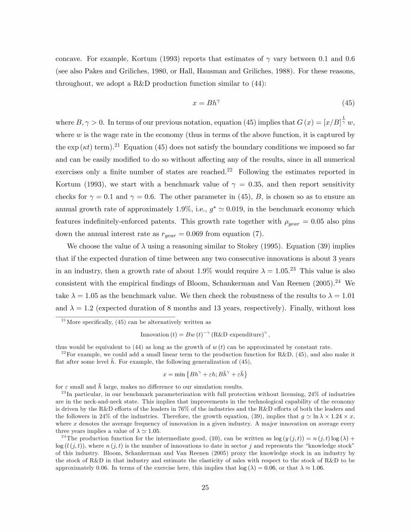
throughout, we adopt a R&D production function similar to (44):

x = Bhγ (45)

whereB, γ > 0. In terms of our previous notation, equation (45) implies thatG (x) = [x/B]1γ w,

where w is the wage rate in the economy (thus in terms of the above function, it is captured by

the exp (κt) term).21 Equation (45) does not satisfy the boundary conditions we imposed so far

and can be easily modified to do so without affecting any of the results, since in all numerical

exercises only a finite number of states are reached.22 Following the estimates reported in

Kortum (1993), we start with a benchmark value of γ = 0.35, and then report sensitivity

checks for γ = 0.1 and γ = 0.6. The other parameter in (45), B, is chosen so as to ensure an

annual growth rate of approximately 1.9%, i.e., g∗ ' 0.019, in the benchmark economy which

features indefinitely-enforced patents. This growth rate together with ρyear = 0.05 also pins

down the annual interest rate as ryear = 0.069 from equation (7).

We choose the value of λ using a reasoning similar to Stokey (1995). Equation (39) implies

that if the expected duration of time between any two consecutive innovations is about 3 years

in an industry, then a growth rate of about 1.9% would require λ = 1.05.23 This value is also

consistent with the empirical findings of Bloom, Schankerman and Van Reenen (2005).24 We

take λ = 1.05 as the benchmark value. We then check the robustness of the results to λ = 1.01

and λ = 1.2 (expected duration of 8 months and 13 years, respectively). Finally, without loss

21More specifically, (45) can be alternatively written as

Innovation (t) = Bw (t)−γ (R&D expenditure)γ ,

thus would be equivalent to (44) as long as the growth of w (t) can be approximated by constant rate.22For example, we could add a small linear term to the production function for R&D, (45), and also make it

flat after some level h. For example, the following generalization of (45),

x = min{Bhγ + εh;Bhγ + εh

}for ε small and h large, makes no difference to our simulation results.23 In particular, in our benchmark parameterization with full protection without licensing, 24% of industries

are in the neck-and-neck state. This implies that improvements in the technological capability of the economyis driven by the R&D efforts of the leaders in 76% of the industries and the R&D efforts of both the leaders andthe followers in 24% of the industries. Therefore, the growth equation, (39), implies that g ' lnλ × 1.24 × x,where x denotes the average frequency of innovation in a given industry. A major innovation on average everythree years implies a value of λ ' 1.05.24The production function for the intermediate good, (10), can be written as log (y (j, t)) = n (j, t) log (λ) +

log (l (j, t)), where n (j, t) is the number of innovations to date in sector j and represents the “knowledge stock”of this industry. Bloom, Schankerman and Van Reenen (2005) proxy the knowledge stock in an industry bythe stock of R&D in that industry and estimate the elasticity of sales with respect to the stock of R&D to beapproximately 0.06. In terms of the exercise here, this implies that log (λ) = 0.06, or that λ ≈ 1.06.

25

of generality, we normalize labor supply to 1. This completes the determination of all the

parameters in the model except the IPR policy.

As noted above, we begin with the full patent protection regime, i.e., η = {0, 0, ...}. Wethen move to a comparison of the optimal (welfare-maximizing) uniform IPR policy ηuni to

the optimal state-dependent IPR policy. Since it is computationally impossible to calculate

the optimal value of each ηn, we limit our investigation to a particular form of state-dependent

IPR policy, whereby the same η applies to all industries that have a technology gap of n = 5

or more. In other words, the IPR policy can be represented as:

IPR policy→Technology gap: n→

none−0

η1︷︸︸︷−1

η2︷︸︸︷−2

η3︷︸︸︷−3

η4︷︸︸︷−4

η5︷ ︸︸ ︷−5−6−7−8−9−10−11−.−.−∞

We checked and verified that allowing for further flexibility (e.g., allowing η5 and η6 to differ)

has little effect on our results.

The numerical methodology we pursue relies on uniformization and value function iteration.

The details of the uniformization technique are described in the proof of Lemma 1 in the

Appendix (for details of value function iteration, see Judd, 1999). In particular, we first take

the IPR policy η as given and make an initial guess for the equilibrium labor share ω∗. Then

for a given ω∗, we generate a sequence of values {vn}∞n=−∞, and we derive the optimal R&D

policies, {x∗n}∞n=−∞ and the steady-state distribution of industries, {µ∗n}

∞n=0. After convergence,

we compute the growth rate g∗ and welfare, and then check for market clearing in the labor

market from equation (23). Depending on whether there is excess demand for or supply

of labor, ω∗ is varied and the numerical procedure is repeated until the entire steady-state

equilibrium for a given IPR policy is computed. The process is then repeated for different IPR

policies.

In the state-dependent IPR case, the optimal (welfare-maximizing) IPR policy sequences,

η, are computed one element at a time, until we find the welfare-maximizing value for that

component, for example, η1. We then move the next component, for example, η2. Once the

welfare-maximizing value of η2 is determined, we go back to optimize over η1 again, and this

procedure is repeated recursively until convergence.25

6 Optimal IPR Policy

In this section, we present a quantitative analysis of our baseline model.25After we find a maximizer (η∗), we also evaluate several random policy combinations around the maximizer

to verify the solution.

26

6.1 Full IPR Protection

We start with the benchmark with full protection, which is the case that the existing literature

has considered so far (e.g., Aghion, Harris, Howitt and Vickers, 2001). In terms of our model,

this corresponds to ηn = 0 for all n. We choose the parameter B in terms of (45), so that the

benchmark economy has an annual growth rate of 1.86%.

[Figure 3 & 4 & 5 here]

The value function for this benchmark case is shown in Figure 3 (solid line). The value

function has decreasing differences for n ≥ 0, which is consistent with the results in Proposition

4, and features a constant level for all followers (since there is no state dependence in the IPR

policy). Figure 4 shows the level of R&D efforts for leaders and followers in this benchmark

(again solid line). Again consistent with Proposition 4, this figure also shows that the R&D

level of a leader declines as the technology gap increases and that the highest level of R&D

is for firms that are neck-and-neck (i.e., at the technology gap of n = 0). Since there is no

state-dependent IPR policy, all followers undertake the same level of R&D effort, which is also

shown in the figure.

Figure 5 shows the distribution of industries according to technology gaps (again the solid

line refers to the benchmark case). The mode of the distribution is at the technology gap of

n = 1, but there is also a significant concentration of industries at technology gap n = 0,

because innovations by the followers take them to the “neck-and-neck”state.

[Table 1 here]

The first column of Table 1 also reports the results for this benchmark simulation. As noted

above, in each case B is chosen such that the annual growth rate is equal to 0.0186, which

is recorded at the bottom of Table 1 together with the initial consumption and welfare levels

according to (42) and (43). The table also shows the R&D levels x∗0, x∗−1 and x

∗1 (0.35, 0.22 and

0.29), the frequencies of industries with technology gaps of 0, 1 and 2. The steady-state value of

ω is 0.95. Since labor is the only factor of production in the economy, ω∗ should not be thought

of as the labor share in GDP. Instead, 1− ω∗ measures the share of pure monopoly profits invalue added. In the benchmark parameterization, this corresponds to 5% of GDP, which is

reasonable.26 Finally, the table also shows that in this benchmark parameterization 3.2% of

26Bureau of Economic Analysis (2004) reports that the ratio of before-tax profits to GDP in the US economyin 2001 was 7% and the after-tax ratio was 5%.

27

the workforce is working as researchers, which is also consistent with US data.27 These results

are encouraging for our simple quantitative exercise, since with very few parameter choices,

the model generates reasonable numbers, especially for the share of the workforce allocated to

research.28

6.2 Optimal Uniform IPR Protection

For reference, we now characterize optimal uniform IPR policy, that is, we impose that ηn = η

for all n, and look for values of η that maximizes the welfare in the economy. Column 2 of

Table 1 shows that the welfare-maximizing value of η is not different from zero at the three-digit

level. Therefore the results of the full protection case carries over to uniform policy as well.

The main reason for this result is the quick catch-up assumption. Recall that the uniform IPR

policy discourages innovation, but generates a potential benefit because of the composition

effect (bringing more firms into neck-and-neck position). In the quick catch-up regime, firms

come into neck-and-neck position at a Poisson rate of 0.22, which results in 35% of sectors

being in state 0 and 77% at two-step gap or below. This implies that there are only limited

composition gains. In this light, it is not surprising that relaxing the IPR protection uniformly

is not beneficial; it generates a significant disincentive effect and little benefit. Therefore,

optimal IPR policy is to set full protection, η∗ = 0, and thus the value functions, innovation

rates and industry distributions under optimal uniform IPR policy are given by the solid lines

in Figures 3-5.

6.3 Optimal State-Dependent IPR

We next turn to our major question; whether state-dependent IPR makes a significant differ-

ence relative to the uniform IPR. In particular, we look for the combination of {η1, ..., η5} thatmaximizes the welfare. The new value function, innovation rates and industry distribution are

plotted in Figure 3-5 and the numerical results are shown in column 3 of Table 1.

Two features are worth noting. First, the growth rate increases noticeably relative to

column 1; it is now 2.04% instead of 1.86%. Second and more important, we see the key pattern

that will be present in all of our quantitative results: optimal state-dependent policy {η1, ..., η5}27According to National Science Foundation (2006), the ratio of scientists and engineers in the US workforce

in 2001 is about 4%.28Most endogenous growth models imply that a significantly greater fraction of the labor force should be

employed in the research sector and one needs to introduce various additional factors to reduce the profitabilityof research or to make entry into research more diffi cult. In the current model, the step-by-step nature ofinnovation and competition plays this role and generates a plausible allocation of workers between research andproduction.

28

provides greater protection to technology leaders that are further ahead. In particular, we find

that the optimal policy involves η1 = 0.71, η2 = 0.08, and η3 = η4 = η5 = 0. This corresponds

to very little patent protection for firms that are one step ahead of the followers. In particular,

since η1 = 0.71 and x∗−1 = 0.12, in this equilibrium firms that are one step behind followers are

more than six times as likely to catch up with the technology leader because of the expiration

of the patent of the leader as they are likely to catch up because of their own successful R&D.

Then, there is a steep increase in the protection provided to technology leaders that are two

steps ahead, and η2 is 1/12th of η1. Perhaps even more remarkably, after a technology gap of

three or more steps, optimal IPR involves full protection, and patents never expire.

This pattern of greater protection for technology leaders that are further ahead may go

against a naïve intuition that state-dependent IPR policy should try to boost the growth rate

of the economy by bringing the industries with largest technology gaps (where leaders engage in

little R&D) into neck-and-neck competition. This composition effect is present, but dominated

by another, more powerful force, the trickle-down effect. The intuition for the trickle-down

effect is as follows: by providing secure patent protection to firms that are three or more steps

ahead of their rivals, optimal state-dependent IPR increases the R&D effort of leaders that are

one and two steps ahead as well. This is because technology leaders that are only one or two

steps ahead now face greater returns to R&D, which will not only increase their profits but

also the security of their intellectual property. Mechanically, high levels of η1 and η2 reduce

v1 and v2, while high IPR protection for more advanced firms increases vn for n ≥ 3, and this

increases the R&D incentives of leaders at n = 1 or at n = 2.29

Providing more secure patent protection through less frequent catch-up benefits an n-step

leader more than (n+ 1)-step leader since the preserved profit is higher for a more advanced

firm. This results in a steeper value function as illustrated in Figure 3. The slope of the value

function is the key determining factor for R&D decisions and this increase in slope reflects

itself in overall higher R&D effort by the leaders in Figure 4. It is also notable that state-

dependent IPR introduces positive incentive effect while gaining also from the composition.

Figure 5 shows that the mode of the new distribution is at n = 0. The average innovation rate

is higher (as reflected on a higher growth rate, g = 2.04%) and the average mark-up is lower

(C (0) increases by 52%). This pattern of greater R&D investments under state-dependent

29An alternative intuition, suggested by an anonymous referee, is that when the technology gap is greater,leaders will lose more from a relaxation of IPR. However, this intuition can only be partial, since, as shown inSection 2, state-dependent relaxation of IPR in this form creates a positive incentive effect, which is central toour results (and this is independent of how much technology leaders lose as a result of the relaxation of IPR).As a result, we believe that the trickle-down of incentives is the more correct intuition for our results.

29

IPR contrasts with uniform IPR, which always reduces R&D of all firms. The possibility that

imperfect state-dependent IPR protection can increase (rather than reduce) R&D incentives

is a novel feature of our approach and has also been shown explicitly in the partial equilibrium

model of Section 2.

6.4 Robustness

The patterns shown in Figures 3-5 and Table 1 are highly robust. In the working paper version,

we repeated this entire exercise for various combinations of values of γ and λ (in particular,

varying γ to γ = 0.1 and γ = 0.6, and λ to λ = 1.01 and λ = 1.2). The overall pattern and

in fact the quantitative magnitudes are remarkably similar to the baseline reported here. We

do not report these robustness checks to save space (they are available upon request); instead,

we focus on the results in the slow catch-up regime.

7 Optimal IPR Policy in the Slow Catch-up Regime

In this section, we extend our analysis to an environment where followers close the gap with

technology leaders also step by step. This environment will further allow us to introduce

different types of R&D efforts by followers and study several different dimensions of IPR

policy.

7.1 Value Functions

The environment is the same as in Section 3, except that we now assume that successful R&D

by followers close is the gap between themselves and the technology leader by one step. We

will allow for different types of R&D below. The equivalent expressions for the value functions

(29)-(31) in this case are

ρvn = maxxn≥0

{(1− λ−n

)− ω∗G (xn) + xn [vn+1 − vn] + x∗−n [vn−1 − vn] + ηn [v0 − vn]

}for n ∈ N,

(46)

ρv0 = maxx0≥0

{−ω∗G (x0) + x0 [v1 − v0] + x∗0 [v−1 − v0]} , (47)

and

ρv−n = maxx−n≥0

{−ω∗G (x−n) + x−n [v−n+1 − v−n] + x∗n [v−n−1 − v−n] + ηn [v0 − v−n]} for n ∈ N.(48)

These expressions are intuitive in light of those presented in Section 3, in particular, (29)-

(31). The only difference from equations (29)-(31) is that, when a follower innovates, an

30

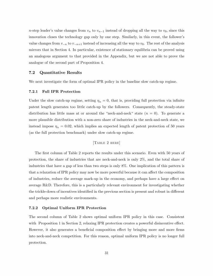
n-step leader’s value changes from vn to vn−1 instead of dropping all the way to v0, since this

innovation closes the technology gap only by one step. Similarly, in this event, the follower’s

value changes from v−n to v−n+1 instead of increasing all the way to v0. The rest of the analysis

mirrors that in Section 4. In particular, existence of stationary equilibria can be proved using

an analogous argument to that provided in the Appendix, but we are not able to prove the

analogue of the second part of Proposition 4.

7.2 Quantitative Results

We next investigate the form of optimal IPR policy in the baseline slow catch-up regime.

7.2.1 Full IPR Protection

Under the slow catch-up regime, setting ηn = 0, that is, providing full protection via infinite

patent length generates too little catch-up by the followers. Consequently, the steady-state

distribution has little mass at or around the “neck-and-neck“ state (n = 0). To generate a

more plausible distribution with a non-zero share of industries in the neck-and-neck state, we

instead impose ηn = 0.02, which implies an expected length of patent protection of 50 years

(as the full protection benchmark) under slow catch-up regime.

[Table 2 here]

The first column of Table 2 reports the results under this scenario. Even with 50 years of

protection, the share of industries that are neck-and-neck is only 2%, and the total share of

industries that have a gap of less than two steps is only 8%. One implication of this pattern is

that a relaxation of IPR policy may now be more powerful because it can affect the composition

of industries, reduce the average mark-up in the economy, and perhaps have a large effect on

average R&D. Therefore, this is a particularly relevant environment for investigating whether

the trickle-down of incentives identified in the previous section is present and robust in different

and perhaps more realistic environments.

7.2.2 Optimal Uniform IPR Protection

The second column of Table 2 shows optimal uniform IPR policy in this case. Consistent

with Proposition 1 in Section 2, relaxing IPR protection creates a powerful disincentive effect.

However, it also generates a beneficial composition effect by bringing more and more firms

into neck-and-neck competition. For this reason, optimal uniform IPR policy is no longer full

protection.

31

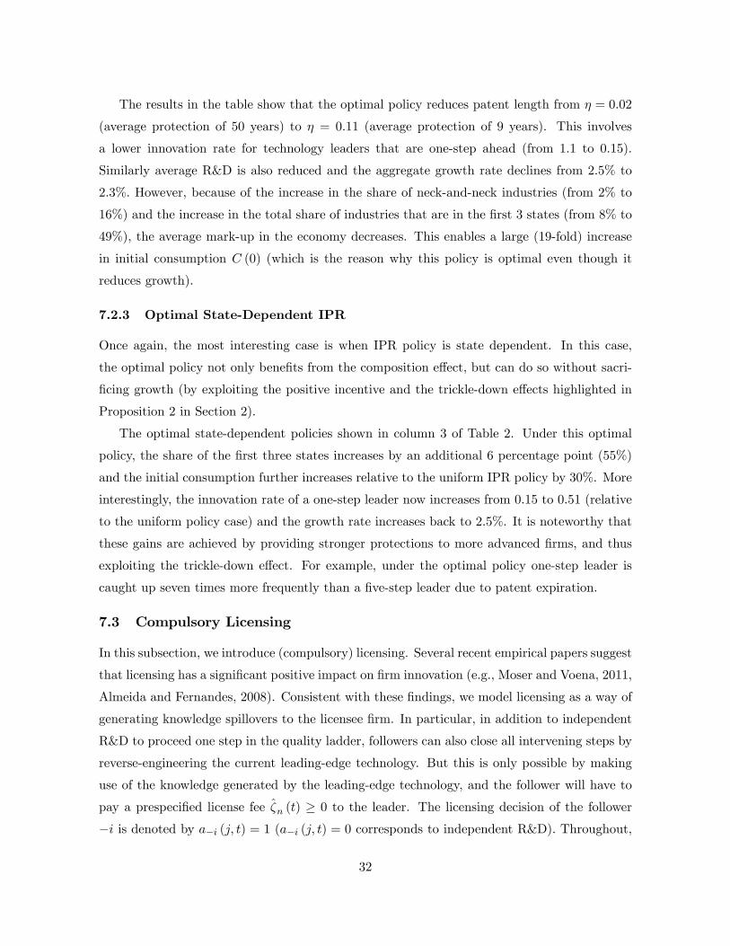
The results in the table show that the optimal policy reduces patent length from η = 0.02

(average protection of 50 years) to η = 0.11 (average protection of 9 years). This involves

a lower innovation rate for technology leaders that are one-step ahead (from 1.1 to 0.15).

Similarly average R&D is also reduced and the aggregate growth rate declines from 2.5% to

2.3%. However, because of the increase in the share of neck-and-neck industries (from 2% to

16%) and the increase in the total share of industries that are in the first 3 states (from 8% to

49%), the average mark-up in the economy decreases. This enables a large (19-fold) increase

in initial consumption C (0) (which is the reason why this policy is optimal even though it

reduces growth).

7.2.3 Optimal State-Dependent IPR

Once again, the most interesting case is when IPR policy is state dependent. In this case,

the optimal policy not only benefits from the composition effect, but can do so without sacri-

ficing growth (by exploiting the positive incentive and the trickle-down effects highlighted in

Proposition 2 in Section 2).

The optimal state-dependent policies shown in column 3 of Table 2. Under this optimal

policy, the share of the first three states increases by an additional 6 percentage point (55%)

and the initial consumption further increases relative to the uniform IPR policy by 30%. More

interestingly, the innovation rate of a one-step leader now increases from 0.15 to 0.51 (relative

to the uniform policy case) and the growth rate increases back to 2.5%. It is noteworthy that

these gains are achieved by providing stronger protections to more advanced firms, and thus

exploiting the trickle-down effect. For example, under the optimal policy one-step leader is

caught up seven times more frequently than a five-step leader due to patent expiration.

7.3 Compulsory Licensing

In this subsection, we introduce (compulsory) licensing. Several recent empirical papers suggest

that licensing has a significant positive impact on firm innovation (e.g., Moser and Voena, 2011,

Almeida and Fernandes, 2008). Consistent with these findings, we model licensing as a way of

generating knowledge spillovers to the licensee firm. In particular, in addition to independent

R&D to proceed one step in the quality ladder, followers can also close all intervening steps by

reverse-engineering the current leading-edge technology. But this is only possible by making

use of the knowledge generated by the leading-edge technology, and the follower will have to

pay a prespecified license fee ζn (t) ≥ 0 to the leader. The licensing decision of the follower

−i is denoted by a−i (j, t) = 1 (a−i (j, t) = 0 corresponds to independent R&D). Throughout,

32

we allow a−i (j, t) ∈ [0, 1] for mathematical convenience. The fees in question are compulsory

license fees imposed by policy and are state-dependent, and thus we represent them as:

ζ (t) : N→ R+ ∪ {+∞} .

Note that ζ (t)≡{ζ1 (t) , ζ2 (t) , ...

}is a function of time. This is natural, since in a growing

economy, license fees should not remain constant. As in (28), in what follows we assume that

license fees are also scaled up by GDP, so that ζn ≡ ζn (t) /Y (t), to keep the equilibrium

stationary. We discuss voluntary licensing below.

7.3.1 Value Functions with Compulsory Licensing

With a similar reasoning to before, relevant value functions in this case can be written as

ρvn = maxxn≥0

{ (1− λ−n

)− ω∗G (xn) + xn [vn+1 − vn]

+a∗−nx∗−n [v0 − vn + ζn] +

(1− a∗−n

)x∗−n [vn−1 − vn] + ηn [v0 − vn]

}for n ∈ N,

where a∗−n is the equilibrium value of licensing decision by a follower that is n steps behind, and

ζn is the license fee that it has to pay. The value for neck-and-neck firms remain unchanged

while the values for followers becomes

ρv−n = maxx−n≥0,a−n∈[0,1]

{−ω∗G (x−n) + a−nx−n [v0 − v−n − ζn]

+ (1− a−n)x−n [v−n+1 − v−n] + x∗n [v−n−1 − v−n] + ηn [v0 − v−n]

}for n ∈ N,

Note that licensing a−n ∈ [0, 1] is the new additional decision variable of the follower.

Full IPR protection in this case corresponds to prohibitively high licensing fees, i.e., ζn =∞for all n, and as in the previous subsection, patent protection has expected duration of 50

years (η = 0.02). Therefore, the results in this case will be identical to those reported for full

protection in the previous subsection (column 1 of Table 2). This is indeed the case; these

results are repeated in column 1 of Table 3 for ease of comparison with the remaining results

in this table.

[Table 3 here]

7.3.2 Optimal Uniform IPR Protection

Uniform compulsory licensing policy now corresponds to ζn = ζ∗ ≥ 0. The results under the

optimal choice of such uniform compulsory licensing policy are reported in the second column

of Table 3. This optimal policy involves ζ∗ = 1.61, which is more than half of the surplus that

a three-step follower generates from licensing, v0 − v−3 = 2.9.

33

Since this type of licensing allows for more frequent catch-up by followers, a greater share

of industries are now in tight competition. In particular, the total share of industries with

one or two step gaps goes up to 66% (this number was 8% under full protection). This

again corresponds to a powerful composition effect and generates a significant reduction in the

average mark-up and a corresponding increase in initial consumption. However, consistent with

our previous results, this type of uniform licensing again generates a significant disincentive

effect on technology leaders. In particular, more frequent catch-up implies a shorter durations

of positive profits. As a result, innovation incentives are reduced; the innovation rate of a

one-step leader is now 0.43 instead of 1.1 and the average growth rate declines from 2.5% to

2.1%.

7.3.3 Optimal State-Dependent IPR

As in our previous exercises, the negative incentive effects of uniform relaxations of IPR pro-

tection are rectified when policy is state dependent. Optimal state-dependent policy has in

fact qualitatively very similar pattern to those reported above. Most importantly, column 3 of

Table 3 shows that optimal state-dependent policy provides greater protection to technology

leaders that are more advanced. For example, while a two-step leader receives a license fee of

ζ∗2 = 1.5, a five-step leader receives more than its double, ζ∗5 = 3.3. Given this pattern, the

trickle-down effect is again at work and generates positive innovation incentives: the innova-

tion rate of a one-step leader increases to x∗1 = 0.46 and the aggregate growth rate goes back

to 2.5% from 2.1%. This positive gain is generated without sacrificing the composition effect.

Under this policy, 50% of total industries operate with a technology gap less than two and the

initial consumption C (0) is now even higher than under uniform policy (by 40%).

7.3.4 Compulsory Versus Bargained License Fees

The analysis so far has characterized the steady-state equilibrium for a given sequence of li-

cense fees ζ, implicitly assumed to be determined by IPR policy– i.e., these fees correspond

to compulsory licensing fees for intellectual property that has been patented. This, therefore,

corresponds to a world in which once a company patents an innovation, the knowledge embed-

ded in this innovation can be used by its competitors as long as they pay a prespecified license

fee.

One may also wish to consider an alternative world in which license fees are determined by

bilateral bargaining. To characterize the equilibrium in such a world, one must first conduct

exactly the same analysis as we have done in this subsection. In other words, one must

34

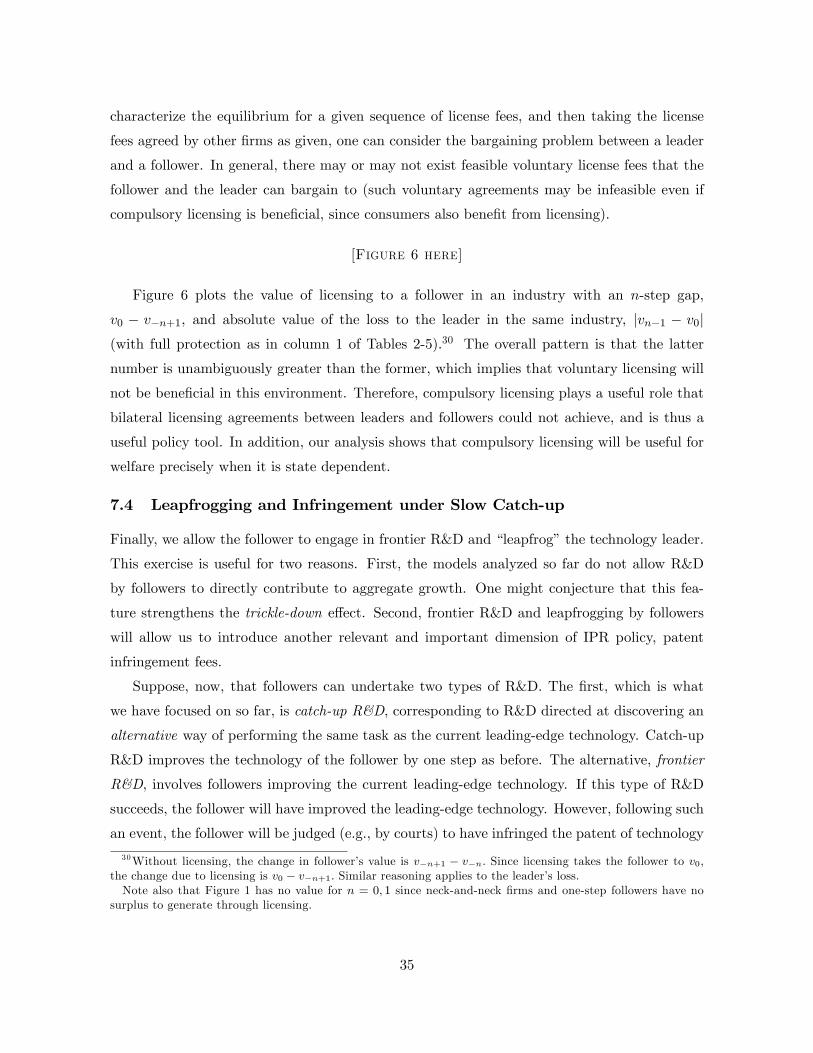
characterize the equilibrium for a given sequence of license fees, and then taking the license

fees agreed by other firms as given, one can consider the bargaining problem between a leader

and a follower. In general, there may or may not exist feasible voluntary license fees that the

follower and the leader can bargain to (such voluntary agreements may be infeasible even if

compulsory licensing is beneficial, since consumers also benefit from licensing).

[Figure 6 here]

Figure 6 plots the value of licensing to a follower in an industry with an n-step gap,

v0 − v−n+1, and absolute value of the loss to the leader in the same industry, |vn−1 − v0|(with full protection as in column 1 of Tables 2-5).30 The overall pattern is that the latter

number is unambiguously greater than the former, which implies that voluntary licensing will

not be beneficial in this environment. Therefore, compulsory licensing plays a useful role that

bilateral licensing agreements between leaders and followers could not achieve, and is thus a

useful policy tool. In addition, our analysis shows that compulsory licensing will be useful for

welfare precisely when it is state dependent.

7.4 Leapfrogging and Infringement under Slow Catch-up

Finally, we allow the follower to engage in frontier R&D and “leapfrog”the technology leader.

This exercise is useful for two reasons. First, the models analyzed so far do not allow R&D

by followers to directly contribute to aggregate growth. One might conjecture that this fea-

ture strengthens the trickle-down effect. Second, frontier R&D and leapfrogging by followers

will allow us to introduce another relevant and important dimension of IPR policy, patent

infringement fees.

Suppose, now, that followers can undertake two types of R&D. The first, which is what

we have focused on so far, is catch-up R&D, corresponding to R&D directed at discovering an

alternative way of performing the same task as the current leading-edge technology. Catch-up

R&D improves the technology of the follower by one step as before. The alternative, frontier

R&D, involves followers improving the current leading-edge technology. If this type of R&D

succeeds, the follower will have improved the leading-edge technology. However, following such

an event, the follower will be judged (e.g., by courts) to have infringed the patent of technology

30Without licensing, the change in follower’s value is v−n+1 − v−n. Since licensing takes the follower to v0,the change due to licensing is v0 − v−n+1. Similar reasoning applies to the leader’s loss.Note also that Figure 1 has no value for n = 0, 1 since neck-and-neck firms and one-step followers have no

surplus to generate through licensing.

35

leader with probability τ ∈ (0, 1) and will be required to pay a prespecified infringement penalty

(fee) ϑn ≥ 0 to the leader. The infringement fees are also state dependent and represented by:

ϑ (t) : N→ R+ ∪ {+∞} ,

and we again adopt the normalization ϑn ≡ ϑn (t) /Y (t), and denote the Poisson arrival rate

of innovation by catch-up R&D and frontier R&D by xcn and xfn, respectively. Then the new

value of an n-step leader takes the following form:

ρvn = maxxn≥0

{ (1− λ−n

)− ω∗G (xn) + xn [vn+1 − vn]

+xc∗−n [vn−1 − vn] + xf∗−n [v−1 − vn + τϑn] + ηn [v0 − vn]

}for n ∈ N,

The main difference in this equation is that the follower has two different arrival rates of

innovation. If the follower is successful with frontier R&D, the current leader falls one step

behind the follower. However, in this event, with probability τ , it receives an infringement fee

of ϑn. With a similar reasoning, the value of an n-step follower now becomes:

ρv−n = maxxc−n≥0,xf−n≥0

{−ω∗G (x−n) + xc−n [v−n+1 − v−n] + xf−n [v1 − v−n − τϑn]

+x∗n [v−n−1 − v−n] + ηn [v0 − v−n]

}for n ∈ N.

The value of a neck-and-neck firm is unchanged.

The quantitative analysis requires an empirical estimate for τ . Lanjouw and Schankerman

(2001) report that around 10% of the US utility patents are filed for infringement. We therefore

set τ = 0.1.

Note also that since the followers now improve the technology frontier through frontier

R&D, the aggregate growth rate becomes

g∗ = lnλ

[2µ∗0x

∗0 +

∞∑n=1

µ∗n

(x∗n + xf∗−n

)]. (49)

Full protection in this case corresponds to infinite patent infringement fees, i.e., ϑn = ∞,and given the same parameter choices as before, will be identical to column 1 of Table 2. We

repeat these results in column 1 of Table 4 for ease of comparison with the rest of the table.

[Table 4 here]

7.4.1 Optimal Uniform IPR Protection

In the uniform policy case, we set ϑn = ϑ ≥ 0. Column 2 of Table 4 shows that the optimal

uniform policy in this case is ϑ∗ = 14. Recall that when a follower undertakes frontier inno-

vation, the probability the that it will have to make this payment is τ = 0.1. Therefore the

36

expected infringement payment is τ × ϑ∗ = 1.4 which is more than half of the surplus that a

three-step follower generates out of leapfrogging, v1 − v−3 = 2.7.

Column 2 also shows that under this policy, followers undertake more frontier R&D (x∗f−1 =

0.23) than catch-up R&D(x∗c−1 = 0.15

). Parallel to the previous uniform policies, the shorter

duration of monopoly position resulting from innovation reduces innovation incentives. For

example, one-step leaders now innovate at the rate 0.3 instead of 1.1. However, despite this

disincentive effect, the growth rate increases slightly because leapfrogging allows followers to

directly contribute to aggregate growth, as shown by equation (49).

Column 2 also shows that the share of industries in one-step gap is now much larger,

µ1 = 0.42. This is because leapfrogging puts the follower one-step ahead of the previous

leader. Thanks to this effect, optimal uniform IPR protection achieves lower average mark-up

and higher initial consumption as well as higher growth.

7.4.2 Optimal State-Dependent IPR

State-dependent IPR policy once again exploits the trickle-down effect and creates positive

incentive effects on innovation. The form of state-dependent policy is the same as before:

technologically more advanced leaders receive more protection in the form of higher fees when

followers infringe their patents. While a two-step leader receives ϑ∗1 = 18.1 in case of in-

fringement, a five-step leader receives more than double of this fee, ϑ∗5 = 43.7. In expectation,

a three-step follower pays almost 3/4th of the surplus that it generates from leapfrogging

(τ × ϑ∗3 = 3.1 versus v1 − v−3 = 4.1). As a result of this pattern, state-dependent policy not

only generates a greater welfare gain in terms of the initial consumption (C (0) is now approx-

imately twice the level under the optimal uniform policy), but it also exploits the trickle-down

effect and increases the equilibrium growth rate by an additional 0.5 percentage point relative

to the uniform policy.

7.5 Patent Length, Compulsory Licensing and Infringements Fees underSlow Catch-up

In this subsection, we investigate the slow catch-up environment when all three IPR policies

are simultaneously present. We do not repeat the value functions to save space.

[Table 5 here]

Table 5 first shows our benchmark full protection economy in the first column. The second

and third columns report the optimal uniform and state-dependent policies with all three types

37

of policies present. The results are very similar to those reported in subsection 7.4 (with only

leapfrogging), except that the patent lengths are now set to infinity (ηn = 0). The optimal

IPR policy in this case involves infinitely long patents with prohibitively high compulsory

license fees. The only dimension in which IPR protection is not full is because of moderate

infringement fees, which permit followers to undertake frontier R&D and leapfrog technology

leaders.

Most importantly for our focus, column 3 again shows the benefits of state-dependent IPR

policy. This policy again provides greater protection for technology leaders and exploits the

trickle-down effect. As a result, initial consumption is approximately twice the level under

uniform IPR and innovation incentives are stronger, and the long-run growth rate increases

from 2.5% to 3.3%.

7.6 Robustness Checks

Table 6 shows that the patterns documented in Table 5, particularly the gains from state-

dependent policy and the major role played by the trickle-down effect, are robust for reasonable

changes in parameter values.

[Table 6 here]

In this table, in each column we change one of the two parameters λ and γ (increasing or

reducing λ to 1.2 or 1.01, and increasing or reducing γ to 0.6 or 0.1). In each case, we also

change the parameter B in equation (45) to ensure the growth rate of the benchmark economy

with full IPR protection is the same as in our initial baseline economy, g∗ = 1.86%.

To save space, we only show the results from the optimal state-dependent policies. Table 6

shows that the qualitative patterns in Table 5 are relatively robust. In all cases, optimal state-

dependent IPR is shaped by the trickle-down effect. In all of the various parameterizations we

have considered (and with different combinations of policies), there is little protection provided

to technology leaders that are one-step ahead, but IPR protection grows as the technology gap

increases. This is the typical pattern implied by the trickle-down effect. In addition, in all

cases when all three forms of policy are incorporated, optimal IPR policy provides patents

of infinite duration and prohibitively high compulsory licensing fees, but deviates from full

IPR protection by imposing moderate levels of infringement fees. Most importantly for us,

in all cases, these infringements fees are state dependent and provide greater protection to

technologically more advanced leaders.

38

8 Conclusions

In this paper, we emphasized the importance of dynamic interactions between IPR protec-

tion and competition for understanding the structure of optimal IPR policy. Our main result

highlights the importance of a new and powerful effect, the trickle-down effect, which implies

that protection given to companies with significant technological leads over their rivals also

dynamically incentivizes companies with more limited technological leads– as further innova-

tion will not only increase their productivity but also grant them additional IPR protection.

This new effect implies that optimal IPR policy should be state-dependent and provide greater

protection to companies with significant technological leads and only limited IPR protection

for those without.

To systematically investigate these issues, we developed a dynamic general equilibrium

framework with cumulative (step-by-step) innovations. In each industry, technology leaders

innovate in order to widen the gap between themselves and the followers, which enables them

to charge higher markups. Followers innovate to catch up with or surpass the technology

leaders in their industry (by undertaking “frontier R&D”), and can also license the technology

of leaders. IPR policy regulates the length of patents, whether licensing is possible and the

size of patent infringement fees.

We provided existence and characterization results, and a quantitative analysis of the form

of “optimal” (welfare-maximizing) IPR policy. In several different environments and under

different parameter values, we consistently found that the trickle-down effect is present and

powerful. It implies that optimal IPR should be state-dependent and should provide greater

protection to firms with greater technological lead over their rivals. In our benchmark para-

meterization, for example, optimal IPR policy increases the growth rate of the economy from

1.86% to 2.04%, and does so while also significantly increasing initial consumption (and in

fact reducing the overall amount of resources allocated to the R&D sector). We also showed

that similar qualitative and quantitative results are obtained when followers catch up with

technology leaders only slowly. In this extended environment, we also investigated the form of

optimal compulsory licensing fees and patent infringement fees, and found them to be similarly

state-dependent (in a way that provides greater protection to firms that are technologically

more advanced relative to their rivals). These extensions further showed that compulsory li-

censing, which allows followers to build on the leading-edge technology in return of a license

fee, also has a major impact on the equilibrium growth rate.

Our main results go against a naïve intuition that providing less protection to techno-

39

logically more advanced firms is socially beneficial because it would exploit a composition

effect (bringing firms that are furthest apart into “neck and neck”competition to both reduce

markups and increase R&D which results from tight competition). This naïve intuition is not

correct precisely because of the trickle-down effect we emphasized above. The trickle-down

effect implies that providing greater protection to suffi ciently advanced technology leaders not

only increases their R&D efforts but also raises the R&D efforts of all technology leaders that

are less advanced than this level. This is because the reward to innovation now includes the

greater protection that they will receive once they reach this higher level of technology. Our

analysis and results suggest that in addition to the reasoning based on the static trade-off

between IPR protection and competition, the trickle-down effect should also be factored into

policy analysis, and naturally calls for future empirical work to estimate its empirical magni-

tude.

In this context, it should be emphasized that our objective in this paper has not been to

derive practical policy prescriptions. There is little doubt that our model is simplified, excludes

a whole host of important factors, and ignores potential limitations on the form and complexity

of IPR policies. Nevertheless, we believe that our results demonstrate a range of robust and

new effects that should be further investigated in future work.

More generally, the analysis in this paper suggests that a move to a richer menu of IPR

policies, in particular, a move towards optimal state-dependent policies, may significantly

increase innovation, economic growth and welfare. The results also show that the form of

optimal IPR policy may depend on the industry structure (and the technology of catch-up

within the industry). The next step in this line of research should be to investigate the

robustness of these effects in different models of industry dynamics. It would also be useful to

study whether the relationship between the form of optimal IPR policy and industry structure

suggested by our analysis also applies when variation in industry structure has other sources

(for example, differences in the extent of fixed costs or demand structure causing differential

gaps between technology leaders and followers across industries). The most important area for

future work is a detailed empirical investigation of the form of optimal IPR policy, using both

better estimates of the effects of IPR policy on innovation rates and also structural models

that would enable the evaluation of the effects of different policies on equilibrium growth and

welfare.

40

Appendix: Proofs

Derivation of Optimal R&D Decisions in the Partial Equilibrium Model

Since the costs are linear, optimal R&D decisions imposed that, in equilibrium,

vn+1 − vn = φ, for each n ∈ {−2,−1, 0, 1} . (50)

Combining this result with equation (1) gives the value of a two-step follower is

v−2 =π−2 + 2φη2

r.

The previous equation, together with (50) implies

vn = v−2 + φ (n+ 2) =π−2 + 2φη2

r+ φ (n+ 2) , for each n ∈ {−1, 0, 1, 2} . (51)

Now we can use the value of v2 to solve for x∗−2 from equation (1) . Similarly, combining (51) with (2)gives the value of x∗−1; (51) with (3) gives x∗0. Finally, combining (51) with (4) gives the equilibriumvalue of x∗1. �

Derivation of Equation (27)

Fix the equilibrium R&D policies of other firms, x∗−n (t), the equilibrium interest and wage rates, r∗ (t)and w∗ (t), and equilibrium profits {Π∗n (t)}∞n=1. Then the value of the firm that is n steps ahead attime t can be written as:

Vn (t) = maxxn(t)

{[Π∗n (t)− w∗ (t)G (xn (t))] ∆t + o (∆t) (52)

+ exp (−r∗ (t+ ∆t) ∆t)

(xn (t) ∆t+ o (∆t))Vn+1 (t+ ∆t)

+(ηn∆t+ x∗−n (t) ∆t+ o (∆t)

)V0 (t+ ∆t)

+(1− xn (t) ∆t− ηn∆t− x∗−n (t) ∆t− o (∆t)

)Vn (t+ ∆t)

.

The first part of this expression is the flow profits minus R&D expenditures during a time intervalof length ∆t. The second part is the continuation value after this interval has elapsed. Vn+1 (t) andV0 (t) are defined as net present discounted values for a leader that is n + 1 steps ahead and a firmin an industry that is neck-and-neck (i.e., n = 0). The second part of the expression uses the factthat in a short time interval ∆t, the probability of innovation by the leader is xn (t) ∆t+ o (∆t), whereo (∆t) again denotes second-order terms. This explains the first line of the continuation value. For theremainder of the continuation value, note that the probability that the follower will catch up with theleader is

[ηn + x∗−n (t)

]∆t+ o (∆t). Finally, the last line applies when no R&D effort is successful and

patents continue to be enforced, so that the technology gap remains at n steps. Now, subtract Vn (t)from both sides, divide everything by ∆t, and take the limit as ∆t→ 0 to obtain (27). �

Proof of Proposition 3

Equations (24) and (26) imply

Y (t) =w (t)

ω (t)=Q (t)λ−

∑∞n=0 nµ

∗n(t)

ω (t).

41

Since ω (t) = ω∗ and {µ∗n}∞n=0 are constant in steady state, Y (t) grows at the same rate as Q (t).

Therefore,

g∗ = lim∆t→0

lnQ (t+ ∆t)− lnQ (t)

∆t.

Now note the following: during an interval of length ∆t (i) in the fraction µ∗n of the industries withtechnology gap n ≥ 1 the leaders innovate at a rate x∗n∆t+o (∆t); (ii) in the fraction µ∗0 of the industrieswith technology gap of n = 0, both firms innovate, so that the total innovation rate is 2x∗0∆t+ o (∆t));and (iii) each innovation increase productivity by a factor λ. Combining these observations, we have

lnQ (t+ ∆t) = lnQ (t) + lnλ

[2µ∗0x

∗0∆t+

∞∑n=1

µ∗nx∗n∆t+ o (∆t)

].

Subtracting lnQ (t), dividing by ∆t and taking the limit ∆t→ 0 gives (39). �

Proof of Proposition 4

We prove this proposition in four parts. (1) Existence of a steady-state equilibrium. (2) Properties ofthe sequence of value functions. (3) Properties of the sequence of R&D decisions. (4) Uniqueness of aninvariant distribution given R&D policies.

Part 1: Existence of a Steady-State Equilibrium.First, note that each xn belongs to a compact interval [0, x], where x is the maximal flow rate of

innovation defined in (16) above. Now fix a labor share ω ∈ [0, 1] and a sequence 〈x〉 of (Markovian)steady-state strategies for all other firms in the economy, and consider the dynamic optimization problemof a single firm. Our first result characterizes this problem and shows that given some z ≡〈ω, x〉, thevalue function of an individual firm is uniquely determined, while its optimal R&D choices are givenby a convex-valued correspondence. In what follows, we denote sets and correspondences by uppercaseletters and refer to their elements by lowercase letters, e.g., xn (z) ∈ Xn [z].

Lemma 1 Consider a uniform IPR policy ηuni, and suppose that the labor share and the R&D policiesof all other firms are given by z = 〈ω, x〉. Then the dynamic optimization problem of an individual firmleads to a unique value function v [z] : {−1} ∪ Z+ → R+ and optimal R&D policy X [z] : {−1} ∪ Z+ ⇒[0, x] is compact and convex-valued for each z ∈ Z and upper hemi-continuous in z (where v [z] ≡{vn [z]}∞n=−1 and X [z] ≡

{Xn [z]

}∞n=−1

).

Proof. Fix z =⟨ω, {xn}∞n=−1

⟩, and consider the optimization problem of a representative firm,

written recursively as:

ρvn= maxxn∈[0,x]

{(1− λ−n

)− ωG (xn) + xn [vn+1 − vn] + x−1 [v0 − vn] + η [v0 − vn]} for n ∈ N

ρv0 = maxx0∈[0,x]

{−ωG (x0) + x0 [v1 − v0] + x0 [v−1 − v0]}

ρv−1 = maxx−1∈[0,x]

{−ωG (x0) + x−1 [v0 − v−1] + η [v0 − v−1]}.

We now transform this dynamic optimization problem into a form that can be represented as a con-traction mapping using the method of “uniformization”(see, for example, Ross, 1996, Chapter 5). Let

ξ = {xn}∞n=−1 and pn,n′(ξ | ξ

)be the probability that the next state will be n′ starting with state n

when the firm in question chooses policies ξ ≡{xn}∞n=−1 and the R&D policy of other firms is givenby ξ. Using the fact that, because of uniform IPR policy, x−n = x−1 for all n ∈ N, these transition

42

probabilities can be written as:

p−1,0

(ξ | ξ

)= x−1+η

xn+x−1+η pn,0

(ξ | ξ

)= x−1+η

xn+x−1+η

p0,−1

(ξ | ξ

)= x0

x0+x0pn,n+1

(ξ | ξ

)= xn

xn+x−1+η

p0,1

(ξ | ξ

)= x0

x0+x0

.

Uniformization involves adding fictitious transitions from a state into itself, which do not change thevalue of the program, but allow us to represent the optimization problem as a contraction. For thispurpose, define the transition rates ψn as

ψn

(ξ | ξ

)=

xn + x−1 + η for n ∈ {1, 2, ...}x−1 + η for n = −12xn for n = 0

.

These transition rates are finite since ψn(ξ | ξ

)≤ ψ ≡ 2x + η < ∞ for all n, where x is the maximal

flow rate of innovation defined in (16) in the text (both x and η are finite by assumption).Now following equation (5.8.3) in Ross (1996), we can use these transition rates and define the new

transition probabilities (including the fictitious transitions from a state to itself) as:

pn,n′(ξ | ξ

)=

ψn(ξ|ξ)

ψ pn,n′(ξ | ξ

)if n 6= n′

1− ψn(ξ|ξ)ψ if n = n′

.

This yields equivalent transition probabilities

p−1,−1

(ξ | ξ

)= 1− x−1+η

2x+η p−1,0

(ξ | ξ

)= x−1+η

2x+η p0,1

(ξ | ξ

)= x0

2x+η

p0,−1

(ξ | ξ

)= x0

2x+η p0,0

(ξ | ξ

)= 1− x0+x0

2x+η pn,n+1

(ξ | ξ

)= xn

2x+η

pn,0

(ξ | ξ

)= x−1+η

2x+η pn,n

(ξ | ξ

)= 1− xn+x−1+η

2x+η

,

and also defines an effective discount factor β given by

β ≡ ψ

ρ+ ψ=

2x+ η

ρ+ 2x+ η.

Also let the per period return function (profit net of R&D expenditures) be

Πn (xn) =

{1−λ−n−ωG(xn)

ρ+2x+η if n ≥ 1−ωG(xn)ρ+2x+η otherwise

. (53)

Using these transformations, the dynamic optimization problem can be written as:

vn = maxxn

{Πn (xn) + β

∑n′

pn,n′(ξn| ξ

)vn′

}, for all n ∈ Z, (54)

≡ T vn, for all n ∈ Z.

where v ≡{vn}∞n=−1 and the second line defines the operator T , mapping from the space of func-tions V ≡{v : {−1} ∪ Z+ → R+} into itself. T is clearly a contraction mapping. The innovationrates {xn}∞n=−1 are upper hemi-continuous therefore p : {−1} ∪ Z+ × {−1} ∪ Z+ ⇒ [0, 1] is upper-hemicontinuous and forms a multivalued stochastic kernel. Then Proposition 2.2 in Blume (1982)

43

implies that p has the Feller property. Thus, for given z =⟨ω, {xn}∞n=−1

⟩, T possesses a unique fixed

point v∗ ≡ {v∗n}∞n=−1 (e.g., Stokey, Lucas and Prescott, 1989).

Moreover, xn ∈ [0, x], and vn for each n = −1, 0, 1, ... given by the right-hand side of (54) iscontinuous in xn, so Berge’s Maximum Theorem (Aliprantis and Border, 1999, Theorem 16.31, p. 539)

implies that the set of maximizers{Xn

}∞n=−1

exists, is nonempty and compact-valued for each z and is

upper hemi-continuous in z =⟨ω, {xn}∞n=−1

⟩. Moreover, concavity of vn in xn for each n = −1, 0, 1, ...

implies that{Xn

}∞n=−1

is also convex-valued for each z, completing the proof.

Now let us start with an arbitrary z ≡〈ω, x〉 ∈ Z ≡ [0, 1]× [0, x]∞. From Lemma 1, this z is mapped

into optimal R&D decision sets X [z], where xn [z] ∈ Xn [z]. From R&D policies x, we calculateµ [x]≡{µn [x]}∞n=0 using equations (35), (36) and (37). Then we can rewrite the labor market clearingcondition (38) as

ω = min

{ ∞∑n=0

µn

[1

λn+G (xn) ω +G (x−n)

]ω; 1

},

≡ ϕ (ω, x) (55)

where due to uniform IPR, x−n = x−1 for all n > 0. Next, define the mapping (correspondence)

Φ [z] ≡(ϕ (z) , X [z]

), which maps Z into itself, that is,

Φ: Z⇒ Z. (56)

That Φ maps Z into itself follows since z ∈ Z consists of x ∈ [0, x]∞ and ω ∈ [0, 1], and the image of

z under Φ consists of x ∈ [0, x]∞, and moreover, (55) is clearly in [0, 1] (since the right-hand side is

nonnegative and bounded above by 1). Finally, from Lemma 1, Xn [z] is compact and convex-valuedfor each z ∈ Z, and also upper hemi-continuous in z, and ϕ is continuous. Using this construction, wecan establish the existence of a steady-state equilibrium as follows.

We first show that the mapping Φ: Z⇒ Z constructed in (56) has a fixed point, and then establishthat when G′−1

((1− λ−1

)/ (ρ+ η)

)> 0 this fixed point corresponds to a steady state with ω∗ < 1.

First, it has already been established that Φ maps Z into itself. We next show that Z is compact inthe product topology and is a subset of a locally convex Hausdorff space. The first part follows fromthe fact that Z can be written as the Cartesian product of compact subsets, Z = [0, 1]×

∏∞n=−1 [0, x].

Then by Tychonoff’s Theorem (e.g., Aliprantis and Border, 1999, Theorem 2.57, p. 52; Kelley, 1955,p. 143), Z is compact in the product topology. Moreover, Z is clearly nonempty and also convex, sincefor any z, z′ ∈ Z and λ ∈ [0, 1], we have λz+ (1− λ) z′ ∈ Z. Finally, since Z is a product of intervals onthe real line, it is a subset of a locally convex Hausdorff space (see Aliprantis and Border, 1999, Lemma5.54, p. 192).

Next, ϕ is a continuous function from Z into [0, 1] and from Lemma 1, Xn (z) for n ∈ {−1} ∪ Z+

is upper hemi-continuous in z. Consequently, Φ ≡⟨ϕ [z] , X [z]

⟩has closed graph in z in the product

topology. Moreover, each one of ϕ (z) and Xn (z) for n = −1, 0, ... is nonempty, compact and convex-valued. Therefore, the image of the mapping Φ is nonempty, compact and convex-valued for eachz ∈ Z. The Kakutani-Fan-Glicksberg Fixed Point Theorem implies that if the function Φ maps aconvex, compact and nonempty subset of a locally convex Hausdorff space into itself and has closedgraph and is nonempty, compact and convex-valued z, then it possesses a fixed point z∗ ∈ Φ (z∗) (seeAliprantis and Border, 1999, Theorem 16.50 and Corollary 16.51, p. 549-550). This establishes theexistence of a fixed point z∗ of Φ.

To complete the proof, we need to show that the fixed point, z∗, corresponds to a steady stateequilibrium. First, since xn

(ω∗, {x∗n}

∞n=−1

)= x∗n for n ∈ {−1} ∪ Z+, we have that given a labor

share of ω∗, {x∗n}∞n=−1 constitutes an R&D policy vector that is best response to itself, as required

44

by steady-state equilibrium (Definition 3). Next, we need to prove that the implied labor share ω∗

leads to labor market clearing. This follows from the fact that the fixed point involves ω∗ < 1, sincein this case (55) will have an interior solution, ensuring labor market clearing. Suppose, to obtain acontradiction, that ω∗ = 1. Then, as noted in the text, we must have µ∗0 = 1. From (35), (36) and(37), this implies x∗n = 0 for n ∈ {−1} ∪ Z+. However, we have shown above that this is not possiblewhen G′−1

((1− λ−1

)/ (ρ+ η)

)> 0. Consequently, (55) cannot be satisfied at ω∗ = 1, implying that

ω∗ < 1. When ω∗ < 1, the labor market clearing condition (38) is satisfied at ω∗ as an equality, so ω∗ isan equilibrium given {x∗n}

∞n=−1, and thus z

∗ =(ω∗, {x∗n}

∞n=−1

)is a steady-state equilibrium as desired.

Finally, if η > 0, then (37) implies that µ∗0 > 0. Since x∗0 > 0, equation (39) implies g∗ > 0.Alternatively, if x∗−1 > 0, then g∗ > 0 follows from (39). This completes the proof of the existence of asteady-state equilibrium with positive growth.

Part 2: Properties of the Sequence of Value Functions.Let {xn}∞n=−1 be the R&D decisions of the firm and {vn}∞n=−1 be the sequence of values, taking

the decisions of other firms and the industry distributions, {x∗n}∞n=−1, {µ∗n}

∞n=−1, ω

∗ and g, as given.By choosing xn = 0 for all n ≥ −1, the firm guarantees vn ≥ 0 for all n ≥ −1. Moreover, since flowprofit satisfy πn ≤ 1 for all n ≥ −1, vn ≤ 1/ρ for all n ≥ −1, establishing that {vn}∞n=−1 is a boundedsequence, with vn ∈ [0, 1/ρ] for all n ≥ −1.

Proof of v1 > v0 : Suppose, first, v1 ≤ v0, then (34) implies x∗0 = 0, and by the symmetry of theproblem in equilibrium (30) implies v0 = v1 = 0. As a result, from (33) we obtain x∗−1 = 0. Equation(29) implies that when x∗−1 = 0, v1 ≥

(1− λ−1

)/ (ρ+ η) > 0, yielding a contradiction and proving that

v1 > v0. �Proof of v−1 ≤ v0 : Suppose, to obtain a contradiction, that v−1 > v0.If v1 ≤ v0, (33) yields x∗−1 = 0. This implies v−1 = ηv0/ (ρ+ η), which contradicts v−1 > v0 since

η/ (ρ+ η) < 1. Thus we must have v1 > v0. The value function of a neck-and-neck firm can be writtenas:

ρv0 = maxx0{−ω∗G (x0) + x0 [v1 − v0] + x∗0 [v−1 − v0]} , (57)

≥ maxx0{−ω∗G (x0) + x0 [v1 − v0]} ,

≥ −ω∗G(x∗−1

)+ x∗−1 [v1 − v0] ,

≥ −ω∗G(x∗−1

)+ x∗−1 [v0 − v−1] + η [v0 − v−1] ,

= ρv−1,

which contradicts the hypothesis that v−1 > v0 and establishes the claim. �Proof of vn < vn+1 : Suppose, to obtain a contradiction, that vn ≥ vn+1. Now (32) implies x∗n = 0,

and (29) becomesρvn =

(1− λ−n

)+ x∗−1 [v0 − vn] + η [v0 − vn] (58)

Also from (29), the value for state n+ 1 satisfies

ρvn+1 ≥(1− λ−n−1

)+ x∗−1 [v0 − vn+1] + η [v0 − vn+1] . (59)

Combining the two previous expressions, we obtain(1− λ−n

)+ x∗−1 [v0 − vn] + η [v0 − vn]

≥ 1− λ−n−1 + x∗−1 [v0 − vn+1] + η [v0 − vn+1] .

Since λ−n−1 < λ−n, this implies vn < vn+1, contradicting the hypothesis that vn ≥ vn+1, and es-tablishing the desired result, vn < vn+1. Consequently, {vn}∞n=−1 is nondecreasing and {vn}

∞n=0 is

(strictly) increasing. Since a nondecreasing sequence in a compact set must converge, {vn}∞n=−1 con-verges to its limit point, v∞, which must be strictly positive, since {vn}∞n=0 is strictly increasing andhas a nonnegative initial value. �

45

The above results combined complete the proof that values form an increasing sequence. �

Part 3: Properties of the Sequence of R&D Decisions.

Proof of x∗n+1 < x∗n: From equation (32),

δn+1 ≡ vn+1 − vn < vn − vn−1 ≡ δn (60)

would be suffi cient to establish that x∗n+1 < x∗n whenever x∗n > 0. We next show that this is the case.

Let us write:

ρvn = maxxn

{(1− λ−n

)− ω∗G (xn) + x∗n [vn+1 − vn] + x∗−1v0 + ηv0

}, (61)

where ρ ≡ ρ + x∗−1 + η. Since x∗n+1, x∗n and x

∗n−1 are maximizers of the value functions vn+1, vn and

vn−1, (61) implies:

ρvn+1 = 1− λ−n−1 − ω∗G(x∗n+1

)+ x∗n+1 [vn+2 − vn+1] + x∗−1v0 + ηv0,

(62)

ρvn ≥ 1− λ−n − ω∗G(x∗n+1

)+ x∗n+1 [vn+1 − vn] + x∗−1v0 + ηv0,

ρvn ≥ 1− λ−n − ω∗G(x∗n−1

)+ x∗n−1 [vn+1 − vn] + x∗−1v0 + ηv0,

ρvn−1 = 1− λ−n+1 − ω∗G(x∗n−1

)+ x∗n−1 [vn − vn−1] + x∗−1v0 + ηv0.

Now taking differences with ρvn and using the definitions of δns, we obtain

ρδn+1 ≤ λ−n(1− λ−1

)+ x∗n+1 (δn+2 − δn+1)

ρδn ≥ λ−n+1(1− λ−1

)+ x∗n−1 (δn+1 − δn) .

Therefore, (ρ+ x∗n−1

)(δn+1 − δn) ≤ −kn + x∗n+1 (δn+2 − δn+1) , (63)

wherekn ≡ (λ− 1)

2λ−n−1 > 0.

Now to obtain a contradiction, suppose that δn+1 − δn ≥ 0. From (63), this implies δn+2 − δn+1 > 0since kn is strictly positive. Repeating this argument successively, we have that if δn′+1− δn′ ≥ 0, thenδn+1 − δn > 0 for all n ≥ n′. However, we know from Part 2 of the proposition that {vn}∞n=0 is strictlyincreasing and converges to a constant v∞. This implies that δn ↓ 0, which contradicts the hypothesisthat δn+1 − δn ≥ 0 for all n ≥ n′ ≥ 0, and establishes that x∗n+1 ≤ x∗n. To see that the inequality isstrict when x∗n > 0, it suffi ces to note that we have already established (60), i.e., δn+1 − δn < 0, thus ifequation (32) has a positive solution, then we necessarily have x∗n+1 < x∗n.

We next prove that x∗0 ≥ x∗−1 and then show that under the additional conditionG′−1

((1− λ−1

)/ (ρ+ η)

)> 0, this inequality is strict.

Proof of x∗0 ≥ x∗−1 : Equation (30) can be written as

ρv0 = −ω∗G (x∗0) + x∗0 [v−1 + v1 − 2v0] . (64)

We have v0 ≥ 0 from Part 2 of the proposition. Suppose v0 > 0. Then (64) implies x∗0 > 0 and

v−1 + v1 − 2v0 > 0 (65)

v1 − v0 > v0 − v−1.

This inequality combined with (34) and (41) yields x∗0 > x∗−1. Suppose next that v0 = 0. Inequality(65) now holds as a weak inequality and implies that x∗0 ≥ x∗−1. Moreover, since G (·) is strictly convexand x∗0 is given by (34), (64) then implies x

∗0 = 0 and thus x∗−1 = 0.�

We now have the following intermediate lemma.

46

Lemma 2 Suppose that G′−1((

1− λ−1)/ (ρ+ η)

)> 0, then x∗0 > 0 and v0 > 0.

Proof. Suppose, to obtain a contradiction, that x∗0 = 0. The first part of the proof then impliesthat x∗−1 = 0. Then (29) implies

ρv1 ≥ 1− λ+ η [v0 − v1] .

Equation (30) together with x∗0 = 0 gives v0 = 0, and hence

v1 − v0 ≥1− λ−1

ρ+ η.

Combined with this inequality, (34) implies

x∗0 ≥ max

{G′−1

(1− λ−1

ω∗ (ρ+ η)

), 0

},

≥ max

{G′−1

(1− λ−1

ρ+ η

), 0

},

where the second inequality follows from the fact that ω∗ ≤ 1. The assumption thatG′−1

((1− λ−1

)/ (ρ+ η)

)> 0 then implies x∗0 > 0, thus leading to a contradiction and establishing

that x∗0 > 0. Strict convexity of G (·) together with x∗0 > 0 then implies v0 > 0.

Proof of x∗0 > x∗−1 when G′−1((

1− λ−1)/ (ρ+ η)

)> 0 : Given Lemma 2,

G′−1((

1− λ−1)/ (ρ+ η)

)> 0 implies that x∗0 > 0. Then (64) implies

v1 − v0 > v0 − v−1

and as a result x∗0 > x∗−1. �

Proof of x∗0 > x∗1 : To prove that x∗0 > x∗1, let us write the value functions v2, v1 and v0 as in (62):

ρv2 = 1− λ−2 − ω∗G (x∗2) + x∗2 [v3 − v2] + x∗−1v0 + ηv0,

ρv1 ≥ 1− λ−1 − ω∗G (x∗2) + x∗2 [v2 − v1] + x∗−1v0 + ηv0,

ρv1 ≥ 1− λ−1 − ω∗G (x∗0) + x∗0 [v2 − v1] + x∗−1v0 + ηv0,

ρv0 = −ω∗G (x0) + x∗0 [v1 − v0] + ηv0 + x∗−1v0 + x∗0 [v−1 − v0] .

Now taking differences with ρvn and using the definitions of δns as in (60), we obtain

ρδ2 ≤ λ−1(1− λ−1

)+ x∗2 (δ3 − δ2) , (66)

ρδ1 ≥(1− λ−1

)+ x∗0 (δ2 − δ1) + x∗−1 [v0 − v0]− x∗0 [v−1 − v0] ,

ρδ1 ≥(1− λ−1

)+ x∗0 (δ2 − δ1)− x∗0 [v−1 − v0] ,

ρδ1 ≥(1− λ−1

)+ x∗0 (δ2 − δ1)− x∗0 [v−1 − v0] .

Next recall from Part 2 that v−1 − v0 ≤ 0. Moreover, the first part of the first part of the proof hasestablished that x∗−1−x∗0 ≤ 0. Therefore

[x∗−1 − x0

][v−1 − v0] ≥ 0, and the last inequality then implies

ρδ1 ≥(1− λ−1

)+ x∗0 (δ2 − δ1) .

Now combining this inequality with the first inequality of (66), we obtain

(ρ+ x∗0) (δ2 − δ1) ≤ −(1− λ−1

)2+ x∗2 (δ3 − δ2) . (67)

Part 2 has already established δ2 > δ3, so that the right-hand side is strictly negative, therefore, wemust have δ2 − δ1 < 0, which implies that x∗0 > x∗1 and completes the proof. �

The above results together complete the proof of Part 3. �

Part 4: Uniqueness of the Invariant Distribution.

47

Lemma 3 Consider a uniform IPR policy ηuni and a corresponding steady-state equilibrium〈µ∗, v, x∗, ω∗, g∗〉. Then, there exists n∗ ∈ N such that x∗n = 0 for all n ≥ n∗.

Proof. The first-order condition of the maximization of the value function (29) implies:

G′ (xn) ≥ vn+1 − vnω∗

and xn ≥ 0,

with complementary slackness. G′ (0) is strictly positive by assumption. If (vn+1 − vn) /ω∗ < G′ (0),then xn = 0. The second part of the proposition implies that {vn}∞n=−1 is a convergent and thus aCauchy sequence, which implies that there exists ∃n∗ ∈ N such that vn+1−vn < ω∗G′ (0) for all n ≥ n∗.

An immediate consequence of Lemma 3, combined with (35) is that µn = 0 for all n ≥ n∗ (sincethere is no innovation in industries with technology gap greater than n∗). Thus the law of motion ofan industry can be represented by a finite Markov chain. Moreover, because after an innovation by afollower, all industries jump to the neck-and-neck state, this Markov chain is irreducible (and aperiodic),thus converges to a unique steady-state distribution of industries. More formally, there exists n∗ suchthat x∗n∗ = 0 and x∗n = 0 for all n > n∗. Combined with the fact G′−1

((1− λ−1

)/ (ρ+ η)

)> 0 and

that either η > 0 or x∗−1 > 0, this implies that the states n > n∗ are transient and can be ignored.Consequently, {µ∗n}

∞n=0 forms a finite and irreducible Markov chain over the states n = 0, 1, ..., n∗.

To see this, let n∗ = minn∈{0,...,n∗∗} {n ∈ N:vn+1 − vn ≤ ω∗G′ (0)}. Such an n∗ exists, since the set{0, ..., n∗∗} is finite and nonempty because of the assumption that G′−1

((1− λ−1

)/ (ρ+ η)

)> 0. Then

by construction x∗n > 0 for all n < n∗ and x∗n∗ = 0 as desired. Now denoting the probability of being instate n starting in state n after τ periods by P τ (n, n), we have that limτ→∞ P τ (n, n) = 0 for all n > n∗

and for all n. Thus we can focus on the finite Markov chain over the states n = 0, 1, ..., n∗, and {µ∗n}n∗

n=0

is the limiting (invariant) distribution of this Markov chain. Given {x∗n}n∗

n=−1, {µ∗n}n∗

n=0 is uniquelydefined. Moreover, the underlying Markov chain is irreducible (since x∗n > 0 for n = 0, 1, ..., n∗ − 1, sothat all states communicate with n = 0 or n = 1). Therefore, by Theorem 11.2 in Stokey, Lucas andPrescott (1989, p. 62) there exists a unique stationary distribution {µ∗n}

∞n=0. �

Proof of Proposition 5

We prove this proposition using two crucial lemmas.

Lemma 4 Consider the state-dependent IPR policy η, and suppose that 〈µ∗, v, x∗, ω∗, g∗〉 is asteady-state equilibrium. Then there exists a state n∗ ∈ N such that µ∗n = 0 for all n ≥ n∗.

Proof. There are two cases to consider. First, suppose that {vn}n∈Z+ is strictly increasing. Thenit follows from the proof of Lemma 3 that there exists a state n∗ ∈ N such that x∗n = 0 for all n ≥ n∗,and as in the proof of Part 4 of Proposition 4, states n ≥ n∗ are transient (i.e., limτ→∞ P τ (n, n) = 0 forall n > n∗ and for all n), so µ∗n = 0 for all n ≥ n∗.

Second, in contrast to the first case, suppose that there exists some n∗∗ ∈ Z+ such that vn∗∗ ≥vn∗∗+1. Then, let n∗ = minn∈{0,...,n∗∗} {n ∈ N:vn+1 − vn ≤ ω∗G′ (0)}, which is again well defined.Then, optimal R&D decision (32) immediately implies that x∗n > 0 for all states with n < n∗, andsince x∗n∗ = 0, all states n > n∗ are transient and limτ→∞ P τ (n, n) = 0 for all n > n∗ and for all n,completing the proof.

Lemma 5 Consider the state-dependent IPR policy η and suppose that the labor share and the R&Dpolicies of all other firms are given by z = 〈ω, x〉. Then the dynamic optimization problem of an individ-ual firm leads to a unique value function v [z] : Z→ R+ and optimal R&D policy X [z] : Z⇒ [0, x] arecompact and convex-valued for each z ∈ Z and upper hemi-continuous in z (where v [z] ≡ {vn [z]}∞n=−1,

X [z] ≡{Xn [z]

}∞n=−1

).

48

Proof. The proof follows closely that of Lemma 1. In particular, again using uniformization, themaximization problem of an individual firm can be written as a contraction mapping similar to (54)

there. The finiteness of the transition probabilities follows, since ψn(ξ | ξ

)≤ ψ ≡ 2x+maxn {ηn} <∞

(this is a consequence of the fact that x defined in (16) is finite and maxn {ηn} is finite, since eachηn ∈ R+ and by assumption, there exists n < ∞ such that ηn = ηn). This contraction mappinguniquely determines the value function v [z] : Z→ R+.

Berge’s Maximum Theorem (Aliprantis and Border, 1999, Theorem 16.31, p. 539) again impliesthat each of Xn (z) for n ∈ Z is upper hemi-continuous in z = 〈ω, x〉, and moreover, since vn for n ∈ Zis concave in xn, the maximizer of v [z], X ≡

{Xn

}∞n=−∞

, are nonempty, compact and convex-valued.

Now using the previous two lemmas, we can establish the existence of a steady-state equilib-rium. This part of the proof follows that of Proposition 4 closely. Fix z =

⟨ω, {xn}∞n=−∞

⟩, and define

Z ≡ [0, 1]×∏∞n=−∞ [0, x]. Again by Tychonoff’s Theorem, Z is compact in the product topology. Then

consider the mapping Φ: Z⇒ Z constructed as Φ ≡(ϕ, X

), where ϕ is given by (55) and X is defined

in Lemma 5. Clearly Φ maps Z into itself. Moreover, as in the proof of Proposition 4, Z is nonempty,convex, and a subset of a locally convex Hausdorff space. The proof of Lemma 5 then implies that Φ hasclosed graph in the product topology and is nonempty, compact and convex-valued in z. Consequently,the Kakutani-Fan-Glicksberg Fixed Point Theorem again applies and implies that Φ has a fixed pointz∗ ∈ Φ (z∗). The argument that the fixed point z∗ corresponds to a steady-state equilibrium is identicalto that in Proposition 4, and follows from the fact that within argument identical to that of Lemma2, G′−1

((1− λ−1

)/ (ρ+ η1)

)> 0 implies x∗0 > 0. The result that ω∗ < 1 then follows immediately.

Finally, as in the proof of Proposition 4, either η1 > 0 or x∗−1 > 0 is suffi cient for g∗ > 0. �

49

References

Acemoglu, Daron and Ufuk Akcigit (2006) “State-Dependent Intellectual Property

Right Policy”NBER working paper, No. 12775.

Aghion, Philippe, Nick Bloom, Richard Blundell, Rachel Griffi th and Peter

Howitt (2005) “Competition and Innovation: an Inverted-U Relationship,”Quarterly Jour-

nal of Economics, 120, pp. 701-728.

Aghion, Philippe and Rachel Griffi th (2007) Competition and Growth: Reconciling

Theory and Evidence, MIT Press, Cambridge.

Aghion, Philippe, Christopher Harris, Peter Howitt and John Vickers (2001)

“Competition, Imitation and Growth with Step-by-Step Innovation,” Review of Economic

Studies, 68, pp. 467-492 .

Aghion, Philippe, Christopher Harris and John Vickers (1997) “Step-by-step

Competition, Innovation and Growth: An Example,” European Economic Review, 41, pp.

771-782.

Aghion, Philippe and Peter Howitt (1992) “A Model of Growth Through Creative

Destruction,”Econometrica, 110, 323-351.

Aliprantis, Charalambos D. and Kim C. Border (1999) Infinite Dimensional Analy-

sis: Hitchhiker’s Guide, Springer-Verlag, New York.

Almeida, Rita and Ana Margarida Fernandes (2008). “Openness and Technological

Innovations in Developing Countries: Evidence from Firm-Level Surveys,” The Journal of

Development Studies, 44(5), 701-727.

Arrow, Kenneth (1962) “Economic Welfare and the Allocation of Resources for Inven-

tion,” in R.R. Nelson, ed. Universities-National Bureau of Economic Research Conference

Series; The Rate and Direction of Economic Activities: Economic and Social Factors, Prince-

ton University Press, New York.

Baye, Michael R., and Heidrun C. Hoppe (2003) “The Strategic Equivalence of

Rent-seeking, Innovation, and Patent-race Games,”Games and Economic Behavior, 44, 217-

226.

Bloom, Nick, Mark Schankerman and John Van Reenen (2005) “Identifying Tech-

nology Spillovers and Product Rivalry,”CEP Discussion Paper, No. 675.

Blume, Lawrence E. (1982) “New Techniques for the Study of Stochastic Equilibrium

Processes,”Journal of Mathematical Economics, 9, 61-70.

Boldrin, Michele and David K. Levine (2008) “Perfectly Competitive Innovation,”

50

Journal of Monetary Economics, 55, 435-453.

Boldrin, Michele and David K. Levine (2004) “IP and Market Size,”Univesity of

Minnesota and UCLA mimeo.

Budd, Christopher, Christopher Harris and John Vickers (1993) “A Model of the

Evolution of Duopoly: Does the Asymmetry Between Firms Tend to Increase or Decrease?”

Review of Economic Studies, 60, 540-573.

Bureau of Economic Analysis (2004) “Annual Revision of the National In-

come and Product Accounts” Bureau of Economic Analysis News. BEA 04-31.

www.bea.gov/bea/rels.htm

Choi, Jay P. (1991) “Dynamic R&D Competition under Hazard Rate Uncertainty,”

Rand Journal of Economics, 22, 596-610.

Fudenberg, Drew, Richard Gilbert, Joseph Stiglitz and Jean Tirole (1983) “Pre-

emption, leapfrogging and competition in patent races,”European Economic Review 22, 3-31.

Fullerton, Robert and Preston McAfee (1999) “Auctioning Entry into Tourna-

ments,”Journal of Political Economy, 107, 573-605.

Gallini, Nancy T. (1992) “Patent Policy and Costly Imitation,” RAND Journal of

Economics, 23, 52-63.

Gallini, Nancy T. and Suzanne Scotchmer (2002) “Intellectual Property; When is

it the Best Incentive Mechanism?”Innovation Policy and the Economy, 2, 51-78.

Gilbert, Richard. and Carl Shapiro (1990) “Optimal Patent Length and Breadth,”

Journal of Industrial Economics, 21(1), 106-112.

Green, Jerry and Suzanne Scotchmer (1995) “On the Division of Profit in Sequential

Innovation,”Journal of Industrial Economics, 26(1), 20-33.

Grossman, Gene and Elhanan Helpman (1990) Innovation and Growth in the Global

Economy, Cambridge, MA, MIT Press.

Hall, Bronwyn H., Jerry Hausman and Zvi Griliches (1988) “Patents and R&D:

Is There a Lag?” International Economic Review, 27, pp. 265-83.

Harris, Christopher and John Vickers (1985) “Perfect Equilibrium in a Model of

Race,”Review of Economic Studies, 52, 193-209.

Harris, Christopher and John Vickers (1987) “Racing with Uncertainty,”Review of

Economic Studies, 54, 1-21.

Hopenhayn, Hugo and Matthew Mitchell (2001) “Innovation, Variety and Patent

Breadth,”RAND Journal of Economics, 32, 152-166.

51

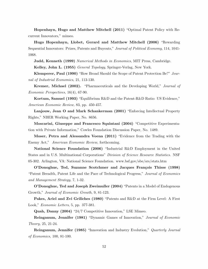
Hopenhayn, Hugo and Matthew Mitchell (2011) “Optimal Patent Policy with Re-

current Innovators,”mimeo.

Hugo Hopenhayn, Llobet, Gerard and Matthew Mitchell (2006) “Rewarding

Sequential Innovators: Prizes, Patents and Buyouts,”Journal of Political Economy, 114, 1041-

1068.

Judd, Kenneth (1999) Numerical Methods in Economics, MIT Press, Cambridge.

Kelley, John L. (1955) General Topology, Springer-Verlag, New York.

Klemperer, Paul (1990) “How Broad Should the Scope of Patent Protection Be?”Jour-

nal of Industrial Economics, 21, 113-130.

Kremer, Michael (2002). “Pharmaceuticals and the Developing World,” Journal of

Economic Perspectives, 16(4), 67-90.

Kortum, Samuel (1993) “Equilibrium R&D and the Patent-R&D Ratio: US Evidence,”

American Economic Review, 83, pp. 450-457.

Lanjouw, Jean O and Mark Schankerman (2001) “Enforcing Intellectual Property

Rights,”NBER Working Paper, No. 8656.

Moscarini, Giuseppe and Francesco Squintani (2004) “Competitive Experimenta-

tion with Private Information,”Cowles Foundation Discussion Paper, No. 1489.

Moser, Petra and Alessandra Voena (2011) “Evidence from the Trading with the

Enemy Act,” American Economic Review, forthcoming.

National Science Foundation (2006) “Industrial R&D Employment in the United

States and in U.S. Multinational Corporations”Division of Science Resource Statistics. NSF

05-302. Arlington, VA: National Science Foundation. www.bsf.gov/sbe/srs/stats.htm

O’Donoghue, Ted, Suzanne Scotchmer and Jacques François Thisse (1998)

“Patent Breadth, Patent Life and the Pace of Technological Progress,”Journal of Economics

and Management Strategy, 7, 1-32.

O’Donoghue, Ted and Joseph Zweimuller (2004) “Patents in a Model of Endogenous

Growth,”Journal of Economic Growth, 9, 81-123.

Pakes, Ariel and Zvi Griliches (1980) “Patents and R&D at the Firm Level: A First

Look,”Economic Letters, 5, pp. 377-381.

Quah, Danny (2004) “24/7 Competitive Innovation,”LSE Mimeo.

Reinganum, Jennifer (1981) “Dynamic Games of Innovation,” Journal of Economic

Theory, 25, 21-24.

Reinganum, Jennifer (1985) “Innovation and Industry Evolution,”Quarterly Journal

of Economics, 100, 81-100.

52

Romer, Paul M. (1990) “Endogenous Technological Change,”Journal of Political Econ-

omy, 98, S71-S102.

Ross, Sheldon (1996) Stochastic Processes, John Wiley & Sons, Inc.

Scotchmer, Suzanne (1999) “On the Optimality of the Patent System,” The Rand

Journal of Economics, 30, 181-196.

Scotchmer, Suzanne (2005) Innovations and Incentives, MIT Press, Cambridge, Massa-

chusetts.

Segal, Ilya and Michael Whinston (2007) “Anti-Trust in Innovative Industries,”

American Economic Review, 97, 1703-1730.

Tandon, Pankaj (1982) “Optimal Patents with Compulsory Licensing,”Journal of Po-

litical Economy 90(3), 470-486.

Taylor, Curtis (1995) “Digging for Golden Carrots: An Analysis of Research Tourna-

ments,”American Economic Review, 85, 872-890.

Tirole, Jean (1988) The Theory of Industrial Organization, MIT Press, Cambridge,

Massachusetts.

Stokey, Nancy (1995) “R&D and Economic Growth”Review of Economic Studies, 62,

pp. 469-489.

Stokey, Nancy and Robert Lucas with E. Prescott (1989) Recursive Methods in

Economic Dynamics, Harvard University Press.

53

Tables

Note: Tables 1-5 give the results of the numerical computations with ρ = 0.05 under three different IPR

policy regimes. Tables 1-4 consider a different environment (quick catch-up, slow catch-up, licensing

and leapfrogging) at a time, whereas Table 5 combines the latter three environments (slow catch-up,

licensing and leapfrogging). Table 6 reports the robustness checks of the state-dependent results of

Table 5 with alternative step sizes and R&D elasticity parameters. Depending on the applicability and

necessity, Tables 1-6 report the steady-state equilibrium values of the difference in the values v1−v−3

and v0−v−3; the (annual) catch-up and frontier R&D rates of a follower that is one step behind,

(xc∗−1, xf∗−1); the (annual) R&D rate of neck-and-neck competitors, x

∗0; the (annual) R&D rate of one-

step leader, x∗1; fraction of industries in neck-and-neck competition, µ∗0; fraction of industries at a

technology gap of n = 1, 2; the value of “labor share,” ω∗; the ratio of the labor force working in

research; log of initial (annual) consumption, lnC(0); the annual growth rate, g∗; and the welfare level

according to equation (42). It also reports the welfare-maximizing uniform and state-dependent IPR

policies. See text for details.

λ = 1.05, γ = 0.35,B = 0.1

Full IPROptimal

Uniform IPROptimal

State-dependent IPR

η1 0 0 0.71η2 0 0 0.08η3 0 0 0η4 0 0 0η5 0 0 0

x∗−1 0.22 0.22 0.12x∗0 0.35 0.35 0.25x∗1 0.29 0.29 0.41µ∗0 0.24 0.24 0.46µ∗1 0.33 0.33 0.19µ∗2 0.20 0.20 0.13ω∗ 0.95 0.95 0.96

Researcher ratio 0.032 0.032 0.028

lnC (0) 33.78 33.78 34.20g∗ 0.0186 0.0186 0.0204

Welfare 683.0 683.0 692.1

Table 1. Optimal Patent Length in Quick Catch-up Regime

54

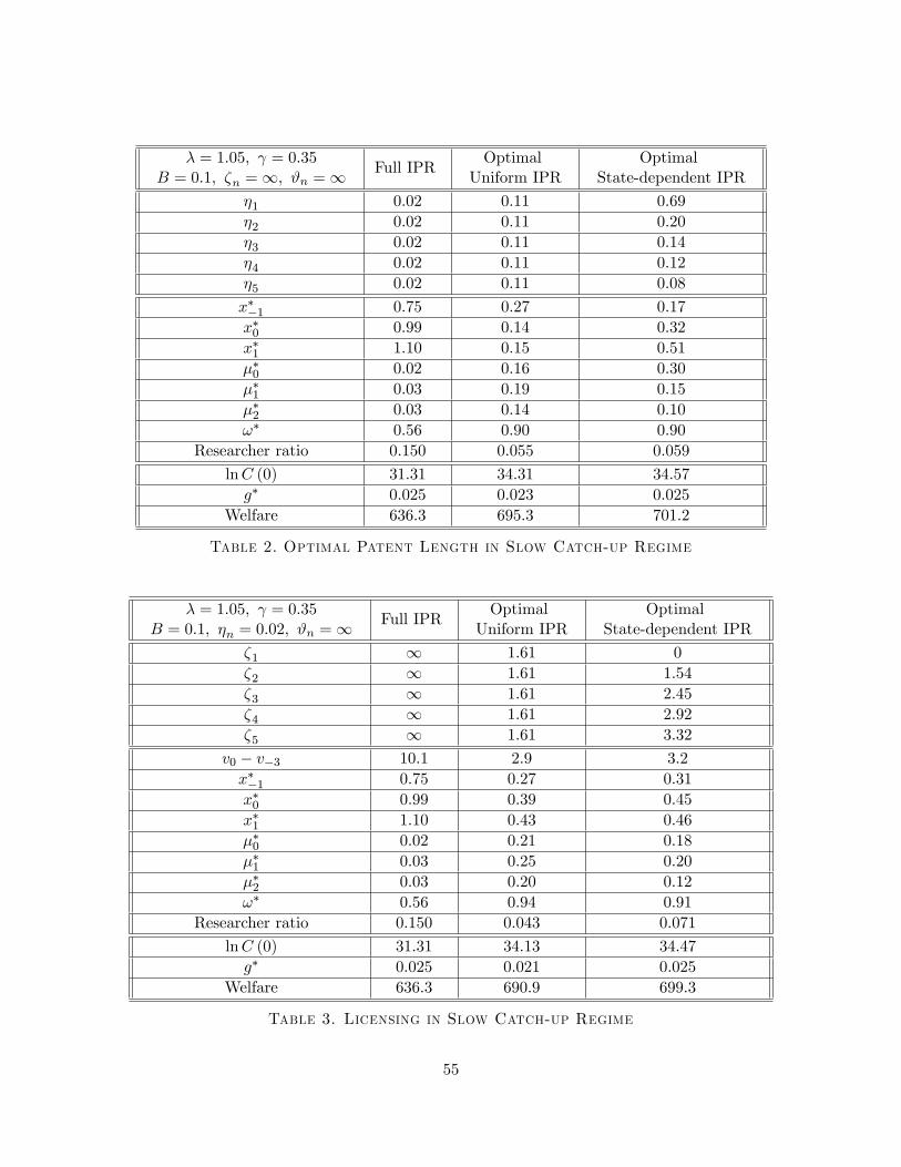
λ = 1.05, γ = 0.35B = 0.1, ζn =∞, ϑn =∞ Full IPR

OptimalUniform IPR

OptimalState-dependent IPR

η1 0.02 0.11 0.69η2 0.02 0.11 0.20η3 0.02 0.11 0.14η4 0.02 0.11 0.12η5 0.02 0.11 0.08

x∗−1 0.75 0.27 0.17x∗0 0.99 0.14 0.32x∗1 1.10 0.15 0.51µ∗0 0.02 0.16 0.30µ∗1 0.03 0.19 0.15µ∗2 0.03 0.14 0.10ω∗ 0.56 0.90 0.90

Researcher ratio 0.150 0.055 0.059

lnC (0) 31.31 34.31 34.57g∗ 0.025 0.023 0.025

Welfare 636.3 695.3 701.2

Table 2. Optimal Patent Length in Slow Catch-up Regime

λ = 1.05, γ = 0.35B = 0.1, ηn = 0.02, ϑn =∞ Full IPR

OptimalUniform IPR

OptimalState-dependent IPR

ζ1 ∞ 1.61 0ζ2 ∞ 1.61 1.54ζ3 ∞ 1.61 2.45ζ4 ∞ 1.61 2.92ζ5 ∞ 1.61 3.32

v0 − v−3 10.1 2.9 3.2x∗−1 0.75 0.27 0.31x∗0 0.99 0.39 0.45x∗1 1.10 0.43 0.46µ∗0 0.02 0.21 0.18µ∗1 0.03 0.25 0.20µ∗2 0.03 0.20 0.12ω∗ 0.56 0.94 0.91

Researcher ratio 0.150 0.043 0.071

lnC (0) 31.31 34.13 34.47g∗ 0.025 0.021 0.025

Welfare 636.3 690.9 699.3

Table 3. Licensing in Slow Catch-up Regime

55

λ = 1.05, γ = 0.35B = 0.1, ηn = 0.02, ζn =∞ Full IPR

OptimalUniform IPR

OptimalState-dependent IPR

ϑ1 ∞ 14 0ϑ2 ∞ 14 18.1ϑ3 ∞ 14 31.3ϑ4 ∞ 14 36.6ϑ5 ∞ 14 43.7

v1 − v−3 21.4 2.7 4.1xc∗−1 0.75 0.15 0.14xf∗−1 0 0.23 0.33x∗0 0.99 0.30 0.29x∗1 1.10 0.30 0.39µ∗0 0.02 0.14 0.12µ∗1 0.03 0.42 0.35µ∗2 0.03 0.22 0.17ω∗ 0.56 0.95 0.94

Researcher ratio 0.150 0.028 0.058

lnC (0) 31.31 35.48 36.17g∗ 0.025 0.026 0.031

Welfare 636.3 720.0 735.9

Table 4. Leapfrogging in Slow Catch-up Regime

56

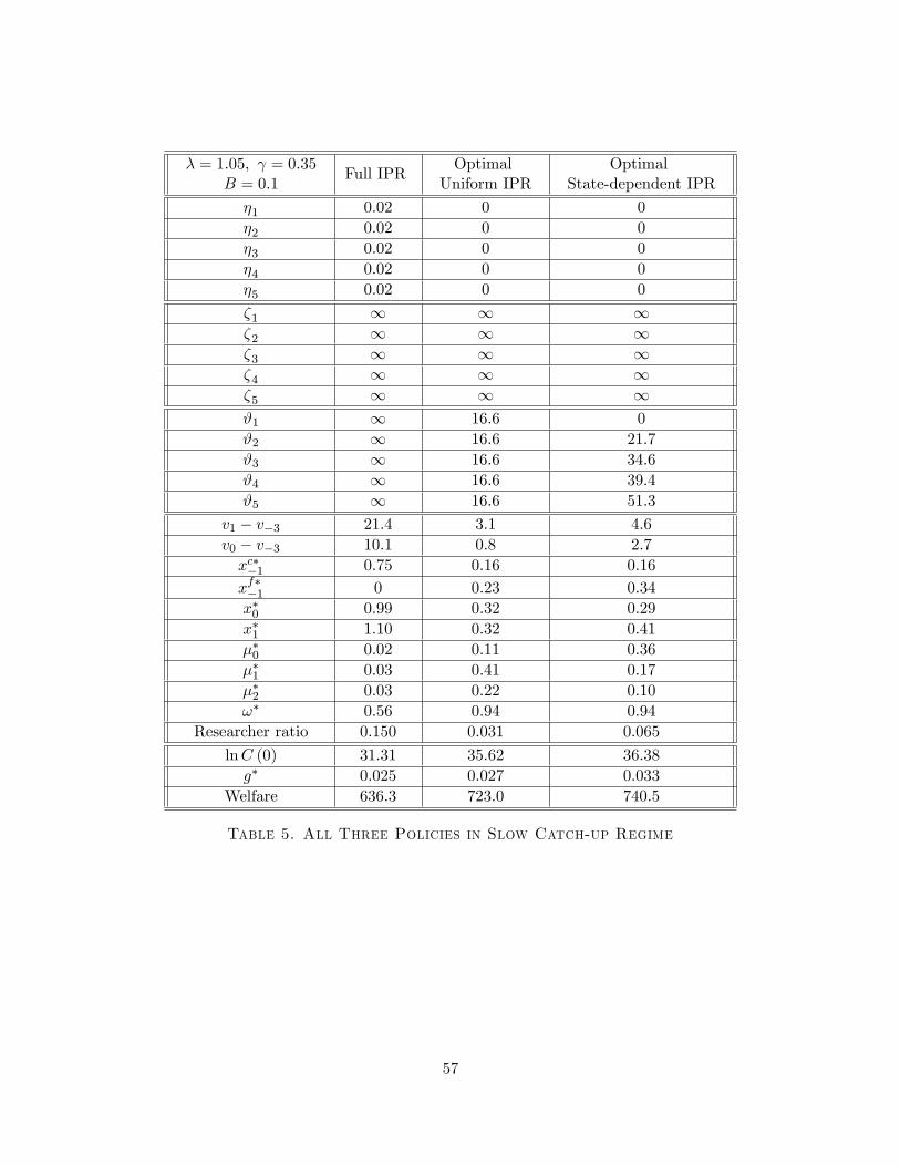
λ = 1.05, γ = 0.35B = 0.1

Full IPROptimal

Uniform IPROptimal

State-dependent IPR

η1 0.02 0 0η2 0.02 0 0η3 0.02 0 0η4 0.02 0 0η5 0.02 0 0

ζ1 ∞ ∞ ∞ζ2 ∞ ∞ ∞ζ3 ∞ ∞ ∞ζ4 ∞ ∞ ∞ζ5 ∞ ∞ ∞ϑ1 ∞ 16.6 0ϑ2 ∞ 16.6 21.7ϑ3 ∞ 16.6 34.6ϑ4 ∞ 16.6 39.4ϑ5 ∞ 16.6 51.3

v1 − v−3 21.4 3.1 4.6v0 − v−3 10.1 0.8 2.7xc∗−1 0.75 0.16 0.16xf∗−1 0 0.23 0.34x∗0 0.99 0.32 0.29x∗1 1.10 0.32 0.41µ∗0 0.02 0.11 0.36µ∗1 0.03 0.41 0.17µ∗2 0.03 0.22 0.10ω∗ 0.56 0.94 0.94

Researcher ratio 0.150 0.031 0.065

lnC (0) 31.31 35.62 36.38g∗ 0.025 0.027 0.033

Welfare 636.3 723.0 740.5

Table 5. All Three Policies in Slow Catch-up Regime

57

κ = 0.1

OptimalState-

dependentIPR

γ = 0.1B = 0.04

OptimalState-

dependentIPR

γ = 0.6B = 0.2

OptimalState-

dependentIPR

λ = 1.01B = 0.35

OptimalState-

dependentIPR

λ = 1.20B = 0.024

η1 0 0 0 0η2 0 0 0 0η3 0 0 0 0η4 0 0 0 0η5 0 0 0 0

ζ1 ∞ ∞ ∞ ∞ζ2 ∞ ∞ ∞ ∞ζ3 ∞ ∞ ∞ ∞ζ4 ∞ ∞ ∞ ∞ζ5 ∞ ∞ ∞ ∞ϑ1 0 0 3.6 0ϑ2 16.7 12.6 5.5 33.4ϑ3 35.6 20.0 8.9 82.3ϑ4 44.8 23.0 12.3 100.7ϑ5 54.0 32.9 15.8 128.7

v1 − v−3 4.1 4.0 1.3 17.5v0 − v−3 2.6 1.6 0.8 5.2xc∗−1 0.23 0.06 0.69 0.02xf∗−1 0.28 0.61 0.88 0.10x∗0 0.27 0.42 0.97 0.10x∗1 0.29 0.98 1.24 0.10µ∗0 0.20 0.01 0.10 0.06µ∗1 0.47 0.15 0.26 0.48µ∗2 0.19 0.09 0.11 0.22ω∗ 0.95 0.90 0.97 0.11

Researcher ratio 0.011 0.161 0.048 0.087

lnC (0) 36.08 37.54 13.80 118.35g∗ 0.027 0.044 0.026 0.035

Welfare 732.4 768.3 286.3 2381.2

Table 6. All Three Policies in Slow Catch-up Regime - Robustness Checks

58

Figures

050

100

150

1980 1985 1990 1995 2000 2005Fiscal Year

Sector: NAICS­511210 (Software Production)

Relative to the Sector AverageR&D by Microsoft

Figure 1

05

1015

2025

1980 1985 1990 1995 2000 2005Fiscal Year

Sector: NAICS­511210 (Software Production)

Relative to the Sector AverageR&D by Top­10 (Except Microsoft)

Figure 2

59

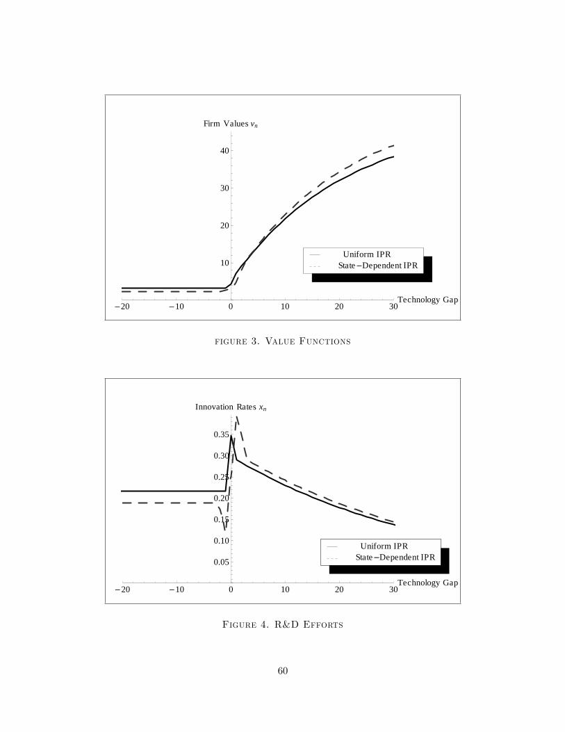
20 10 0 10 20 30Technology Gap

10

20

30

40

Firm Values vn

State Dependent IPRUniform IPR

figure 3. Value Functions

20 10 0 10 20 30Technology Gap

0.05

0.10

0.15

0.20

0.25

0.30

0.35

Innovation Rates xn

State Dependent IPRUniform IPR

Figure 4. R&D Efforts

60

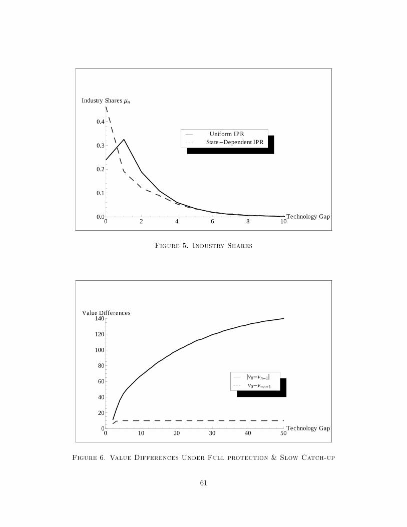
0 2 4 6 8 10Technology Gap0.0

0.1

0.2

0.3

0.4

Industry Shares n

State Dependent IPRUniform IPR

Figure 5. Industry Shares

0 10 20 30 40 50Technology Gap0

20

40

60

80

100

120

140Value Differences

v0 v n 1

v0 vn 1

Figure 6. Value Differences Under Full protection & Slow Catch-up

61