High Throughput Sequence (HTS) data analysis 1.Storage and retrieving of HTS data. 2.Representation...
26
High Throughput Sequence (HTS) data analysis 1.Storage and retrieving of HTS data. 2.Representation of HTS data. 3.Visualization of HTS data. 4.Discovering genomic patterns from HTS data.
-
Upload
mariah-angela-atkinson -
Category
Documents
-
view
254 -
download
5
Transcript of High Throughput Sequence (HTS) data analysis 1.Storage and retrieving of HTS data. 2.Representation...

High Throughput Sequence (HTS) data analysis
1. Storage and retrieving of HTS data.
2. Representation of HTS data.
3. Visualization of HTS data.
4. Discovering genomic patterns from HTS data.
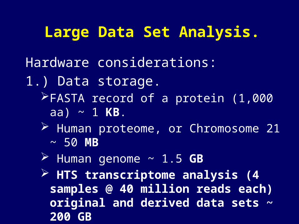
Large Data Set Analysis.
Hardware considerations:
1.) Data storage. FASTA record of a protein (1,000 aa) ~ 1 KB. Human proteome, or Chromosome 21 ~ 50 MB Human genome ~ 1.5 GB HTS transcriptome analysis (4 samples @ 40
million reads each) original and derived data sets ~ 200 GB

Large Data Set Analysis.
Hardware considerations:
2.) Processors and RAM. Comparison: tbalstn of 5 protein sequences
against 1.2GB genome, ~15 sec CPU time. Map a single 10 M reads illumina run to human genome ~15,000 CPU sec (> 4 hours).
When RAM < data size, the computer will come to a crawl.
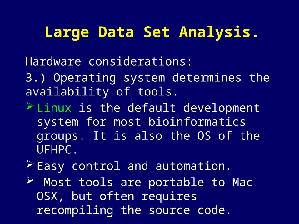
Large Data Set Analysis.
Hardware considerations:
3.) Operating system determines the availability of tools. Linux is the default development system for most
bioinformatics groups. It is also the OS of the UFHPC.
Easy control and automation. Most tools are portable to Mac OSX, but often
requires recompiling the source code.

Observe: demanding computation for large data set analysis.

High Throughput DNA-Sequencing (HTS)
data analysis
1. Sources and representation of HTS data.
2. Visualization of HTS data.
3. Discovering genomic pattern from HTS data.
4. Integrated data analysis and hypothesis-generating exploration.
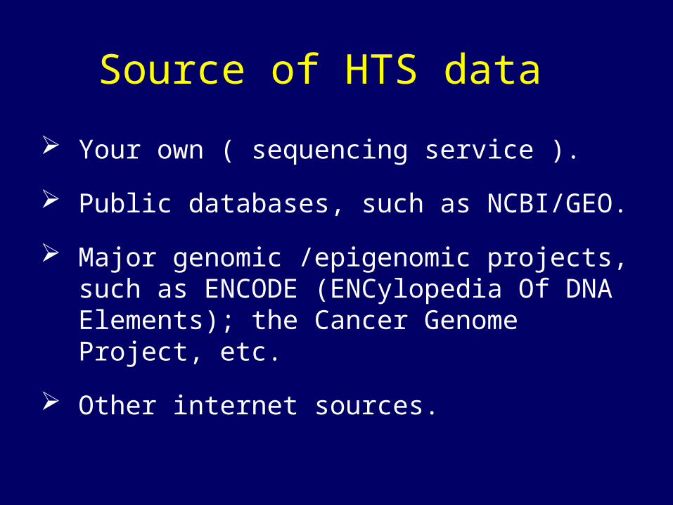
Your own ( sequencing service ).
Public databases, such as NCBI/GEO.
Major genomic /epigenomic projects, such as ENCODE (ENCylopedia Of DNA Elements); the Cancer Genome Project, etc.
Other internet sources.
Source of HTS data
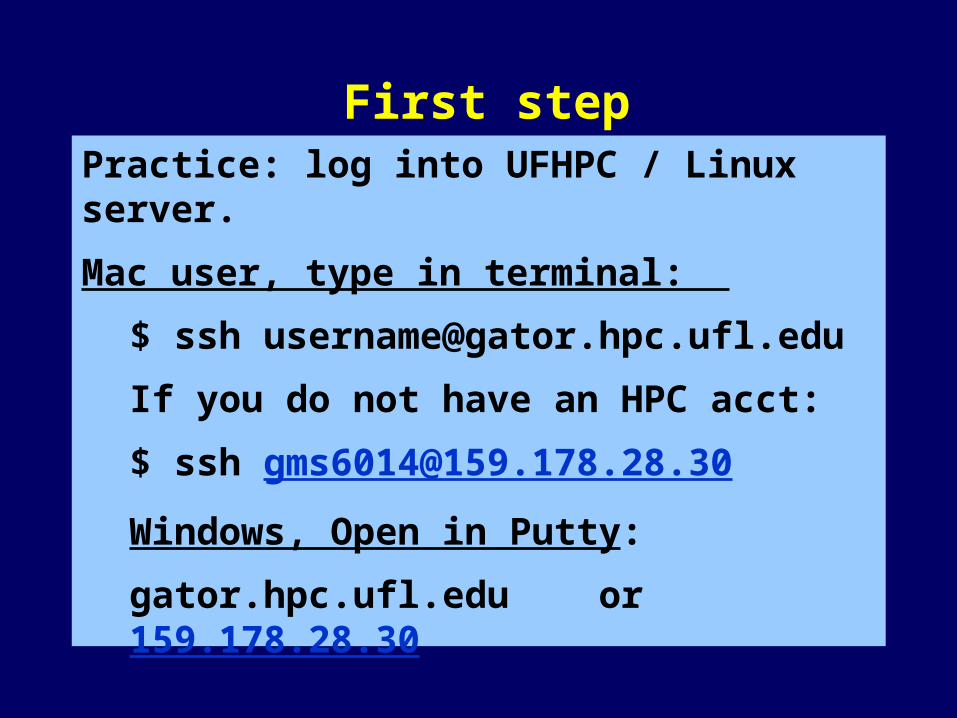
Practice: log into UFHPC / Linux server.
Mac user, type in terminal:
$ ssh [email protected]
If you do not have an HPC acct:
$ ssh [email protected]
Windows, Open in Putty:
gator.hpc.ufl.edu or 159.178.28.30
First step
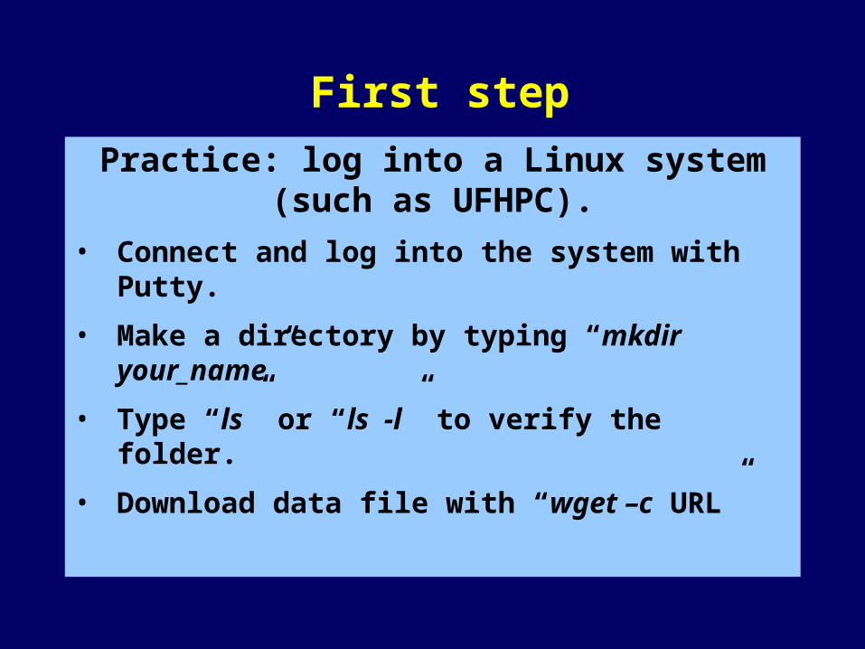
Practice: log into a Linux system (such as UFHPC).
• Connect and log into the system with Putty.
• Make a directory by typing “mkdir your_name”
• Type “ls” or “ls -l” to verify the folder.
• Download data file with “wget –c URL”
First step
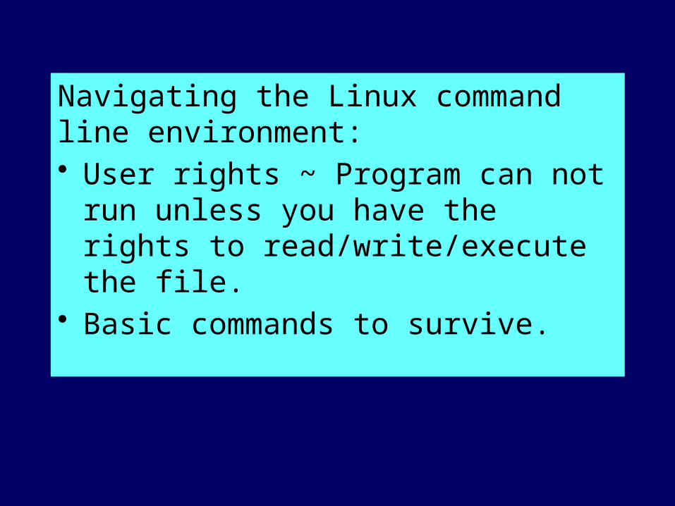
Navigating the Linux command line environment:• User rights ~ Program can not run unless
you have the rights to read/write/execute the file.
• Basic commands to survive.
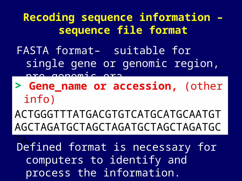
Recoding sequence information – sequence file format
FASTA format– suitable for single gene or genomic region, pre-genomic era.
> Gene_name or accession, (other info)
ACTGGGTTTATGACGTGTCATGCATGCAATGTAGCTAGATGCTAGCTAGATGCTAGCTAGATGCTA….
Defined format is necessary for computers to identify and process the information.

Recording sequence reads from the machine – FASTQ
FASTA:>My_sequenceAATTACGCGCGATACGAT
FASTQ:@My_sequenceAATTACGCGCGATACGAT+My_sequence qualityefcfffffcfeeYBBsdf
Recording of quality assessment allows filtering based on sequence quality.

Paint the sequence reads to the genome
HTS reads@reads_1AATTACGCGCGATACGAT+efcfffffcfeeYBBsdf@reads_2ACCGAGGCGCGTATGTCT+efcfffffcfeeYBBsea….@reads_1,000,001
Corresponding location on the
genomeELAND (Illumina)
Bowtie, etc.
ChIP-Seq; RNA-Seq
De novo assembly of genomes,chromatin conformation, genomic abnormality, etc…

Recording sequence and quality information
FASTQ format = FASTA + Quality
@HWI-EAS209_0006_FC706VJ:5:58:5894:21141#ATCACG/1TTAATTGGTAAATAAATCTCCTAATAGCTTAGATNTTACCTTNNNNNNNNNNTAGTTTCTT+HWI-EAS209_0006_FC706VJ:5:58:5894:21141#ATCACG/1!"#$%&'()*+,-./0123456789:;<=>?@ABCDEFGHIJKLMNOPQabdefghadfda
• Two identification lines (@, +) for each sequence.• Identification line format depends on specific
sequencing platform.• Quality line using characters representing integer
values.
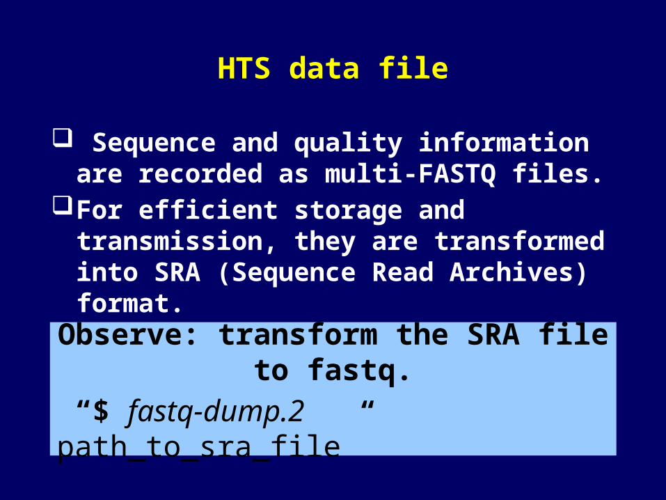
HTS data file
Sequence and quality information are recorded as multi-FASTQ files.
For efficient storage and transmission, they are transformed into SRA (Sequence Read Archives) format.
Observe: transform the SRA file to fastq.
“$ fastq-dump.2 path_to_sra_file”

Representation of (HTS) data – BED (Browser Extensible Data) file
chr2 10000192 10000217 U0 0 + chr2 10000227 10000252 U1 0 -chr2 10000310 10000335 U2 0 +chr3 10000496 10000521 U1 0 -chr2 10000556 10000581 U2 0 +
Chrom. Start End name Scor Strand
With the completion of the genome, there is no need to record the base pair identity (if it is the same as the reference genome).
Detailed description of genomic data formats: http://genome.ucsc.edu/FAQ/FAQformat.html
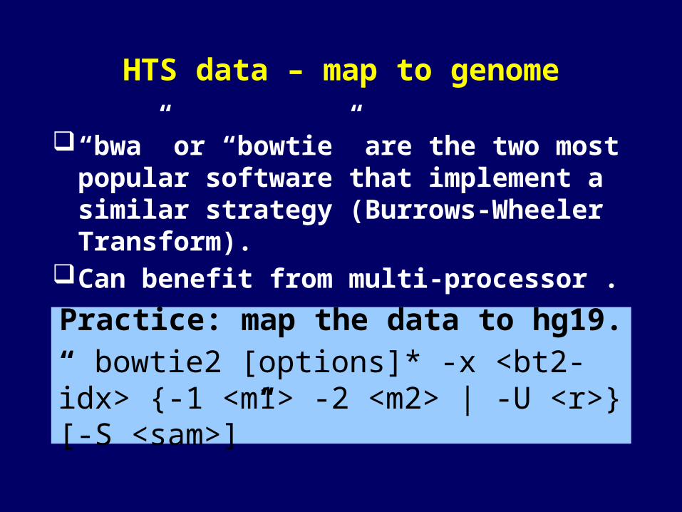
HTS data – map to genome
“bwa” or “bowtie” are the two most popular software that implement a similar strategy (Burrows-Wheeler Transform).
Can benefit from multi-processor .
Practice: map the data to hg19.
“ bowtie2 [options]* -x <bt2-idx> {-1 <m1> -2 <m2> | -U <r>} [-S <sam>]”
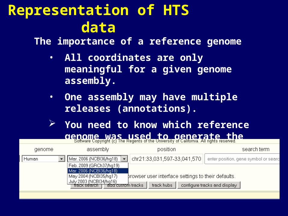
Representation of HTS data
The importance of a reference genome
• All coordinates are only meaningful for a given genome assembly.
• One assembly may have multiple releases (annotations).
You need to know which reference genome was used to generate the BED file.

Retrieving HTS data Retrieving HTS data from the web using
wget.
Loading to and unloading data from UFHPC (check with HPC instructions).
How to gain knowledge from HTS data
Visualization of HTS data.
Discovering genomic patterns.
Identifying novel mechanism – hypothesis generation.

Visualization of HTS data.
Simple visualization - distribution of tags (or normalized values).
Barski et al. (2007) Cell
chr4 0 200 0chr4 200 400 2chr4 400 600 13chr4 600 800 35chr4 800 1000 27
Chr. ChrStart ChrEnd Value
BedGraph file (Wig)

Visualization of HTS data.
Shifting sequence tag position may be necessary to reflect nucleosome positions. In this example the mapping positions were shifted +73bp for forward strain and -73bp for reverse strain to reflect the midpoint of the nucleosome.
Jiang & Pugh, Nat. Rev. Genet., 2009

Visualization of HTS data.
Advanced visualization – depending on purpose of comparison.
Berger et al. (2011) Nature
Example - Circos plot depicts genomic location, chromosomal copy number (red, copy gain; blue, copy loss). Inter-chromosomal translocations (purple) and intra-chromosomal (green) rearrangements observed in primary prostate cancers

Manipulating Deep Seq data with Galaxy
Practice & Observe:
1. Load the PolII.H99.Bed file to Galaxy with the Get Data tool. Select “D. melanogaster Apr. 006 (BDGP R5/dm3) (dm3)” as the database
2. Sort data based on chromosome location c2.
3. Filter out lines with U0 with the expression c4!=‘U2’
4. Extract genomic sequences.

Visualizing Deep Seq data with UCSC genome browser
Practice & Observe I:
1. Load the PolII.H99.Bed file as custom track to the browser by copy/past the URL link.
2. View ‘dense’ and then ‘full’ presentation of the track.

Visualizing Deep Seq data with UCSC genome browser
Practice & Observe II:
1. Save the landmark.bed file to your local computer. View the contents with Notepad.
2. Load the local file to the UCSC browser.
3. Edit the color value, save, resubmit, and observe the differences.