Integrated Master in Chemical Engineering

Integrated Master in Chemical Engineering

Oxygen diffusion through polystyrene flasks -

model development and verification

Master Thesis

of

Guilherme André Ferreira Leite

Developed for Dissertation Class

in

University of Maryland, Baltimore County

Chemical Engineering Department

July 2010

UMBC Advisors:

Dr. Govind Rao

Dr. Yordan Kostov

Acknowledgments

In the first place I would like to thank my supervisor, Dr. Yordan Kostov, for helping

me with his bright advices and guiding.

A special thanks to Dr. Govind Rao for letting me work in his lab and for offer me a

very helpful English course.

To all lab group, a big thank for all the support provided.

I also like to thank Reitoria da Universidade do Porto for financing offer.

The biggest thank goes to my mother, Júlia Leite and my father, António Leite for

contribute, support and gave me all the important things in life. Definitely, everything that I

accomplish or will accomplish I own them.

Finally, to my friend Joana Loureiro for the help and support gave in this last 5 years

and most of all in this 5 months adventure in the United States of America. Also thank you to

João Silva for share this 5 months journey with me.

Abstract

Oxygen concentration in polystyrene flasks during cell culture is typically monitored

with a patch, in situ. This unfamiliar surface disturbs the cells growth and may cause

biofouling. In order to avoid this condition the location of the oxygen sensor on the external

surface of the flask was considered. Nevertheless the flask wall is reasonably thick, therefore

was imperative to decrease the wall thickness without compromising the sterility of the flask

and analyze the oxygen diffusion through the polystyrene.

The evaluation set up necessary to investigate the oxygen diffusion includes 1 mm and

1.7 mm thick sensor; optical adhesive, silicone and glass, black epoxy, two standard epoxy

mix with graphite, casting resin and bismuth alloy as for encapsulation material. In addition

different drillings were made in order to decrease the wall thickness. Furthermore the oxygen

diffusion coefficient in polystyrene was calculated.

This study proved that it is possible leaving only a 100 micron membrane and still

maintained the sterility of the flask. In order to oxygen to be sensitive the back and side of

the membrane have to be impermeable to oxygen. The oxygen diffusion coefficient

calculated is 4x10-8cm2 s-1.

Keywords: Oxygen diffusion, polystyrene flask, cell culture, monitoring, fluorescence

i

Index

Index .......................................................................................................... i

Figure Index ............................................................................................... iii

Notation and Glossary ..................................................................................... v

1 Introduction ........................................................................................... 1

1.1 Project Presentation .......................................................................... 1

1.2 Work contribution ............................................................................. 2

1.3 Theory ........................................................................................... 2

1.3.1 Fluorescence ............................................................................................. 3

1.3.2 Fluorophore .............................................................................................. 5

1.3.3 Fluorescence Measurements ......................................................................... 6

1.3.4 Cell Culture .............................................................................................. 10

1.3.5 Oxygen diffusion ....................................................................................... 11

2 State of Art .......................................................................................... 13

3 Technical Description and Results Discussion ................................................ 16

4 Conclusions ......................................................................................... 38

5 Work Evaluation .................................................................................... 39

5.1 Accomplish Goals ............................................................................. 39

5.2 Limitations and Future Improvements ................................................... 39

5.3 Final Appreciation ........................................................................... 40

6 References .......................................................................................... 41

Annex 1 Experimental Procedure for Oxygen Sensor Fabrication ......................... 44

Annex 2 G-codes ..................................................................................... 45

2.1 1.4 mm depth ................................................................................. 45

2.2 1.4 mm depth with 3 seconds dwell ...................................................... 49

2.3 1.76 mm depth with 10 micron side and inverted “s” path ......................... 53

2.4 1.76 mm depth with 10 micron side and side to the center path .................. 54

2.5 1.79 mm depth with 10 micron side and center to side path ....................... 55

ii

2.6 1.83 mm depth ................................................................................ 57

iii

Figure Index

Figure 1- Description of the Jablonski diagram ....................................................... 3

Figure 2 – RUDPP structure ............................................................................... 6

Figure 3 – Frequency modulation measurement scheme ............................................. 8

Figure 4 – Optical Coaster ............................................................................... 10

Figure 5 - Growth cells curve ........................................................................... 11

Figure 6 - Polystyrene Flask ............................................................................. 16

Figure 7 - Manual drilling machine with drill bit .................................................... 17

Figure 8 - Illustrative example of the polystyrene membrane shape ............................. 17

Figure 9 - Polystyrene membrane profile ............................................................. 18

Figure 10 - Polystyrene membrane with encapsulate sensor ...................................... 18

Figure 11 - Lifetime over the time in polystyrene membrane ..................................... 19

Figure 12 - Flask cross section for optical adhesive experiment .................................. 20

Figure 13 - Lifetime over time in flask ................................................................ 21

Figure 14 - CNC Milling Machine ........................................................................ 22

Figure 15 - Lifetime over time for optical adhesive encapsulation ............................... 22

Figure 16 - Flask cross section for optical adhesive experiment with thin sensor and

membrane .................................................................................................. 23

Figure 17 - Lifetime for optical adhesive encapsulation, thin sensor and membrane ......... 24

Figure 18 - Flask cross section for silicone encapsulation .......................................... 24

Figure 19 - Lifetime for silicone encapsulation ...................................................... 25

Figure 20 - Lifetime comparison between sensor and patch for silicone encapsulation and

cell culture ................................................................................................. 26

Figure 21 - Lifetime for silicone encapsulation and PAN glass isolation in a cell culture ..... 27

Figure 22 - PMMA plate .................................................................................. 28

Figure 23 - Cross section for black epoxy encapsulation ........................................... 28

Figure 24 - Lifetime for black epoxy encapsulation ................................................. 29

iv

Figure 25 - Lifetime for PVA and black epoxy encapsulation ...................................... 29

Figure 26 - Lifetime for epoxy encapsulation ........................................................ 30

Figure 27 - Lifetime for resin encapsulation ......................................................... 31

Figure 28 - Lifetime for bismuth alloy encapsulation ............................................... 32

Figure 29 - Lifetime comparison between sensor and patch for bismuth alloy encapsulation

with cell culture ........................................................................................... 33

Figure 30 - Lifetime comparison between bismuth alloy encapsulation with hardener

pretreatment and bismuth alloy encapsulation ...................................................... 34

Figure 31 - Oxygen diffusion coefficient in polystyrene testing scheme ......................... 35

Figure 32 - View from the top scheme ................................................................ 35

Figure 33 - Lifetime for silicone encapsulation in glass ............................................ 35

Figure 34 - Concentration profile over the thickness in different times ........................ 36

v

Notation and Glossary

S0

S1

S2

T1

T2

��

�

��

��

�� ø

�

�

�

�

�

�

��

�

�

��

� �

Singlet ground

First electronic states

Second electronic states

First triplet state

Second triplet state

Emission intensity in quencher absence

Emission intensity in quencher present

Stern-Volmer constant

Quencher concentration

Emission intensity at time zero

Time

Phase Angle

Peak to peak height for incident light

Average excitation intensity

Peak to peak height for reflect light

Average emission intensity

Modulation factor

Modulation frequency

Frequency

Diffusion coefficient

Length

Concentration

Initial oxygen concentration

Oxygen concentration for � � � Thickness

Sound wave velocity

Greek Leters

�

��

�� ø

��

Lifetime in quencher presence

Lifetime in quencher absence

Time domain lifetime

Phase lifetime

Modulation lifetime

vi

Acronyms List

RUDPP

LED

FLIM

PMDS

UV

PAN

DMF

PMMA

PVA

Ruthenium (II) tris (4,7-diphenyl-1,10-phenanthroline) Chloride

Light Emitting Diode

Fluorescence lifetime imaging microscopy

Poly (dimethyl siloxane)

Ultraviolet light

Polyacrylonitrile

n,n-Dimethylformamide

Poly (methyl methacrylate)

Polyvinyl alcohol

Introduction 1

1 Introduction

1.1 Project Presentation

The mobility of gases in solid polymers is an amazing subject not only from the

theoretical point of view but also for the practical view.

The oxygen is the most important gas for human and all living creatures in general, so

it is natural that the transport behavior of oxygen is very important for gas separation,

packaging materials, protective coatings and polymer oxidative degradation (Tolosa et al.,

2006). In this particularly case an oxygen diffusion study will be important to increase the

knowledge for subsequent cell culture studies in polystyrene flasks.

Oxygen concentration in polystyrene flasks during cell culture is typically not

monitored as there are no available ports for traditional electrochemical sensors. Such ports

are also not easy to manufacture and it is difficult to sterilize the sensor for use in such

vessels. Partial solution to oxygen concentration monitoring is to use an optical sensor which

is monitored through the transparent wall. However, they are partially invasive and require

positioning of the sensor patch inside the flask in aseptic conditions (Tolosa et al., 2002).

Furthermore, the patch itself present to the cells surface entirely different characteristics

from the inner surface of the flask. This can pose a problem for growing of anchoring cells

(Tolosa et al., 2006). The aim of the project was to evaluate the possibility for positioning of

the oxygen sensor in the external surface of the flask. However the wall of the flask is fairly

thick and different manufacture used different grades of polystyrene for flask production.

Hence it was necessary to evaluate the diffusion coefficient of the oxygen and to search for

methods to decrease the flask wall in a limited size spot without compromising the sterility of

the flask.

With this results a mathematical model capable to predict the response time for

oxygen concentration and thickness variation can be developed.

In order to accomplish this, an oxygen diffusion study through polystyrene flasks was

performed. It tested different encapsulation materials used in order to avoid side diffusion.

Furthermore, the diffusion coefficient of the oxygen in polystyrene was calculated. Since the

study includes cell culture, it was important to study the sterility of the drilled flask. Last but

not the least the decrease of the wall thickness by machining it in order to reduce the

response time is another research goal.

The most important part of this project was to build a measurement setup for oxygen

diffusion evaluation. Here 1 mm and 1.7 mm thick sensor; optical adhesive, silicone and glass,

Introduction 2

black epoxy, two standard epoxy mix with graphite, casting resin and bismuth alloy as for

encapsulation material and different approach were tested to accomplish the objective of

this study.

However the method for oxygen measure as well as the oxygen sensor itself remains

constant in all experimental tests. In order to measure, an optical reader shaped as a

coaster, containing light emitting diode (LED) for excitation and photodiodes for detection

was used (Gupta and Rao, 2003).

The oxygen sensor used is a silicone rubber membrane with an oxygen sensitive dye

ruthenium (II) tris (4,7-diphenyl-1,10-phenanthroline) Chloride (RUDPP). This ruthenium

complex, when excited by a beam light, can show variations in oxygen’s levels as a phase

angle in the fluorescence emission (Randers-Eichhorn et al., 1996).

1.2 Work contribution

The innovation in this study is the ability to measure oxygen without disturbing the

cell culture. Positioning the sensor on the external surface with only 100 micron separation

layer of polystyrene allows avoiding direct contact between the sensor and the cells. Cells are

still growing in their native environment; no foreign surface is presented to the cells; there is

no possibility for chemicals to leach out from the sensor. Furthermore the thin membrane

allows monitoring of the oxygen concentration in conditions close to real time.

1.3 Theory

To study the oxygen diffusion the following scheme was adopted; on one side of the

diffusion membrane the oxygen sensor was positioned. Precautions to isolate the sensor from

the environment in such way that the only place where the diffusion can take place is through

the membrane were taken. Then the oxygen concentration is varied in the other side of the

wall and measure the response time to such changes. As the response time of the sensor itself

is three orders of magnitude shorter than the steady state time through the membrane, this

method is accurate enough to determine the diffusion rate. As fluorescence sensor is being

used, below the principles of operation of such sensors are discussed.

Introduction 3

1.3.1 Fluorescence

In the last two decades the fluorescence became an upcoming method to biochemical

measurements. Cellular and molecular imaging has been the reason why fluorescence became

so popular in nowadays. Fluorescence is so high sensitive that can show the location and also

measure one single molecule (Lakowicz, 2006). This is imperative to accurately measure some

parameters, like the oxygen concentration, in cell cultures. Progress in chemicals, electronics

and materials make the fluorescence sensors developed into more economical and practical

equipment (Tolosa et al., 2006).

The word luminescence appears in the end of the 19 century and described the

emission of the light from every substance and occurs from electronically excited states

(Oxford, 2010). The excited atoms emit photons of electromagnetic energy when they go

back to ground state. The different types of luminescence depend on the nature of the

excited state. The ones referred in this study are the fluorescence and the phosphorescence.

For many considered the father of the fluorescence spectroscopy, Professor Alexander

Jablonski made a diagram with a homonymous name, that depicted the processes that occur

between the absorption and emission of light. Jablonski diagrams are often used to illustrate

a variety of processes that can take place in excited states.

Jablonski diagram is shown on Figure 1.

Figure 1- Description of the Jablonski diagram (Chasteen, 1996)

Introduction 4

In this Jablonski diagram, S0, S1, S2 are the singlet ground, first and second singlet

states, respectively. Singlet is the quantum state where two spin angular momenta of

electrons cancel each other, resulting in zero spin (Oxford, 2010). T1 and T2 are the first and

second triplet state, respectively. Triplet is an atomic state where exist a non zero spin

(Oxford, 2010). In each of the electronic states the fluorescent substance or fluorophore can

have different excited vibrational states.

Fluorescence, F, is defined as the light emission from an excited singlet state or

between states of the same spin state. The typical fluorescence lifetime is close to 10

nanoseconds (10 x 10-9 seconds) (Lakowicz, 2006). The lifetime of a fluorophore is the average

time since the excitation until the return to the ground state. Since the internal conversion,

normally condensed molecules that quickly relax to S1, usually take place in 10-12 seconds or

less, the conversion is complete before the emission. Fluorescence is independent of the

temperature (Oxford, 2010).

Phosphorescence, P, is light emission from triplet excited state. This occurs because

molecules in first singlet state can experience an exchange to the first triplet state, in a

process called intersystem crossing. The average phosphorescence lifetime is between

milliseconds and seconds but sometimes the phosphorescence lifetime can reach minutes or

even hours, like some clockwise for example. In this way and at the same temperature, since

the increase of the temperature decrease the afterglow, the phosphorescence lifetime is

greater than fluorescence lifetime. Although not always the distinction between the

fluorescence and the phosphorescence is clear (Lakowicz, 2006).

Analyzing the Jablonski diagram it is also possible to observe that absorption energy is

usually more than the emission energy. Stokes was the first to notice this phenomenon

(Stokes, 1852). In general, fluorescence results in lower emission energy or longer

wavelengths while in phosphorescence occurs the opposite.

Nevertheless the intensity of fluorescence can be decreased by different ways in a

process termed quenching. One mechanism of quenching is when fluorophores form with

quenchers a non fluorescent complex. This process is termed static quenching because it

happens in ground state. Attenuation of the incident light by fluorophores or other absorbing

species is another form of quenching, in this case a non molecular one (Lakowicz, 2006).

However the quenching mechanism that matters the most for this study is the

collisional or dynamic quenching. This type of quenching takes place when other molecule in

solution, called quencher, collides with the excited fluorophore. In this way the fluorophore

is desactived, without any chemical alteration in the molecules.

Introduction 5

The decreasing of the quenching intensity is described by the Stern-Volmer equation

given by Equation (1).

�� 1 � �� (1)

where �� and � are the emission intensities in absence of the quencher and presence

of quencher , respectively, �� is the lifetime in absence of quencher, � the lifetime in

quencher presence, �� is the Stern-Volmer quenching constant and �� is for the quencher

concentration (Demas et al., 1995). Since in this study is admit only dynamic quenching the

equality �� can me made (Tolosa et al., 2006).

The sensitivity of the fluorophore to a quencher is denoted by the Stern Volmer

quenching constant. The more the fluorophore is free in solution and also in the surface of

the molecules the larger going to be the �� constant (Lakowicz, 2006).

An ample diversity of molecules can perform as collisional quenchers like oxygen,

halogens, amines and electron. Though molecular oxygen is an exceptional quencher of both

singlet and triplet excited states of organic molecules. In this way fluorescence,

phosphorescence and even the triplet absorption intensities of an organic molecule, generally

supported by a solid polymer, will change according with a free or not free oxygen

environment. The support of a solid polymer guarantees, for the majority of the sensors, that

the system satisfies the ideal Stern-Volmer equation because practically every luminescent

sensors will respond not only to oxygen but also to proteins, solvents, metal ions, oxidants,

reductants (Demas et al., 1995). In this way the oxygen sensor has to be isolated from the

interferences discussed earlier and at the same time must provide full access to oxygen.

1.3.2 Fluorophore

The fluorophore or fluorescence substance is a very important part of the fluorescence

measurement. The fluorophore properties determine the set up instrumentation necessary for

the measurement as well as the sensitivity for the parameter of interested (Lakowicz, 2006)

(Tolosa et al., 2006).

Fluorophore can be divided in two main categories: intrinsic and extrinsic.

Introduction 6

Intrinsic fluorophores crop up naturally. Some of the intrinsic fluorophores known are

the aromatic amino acids, NADH, chlorophyll to name a few (Lakowicz, 2006). In other hand

extrinsic fluorophore are added to the molecules to either provide fluorescence when none

exists before or just to change some spectral properties of the molecule. Dansyl, fluorescein

and rhodamine are some examples of extrinsic fluorophores (Lakowicz, 2006).

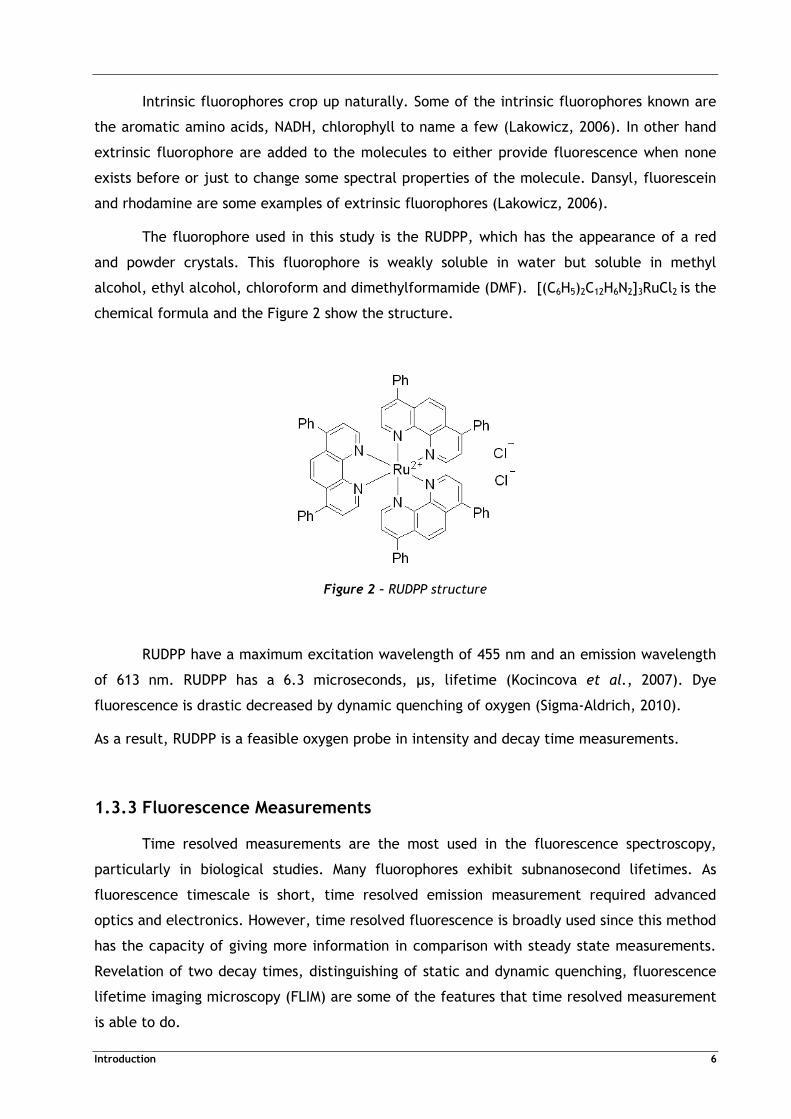
The fluorophore used in this study is the RUDPP, which has the appearance of a red

and powder crystals. This fluorophore is weakly soluble in water but soluble in methyl

alcohol, ethyl alcohol, chloroform and dimethylformamide (DMF). [(C6H5)2C12H6N2]3RuCl2 is the

chemical formula and the Figure 2 show the structure.

Figure 2 – RUDPP structure

RUDPP have a maximum excitation wavelength of 455 nm and an emission wavelength

of 613 nm. RUDPP has a 6.3 microseconds, µs, lifetime (Kocincova et al., 2007). Dye

fluorescence is drastic decreased by dynamic quenching of oxygen (Sigma-Aldrich, 2010).

As a result, RUDPP is a feasible oxygen probe in intensity and decay time measurements.

1.3.3 Fluorescence Measurements

Time resolved measurements are the most used in the fluorescence spectroscopy,

particularly in biological studies. Many fluorophores exhibit subnanosecond lifetimes. As

fluorescence timescale is short, time resolved emission measurement required advanced

optics and electronics. However, time resolved fluorescence is broadly used since this method

has the capacity of giving more information in comparison with steady state measurements.

Revelation of two decay times, distinguishing of static and dynamic quenching, fluorescence

lifetime imaging microscopy (FLIM) are some of the features that time resolved measurement

is able to do.

Introduction 7

Time resolved measurements have two major approaches: time domain or pulse

fluorometry and frequency domain fluorometry or phase modulation fluorometry that will be

discussed with more detail in the next sections.

1.3.3.1 Time Domain

Time domain is a method that uses the pulse of the light for excitation of molecules.

Intensity over time is measured subsequent to pulse excitation. The lifetime or the decay

time, ��, is then calculated through Equation (2).

�!�" � �� #�$ %&�� ' (2)

where �!�" is the intensity over time, � is the time and �� is the intensity when � � 0.

Intensity decays are commonly measured by polarizers oriented at 54.7 degrees, avoiding in

this way the effects of the rotational diffusion or the anisotropy (Lakowicz, 2006).

1.3.3.2 Frequency Domain

Alternatively, the frequency domain method, uses intensity modulated light, like

sinusoidal modulation, to excite the sample. The frequency of the incident light is around 100

MHz (in this particular study 75 MHz), to guarantee that the reciprocal frequency is similar to

the reciprocal decay time. Consequently, the emission from the excited fluorophore exhibits

modulation at the same frequency.

Fluorophore lifetime adds a time delay in the emission comparatively to the excitation

time. This delay is the phase angle (ø), between the excitation and the emission, is

illustrated in Figure 3.

Introduction 8

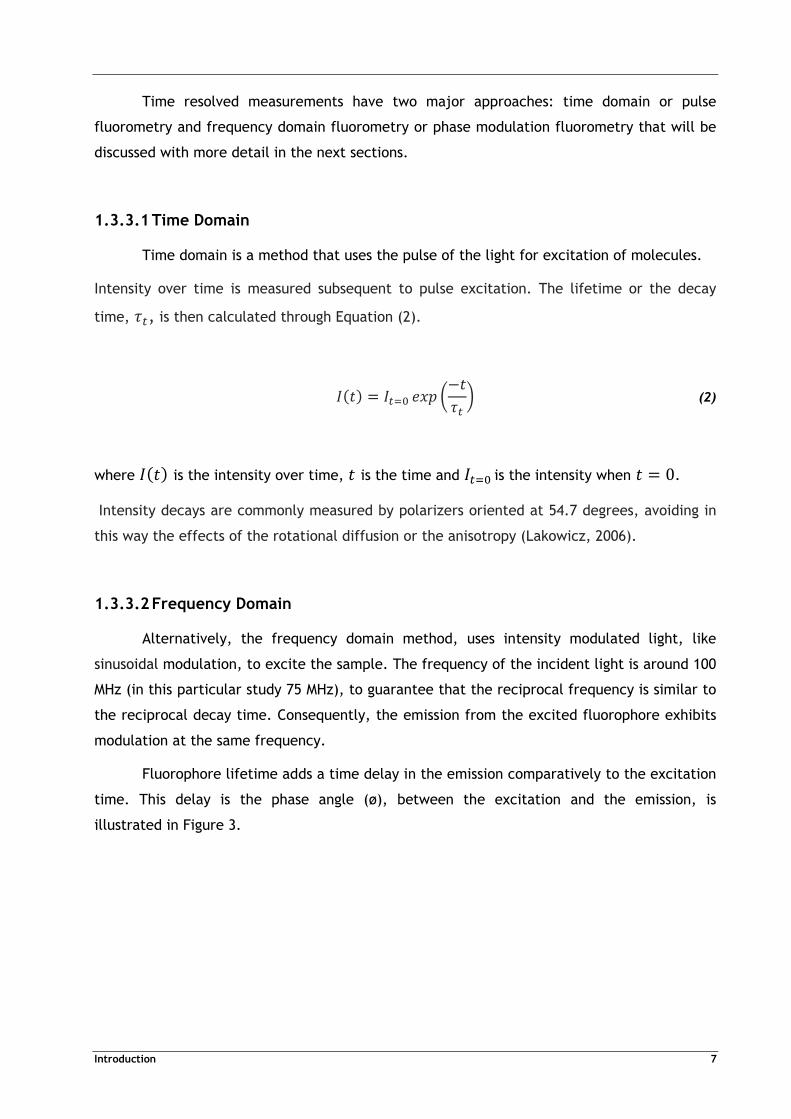
Figure 3 – Frequency modulation measurement scheme (Lakowicz, 2006)

In addition, fluorophore lifetime also reduces the peak to peak emission height

comparatively to the excitation modulation, illustrated as blue line in Figure 3. The reason

for the occurrence of this phenomenon is because several excited fluorophores at the peak of

the excitation maintain the emission even with the excitation at a minimum. The emission

extension depends on the decay time and light modulation frequency (Lakowicz, 2006).

Excitation modulation is the ratio between and �, where is the average excitation

intensity and � is the peak to peak height for incident light, depicted in Figure 3. The

emission modulation, )*, similar to the excitation modulation but relatively to emission is

illustrated as the green line in Figure 3. Emission modulation is measured relatively to the

excitation by a factor � � !�/�"/! /�". In fact � is a demodulation factor but is actually

called modulation (Lakowicz, 2006).

Both phase angle (ø) and modulation (�) can be used to calculated the lifetime

through Equation (3) and Equation (4), respectively. Equation (3) gives the phase lifetime (�ø)

and Equation (4) the modulation lifetime (��).

�ø � �,� ��-!ø" (3)

�� ,� .�,/ & 1 (4)

� � 2 1 � (5)

Introduction 9

The variable ω represents the modulation frequency and � the frequency itself. In

Equation (3) the angle use must be in radians. Equations (3) and (4) are corrected for single

exponential intensity decay. However if the intensity decay is multi or non exponential these

equations calculate only apparent lifetimes, which represents a complex weighted average of

the decay components.

1.3.3.3 Instrumentation

Successful experiments depend on the instrumentation and on some experimental

details that cannot be neglected. Despite of the fact that the light emission can be detected

with high sensitive by powerful sensors which originates signals in substances that practically

do not have fluorescent, it is also true that many different interferences exist like fluorescent

that comes from the solvents, emission from optical components or the polarization and

anisotropy of the emitted light (Lakowicz, 2006).

Formerly, electrodes and fiber optics were used to measure several important

parameters in cell culture or in fermentation. Nevertheless this equipment introduces an

error in the real parameter value. For instance the Clark-type electrode changes not only the

flow conditions in the culture media but also consumes oxygen (Tolosa et al., 2002). Hence

the oxygen concentration measurement is different from the oxygen concentration without

the probe.

Nowadays a fluorometer or optical coaster is a much more reliable and inexpensive

equipment to measure, for example oxygen concentration and pH and above all allows to

measure parameters through a non invasive approach.

One typical fluorometer contains light sources, a photodetector, filters and optics.

Optics will depend of the optical properties of the sensor as well as of the process itself. If it

is necessary to increase the quantity of light that reaches the photodetector, transmission

and collection optics are used. If the sensor is polarized, polarizers have to be used. Filters

are a very important optical part, since they guarantee the separation between excitation

and emission. The light path is also important because the excitation light can take several

directions included into the photodetector. To circumvent this situation the photodetector

should be placed at deep base of one fluorometer with black walls like the one illustrated in

Figure 4.

Introduction 10

Photodetector

Figure 4 – Optical Coaster

Frequently, photodetectors are silicone photodiodes. If greater sensitivity is needed

avalanche photodiodes and photomultipliers should be used (Tolosa et al., 2006).

There are numerous light sources, although LEDs are more desirable because of their low cost

and wide range of frequencies (Tolosa et al., 2006) (Lakowicz, 2006).

For the experiments performed in this study, a fluorometer, like the one shown in Figure 4

was used. The light source used was a LED, placed at 45 degrees to illuminate the sensor and

collect the emitted luminescence light without any mirrors or collecting lenses.

Ultimately, proper spatial orientation of all these components as well as matching the

optical properties of the sample is required for a good and accurate measurement.

1.3.4 Cell Culture

In this study hybridoma cells were used. Hybridomas were produced by hybridization

of a B lymphocyte cell, which have the ability to make the antibody, with myeloma cells,

cancer cells that are capable to multiply indefinitely (Oxford, 2010) (Britannica, 2010). The

fusion of these two cells guarantees a monoclonal antibody production (Britannica, 2010).

LED

Introduction 11

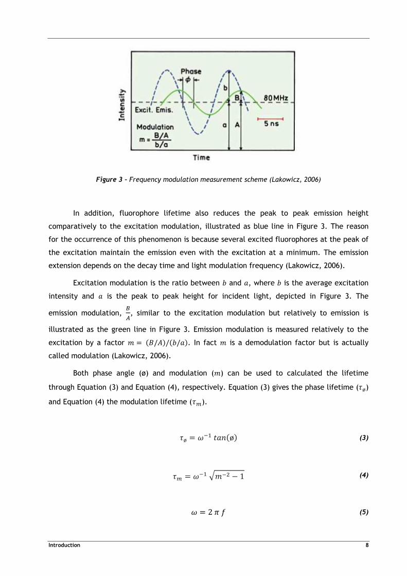
The standard growth curve is depicted in Figure 5.

Figure 5 - Growth cells curve (Decker, 2005)

The lag phase represents the enzymes produced in order to cells growth. In log phase

the cells have an exponential grow, consuming much more oxygen in this phase that all the

others. In stationary phase the growth and death rate are in equilibrium. In death phase the

waste products and absence of nutrients start killing the cells decreasing the oxygen

consumption.

Lifetime theoretical curve of RUDPP, must have a similar look since the lifetime is

inversely proportional to oxygen concentration. When cells consume oxygen there is no free

oxygen to quench the RUDPP fluorescence and therefore the lifetime increase. However when

the cells start to die the free oxygen quenches the fluorescence of RUDPP and consequently

decreases the lifetime.

1.3.5 Oxygen diffusion

In 1855 a major equation was derivated by the physiologist Adolf Fick (Fick's law,

2008). This equation is known by the first Fick’s law and describes the diffusion between two

solutions with different concentrations with the molecules taking the direction from the high

concentration to lower concentration (Fick's law, 2008). However Adolf Fick derivated

another equation termed second Fick’s law. This second equation describes the transient

diffusion for slab geometry.

Time (h)

Introduction 12

Equation (6) describes the second Fick’s Law.

2�2� � �� 2/�2/� (6)

where � is the concentration, � is the time, �� the diffusion coefficient and � is the length

of the wall where diffusion occurs.

Second Fick’s law can be solved analytically for one dimensional slab and the response

time can be found for different thicknesses and different diffusion coefficients. As the

thickness of the membrane is known (measurable with a caliper) the theoretical curve can be

fitted to reflect the experimentally found response time and evaluate in this way the

diffusion coefficient.

Mills and Chang developed a model based on Fick’s law that is capable to predict

oxygen diffusion coefficient (Mills and Chang 1992). In their model one side of the system

(� � 0) is consider to be impermeable to the oxygen. In the other side, when � � �, oxygen

concentration is tested.

The model considers a step change on concentration. Equation (7) and Equation (8)

refers to a concentration changing; zero to 0.21 (oxygen concentration in the air) and 0.21 to

zero respectively.

where �� is the initial oxygen concentration, �� is the oxygen concentration for � � �, � is the time, � the thickness of the polystyrene membrane, � is the length and � !�, �" is the

concentration in order of length and time. Since this study is for oxygen diffusion only the

Equation (7) will be considered.

� !�, �" & �� & �� %1 & 41' 5 !&1"62- � 1 #�$ 7&�� 81 !2- � 1"2 � 9/ �:

;

6�<=> 81!2- � 1" �2 � 9 (7)

� !�, �" & �� & �� 41 5 !&1"62- � 1 #�$ 7&�� 81 !2- � 1"2 � 9/ �:

;

6�<=> 81!2- � 1" �2 � 9 (8)

State of Art 13

2 State of Art

In the early days, the standard approach to determine the diffusion coefficients of

gases by measuring the rate of oxygen permeation across one thin polymer membrane, with a

known area, over the time (Wen, 1993).

Nowadays oxygen quenching has been a well know method to quantify the oxygen

diffusion through polymer films.

In the beginning of sixties Czarnecki and Kryszewski were the first to try measuring the

luminescence quenching in polymers, in particularly a polymethyl methacrylate rod, doped

with naphthalene and other hydrocarbons. In this experiment it was observed that after a

period of time the rod had a phosphorescent zone in the center while in the surroundings a

dark area was visible when brighten by an ultraviolet light. Over time the core became

smaller. The removal of oxygen by setting the rod in a vacuum restores the phosphorescent

zone, proving that the oxygen is a quencher of phosphorescent (Czarnecki and Kryszewski,

1963).

Similar studies were made by Hormats and Unterleitner and by Shaw as well, a few

years later. However, instead of naphthalene to dope the polymethyl methacrylate rod,

triphenylene was used in both cases (Hormats and Unterleitner, 1965) (Shaw, 1967). Shaw

also used phenanthrene (Shaw, 1967). These studies were successful although they have room

temperature phosphorescence as a detection limitation.

In mid seventies Nowakowska et al. studied the oxygen fluorescence quenching in

polystyrene at room temperature (Nowakowska et al., 1976).

A few years later MacCallum and Rudbkin developed a technique to determine the

oxygen diffusion coefficient, for a broad range of temperatures, in polymeric glasses. This

technique consisted in monitoring the quenching of polystyrene excimers (an unstable excited

molecule) (Stevenson, 2005) and (MacCallum and Rudkin, 1978).

Petrak and Holland et al., described a new method for measurement of oxygen

permeability. This technique consisted in examines one sensing film placed between an

oxygen impermeable support and the polymer layer under test. This sensing film possesses

one sensitizer which under excitation produces singlet oxygen that reacts with an oxygen

acceptor, which is directly connected with the absorbance. Changes in the oxygen acceptor

absorbance were used to monitor the oxygen flux that passes through the polymer membrane.

As a result of the absorbance measurement over the time, diffusion coefficients were

determined (Holland et al., 1980) and (Petrak, 1979).

State of Art 14

Despite of this promising technique the complex sample preparations and the slow

experiments make this method difficult to implement.

Cox and Dunn also use the quenching of fluorescence to study the diffusion of oxygen.

However a poly(dimethyl siloxane) (PDMS), unfilled and filled with small fractions of fumed

silica sheet was used. This method consisted in observing the quenching of oxygen in an

organic fluorophore, homogeneously spread into the film, over the time. Along the

experiments, the emission intensity was measure and assumed to correspond to the average

oxygen concentration in the film. Then the emission intensity was converted to concentration

using Stern-Volmer equation (Cox and Dunn, 1986) (Cox and Dunn, 1986) and this assumption

introduced an error in some experimental conditions, since in dynamic conditions the oxygen

concentration calculated from the steady state Stern-Volmer relationship, when the oxygen is

distributed uniformely through the film, does not accurately represent the average oxygen

concentration in the film because the quenching does not linearly depend on concentration.

In 1992 Gao and Ogibilty used luminescence spectrometer, close to infrared, to

determine the diffusion coefficient in polystyrene films. Oxygen sorption, or permeability into

polymer films was observed using 1270 nm phosphorescence of a singlet oxygen created upon

oxygen quenching of meso-tetraphenylporphine (Gao and Ogilby, 1992). Regardless of the

accuracy and the originality of this approach, a specialized instrument with a detection

system sensitive to less than 1 micron is required, making this technique impossible to use

with ordinary equipment.

In the same year, Guillet and Andrews studied the oxygen diffusion in polystyrene

films, doped with naphthalene, in a range of temperatures between -104°C and 23°C by

monitoring the quenching of the naphthalene phosphorescence (Guillet and Andrews, 1992).

Unfortunately, once again the Stern-Volmer relationship was used under dynamic condition.

Also in the same year Mills and Chang developed a diffusion model for step changes in

analyte concentrations, in naked optical film sensor. This model equations were solved by a

numerical model. Though in the model was assumed that the set up under test represents an

infinite container. The model predict the modification in the response and recovery times as

function of the final analyte concentration, the film thickness and the analyte diffusion

coefficient. The authors provided valid equations for plane sheets exposed to analyte in one

side and for both diffusion in and out of the film for analyte concentration variations (Mills

and Chang, 1992). Despite the fact that they have the appropriate mathematical mechanisms

they do not use it for evaluation of diffusion coefficients.

Yekta et al., go further by extending the previous studies, in particularly the Mills

approach. They developed a precise model combining and fitting the Fick’s Law and the

State of Art 15

Stern-Volmer relationship by applying numerical methods in derivation of the expected

behavior of the intensity, as function of time, not only for the simulation but also for the

analysis of real experimental data. The authors also added new experimental situations

besides the usual polymer film exposure only at one side to oxygen. In fact they studied four

different systems: diffusion in and out of the film when the film is exposed to oxygen on

either one or both faces, in order to determine the diffusion coefficient (Yekta et al., 1995).

Lu and Weiss proved the possibility application of the luminescence principle in non

transparent films (Lu and Weiss, 1994).

Yekta et al., used as base the Lu and Weiss verification, placed an opaque film, with

the quencher incorporated, in a clear liquid containing the fluorophore. This way, the

quencher that diffuses out of the film quenches the fluorescence emanating from the solution

(Yekta et al., 1995).

Kneas et al., exploited the luminescence of oxygen sensors as function of the polymer

supports. They developed a method that allows an easy correction for the films of high

optical density (Kneas et al., 2002). This method, in contrast with almost all luminescence

techniques, assumes a heterogeneous oxygen concentration through the film.

Several sensors with RUDPP as luminophere were tested as well as a number of

different supports like polystyrene, poly(trimethylsilylmethyl methacrylate), poly(butyl

methacrylate) for example. Hydrophobic and amorphous silica or tributyl phosphate

plasticizer was used as filler for films. Another particularly that this method has is in the

evaluation parameters. The authors give more importance to the local environment of the

sensor than to the properties of the polymer. Nevertheless the main difference about this

study and the previous ones resides in the transition metal complex that is used instead of the

regular organic fluorophore (Kneas et al., 2002). However, the authors admit they had some

difficulties with elastomers (natural or synthetic rubbers that can stand the power of a force

by deforming and return to the original form as soon as the force is removed) and films that

reveal high quenching (Oxford, 2010).

In this study the major goal is evaluate the possibility for positioning the oxygen sensor

in the external surface of the flask for avoids cell culture disturbing.

Technical Description and Results Discussion 16

3 Technical Description and Results Discussion

As described earlier the most important and difficult step of this work was the

measurement set up for testing diffusion behavior of the oxygen. The set up construction took

many effort and time to achieve positive results. Numerous improvements had to be

performed both in material use as well as in the method application.

The first task of the experimental work was to drill flasks slow and carefully in order

to get thinnest polystyrene membranes as possible without breaking the flask.

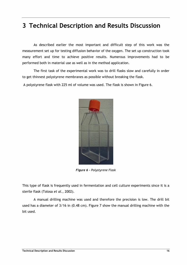
A polystyrene flask with 225 ml of volume was used. The flask is shown in Figure 6.

Figure 6 - Polystyrene Flask

This type of flask is frequently used in fermentation and cell culture experiments since it is a

sterile flask (Tolosa et al., 2002).

A manual drilling machine was used and therefore the precision is low. The drill bit

used has a diameter of 3/16 in (0.48 cm). Figure 7 show the manual drilling machine with the

bit used.


Figure 7 - Manual drilling machine with drill bit

After drilling, the membrane was cut out from the flask with a sharp tool. Representative

shape of the membrane is shown in Figure 8.

Figure 8 - Illustrative example of the polystyrene membrane shape

Since the mill bit used to drill the flask is not flat, the resulting membrane is also not

flat.

As the membrane is not flat a profile study must be performed. To do such a study

several marks on centre and with 1 mm of distance between them were made in the

polystyrene membrane, as the vertical lines of Figure 8 indicate. After measure the mark’s

thickness with a micrometer in ten samples, a graphic with the average thickness values was

build. The membrane profile study is shown on Figure 9.


Figure 9 - Polystyrene membrane profile

The length of the membrane from the center, expressed as zero in the abscissa plot,

until one peripheries side of the membrane express in the abscissa axis as a 0.3 is represented

in Figure 9. Only half of the membrane measurements were shown, as the membrane exhibit

rotational symmetry due to the manufacturing method.

Figure 9 shows that the thickest point is at the centre of the membrane while the

thinnest point is at the periphery of the membrane. At the centre the average thickness is

0.5473 mm (547.3 µm) and in the closest point of the periphery is 0.1796 mm (179.6 µm).

Once the membrane profile is known the oxygen sensor can be made. The procedure

for designing the oxygen sensor is described in Annex 1. When the sensor was ready it was

positioned above the membrane.

Since this study is focused in unidirectional diffusion the sensor must be encapsulated to

avoid side diffusion, making all the other sides impermeable to the oxygen like is shown in

Figure 10. The arrows depict the direction of the diffusion.

Sensor

Optical Adhesive

Polystyrene

Figure 10 - Polystyrene membrane with encapsulate sensor

0.0

0.1

0.2

0.3

0.4

0.5

0.6

0 0.05 0.1 0.15 0.2 0.25 0.3 0.35

Thic

kness

(m

m)

Length (mm)


The material used to encapsulate the sensor was optical adhesive.

The optical adhesive used is clear and colorless to let the light reach the sensor. The

only requirement, after the application of the optical adhesive, is an ultraviolet light (UV)

cure. The UV cure is generally obtained in two steps: the precure, when the sample has an

uniform and short exposure; the second step is a longer cure or fully cure to guarantee a full

cross linking. The cure time also depends on the thickness and on the ultraviolet energy

applied. Nevertheless a precure time and full cure of 10 seconds and 5 to 10 minutes,

respectively is usually required (Norland, 2010). The precure is used to better set up the

sample, however in this case the sensor is under the optical adhesive so the precure it is not

necessary. A cure time of 6 minutes was used in this study.

After placing the sensor in the membrane and after encapsulation the measurements start.

To measure, the sensor was placed inside a glass flask. The flask has a cork with two

holes: one to let the nitrogen/air in and another to let the gases out. One tube connects the

flask with the nitrogen and air supplies. Nitrogen is commonly used in this type of study since

it is heavier than oxygen. When nitrogen is pumped into the flask, the oxygen is dragged out

of the flask. The glass flask was located above the fluorometer with the sensor inside the

flask. The sensor face that is not in contact with the membrane is turned to the fluorometer.

Readings started and when the system stabilizes, nitrogen was pumped into the flask

until it stabilizes again. Then oxygen is pumped into the flask until it stabilizes again. Gases

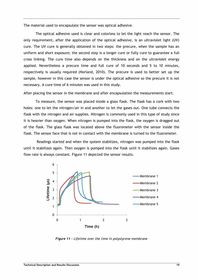
flow rate is always constant. Figure 11 depicted the sensor results.

Figure 11 - Lifetime over the time in polystyrene membrane

0

1

2

3

4

5

6

0 1 2 3

Lif

eti

me (

µs)

Time (h)

Membrane 1

Membrane 2

Membrane 3

Membrane 4

Membrane 5


Analyzing the Figure 11 it is visible that, once the nitrogen is pumped, the value of

lifetime increases. Lifetime starts to decrease, when oxygen is pumped into the flask due the

dynamic quenching, that was already explained before. Membrane two has a faster response

time because the encapsulation is imperfect, allowing direct gas entrance through cracks and

consequently response time decreases. The same thing happens in membrane 1 and 5

however the response time is slower because there are not so much cracks. In the other hand

membranes four and five have the slowest response time. This happens because some optical

adhesive leak into the sensor and block some fluorometer light increase the response the

response time. Nevertheless the response time of the membranes was around one hour. The

difference between the lifetimes can be explained by the lack of homogeneity in the sensor.

Despite of the fact that good encapsulation was very hard to achieve, the membranes give an

approximation of the response time expected.

When the membrane measurements were finished, flasks with a built in sensor became

experimental objects. Before the measurement the polystyrene flask has to be drilled and the

sensor placed in the cavity. Figure 12 illustrate the final look of the polystyrene flask.

Optical Adhesive

Figure 12 - Flask cross section for optical adhesive experiment

Optical adhesive is used again to encapsulate the sensor. For pumping nitrogen and

air, the same tube and cork from the previous experiment were used as both flasks have the

same diameter. This cork was used in all the following experiments. Once again the sensor

face that is not in contact with the polystyrene was placed on the fluorometer. The

measurement procedure is the same as for the membranes. Flask’s results are depicted in

Figure 13.

Sensor

Polystyrene


Figure 13 - Lifetime over time in flask

The curves depicted in Figure 13 show that again results are very different. The

explanations for such different curves are the same as with the membranes. However this

experiment shows that the response time in flasks is higher. This can be explained by the

superior thickness of the flask membrane compare with the single membrane. The

measurement of the flask membrane was very difficult to accomplish. In order to measure the

flask membrane thickness it was necessary to break the flask to remove the membrane.

However the membrane was glued in the encapsulated material, making the removal of the

membrane very hard to do without breaking it. Another problem faced was the slight

irregularly of the wall flask, therefore measuring the wall thickness and subtract the depth

drill gave an inaccuracy value. However this method was used to give an approximate value of

the flask membrane. The average wall thickness of the flask is 1.7 mm.

Drilling changed radically with the CNC milling machine arrival. This machine was much

more precise that the previous one due the computing control. With this machine feed rate,

speed rate and mill bit position was controlled with high accuracy. Though, in order to

control all this parameters it was necessary to write a specific code. That code is termed G-

code. The drill bit used has 3/16 in (0.48 cm) of diameter, the same dimensions that the drill

bit used before. CNC milling machine is illustrated in Figure 14.

0

1

2

3

4

5

6

0 1 2 3 4 5 6

Lif

eti

me (

µs)

Time (h)

Cavity A

Cavity B

Cavity C

Cavity D

Cavity E


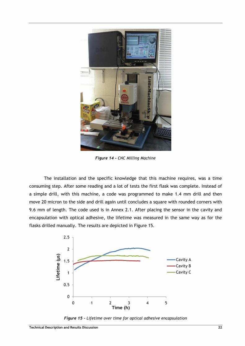
Figure 14 - CNC Milling Machine

The installation and the specific knowledge that this machine requires, was a time

consuming step. After some reading and a lot of tests the first flask was complete. Instead of

a simple drill, with this machine, a code was programmed to make 1.4 mm drill and then

move 20 micron to the side and drill again until concludes a square with rounded corners with

9.6 mm of length. The code used is in Annex 2.1. After placing the sensor in the cavity and

encapsulation with optical adhesive, the lifetime was measured in the same way as for the

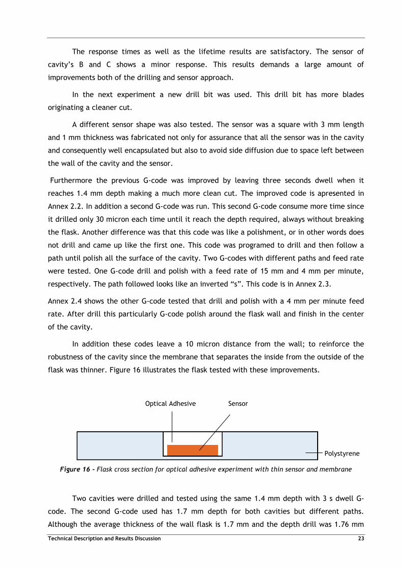
flasks drilled manually. The results are depicted in Figure 15.

Figure 15 - Lifetime over time for optical adhesive encapsulation

0

0.5

1

1.5

2

2.5

0 1 2 3 4 5

Lif

eti

me (

µs)

Time (h)

Cavity A

Cavity B

Cavity C


The response times as well as the lifetime results are satisfactory. The sensor of

cavity’s B and C shows a minor response. This results demands a large amount of

improvements both of the drilling and sensor approach.

In the next experiment a new drill bit was used. This drill bit has more blades

originating a cleaner cut.

A different sensor shape was also tested. The sensor was a square with 3 mm length

and 1 mm thickness was fabricated not only for assurance that all the sensor was in the cavity

and consequently well encapsulated but also to avoid side diffusion due to space left between

the wall of the cavity and the sensor.

Furthermore the previous G-code was improved by leaving three seconds dwell when it

reaches 1.4 mm depth making a much more clean cut. The improved code is apresented in

Annex 2.2. In addition a second G-code was run. This second G-code consume more time since

it drilled only 30 micron each time until it reach the depth required, always without breaking

the flask. Another difference was that this code was like a polishment, or in other words does

not drill and came up like the first one. This code was programed to drill and then follow a

path until polish all the surface of the cavity. Two G-codes with different paths and feed rate

were tested. One G-code drill and polish with a feed rate of 15 mm and 4 mm per minute,

respectively. The path followed looks like an inverted “s”. This code is in Annex 2.3.

Annex 2.4 shows the other G-code tested that drill and polish with a 4 mm per minute feed

rate. After drill this particularly G-code polish around the flask wall and finish in the center

of the cavity.

In addition these codes leave a 10 micron distance from the wall; to reinforce the

robustness of the cavity since the membrane that separates the inside from the outside of the

flask was thinner. Figure 16 illustrates the flask tested with these improvements.

Optical Adhesive Sensor

Polystyrene

Figure 16 - Flask cross section for optical adhesive experiment with thin sensor and membrane

Two cavities were drilled and tested using the same 1.4 mm depth with 3 s dwell G-

code. The second G-code used has 1.7 mm depth for both cavities but different paths.

Although the average thickness of the wall flask is 1.7 mm and the depth drill was 1.76 mm


too, it is simple to understand that when the drill bit touches the polystyrene flask surface a

force is applied. When the code start to drill that force is higher and therefore bends the

polystyrene flask. The programmed depth does not correspond to the real depth drill.

These results are depicted in Figure 17.

Figure 17 - Lifetime for optical adhesive encapsulation, thin sensor and membrane

In the cavity “A” the 1.76 mm depth with 10 micron side and side to the center path

G-code was used. In the other hand the 1.76 mm depth with 10 micron side and inverted “s”

path G-code was used in cavity “B”. It seems that the cavity “A” has a shorter response time.

Nevertheless the results are still not as good as expected and for some reason, that is not

possible to explain now, the sensor does not response when oxygen is blowing into the flask.

For this reason a new encapsulation material and approach was tested.

The selected material was the silicone with a piece of glass glue in the flask, also with

silicone, to seal the cavity.

Figure 18 illustrated the cross section of the flask.

Silicone Sensor

Glass

Polystyrene

Figure 18 - Flask cross section for silicone encapsulation

0

1

2

3

4

5

6

0 1 2 3 4 5 6

Lif

eti

me (

µs)

Time (h)

Cavity A

Cavity B


The results of the test of two samples with 1.73 mm depth cavities are depicted in

Figure 19.

Figure 19 - Lifetime for silicone encapsulation

The response time were around five hours but for the first time the experimental

curves were similar to the theoretical ones and to the ones made with the manual drilling

machine. This results show that the drilling must be improved in order to decrease the

response time. The results were satisfactory (except for the response time) and an

experiment with a cell culture inside the flask was tested. A brand new flask has to be drilled

to assure that the flask was sterile. The 1.73 mm depth G-code was maintained. Furthermore

a patch with the same features as the sensor used was placed inside the flask to monitor the

oxygen consumed by the cells, in situ, to verified if sensor measurement is the same as patch

measurement. Two coasters were used to measure the lifetime, one for the sensor and

another for the patch. The flask and the coasters were located inside an incubator with 95%

of air and 5% of carbon dioxide. Cell density in the beginning and end of the experiment was 2

x 106 and 3.5 x 106, respectively. These are normal cell growth values (Vallejos et al., 2010).

Figure 20 illustrates the results of the silicone encapsulation with cell culture.

0

0.5

1

1.5

2

2.5

3

3.5

4

4.5

5

0 2 4 6 8 10 12

Lif

eti

me (

µs)

Time (h)

Cavity A

Cavity B


Figure 20 - Lifetime comparison between sensor and patch for silicone encapsulation and cell culture

As shown in Figure 20 the sensor does not respond. Nevertheless the patch measured

the lifetime of the sensor. The patch curve makes sense due the consumption of oxygen by

the cells. As explained before the growth of the cells is possible if oxygen is consumed.

Therefore the oxygen does not quench the RUDPP fluorescence and lifetime increase. When

the growth of the cells reaches the stationary phase the lifetime stabilizes. In death phase

the lifetime will decrease since the cells do not consume oxygen leaving this gas free to

quench the fluorescence of the RUDPP. In Figure 20 does not appear this latter phase because

the experiment was stopped before since the sensor did not respond. A possible explanation

could be the side diffusion that occurs in silicone used to glue the glass in the polystyrene

flask. To prevent that, polyacrylonitrile, PAN, dissolved in n,n-dimethylformamide, DMF, was

used to seal the glass. Pan is a well known synthetic resin for the low permeability to gases

(Britannica, 2010). For this experiment a 1.76 mm depth drill and no patch was used. The

results are presented in Figure 21.

0

0.5

1

1.5

2

2.5

3

3.5

4

0 20 40 60 80

Lif

eti

me (

µs)

Time (h)

Patch

Sensor


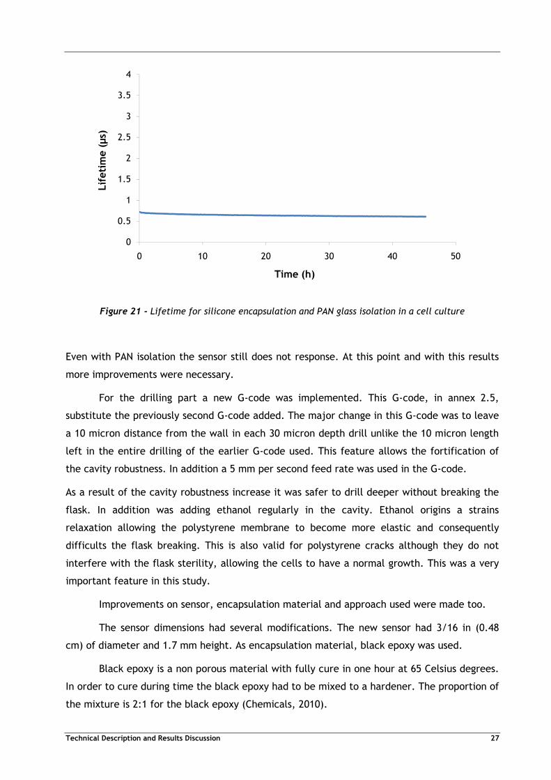
Figure 21 - Lifetime for silicone encapsulation and PAN glass isolation in a cell culture

Even with PAN isolation the sensor still does not response. At this point and with this results

more improvements were necessary.

For the drilling part a new G-code was implemented. This G-code, in annex 2.5,

substitute the previously second G-code added. The major change in this G-code was to leave

a 10 micron distance from the wall in each 30 micron depth drill unlike the 10 micron length

left in the entire drilling of the earlier G-code used. This feature allows the fortification of

the cavity robustness. In addition a 5 mm per second feed rate was used in the G-code.

As a result of the cavity robustness increase it was safer to drill deeper without breaking the

flask. In addition was adding ethanol regularly in the cavity. Ethanol origins a strains

relaxation allowing the polystyrene membrane to become more elastic and consequently

difficults the flask breaking. This is also valid for polystyrene cracks although they do not

interfere with the flask sterility, allowing the cells to have a normal growth. This was a very

important feature in this study.

Improvements on sensor, encapsulation material and approach used were made too.

The sensor dimensions had several modifications. The new sensor had 3/16 in (0.48

cm) of diameter and 1.7 mm height. As encapsulation material, black epoxy was used.

Black epoxy is a non porous material with fully cure in one hour at 65 Celsius degrees.

In order to cure during time the black epoxy had to be mixed to a hardener. The proportion of

the mixture is 2:1 for the black epoxy (Chemicals, 2010).

0

0.5

1

1.5

2

2.5

3

3.5

4

0 10 20 30 40 50

Lif

eti

me (

µs)

Time (h)


In addition to seal the cavity a Poly(methyl methacrylate) (PMMA) plate was used. The PMMA

plate is depicted in Figure 22.

Figure 22 - PMMA plate

In Figure 22 the black lines correspond to the PMMA plate shape. The grey line and the orange

line are for illustrated the cavity and the sensor, respectively. One hole of the PMMA plate is

to introduce the encapsulation material with the help of a syringe. In the second hole is

placed another syringe to suck the material. In this way it is guaranteed that the

encapsulation material will surround the sensor and fill the rest of the cavity without air

bubbles. The PMMA plate has a 1.3 cm length and the holes have 4 mm diameter. This PMMA

plate as well as the method to apply the encapsulation material was used in all the

experiments reported in the following text.

Figure 23 show the flask with these modifications.

PMMA Plate Sensor Black Epoxy

Polystyrene

Figure 23 - Cross section for black epoxy encapsulation

The results for these improvements were depicted in Figure 24.


Figure 24 - Lifetime for black epoxy encapsulation

Once again the sensor did not respond. In the next experiment the black epoxy was

used again but with a polyvinyl alcohol, PVA, treatment before.

The cavity was previously filled with a 1% PVA aqueous solution. Then the flask is

placed in the vacuum at 2 bar and 65 Celsius degrees and left there overnight to make sure

that all the water was evaporated. When the solution dries a thin layer of PVA stays in the

cavity. Figure 25 illustrates the results.

Figure 25 - Lifetime for PVA and black epoxy encapsulation

0

0.5

1

1.5

2

2.5

3

3.5

4

0 5 10 15 20

Lif

eti

me (

µs)

Time (h)

0.0

0.5

1.0

1.5

2.0

2.5

3.0

3.5

4.0

0 0.2 0.4 0.6 0.8 1

Lif

eti

me (

µs)

Time (h)

Cavity A

Cavity B


The sensor one more time did not respond. The reason of this phenomenon is probably

because black epoxy leaks into the sensor blocking the coaster light and resulting in a stable

lifetime.

For the next experiment an epoxy resin was used to encapsulate the sensor. The epoxy

resin had to be mix with a hardener in a 100:15 proportion. This mixture is appropriate for

low fluorescence applications and has a fast full cure time, only one hour at 65 Celsius

degrees (Andover, 2010). Graphite was also added. The graphite was added because the

epoxy has some fluorescence. Since the graphite had a dark color, the fluorescence is blocked

because the light is not reflected to the photodetector and therefore only the sensor

fluorescence is measured. The addition of the graphite was made before the hardener to

avoid the cure before the material application.

Although the epoxy was very promising material, the fast cure does not let time to

properly mix it with the hardener and introduce the mixture into the cavity without

solidifying.

Therefore another epoxy and hardener were used keeping all the other parameters

equal. This new epoxy has a long full cure time, between 12 and 24 hours at 25 Celsius

degrees, therefore the application of the material could be done (Elmer's, 2010). The results

are depicted in Figure 26.

Figure 26 - Lifetime for epoxy encapsulation

For the epoxy encapsulation the results do not have explanation at this moment. Hence the

sensor does not respond the way it should thus it is necessary to change the encapsulation

material.

-25

-20

-15

-10

-5

0

5

10

0 0.02 0.04 0.06 0.08 0.1

Lif

eti

me (

µs)

Time (h)


The new encapsulation material tested was a resin.

The resin needs a catalyst to fully cure. The amount of catalyst used depends on the

quantity of resin as well as on the thickness that the application needs (Castin'Craft, 2010).

Once again graphite was used to avoid the resin fluorescence interfere with the sensor

fluorescence measurement.

In this set of experiments three tests were performed in different days. The second

measurement was made three days after the first measurement. The third measurement was

made seven days after the first one. This tests was only conducted with nitrogen in.

Figure 27 illustrate the results.

Figure 27 - Lifetime for resin encapsulation

With the resin encapsulation the first measurement does not exhibit good results,

although after three days the second measurement indicates promising results. This

measurement has a faster response time and promise good results for the next measurement.

Nevertheless after seven days, a fully cure resin revealed the true lifetime of the resin. The

first and second measurement curves could be explained by a not complete bonding of the

molecules.

For the next experiment another encapsulation material was used. This time the

material used was something completely different.

0

1

2

3

4

5

6

7

0 1 2 3 4 5 6 7

Lif

eti

me (

µs)

Time (h)

First Measurement

Second Measurement

Third Measurement


Bismuth alloy or more commonly Wood’s alloy is a fusible alloy. This alloy is a mixture

of 50% bismuth, 25% lead, 12.5% tin, and 12.5% cadmium. However the major feature of this

alloy is the low melting point, only 70 Celsius degrees (Reade, 2010). The principal

component of this alloy is the bismuth. This particular alloy is capable to expand if it exists in

proportions equal or higher than 50%. If the proportion of bismuth is lower than 50% this alloy

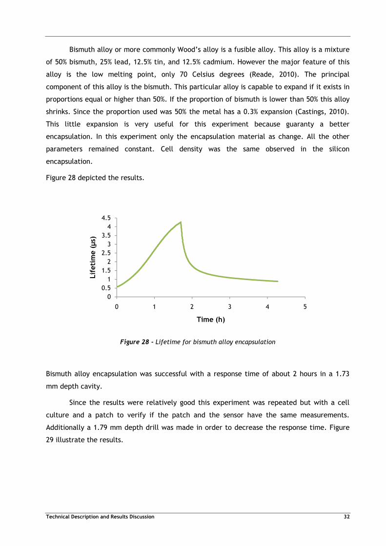
shrinks. Since the proportion used was 50% the metal has a 0.3% expansion (Castings, 2010).

This little expansion is very useful for this experiment because guaranty a better

encapsulation. In this experiment only the encapsulation material as change. All the other

parameters remained constant. Cell density was the same observed in the silicon

encapsulation.

Figure 28 depicted the results.

Figure 28 - Lifetime for bismuth alloy encapsulation

Bismuth alloy encapsulation was successful with a response time of about 2 hours in a 1.73

mm depth cavity.

Since the results were relatively good this experiment was repeated but with a cell

culture and a patch to verify if the patch and the sensor have the same measurements.

Additionally a 1.79 mm depth drill was made in order to decrease the response time. Figure

29 illustrate the results.

0

0.5

1

1.5

2

2.5

3

3.5

4

4.5

0 1 2 3 4 5

Lif

eti

me (

µs)

Time (h)


Figure 29 - Lifetime comparison between sensor and patch for bismuth alloy encapsulation with cell

culture

The results were a little different. The patch has the expected curve already discuss earlier.

The sensor does not response, until the exponential phase but after that phase the sensor

have a behavior similar to the patch. The reason for the initial response delay was some little

air bubbles existence that interferes with the coaster measurements. After the cells start

consuming the oxygen, the air bubbles disappear and the coaster start to read with more

accuracy. Although the curves does not match, this experiment was successful because verify

that the sensor could measure the lifetime through one thin polystyrene membrane.

Another experiment was made in order to decrease the response time and avoid the

air bubbles. Bismuth alloy was once again used but before the encapsulation with this alloy

the cavity was filled with the hardener and then leaves it dry. The hardener addition was for

originate micro cracks for oxygen diffuse faster and consequently decrease the initial delay

observed in the previous experiment. In this experiment only nitrogen was blowing into the

flask. The cavity has 1.73 mm depth. The result is illustrated in Figure 30.

0

0.5

1

1.5

2

2.5

3

3.5

4

4.5

5

0 20 40 60 80 100 120

Lif

eti

me (

µs)

Time (h)

Patch

Sensor


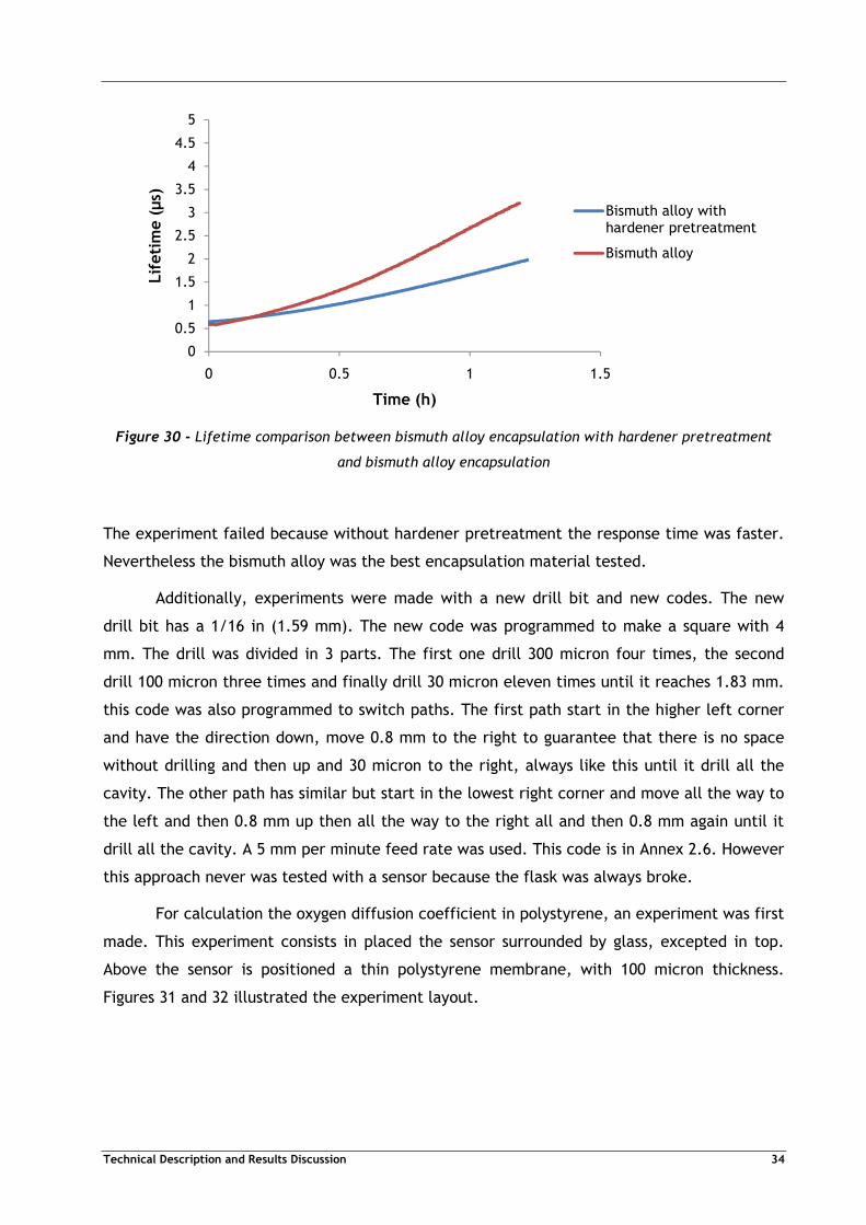
Figure 30 - Lifetime comparison between bismuth alloy encapsulation with hardener pretreatment

and bismuth alloy encapsulation

The experiment failed because without hardener pretreatment the response time was faster.

Nevertheless the bismuth alloy was the best encapsulation material tested.

Additionally, experiments were made with a new drill bit and new codes. The new

drill bit has a 1/16 in (1.59 mm). The new code was programmed to make a square with 4

mm. The drill was divided in 3 parts. The first one drill 300 micron four times, the second

drill 100 micron three times and finally drill 30 micron eleven times until it reaches 1.83 mm.

this code was also programmed to switch paths. The first path start in the higher left corner

and have the direction down, move 0.8 mm to the right to guarantee that there is no space

without drilling and then up and 30 micron to the right, always like this until it drill all the

cavity. The other path has similar but start in the lowest right corner and move all the way to

the left and then 0.8 mm up then all the way to the right all and then 0.8 mm again until it

drill all the cavity. A 5 mm per minute feed rate was used. This code is in Annex 2.6. However

this approach never was tested with a sensor because the flask was always broke.

For calculation the oxygen diffusion coefficient in polystyrene, an experiment was first

made. This experiment consists in placed the sensor surrounded by glass, excepted in top.

Above the sensor is positioned a thin polystyrene membrane, with 100 micron thickness.

Figures 31 and 32 illustrated the experiment layout.

0

0.5

1

1.5

2

2.5

3

3.5

4

4.5

5

0 0.5 1 1.5

Lif

eti

me (

µs)

Time (h)

Bismuth alloy with hardener pretreatment

Bismuth alloy


Polystyrene membrane Sensor Silicone

Glass

Figure 31 - Oxygen diffusion coefficient in polystyrene testing scheme

Polystyrene membrane

Sensor

Silicone

Glass

Figure 32 – Top view scheme

Then this set up was placed inside a Petri’s box and properly sealed with parafilm. Then

needles connected with air and nitrogen supplies were introduced in the system.

Results are depicted in Figure 33.

Figure 33 - Lifetime for silicone encapsulation in glass

0

0.5

1

1.5

2

2.5

3

3.5

4

0 1 2 3 4 5 6 7

Lif

eti

me (

µs)

Time (h)


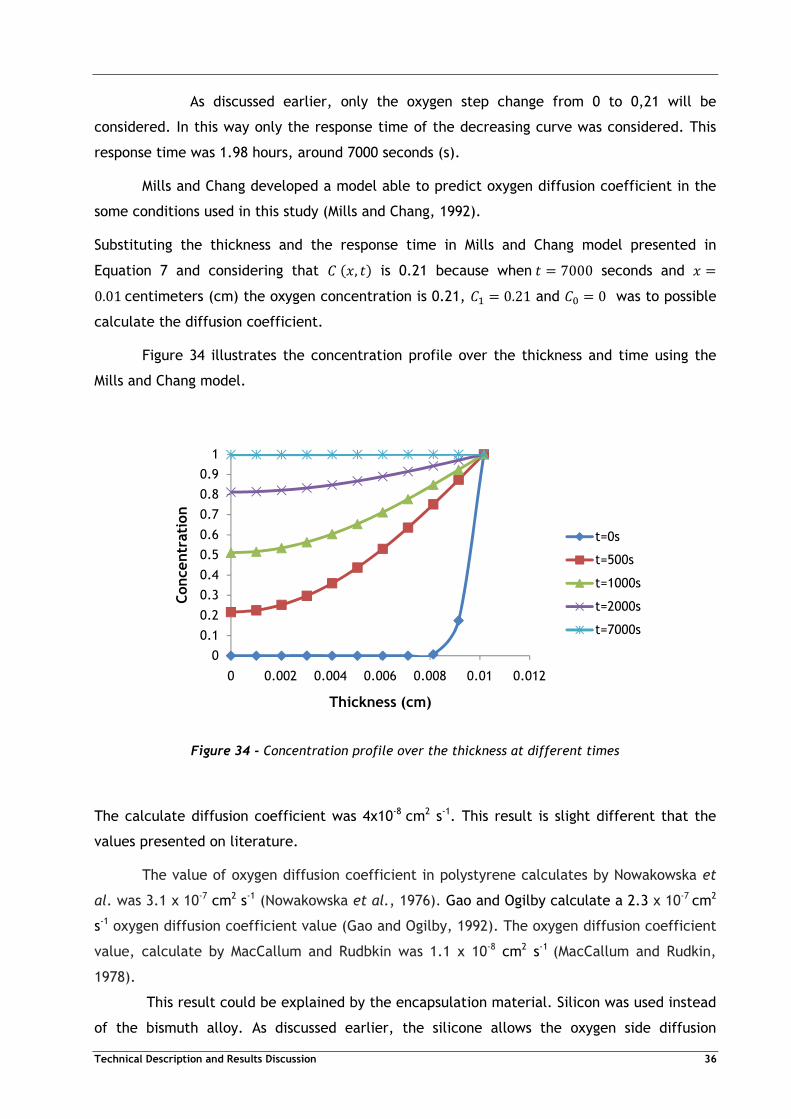
As discussed earlier, only the oxygen step change from 0 to 0,21 will be

considered. In this way only the response time of the decreasing curve was considered. This

response time was 1.98 hours, around 7000 seconds (s).

Mills and Chang developed a model able to predict oxygen diffusion coefficient in the

some conditions used in this study (Mills and Chang, 1992).

Substituting the thickness and the response time in Mills and Chang model presented in

Equation 7 and considering that � !�, �" is 0.21 because when � � 7000 seconds and � �0.01 centimeters (cm) the oxygen concentration is 0.21, �� 0.21 and �� 0 was to possible

calculate the diffusion coefficient.

Figure 34 illustrates the concentration profile over the thickness and time using the

Mills and Chang model.

Figure 34 - Concentration profile over the thickness at different times

The calculate diffusion coefficient was 4x10-8 cm2 s-1. This result is slight different that the

values presented on literature.

The value of oxygen diffusion coefficient in polystyrene calculates by Nowakowska et

al. was 3.1 x 10-7 cm2 s-1 (Nowakowska et al., 1976). Gao and Ogilby calculate a 2.3 x 10-7 cm2

s-1 oxygen diffusion coefficient value (Gao and Ogilby, 1992). The oxygen diffusion coefficient

value, calculate by MacCallum and Rudbkin was 1.1 x 10-8 cm2 s-1 (MacCallum and Rudkin,

1978).

This result could be explained by the encapsulation material. Silicon was used instead

of the bismuth alloy. As discussed earlier, the silicone allows the oxygen side diffusion

0

0.1

0.2

0.3

0.4

0.5

0.6

0.7

0.8

0.9

1

0 0.002 0.004 0.006 0.008 0.01 0.012

Concentr

ati

on

Thickness (cm)

t=0s

t=500s

t=1000s

t=2000s

t=7000s


interfering with the optical measurements. Furthermore different grades of polystyrene and

manufacturing processes as well as the length of the polymer chain introduce some variation

in the oxygen diffusion coefficient in polystyrene.

Conclusions 38

4 Conclusions

A new method for oxygen monitoring in polystyrene flasks was studied in the present

work. Using the fabrication methods developed in this study, it was proved to be possible to

monitor the oxygen concentration while maintaining the original sterility of the flask with a

100 micron thick polystyrene membrane.

For sensing oxygen through a thin polystyrene membrane, the back and side of the

membrane have to be isolated from the oxygen.

In several encapsulation materials tested, the bismuth alloy was the best material for

encapsulation.

In this study was discover that ethanol origins a strains relaxation increasing the

elasticity of the polystyrene membrane.

Finally, the diffusion coefficient of oxygen through the material of the flask was

calculated as 4x10-8cm2 s-1.

Certainly this study will be helpful in future oxygen concentration studies with cell

cultures.

Work Evaluation 39

5 Work Evaluation

5.1 Accomplish Goals

This study successfully proves that the oxygen sensor can be positioned in the external

surface of the flask. A technique to drill deeper and consequently decrease the polystyrene

membrane and the response time was developed with the CNC milling machine with the

addition of ethanol. The drilling technique does not compromise the flask sterility.

Different encapsulation materials were used although none of the several materials

studies accomplished 100% its function. The bismuth alloy present reasonably results.

The oxygen diffusion coefficient of oxygen in polystyrene was obtained.

The mathematical model capable to predict the response time for oxygen

concentration and thickness variation was not created due the difficulty for measure the

membrane thickness.

5.2 Limitations and Future Improvements

The only and major limitation of this work was the flask’s wall thickness

measurement. For future studies a non invasive method to measure the wall thickness is

imperative. In order to accomplish the measurement inexpensively, ultrasounds and optical

measurements were necessary. Both techniques can measure with accuracy and most of all

with the precision required.

Ultrasonic technique use high frequency sound waves to measure thickness. To achieve

precise measurement, usually a frequency between 500 KHz and 100 KHz is used ( Fowler,

1997). In order to measure, electrical pulses excite transducers that generate sound waves.

Each material has it’s own acoustic characteristic. To fulfill all that wide range, transducers

are being developed.

Thickness can be determined by measuring the necessary time that the sound wave,

generated by the transducer, takes to travel through the sample thickness, reflect and

returned to the transducer (Fowler, 1997). Using Equation (9) it is possible to obtain the

thickness.

Work Evaluation 40

� � � �2 (9)

where � is the thickness, � is the velocity of sound waves in the material and � the time. As

the sound waves go and come the time has to be divided by 2.

Optical measurement method is similar to the ultrasonic technique but with light

emission instead of the sound waves.

As encapsulation material, bismuth alloy presents reasonably results. However it is

necessary to continue research on the development of different methods for encapsulation.

The drilling part still has also to be improved. A 100 micron thickness membrane

without compromising the flask sterility is a remarkable result but it is still not sufficient for

acceptable response times.

5.3 Final Appreciation

I really enjoyed the time spend developing this study. I learned and also worked a lot

in order to accomplish the objectives initially propose. However I believe that this was a very

ambitious work for the time available to do it. With time and some improvements, this study

will definitely be the basis for an improvement in cells culture oxygen monitorization.

References 41

6 References

Andover. (2010). "Epolite FH-5313 Epoxy." Retrieved July 5, 2010, from http://www.andovercorp.com/web_store/pdf/Catalog/Sections/Andover_Epoxy.pdf.

Britannica, E. (2010). "Human Genetics." Retrieved July 4, 2010, from http://www.britannica.com/EBchecked/topic/228983/human-genetics/50734/The-genetics-of-antibody-formation?anchor=ref502673.

Britannica, E. (2010). "Monoclonal antibody." Retrieved July 4, 2010, from http://www.britannica.com/EBchecked/topic/389772/monoclonal-antibody/214785/Hybridoma.

Britannica, E. (2010). "Polyacrylonitrile." Retrieved June 4, 2010, from http://www.britannica.com/EBchecked/topic/468259/polyacrylonitrile.

Castin'Craft. (2010). "Casting Resin." Retrieved July 5, 2010, from http://www.eti-usa.com/consum/castresn/castinst.htm.

Castings, A. (2010). "Fusible alloys." Retrieved July 5, 2010, from http://www.alchemycastings.com/lead-products/fusible.htm.

Chasteen, T. G. (1996). "Jablonski Diagram." Retrieved June 20, 2010, from http://elchem.kaist.ac.kr/vt/chem-ed/quantum/graphics/jablon.gif.

Chemicals, M. (2010). "Black epoxy." Retrieved July 5, 2010, from http://www.mgchemicals.com/products/832b.html.

Cox, M. E. and Dunn, B. (1986). "Oxygen diffusion in poly(dimethyl siloxane) using fluorescence quenching. I. Measurement technique and analysis." Journal of Polymer Science Part A: Polymer Chemistry 24(4): 621-636.

Cox, M. E. and Dunn, B. (1986). "Oxygen diffusion in poly(dimethyl siloxane) using fluorescence quenching. II. Filled samples." Journal of Polymer Science Part A: Polymer Chemistry 24(10): 2395-2400.

Czarnecki, S. and Kryszewski, M. (1963). "Some applications of afterglow studies of luminescent compounds in solid polymers." Journal of Polymer Science Part A: General Papers 1(10): 3067-3077.

Decker, J. (2005). Retrieved July 4, 2010, from http://www.microvet.arizona.edu/Courses/MIC205/Exams/05Exams/05Ex2key.htm.

Demas, J. N.; DeGraff, B. A.; Xu, W.(1995). "Modeling of Luminescence Quenching-Based Sensors: Comparison of Multisite and Nonlinear Gas Solubility Models." Analytical Chemistry 67(8): 1377-1380.

Elmer's. (2010). "Epoxy cement." Retrieved July 5, 2010, from http://www.elmers.com/product/detail/E1009?filterPath=epoxy.

Gao, Y. and Ogilby, P. R. (1992). "A new technique to quantify oxygen diffusion in polymer films." Macromolecules 25(19): 4962-4966.

Guillet, J. E. and Andrews, M. (1992). "Studies of oxygen diffusion in poly(styrene-co-1-naphthyl methacrylate) by phosphorescence quenching." Macromolecules 25(10): 2752-2756.

Gupta, A. and Rao, G. (2003). "A study of oxygen transfer in shake flasks using a non-invasive oxygen sensor." Biotechnology and Bioengineering 84(3): 351-358.

References 42

Holland, R. V.; Rooney, M. L.; Santangelo, R. A. (1980). "Measuring oxygen permeabilities of polymer films by a new singlet oxygen technique." Angewandte Makromolekulare Chemie 88(1): 209-221.

Hormats, E. I. and Unterleitner, F. C. (1965). "Measurement of the Diffusion of Oxygen in Polymers by Phosphorescent Quenching1." The Journal of Physical Chemistry 69(11): 3677-3681.

Fowler, K. A.; Elfbaum, G. M.; Smith, K. A.; Nelligan, T. J. (1997). "Theory and application of precision ultrasonic thickness gaging." Retrieved July 6, 2010, from http://www.ndt.net/article/wt1097/panam/panam.htm#1.

Kneas, K. A.; Demas, J. N.; Nguyen, B.; Lockhart, A.; Xu, W.; DeGraff, B. A. (2002). "Method for Measuring Oxygen Diffusion Coefficients of Polymer Films by Luminescence Quenching." Anal. Chem. 74: 1111-1118.

Kocincova, A. S.; Borisov, S. M.; Krause, Christian.; Wolfbeis, O. S. (2007). "Fiber-optic microsensors for simultaneous sensing of oxygen and pH, and of oxygen and temperature." Anal Chem 79(22): 8486-8493.

Lakowicz, J. R. (2006). Principles of fluorescence spectroscopy. New York, Springer.

Lu, L. and Weiss, R. G. (1994). "Insights into the mechanism of diffusion of some N,N-dialkylanilines in "native" low density polyethylene films using a simple fluorescence technique." Macromolecules 27(1): 219-225.

MacCallum, J. R. and Rudkin, A. L. (1978). "A novel technique for measuring TH diffusion constant of oxygen in polymer films." European Polymer Journal 14(9): 655-656.

Mills, A. and Chang, Q. (1992). "Modelled diffusion-controlled response and recovery behaviour of a naked optical film sensor with a hyperbolic-type response to analyte concentration." Analyst 117: 1461-1466.

Norland. (2010). "Optical Adhesive 61." Retrieved June 21, 2010, from http://www.norlandprod.com/adhesives/noa%2061.html.

Nowakowska, M.; Najbar,J .; Waligóra, B. (1976). "Fluorescence quenching of polystyrene by oxygen." Eur. Polym. J. 12: 387-391.

Oxford, R. O. (2010). "Elastomer." Retrieved July 10, 2010, from https://vpn.umbc.edu/views/,DanaInfo=www.oxfordreference.com+ENTRY.html?entry=t81.e1465&srn=1&ssid=90455805#FIRSTHIT

Oxford, R. O. (2010). "Hybridoma." Retrieved July 4, 2010, from https://vpn.umbc.edu/views/,DanaInfo=www.oxfordreference.com+SEARCH_RESULTS.html?q=hybridomas&authstatuscode=202&ssid=695507364&time=0.317485286185718.

Oxford, R. O. (2010). "Luminescence." Retrieved July 2, 2010, from https://vpn.umbc.edu/views/,DanaInfo=www.oxfordreference.com+ENTRY.html?entry=t224.e3663&srn=2&ssid=1015451574#FIRSTHIT

Oxford, R. O. (2010). "Singlet." Retrieved July 26, 2010, from https://vpn.umbc.edu/views/,DanaInfo=www.oxfordreference.com+ENTRY.html?entry=t81.e3747&srn=1&ssid=348528699#FIRSTHIT.

Oxford, R. O. (2010). "Triplet." Retrieved July 26, 2010, from https://vpn.umbc.edu/views/,DanaInfo=www.oxfordreference.com+ENTRY.html?entry=t81.e4185&srn=2&ssid=376281312#FIRSTHIT.

Petrak, K. (1979). "Permeability of oxygen through polymers. I. A novel spectrophotochemical method." Journal of Applied Polymer Science 23(8): 2365-2371.

Randers-Eichhorn, L.; Bartlett,R. A.; Frey, D.D.; Rao,G. (1996). "Noninvasive oxygen measurements and mass transfer considerations in tissue culture flasks." Biotechnology and Bioengineering 51(4): 466-478.

References 43

Reade. (2010). "Wood's alloy." Retrieved July 5, 2010, from http://www.reade.com/products/4-alloys-metal-inorganic-powder-sheet-a-wire/822-woods-metal-alloy-cerro-bend-onions-fusible-alloy-woods-metal-fusible-alloy-bismuthleadtincadmium-alloy-bendalloy-pewtalloy-sn-pb-bi-cd-lipowitzs-alloy-cas-8049-22-7.

Shaw, G. (1967). "Quenching by Oxygen Diffusion of Phosphorescence Emission of Aromatic Molecules in Polymethyl Methacrylate." Trans. Faraday Soc. 63: 2181-2189.

Sigma-Aldrich. (2010). "Tris(4,7-diphenyl-1,10-phenanthroline)ruthenium(II) dichloride complex." Retrieved June 10, 2010, from http://www.sigmaaldrich.com/catalog/ProductDetail.do?lang=en&N4=76886|FLUKA&N5=SEARCH_CONCAT_PNO|BRAND_KEY&F=SPEC.

Stevenson, C. S. (2005). Excimer. A Dictionary of Chemistry. Oxford, Oxford University Press.

Stokes, G. G. (1852). "On the change of refrangibility of light." Phil. Trans. R. Soc. London 142: 463–562.

Tolosa, L.; Kostov,Y.; Harms, P.; Rao, G. (2002). "Noninvasive measurement of dissolved oxygen in shake flasks." Biotechnology and Bioengineering 80(5): 594-597.

Tolosa, L.; Kostov,Y.; Rao, G. (2006). Fluorescence-Based Sensors for Bioprocess Monitoring. Fluorescence Sensors and Biosensors. R. B.Thompson, CRC: 416.

Vallejos, J. R.; Brorson, K. A.; Moreira, A. R.; Rao, G. (2010). "Dissolved oxygen and pH profile evolution after cryovial thaw and repeated cell passaging in a T-75 flask." Biotechnology and Bioengineering 105(6): 1040-1047.

Wen, W.-Y. (1993). "Motion of Sorbed Gases in Polymers. , 117-126." Chem. Soc. Rev 22: 117-126.

Yekta, A., Z.; Masoumi, Z.; Winnik, M. A. (1995). "Luminescence measurements of oxygen permeation and oxygen diffusion in thin polymer films." Canadian Journal of Chemistry 73: 2021-2029.

Experimental Procedure for Oxygen Sensor Fabrication 44

Annex 1 Experimental Procedure for Oxygen

Sensor Fabrication

Reactants

1 gram of Silicone

0.5 ml of Toluene

50 mg of the oxygen sensitive dye, ruthenium (II) tris (4,7-diphenyl-1,10-phenanthroline)

Chloride (RUDPP)

Material

Balance

Pipette

Petri box

Watch Glass

Spatula

Description

1. Measure, with spatula and balance’s help, 50 mg of RUDPP and put it in a

watch glass

2. Measure 1 gram of silicone and add it in the watch glass

3. With a pipette, measure 0.5 ml of toluene and add it in the mixture

4. Mix until the mixture becomes homogeneous

5. Apply and leave it in a dark place at a room temperature for at least 24 hours

G-codes 45

Annex 2 G-codes

2.1 1.4 mm depth

F400

M3 s200

G1 z-1.4 f5

G0 z1.9

G0 x0.2

G0 z0

G1 z-1.4 f5

G0 z1.9

G0 x0.4

G0 z0

G1 z-1.4 f5

G0 z1.9

G0 x0.6

G0 z0

G1 z-1.4 f5

G0 z1.9

G0 x0.8

G0 z0

G1 z-1.4 f5

G0 z1.9

G0 x1

G0 z0

G1 z-1.4 f5

G0 z1.9

G0 x1.2

G0 z0

G1 z-1.4 f5

G0 z1.9

G0 x1.4

G0 z0

G1 z-1.4 f5

G0 z1.9

G0 x1.6

G0 z0

G1 z-1.4 f5

G0 z1.9

G0 x1.8

G0 z0

G1 z-1.4 f5

G0 z1.9

G0 x2

G0 z0

G1 z-1.4 f5

G0 z1.9

G0 x2.2

G0 z0

G1 z-1.4 f5

G0 z1.9

G0 x2.4

G0 z0

G1 z-1.4 f5

G0 z1.9

G0 x2.6

G0 z0

G1 z-1.4 f5

G0 z1.9

G0 x2.8

G0 z0

G1 z-1.4 f5

G0 z1.9

G0 x3

G0 z0

G1 z-1.4 f5

G0 z1.9

G0 x3.2

G0 z0

G1 z-1.4 f5

G0 z1.9

G0 x3.4

G0 z0

G1 z-1.4 f5

G0 z1.9

G0 x3.6

G0 z0

G1 z-1.4 f5

G0 z1.9

G0 x3.8

G0 z0

G1 z-1.4 f5

G0 z1.9

G0 x4

G0 z0

G1 z-1.4 f5

G0 z1.9

G0 x4.2

G0 z0

G1 z-1.4 f5

G0 z1.9

G0 x4.4

G0 z0

G1 z-1.4 f5

G0 z1.9

G0 x4.6

G0 z0

G1 z-1.4 f5

G0 z1.9

G0 x4.8

G0 z0

G1 z-1.4 f5

G0 z1.9

G0 y-0.2

G0 z0

G1 z-1.4 f5

G0 z1.9

G0 y-0.4

G0 z0

G1 z-1.4 f5

G0 z1.9

G0 y-0.6

G0 z0

G1 z-1.4 f5

G0 z1.9

G0 y-0.8

G0 z0

G1 z-1.4 f5

G0 z1.9

G0 y-1

G0 z0

G1 z-1.4 f5

G0 z1.9

G0 y-1.2

G0 z0

G1 z-1.4 f5

G0 z1.9

G0 y-1.4

G-codes 46

G0 z0

G1 z-1.4 f5

G0 z1.9

G0 y-1.6

G0 z0

G1 z-1.4 f5

G0 z1.9

G0 y-1.8

G0 z0

G1 z-1.4 f5

G0 z1.9

G0 y-2

G0 z0

G1 z-1.4 f5

G0 z1.9

G0 y-2.2

G0 z0

G1 z-1.4 f5

G0 z1.9

G0 y-2.4

G0 z0

G1 z-1.4 f5

G0 z1.9

G0 y-2.6

G0 z0

G1 z-1.4 f5

G0 z1.9

G0 y-2.8

G0 z0

G1 z-1.4 f5

G0 z1.9

G0 y-3

G0 z0

G1 z-1.4 f5

G0 z1.9

G0 y-3.2

G0 z0

G1 z-1.4 f5

G0 z1.9

G0 y-3.4

G0 z0

G1 z-1.4 f5

G0 z1.9

G0 y-3.6

G0 z0

G1 z-1.4 f5

G0 z1.9

G0 y-3.8

G0 z0

G1 z-1.4 f5

G0 z1.9

G0 y-4

G0 z0

G1 z-1.4 f5

G0 z1.9

G0 y-4.2

G0 z0

G1 z-1.4 f5

G0 z1.9

G0 y-4.4

G0 z0

G1 z-1.4 f5

G0 z1.9

G0 y-4.6

G0 z0

G1 z-1.4 f5

G0 z1.9

G0 y-4.8

G0 z0

G1 z-1.4 f5

G0 z1.9

G0 x4.6

G0 z0

G1 z-1.4 f5

G0 z1.9

G0 x4.4

G0 z0

G1 z-1.4 f5

G0 z1.9

G0 x4.2

G0 z0

G1 z-1.4 f5

G0 z1.9

G0 x4

G0 z0

G1 z-1.4 f5

G0 z1.9

G0 x3.8

G0 z0

G1 z-1.4 f5

G0 z1.9

G0 x3.6

G0 z0

G1 z-1.4 f5

G0 z1.9

G0 x3.4

G0 z0

G1 z-1.4 f5

G0 z1.9

G0 x3.2

G0 z0

G1 z-1.4 f5

G0 z1.9

G0 x3

G0 z0

G1 z-1.4 f5

G0 z1.9

G0 x2.8

G0 z0

G1 z-1.4 f5

G0 z1.9

G0 x2.6

G0 z0

G1 z-1.4 f5

G0 z1.9

G0 x2.4

G0 z0

G1 z-1.4 f5

G0 z1.9

G0 x2.2

G0 z0

G1 z-1.4 f5

G0 z1.9

G0 x2

G0 z0

G1 z-1.4 f5

G0 z1.9

G0 x1.8

G0 z0

G1 z-1.4 f5

G0 z1.9

G0 x1.6

G0 z0

G1 z-1.4 f5

G0 z1.9

G0 x1.4

G0 z0

G1 z-1.4 f5

G0 z1.9

G0 x1.2

G-codes 47

G0 z0

G1 z-1.4 f5

G0 z1.9

G0 x1

G0 z0

G1 z-1.4 f5

G0 z1.9

G0 x0.8

G0 z0

G1 z-1.4 f5

G0 z1.9

G0 x0.6

G0 z0

G1 z-1.4 f5

G0 z1.9

G0 x0.4

G0 z0

G1 z-1.4 f5

G0 z1.9

G0 x0.2

G0 z0

G1 z-1.4 f5

G0 z1.9

G0 x0

G0 z0

G1 z-1.4 f5

G0 z1.9

G0 y-4.6

G0 z0

G1 z-1.4 f5

G0 z1.9

G0 y-4.4

G0 z0

G1 z-1.4 f5

G0 z1.9

G0 y-4.2

G0 z0

G1 z-1.4 f5

G0 z1.9

G0 y-4

G0 z0

G1 z-1.4 f5

G0 z1.9

G0 y-3.8

G0 z0

G1 z-1.4 f5

G0 z1.9

G0 y-3.6

G0 z0

G1 z-1.4 f5

G0 z1.9

G0 y-3.4

G0 z0

G1 z-1.4 f5

G0 z1.9

G0 y-3.2

G0 z0

G1 z-1.4 f5

G0 z1.9

G0 y-3

G0 z0

G1 z-1.4 f5

G0 z1.9

G0 y-2.8

G0 z0

G1 z-1.4 f5

G0 z1.9

G0 y-2.6

G0 z0

G1 z-1.4 f5

G0 z1.9

G0 y-2.4

G0 z0

G1 z-1.4 f5

G0 z1.9

G0 y-2.2

G0 z0

G1 z-1.4 f5

G0 z1.9

G0 y-2

G0 z0

G1 z-1.4 f5

G0 z1.9

G0 y-1.8

G0 z0

G1 z-1.4 f5

G0 z1.9

G0 y-1.6

G0 z0

G1 z-1.4 f5

G0 z1.9

G0 y-1.4

G0 z0

G1 z-1.4 f5

G0 z1.9

G0 y-1.2

G0 z0

G1 z-1.4 f5

G0 z1.9

G0 y-1

G0 z0

G1 z-1.4 f5

G0 z1.9

G0 y-0.8

G0 z0

G1 z-1.4 f5

G0 z1.9

G0 y-0.6

G0 z0

G1 z-1.4 f5

G0 z1.9

G0 y-0.4

G0 z0

G1 z-1.4 f5

G0 z1.9

G0 y-0.2

G0 z0

G1 z-1.4 f5

G0 Z10

M30

G-codes 49

2.2 1.4 mm depth with 3 seconds dwell

F400

M3 s200

G1 z-1.4 f5

G4 P3

G0 z1.9

G0 x0.2

G0 z0

G1 z-1.4 f5

G4 P3

G0 z1.9

G0 x0.4

G0 z0

G1 z-1.4 f5

G4 P3

G0 z1.9

G0 x0.6

G0 z0

G1 z-1.4 f5

G4 P3

G0 z1.9

G0 x0.8

G0 z0

G1 z-1.4 f5

G4 P3

G0 z1.9

G0 x1

G0 z0

G1 z-1.4 f5

G4 P3

G0 z1.9

G0 x1.2

G0 z0

G1 z-1.4 f5

G4 P3

G0 z1.9

G0 x1.4

G0 z0

G1 z-1.4 f5

G4 P3

G0 z1.9

G0 x1.6

G0 z0

G1 z-1.4 f5

G4 P3

G0 z1.9

G0 x1.8

G0 z0

G1 z-1.4 f5

G4 P3

G0 z1.9

G0 x2

G0 z0

G1 z-1.4 f5

G4 P3

G0 z1.9

G0 x2.2

G0 z0

G1 z-1.4 f5

G4 P3

G0 z1.9

G0 x2.4

G0 z0

G1 z-1.4 f5

G4 P3

G0 z1.9

G0 x2.6

G0 z0

G1 z-1.4 f5

G4 P3

G0 z1.9

G0 x2.8

G0 z0

G1 z-1.4 f5

G4 P3

G0 z1.9

G0 x3

G0 z0

G1 z-1.4 f5

G4 P3

G0 z1.9

G0 x3.2

G0 z0

G1 z-1.4 f5

G4 P3

G0 z1.9

G0 x3.4

G0 z0

G1 z-1.4 f5

G4 P3

G0 z1.9

G0 x3.6

G0 z0

G1 z-1.4 f5

G4 P3

G0 z1.9

G0 x3.8

G0 z0

G1 z-1.4 f5

G4 P3

G0 z1.9

G0 x4

G0 z0

G1 z-1.4 f5

G4 P3

G0 z1.9

G0 x4.2

G0 z0

G1 z-1.4 f5

G4 P3

G0 z1.9

G0 x4.4

G0 z0

G1 z-1.4 f5

G4 P3

G0 z1.9

G0 x4.6

G0 z0

G1 z-1.4 f5

G4 P3

G0 z1.9

G0 x4.8

G0 z0

G1 z-1.4 f5

G4 P3

G0 z1.9

G0 y-0.2

G0 z0

G1 z-1.4 f5

G4 P3

G0 z1.9

G0 y-0.4

G0 z0

G1 z-1.4 f5

G4 P3

G0 z1.9

G-codes 50

G0 y-0.6

G0 z0

G1 z-1.4 f5

G4 P3

G0 z1.9

G0 y-0.8

G0 z0

G1 z-1.4 f5

G4 P3

G0 z1.9

G0 y-1

G0 z0

G1 z-1.4 f5

G4 P3

G0 z1.9

G0 y-1.2

G0 z0

G1 z-1.4 f5

G4 P3

G0 z1.9

G0 y-1.4

G0 z0

G1 z-1.4 f5

G4 P3

G0 z1.9

G0 y-1.6

G0 z0

G1 z-1.4 f5

G4 P3

G0 z1.9

G0 y-1.8

G0 z0

G1 z-1.4 f5

G4 P3

G0 z1.9

G0 y-2

G0 z0

G1 z-1.4 f5

G4 P3

G0 z1.9

G0 y-2.2

G0 z0

G1 z-1.4 f5

G4 P3

G0 z1.9

G0 y-2.4

G0 z0

G1 z-1.4 f5

G4 P3

G0 z1.9

G0 y-2.6

G0 z0

G1 z-1.4 f5

G4 P3

G0 z1.9

G0 y-2.8

G0 z0

G1 z-1.4 f5

G4 P3

G0 z1.9

G0 y-3

G0 z0

G1 z-1.4 f5

G4 P3

G0 z1.9

G0 y-3.2

G0 z0

G1 z-1.4 f5

G4 P3

G0 z1.9

G0 y-3.4

G0 z0

G1 z-1.4 f5

G4 P3

G0 z1.9

G0 y-3.6

G0 z0

G1 z-1.4 f5

G4 P3

G0 z1.9

G0 y-3.8

G0 z0

G1 z-1.4 f5

G4 P3

G0 z1.9

G0 y-4

G0 z0

G1 z-1.4 f5

G4 P3

G0 z1.9

G0 y-4.2

G0 z0

G1 z-1.4 f5

G4 P3

G0 z1.9

G0 y-4.4

G0 z0

G1 z-1.4 f5

G4 P3

G0 z1.9

G0 y-4.6

G0 z0

G1 z-1.4 f5

G4 P3

G0 z1.9

G0 y-4.8

G0 z0

G1 z-1.4 f5

G4 P3

G0 z1.9

G0 x4.6

G0 z0

G1 z-1.4 f5

G4 P3

G0 z1.9

G0 x4.4

G0 z0

G1 z-1.4 f5

G4 P3

G0 z1.9

G0 x4.2

G0 z0

G1 z-1.4 f5

G4 P3

G0 z1.9

G0 x4

G0 z0

G1 z-1.4 f5

G4 P3

G0 z1.9

G0 x3.8

G0 z0

G1 z-1.4 f5

G4 P3

G0 z1.9

G0 x3.6

G0 z0

G1 z-1.4 f5

G4 P3

G0 z1.9

G-codes 51

G0 x3.4

G0 z0

G1 z-1.4 f5

G4 P3

G0 z1.9

G0 x3.2

G0 z0

G1 z-1.4 f5

G4 P3

G0 z1.9

G0 x3

G0 z0

G1 z-1.4 f5

G4 P3

G0 z1.9

G0 x2.8

G0 z0

G1 z-1.4 f5

G4 P3

G0 z1.9

G0 x2.6

G0 z0

G1 z-1.4 f5

G4 P3

G0 z1.9

G0 x2.4

G0 z0

G1 z-1.4 f5

G4 P3

G0 z1.9

G0 x2.2

G0 z0

G1 z-1.4 f5

G4 P3

G0 z1.9

G0 x2

G0 z0

G1 z-1.4 f5

G4 P3

G0 z1.9

G0 x1.8

G0 z0

G1 z-1.4 f5

G4 P3

G0 z1.9

G0 x1.6

G0 z0

G1 z-1.4 f5

G4 P3

G0 z1.9

G0 x1.4

G0 z0

G1 z-1.4 f5

G4 P3

G0 z1.9

G0 x1.2

G0 z0

G1 z-1.4 f5

G4 P3

G0 z1.9

G0 x1

G0 z0

G1 z-1.4 f5

G4 P3

G0 z1.9

G0 x0.8

G0 z0

G1 z-1.4 f5

G4 P3

G0 z1.9

G0 x0.6

G0 z0

G1 z-1.4 f5

G4 P3

G0 z1.9

G0 x0.4

G0 z0

G1 z-1.4 f5

G4 P3

G0 z1.9

G0 x0.2

G0 z0

G1 z-1.4 f5

G4 P3

G0 z1.9

G0 x0

G0 z0

G1 z-1.4 f5

G4 P3

G0 z1.9

G0 y-4.6

G0 z0

G1 z-1.4 f5

G4 P3

G0 z1.9

G0 y-4.4

G0 z0

G1 z-1.4 f5

G4 P3

G0 z1.9

G0 y-4.2

G0 z0

G1 z-1.4 f5

G4 P3

G0 z1.9

G0 y-4

G0 z0

G1 z-1.4 f5

G4 P3

G0 z1.9

G0 y-3.8

G0 z0

G1 z-1.4 f5

G4 P3

G0 z1.9

G0 y-3.6

G0 z0

G1 z-1.4 f5

G4 P3

G0 z1.9

G0 y-3.4

G0 z0

G1 z-1.4 f5

G4 P3

G0 z1.9

G0 y-3.2

G0 z0

G1 z-1.4 f5

G4 P3

G0 z1.9

G0 y-3

G0 z0

G1 z-1.4 f5

G4 P3

G0 z1.9

G0 y-2.8

G0 z0

G1 z-1.4 f5

G4 P3

G0 z1.9

G-codes 52

G0 y-2.6

G0 z0

G1 z-1.4 f5

G4 P3

G0 z1.9

G0 y-2.4

G0 z0

G1 z-1.4 f5

G4 P3

G0 z1.9

G0 y-2.2

G0 z0

G1 z-1.4 f5

G4 P3

G0 z1.9

G0 y-2

G0 z0

G1 z-1.4 f5

G4 P3

G0 z1.9

G0 y-1.8

G0 z0

G1 z-1.4 f5

G4 P3

G0 z1.9

G0 y-1.6

G0 z0

G1 z-1.4 f5

G4 P3

G0 z1.9

G0 y-1.4

G0 z0

G1 z-1.4 f5

G4 P3

G0 z1.9

G0 y-1.2

G0 z0

G1 z-1.4 f5

G4 P3

G0 z1.9

G0 y-1

G0 z0

G1 z-1.4 f5

G4 P3

G0 z1.9

G0 y-0.8

G0 z0

G1 z-1.4 f5

G4 P3

G0 z1.9

G0 y-0.6

G0 z0

G1 z-1.4 f5

G4 P3

G0 z1.9

G0 y-0.4

G0 z0

G1 z-1.4 f5

G4 P3

G0 z1.9

G0 y-0.2

G0 z0

G1 z-1.4 f5

G4 P3

M30

G-codes 53

2.3 1.76 mm depth with 10 micron side and inverted “s” path

F400

M3 s200

G1 x0.01

G1 y-0.01

G1 z-1.43 f15

G1 x4.79 f5

G1 y-2.4 f5

G1 x0.01 f5

G1 y-4.79 f5

G1 x4.79 f5

G1 x0.01

G1 y-0.01

G1 z-1.46 f15

G1 x4.79 f5

G1 y-2.4 f5

G1 x0.01 f5

G1 y-4.79 f5

G1 x4.79 f5

G1 x0.01

G1 y-0.01

G1 z-1.49 f15

G1 x4.79 f5

G1 y-2.4 f5

G1 x0.01 f5

G1 y-4.79 f5

G1 x4.79 f5

G1 x0.01

G1 y-0.01

G1 z-1.52 f15

G1 x4.79 f5

G1 y-2.4 f5

G1 x0.01 f5

G1 y-4.79 f5

G1 x4.79 f5

G1 x0.01

G1 y-0.01

G1 z-1.55 f15

G1 x4.79 f5

G1 y-2.4 f5

G1 x0.01 f5

G1 y-4.79 f5

G1 x4.79 f5

G1 x0.01

G1 y-0.01

G1 z-1.58 f15

G1 x4.79 f5

G1 y-2.4 f5

G1 x0.01 f5

G1 y-4.79 f5

G1 x4.79 f5

G1 x0.01

G1 y-0.01

G1 z-1.61 f15

G1 x4.79 f5

G1 y-2.4 f5

G1 x0.01 f5

G1 y-4.79 f5

G1 x4.79 f5

G1 x0.01

G1 y-0.01

G1 z-1.64 f15

G1 x4.79 f5

G1 y-2.4 f5

G1 x0.01 f5

G1 y-4.79 f5

G1 x4.79 f5

G1 x0.01

G1 y-0.01

G1 z-1.67 f15

G1 x4.79 f5

G1 y-2.4 f5

G1 x0.01 f5

G1 y-4.79 f5

G1 x4.79 f5

G1 x0.01

G1 y-0.01

G1 z-1.70 f15

G1 x4.79 f5

G1 y-2.4 f5

G1 x0.01 f5

G1 y-4.79 f5

G1 x4.79 f5

G1 x0.01

G1 y-0.01

G1 z-1.73 f15

G1 x4.79 f5

G1 y-2.4 f5

G1 x0.01 f5

G1 y-4.79 f5

G1 x4.79 f5

G1 x0.01

G1 y-0.01

G1 z-1.76 f15

G1 x4.79 f5

G1 y-2.4 f5

G1 x0.01 f5

G1 y-4.79 f5

G1 x4.79 f5

G0 Z100

M30

G-codes 54

2.4 1.76 mm depth with 10 micron side and side to the center path

F400

M3 s200

G1 x0.01

G1 y-0.01

G1 z-1.4 f10

G1 z-1.43 f4

G1 y-4.79 f4

G1 x4.79 f4

G1 y-0.01 f4

G1 x0.01 f4

G1 x2.4 f4

G1 y-4.79 f4

G0 x0.01

G0 y-0.01

G1 z-1.46 f4

G1 y-4.79 f4

G1 x4.79 f4

G1 y-0.01 f4

G1 x0.01 f4

G1 x2.4 f4

G1 y-4.79 f4

G0 x0.01

G0 y-0.01

G1 z-1.49 f4

G1 y-4.79 f4

G1 x4.79 f4

G1 y-0.01 f4

G1 x0.01 f4

G1 x2.4 f4

G1 y-4.79 f4

G0 x0.01

G0 y-0.01

G1 z-1.52 f4

G1 y-4.79 f4

G1 x4.79 f4

G1 y-0.01 f4

G1 x0.01 f4

G1 x2.4 f4

G1 y-4.79 f4

G0 x0.01

G0 y-0.01

G1 z-1.55 f4

G1 y-4.79 f4

G1 x4.79 f4

G1 y-0.01 f4

G1 x0.01 f4

G1 x2.4 f4

G1 y-4.79 f4

G0 x0.01

G0 y-0.01

G1 z-1.58 f4

G1 y-4.79 f4

G1 x4.79 f4

G1 y-0.01 f4

G1 x0.01 f4

G1 x2.4 f4

G1 y-4.79 f4

G0 x0.01

G0 y-0.01

G1 z-1.61 f4

G1 y-4.79 f4

G1 x4.79 f4

G1 y-0.01 f4

G1 x0.01 f4

G1 x2.4 f4

G1 y-4.79 f4

G0 x0.01

G0 y-0.01

G1 z-1.64 f4

G1 y-4.79 f4

G1 x4.79 f4

G1 y-0.01 f4

G1 x0.01 f4

G1 x2.4 f4

G1 y-4.79 f4

G0 x0.01

G0 y-0.01

G1 z-1.67 f4

G1 y-4.79 f4

G1 x4.79 f4

G1 y-0.01 f4

G1 x0.01 f4

G1 x2.4 f4

G1 y-4.79 f4

G0 x0.01

G0 y-0.01

G1 z-1.70 f4

G1 y-4.79 f4

G1 x4.79 f4

G1 y-0.01 f4

G1 x0.01 f4

G1 x2.4 f4

G1 y-4.79 f4

G0 x0.01

G0 y-0.01

G1 z-1.73 f4

G1 y-4.79 f4

G1 x4.79 f4

G1 y-0.01 f4

G1 x0.01 f4

G1 x2.4 f4

G1 y-4.79 f4

G0 x0.01

G0 y-0.01

G1 z-1.76 f4

G1 y-4.79 f4

G1 x4.79 f4

G1 y-0.01 f4

G1 x0.01 f4

G1 x2.4 f4

G1 y-4.79 f4

G0 Z100

M30

G-codes 55

2.5 1.79 mm depth with 10 micron side and center to side path

F400

M3 s200

G1 y-0.01

G1 x2.4 f15

G1 z-1.4 f15

G1 z-1.43 f5

G1 y-4.79 f5

G1 x4.79 f5

G1 y-0.01 f5

G1 x0.01 f5

G1 y-4.79 f5

G1 x2.4 f5

G1 z-1.3 f15

G0 y-0.02

G1 z-1.46 f5

G1 y-4.78 f5

G1 x4.78 f5

G1 y-0.02 f5

G1 x0.02 f5

G1 y-4.78 f5

G1 x2.4 f5

G1 z-1.4 f15

G0 y-0.03

G1 z-1.49 f5

G1 y-4.77 f5

G1 x4.77 f5

G1 y-0.03 f5

G1 x0.03 f5

G1 y-4.77 f5

G1 x2.4 f5

G1 z-1.4 f15

G0 y-0.04

G1 z-1.52 f5

G1 y-4.76 f5

G1 x4.76 f5

G1 y-0.04 f5

G1 x0.04 f5

G1 y-4.76 f5

G1 x2.4 f5

G1 z-1.4 f15

G0 y-0.05

G1 z-1.55 f5

G1 y-4.75 f5

G1 x4.75 f5

G1 y-0.05 f5

G1 x0.05 f5

G1 y-4.75 f5

G1 x2.4 f5

G1 z-1.45 f15

G0 y-0.06

G1 z-1.58 f5

G1 y-4.74 f5

G1 x4.74 f5

G1 y-0.06 f5

G1 x0.06 f5

G1 y-4.74 f5

G1 x2.4 f5

G1 z-1.48 f15

G0 y-0.07

G1 z-1.61 f5

G1 y-4.73 f5

G1 x4.73 f5

G1 y-0.07 f5

G1 x0.07 f5

G1 y-4.73 f5

G1 x2.4 f5

G1 z-1.51 f15

G0 y-0.08

G1 z-1.64 f5

G1 y-4.72 f5

G1 x4.72 f5

G1 y-0.08 f5

G1 x0.08 f5

G1 y-4.72 f5

G1 x2.4 f5

G1 z-1.54 f15

G0 y-0.09

G1 z-1.67 f5

G1 y-4.71 f5

G1 x4.71 f5

G1 y-0.09 f5

G1 x0.09 f5

G1 y-4.71 f5

G1 x2.4 f5

G1 z-1.57 f15

G0 y-0.1

G1 z-1.70 f5

G1 y-4.70 f5

G1 x4.70 f5

G1 y-0.1 f5

G1 x0.1 f5

G1 y-4.70 f5

G1 x2.4 f5

G1 z-1.6 f15

G0 y-0.11

G1 z-1.73 f5

G1 y-4.69 f5

G1 x4.69 f5

G1 y-0.11 f5

G1 x0.11 f5

G1 y-4.69 f5

G1 x2.4 f5

G1 z-1.63 f15

G0 y-0.12

G1 z-1.76 f5

G1 y-4.68 f5

G1 x4.68 f5

G1 y-0.12 f5

G-codes 56

G1 x0.12 f5

G1 y-4.68 f5

G1 x2.4 f5

G1 z-1.66 f15

G0 y-0.13

G1 z-1.79 f5

G1 y-4.67 f5

G1 x4.67 f5

G1 y-0.13 f5

G1 x0.13 f5

G1 y-4.67 f5

G1 x2.4 f5

G0 z100

M30

G-codes 57

2.6 1.83 mm depth

F400

M3 s500

G1 z-0.3 f3

G1 y-4.8 f3

G1 x0.8 f3

G1 y0 f3

G1 x1.6 f3

G1 y-4.8 f3

G1 x2.4 f3

G1 y0 f3

G1 x3.2 f3

G1 y-4.8 f3

G1 x4 f3

G1 y0 f3

G1 x4.8 f3

G1 y-4.8 f3

G1 y-4.79 f3

G1 z-0.6 f3

G1 x0.01 f3

G1 y-4 f3

G1 x4.79 f3

G1 y-3.2 f3

G1 x0.01 f3

G1 y-2.4 f3

G1 x4.79 f3

G1 y-1.6 f3

G1 x0.01 f3

G1 y-0.8 f3

G1 x4.79 f3

G1 y0.01 f3

G1 x0.01 f3

G1 x0.02 f3

G1 z-0.9 f3

G1 y-4.78 f3

G1 x0.8 f3

G1 y0.02 f3

G1 x1.6 f3

G1 y-4.78 f3

G1 x2.4 f3

G1 y0.02 f3

G1 x3.2 f3

G1 y-4.78 f3

G1 x4 f3

G1 y0.02 f3

G1 x4.78 f3

G1 y-4.78 f3

G1 y-4.77 f3

G1 z-1.2 f3

G1 x0.03 f3

G1 y-4 f3

G1 x4.77 f3

G1 y-3.2 f3

G1 x0.03 f3

G1 y-2.4 f3

G1 x4.77 f3

G1 y-1.6 f3

G1 x0.03 f3

G1 y-0.8 f3

G1 x4.77 f3

G1 y0.03 f3

G1 x0.03 f3

G1 x0.04 f3

G1 z-1.3 f3

G1 y-4.76 f3

G1 x0.8 f3

G1 y0.04 f3

G1 x1.6 f3

G1 y-4.76 f3

G1 x2.4 f3

G1 y0.04 f3

G1 x3.2 f3

G1 y-4.76 f3

G1 x4 f3

G1 y0.04 f3

G1 x4.76 f3

G1 y-4.76 f3

G1 y-4.75 f3

G1 z-1.4 f3

G1 x0.05 f3

G1 y-4 f3

G1 x4.75 f3

G1 y-3.2 f3

G1 x0.05 f3

G1 y-2.4 f3

G1 x4.75 f3

G1 y-1.6 f3

G1 x0.05 f3

G1 y-0.8 f3

G1 x4.75 f3

G1 y0.05 f3

G1 x0.05 f3

G1 x0.06 f3

G1 z-1.5 f3

G1 y-4.74 f3

G1 x0.8 f3

G1 y0.06 f3

G1 x1.6 f3

G1 y-4.74 f3

G1 x2.4 f3

G1 y0.06 f3

G1 x3.2 f3

G1 y-4.74 f3

G1 x4 f3

G1 y0.06 f3

G1 x4.74 f3

G1 y-4.74 f3

G1 y-4.73 f3

G1 z-1.53 f3

G1 x0.07 f3

G1 y-4 f3

G1 x4.73 f3

G1 y-3.2 f3

G1 x0.07 f3

G1 y-2.4 f3

G1 x4.73 f3

G1 y-1.6 f3

G1 x0.07 f3

G1 y-0.8 f3

G1 x4.73 f3

G1 y0.07 f3

G1 x0.07 f3

G1 x0.08 f3

G1 z-1.56 f3

G1 y-4.72 f3

G1 x0.8 f3

G1 y0.08 f3

G1 x1.6 f3

G1 y-4.72 f3

G1 x2.4 f3

G1 y0.08 f3

G1 x3.2 f3

G1 y-4.72 f3

G1 x4 f3

G1 y0.08 f3

G1 x4.72 f3

G-codes 58

G1 y-4.72 f3

G1 y-4.71

G1 z-1.59 f3

G1 x0.09 f3

G1 y-4 f3

G1 x4.71 f3

G1 y-3.2 f3

G1 x0.09 f3

G1 y-2.4 f3

G1 x4.71 f3

G1 y-1.6 f3

G1 x0.09 f3

G1 y-0.8 f3

G1 x4.71 f3

G1 y0.09 f3

G1 x0.09 f3

G1 x0.10 f3

G1 z-1.62 f3

G1 y-4.70 f3

G1 x0.8 f3

G1 y0.10 f3

G1 x1.6 f3

G1 y-4.70 f3

G1 x2.4 f3

G1 y0.10 f3

G1 x3.2 f3

G1 y-4.70 f3

G1 x4 f3

G1 y0.10 f3

G1 x4.70 f3

G1 y-4.70 f3

G1 y-4.69

G1 z-1.65 f3

G1 x0.11 f3

G1 y-4 f3

G1 x4.69 f3

G1 y-3.2 f3

G1 x0.11 f3

G1 y-2.4 f3

G1 x4.69 f3

G1 y-1.6 f3

G1 x0.11 f3

G1 y-0.8 f3

G1 x4.69 f3

G1 y0.11 f3

G1 x0.11 f3

G1 x0.12 f3

G1 z-1.68 f3

G1 y-4.68 f3

G1 x0.8 f3

G1 y0.12 f3

G1 x1.6 f3

G1 y-4.68 f3

G1 x2.4 f3

G1 y0.12 f3

G1 x3.2 f3

G1 y-4.68 f3

G1 x4 f3

G1 y0.12 f3

G1 x4.68 f3

G1 y-4.68 f3

G1 y-4.67

G1 z-1.71 f3

G1 x0.13 f3

G1 y-4 f3

G1 x4.67 f3

G1 y-3.2 f3

G1 x0.13 f3

G1 y-2.4 f3

G1 x4.67 f3

G1 y-1.6 f3

G1 x0.13 f3

G1 y-0.8 f3

G1 x4.67 f3

G1 y0.13 f3

G1 x0.13 f3

G1 x0.14 f3

G1 z-1.74 f3

G1 y-4.66 f3

G1 x0.8 f3

G1 y0.14 f3

G1 x1.6 f3

G1 y-4.66 f3

G1 x2.4 f3

G1 y0.14 f3

G1 x3.2 f3

G1 y-4.66 f3

G1 x4 f3

G1 y0.14 f3

G1 x4.66 f3

G1 y-4.66 f3

G1 y-4.65

G1 z-1.77 f3

G1 x0.15 f3

G1 y-4 f3

G1 x4.65 f3

G1 y-3.2 f3

G1 x0.15 f3

G1 y-2.4 f3

G1 x4.65 f3

G1 y-1.6 f3

G1 x0.15 f3

G1 y-0.8 f3

G1 x4.65 f3

G1 y0.15 f3

G1 x0.15 f3

G1 x0.16 f3

G1 z-1.80 f3

G1 y-4.64 f3

G1 x0.8 f3

G1 y0.16 f3

G1 x1.6 f3

G1 y-4.64 f3

G1 x2.4 f3

G1 y0.16 f3

G1 x3.2 f3

G1 y-4.64 f3

G1 x4 f3

G1 y0.16 f3

G1 x4.64 f3

G1 y-4.64 f3

G1 y-4.63

G1 z-1.83 f3

G1 x0.17 f3

G1 y-4 f3

G1 x4.63 f3

G1 y-3.2 f3

G1 x0.17 f3

G1 y-2.4 f3

G1 x4.63 f3

G1 y-1.6 f3

G1 x0.17 f3

G1 y-0.8 f3

G1 x4.63 f3

G1 y0.17 f3

G1 x0.17 f3

G1 x0.16 f3

G0 z100

M30

Integrated Master in Chemical Engineering

Documents

Transcript of Integrated Master in Chemical Engineering