INSURANCE RISK MODELS WITH PARISIAN IMPLEMENTATION …

Electronic copy available at: http://ssrn.com/abstract=1744193Electronic copy available at: http://ssrn.com/abstract=1744193

INSURANCE RISK MODELS WITH PARISIAN IMPLEMENTATIONDELAYS

DAVID LANDRIAULT, JEAN-FRANÇOIS RENAUD, AND XIAOWEN ZHOU

Abstract. Inspired by Parisian barrier options in finance (see e.g. Chesney et al. (1997)), anew definition of the event ruin for an insurance risk model is considered. As in Dassios and Wu(2009), the surplus process is allowed to spend time under a pre-specified default level beforeruin is recognized. In this paper, we capitalize on the idea of Erlangian horizons (see Asmussenet al. (2002) and Kyprianou and Pistorius (2003)) and, thus assume an implementation delayof a mixed Erlang nature. Using the modern language of scale functions, we study the Laplacetransform of this Parisian time to default in an insurance risk model driven by a spectrallynegative Lévy process of bounded variation. In the process, a generalization of the two-sidedexit problem for this class of processes is further obtained.

1. Introduction

Historically, in actuarial risk theory, a lot of attention has been given to the analysis of eventsrelated to the time of default which is assumed to occur if and when the surplus process fallsbelow a certain threshold level for the first time (see, e.g., Gerber and Shiu (1998), Li and Garrido(2005) and Willmot (2007)). Without loss of generality, which is due to the spatial homogeneityof most risk processes, this threshold level has commonly been assumed to be the artificial level0. For solvency purposes, it is more appropriate to view this threshold level as the insurer’sminimum capital requirement set by the regulatory body to ensure adequate capital levels aremaintained by insurers (e.g., Solvency II, MCCSR). In this context, the existing literature inruin theory can heavily be relied on to gather important risk management information as to thetiming and the severity of a capital shortfall.

From a practical standpoint, it seems rather unlikely that the regulator and/or the insurermonitor the corresponding surplus level on a continuous basis and be immediately notified of theoccurrence of a capital shortfall event. Therefore, Dassios and Wu (2009) consider the applicationof an implementation delay in the recognition of an insurer’s capital insufficiency. More precisely,they assume that the event ruin occurs if the excursion below the critical threshold level is longerthan a deterministic time. In the aforementioned article, the analysis of the ruin probability isdone in the context of the classical compound Poisson risk model. It is worth pointing out thatthis new definition of ruin is also referred to as ’Parisian ruin’ due to its ties with the conceptof Parisian options (see Chesney et al. (1997)).

In the present paper, we also introduce the idea of Parisian ruin but now in the rich class ofLévy insurance risk models; see, e.g., Biffis and Kyprianou (2010) for an overview of this familyof models. Furthermore, we assume that the deterministic delay is replaced by a stochastic grace

Date: January 20, 2011.Key words and phrases. Insurance risk theory, implementation delays, Parisian ruin, Lévy processes, scale

functions.1

Electronic copy available at: http://ssrn.com/abstract=1744193Electronic copy available at: http://ssrn.com/abstract=1744193

2 LANDRIAULT, RENAUD AND ZHOU

period with a pre-specified distribution. We show that the specification of this implementationdelay to be of mixed Erlang nature improves the tractability of the resulting expression for theLaplace transform of the Parisian ruin time. In nature, this is similar to the use of Erlangianhorizons (rather than a deterministic horizon) for the calculation of finite-time ruin probabilitiesin various risk models (see Asmussen et al. (2002) and Ramaswami et al. (2008)). As will beshown, all our results are expressed in terms of scale functions for which many explicit examplesare known; see, e.g., Hubalek and Kyprianou (2010), Kyprianou and Rivero (2008), as well as thenumerical algorithm developed by Surya (2008). Furthermore, mixed Erlang distributions areknown to be a very large and flexible class of distributions for modelling purposes (see Willmotand Woo (2007)). Among others, it is well known that a sequence of Erlang distributions can beused to approximate the deterministic implementation delay strategy, as illustrated in the finalsection of this paper.

The rest of the paper is organized as follows. Next, we introduce Lévy insurance risk modelsand state some important properties of scale functions. In Section 2, a generalized version ofthe two-sided exit problem is studied when the first passage time below level 0 is substitutedby the Parisian ruin time. These results are further particularized under the assumption thatimplementation delays are exponentially distributed and later, mixed Erlang distributed. Finally,in Section 3, explicit expressions for the Laplace transform of the Parisian ruin time are obtainedunder the same distributional assumptions for the implementation delays.

1.1. Lévy insurance risk processes. A modern approach in ruin theory is to work with aspectrally negative Lévy process to describe the (free) surplus of an insurance company/portfolio.In the actuarial literature, these Lévy processes with no positive jumps are also called Lévyinsurance risk processes. Such a process X = (Xt)t≥0 is defined on a filtered probability space(Ω,F , (Ft)t≥0, P ), has independent and stationary increments, and has càdlàg paths (right-continuous with left limits). Its law when X0 = x is denoted by Px and the expectation by Ex.To avoid trivialities, it is implicitly assumed that X does not have monotone sample paths, thatis X is not a negative subordinator, as for example a compound Poisson process with a negativedrift, or just a deterministic drift.

It is well known that the Laplace transform of X is given by

E0

[eθXt

]= etψ(θ),

for θ ≥ 0 and t ≥ 0, where

ψ(θ) = γθ +12σ2θ2 +

∫ 0

−∞

(eθz − 1− θzI(−1,0)(z)

)Π(dz),

for γ ∈ R and σ ≥ 0. Also, Π is a measure on (−∞, 0) such that∫ 0

−∞(1 ∧ z2)Π(dz) <∞.

When X has paths of bounded variation, we may write

(1) ψ(θ) = cθ −∫ 0

−∞

(1− eθz

)Π(dz),

PARISIAN IMPLEMENTATION DELAYS 3

where c = γ−∫ 0−1 zΠ(dz) is strictly positive. Therefore, Xt = X0 + ct−St, where c > 0 denotes

the constant premium intensity, and S is a pure-jump subordinator representing the aggregateclaims. Note that the compound Poisson risk process corresponds to the case

St =Nt∑i=1

Ci,

whereN = (Nt)t≥0 is a Poisson process and the claim amounts (Ci)i≥1 form a sequence of positiveindependent and identically distributed (iid) random variables. Equivalently, this correspondsto Π(dz) = λF (−dz), where λ is the jump intensity of N and F is the distribution of the Ci’s.

Finally, note that the net profit condition for a general Lévy insurance risk process is givenby E0[X1] = ψ′(0+) > 0, which agrees with the classical formulation. In the sequel, we assumethat this condition is satisfied.

1.2. Scale functions. As the Laplace exponent ψ is strictly convex and limθ→∞ ψ(θ) = ∞,there exists a function Φ: [0,∞) → [0,∞) defined by Φ(θ) = supξ ≥ 0 | ψ(ξ) = θ (itsright-inverse) and such that ψ(Φ(θ)) = θ, for θ ≥ 0.

We now define the scale functions associated with the process X. For q ≥ 0, the q-scalefunction W (q) is defined as the unique continuous function with Laplace transform

(2)∫ ∞

0e−θzW (q)(z)dz =

1ψ(θ)− q

, for θ > Φ(q).

We shall mention that W (q) is positive and strictly increasing. If X has bounded variation, theinitial value ofW (q) is given byW (q)(0+) = 1/c. In general, although we primarily regardW (q) asa function on (0,∞), if needed, we extend it to the entire real line by settingW (q)(0) = W (q)(0+)and W (q)(x) = 0 for x < 0. Also, we define

Z(q)(x) = 1 + qW(q)(x),

where

W(q)(x) =

∫ x

0W (q)(z)dz.

Finally, it is known that W (q)(x) = e−Φ(q)xWΦ(q)(x), where Wζ is the 0-scale function of Xunder P ζ given by

(3)dP ζ

dP

∣∣∣∣Ft

= eζXt−ψ(ζ)t,

for ζ ≥ 0.

1.3. Standard fluctuation identities. If we denote the standard time of default/ruin, i.e.,absorption in (−∞, 0), by

(4) τ−0 = inft > 0: Xt < 0,

with the convention inf ∅ =∞, then, for x ≥ 0,

(5) Ex

[e−qτ

−0 ; τ−0 <∞

]= Z(q)(x)− q

Φ(q)W (q)(x).


More generally, it is also known that

(6) Ex

[e−qτ−0 +rX

τ−0 ; τ−0 <∞]

= erx + (q − ψ(r))erx∫ x

0e−rzW (q)(z)dz − q − ψ(r)

Φ(q)− rW (q)(x).

Now, define the first passage above a given level b by

τ+b = inft > 0: Xt > b.

It is known that, for 0 ≤ x ≤ b,

(7) Ex

[e−qτ

+b ; τ+

b < τ−0

]=W (q)(x)W (q)(b)

.

As Iτ−0 <τ+b

= Iτ−0 <∞ − Iτ+b <τ

−0

, the strong Markov property of the process X together with(7) and (6) yield

(8) Ex

[e−qτ−0 +rX

τ−0 ; τ−0 < τ+b

]= erx + (q − ψ(r))erx

∫ x

0e−rzW (q)(z)dz

− W (q)(x)W (q)(b)

erb + (q − ψ(r))erb

∫ b

0e−rzW (q)(z)dz

.

In particular,

(9) Ex

[e−qτ

−0 ; τ−0 < τ+

b

]= Z(q)(x)− W (q)(x)

W (q)(b)Z(q)(b).

For more details on Lévy insurance risk processes and their scale functions, we refer the readerto the monograph of Kyprianou (2006).

In the sequel, the following representation of the bivariate Laplace transform of (τ−0 , Xτ−0) in

terms of the Dickson-Hipp operator of the scale function W (q) will be particularly useful.

Remark 1.1. Using (2), simple manipulations of (6) result in

Ex

[e−qτ−0 +rX

τ−0 ; τ−0 <∞]

= erx + (q − ψ (r)) erx(∫ ∞

0e−rzW (q) (z) dz −

∫ ∞x

e−rzW (q) (z) dz)

− q − ψ (r)Φ (q)− r

W (q) (x)

= (ψ (r)− q) erx∫ ∞x

e−rzW (q) (z) dz − q − ψ (r)Φ (q)− r

W (q) (x)

= (ψ (r)− q)(TrW (q) (x) +

1Φ (q)− r

W (q) (x)),(10)

for r > Φ (q), where Tr is the well-known Dickson-Hipp operator defined as

Trf (x) =∫ ∞

0e−ryf (y + x) dy,


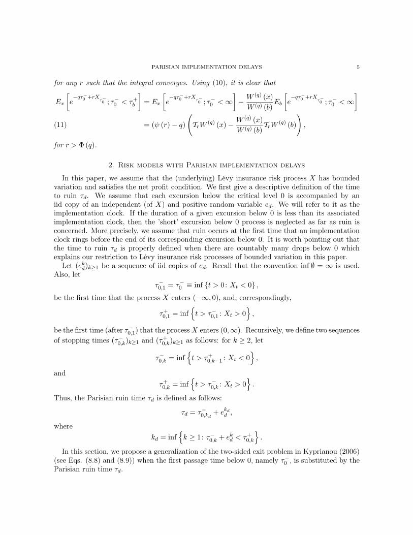
for any r such that the integral converges. Using (10), it is clear that

Ex

[e−qτ−0 +rX

τ−0 ; τ−0 < τ+b

]= Ex

[e−qτ−0 +rX

τ−0 ; τ−0 <∞]− W (q) (x)W (q) (b)

Eb

[e−qτ−0 +rX

τ−0 ; τ−0 <∞]

= (ψ (r)− q)

(TrW (q) (x)− W (q) (x)

W (q) (b)TrW (q) (b)

),(11)

for r > Φ (q).

2. Risk models with Parisian implementation delays

In this paper, we assume that the (underlying) Lévy insurance risk process X has boundedvariation and satisfies the net profit condition. We first give a descriptive definition of the timeto ruin τd. We assume that each excursion below the critical level 0 is accompanied by aniid copy of an independent (of X) and positive random variable ed. We will refer to it as theimplementation clock. If the duration of a given excursion below 0 is less than its associatedimplementation clock, then the ’short’ excursion below 0 process is neglected as far as ruin isconcerned. More precisely, we assume that ruin occurs at the first time that an implementationclock rings before the end of its corresponding excursion below 0. It is worth pointing out thatthe time to ruin τd is properly defined when there are countably many drops below 0 whichexplains our restriction to Lévy insurance risk processes of bounded variation in this paper.

Let (ekd)k≥1 be a sequence of iid copies of ed. Recall that the convention inf ∅ = ∞ is used.Also, let

τ−0,1 = τ−0 ≡ inf t > 0: Xt < 0 ,

be the first time that the process X enters (−∞, 0), and, correspondingly,

τ+0,1 = inf

t > τ−0,1 : Xt > 0

,

be the first time (after τ−0,1) that the processX enters (0,∞). Recursively, we define two sequencesof stopping times (τ−0,k)k≥1 and (τ+

0,k)k≥1 as follows: for k ≥ 2, let

τ−0,k = inft > τ+

0,k−1 : Xt < 0,

andτ+

0,k = inft > τ−0,k : Xt > 0

.

Thus, the Parisian ruin time τd is defined as follows:

τd = τ−0,kd + ekdd ,

wherekd = inf

k ≥ 1: τ−0,k + ekd < τ+

0,k

.

In this section, we propose a generalization of the two-sided exit problem in Kyprianou (2006)(see Eqs. (8.8) and (8.9)) when the first passage time below 0, namely τ−0 , is substituted by theParisian ruin time τd.


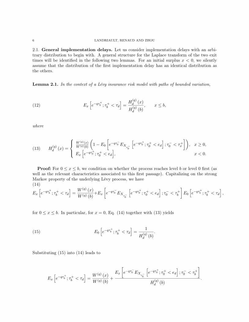
2.1. General implementation delays. Let us consider implementation delays with an arbi-trary distribution to begin with. A general structure for the Laplace transform of the two exittimes will be identified in the following two lemmas. For an initial surplus x < 0, we silentlyassume that the distribution of the first implementation delay has an identical distribution asthe others.

Lemma 2.1. In the context of a Lévy insurance risk model with paths of bounded variation,

(12) Ex

[e−qτ

+b ; τ+

b < τd

]=H

(q)d (x)

H(q)d (b)

, x ≤ b,

where

(13) H(q)d (x) =

W (q)(x)

W (q)(0)

(1− E0

[e−qτ

−0 EX

τ−0

[e−qτ

+0 ; τ+

0 < ed

]; τ−0 < τ+

x

]), x ≥ 0,

Ex

[e−qτ

+0 ; τ+

0 < ed

], x < 0.

Proof: For 0 ≤ x ≤ b, we condition on whether the process reaches level b or level 0 first (aswell as the relevant characteristics associated to this first passage). Capitalizing on the strongMarkov property of the underlying Lévy process, we have(14)

Ex

[e−qτ

+b ; τ+

b < τd

]=W (q) (x)W (q) (b)

+Ex

[e−qτ

−0 EX

τ−0

[e−qτ

+0 ; τ+

0 < ed

]; τ−0 < τ+

b

]E0

[e−qτ

+b ; τ+

b < τd

],

for 0 ≤ x ≤ b. In particular, for x = 0, Eq. (14) together with (13) yields

(15) E0

[e−qτ

+b ; τ+

b < τd

]=

1

H(q)d (b)

.

Substituting (15) into (14) leads to

Ex

[e−qτ

+b ; τ+

b < τd

]=W (q) (x)W (q) (b)

+Ex

[e−qτ

−0 EX

τ−0

[e−qτ

+0 ; τ+

0 < ed

]; τ−0 < τ+

b

]H

(q)d (b)

.


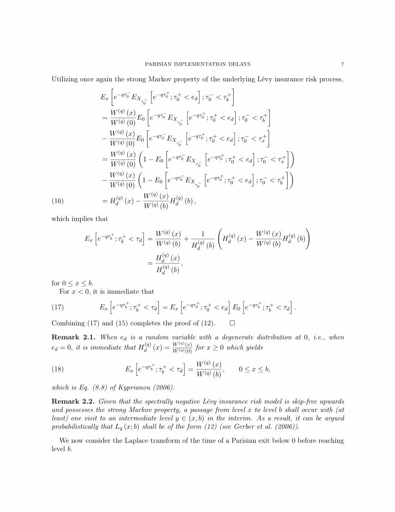
Utilizing once again the strong Markov property of the underlying Lévy insurance risk process,

Ex

[e−qτ

−0 EX

τ−0

[e−qτ

+0 ; τ+

0 < ed

]; τ−0 < τ+

b

]=W (q) (x)W (q) (0)

E0

[e−qτ

−0 EX

τ−0

[e−qτ

+0 ; τ+

0 < ed

]; τ−0 < τ+

b

]− W (q) (x)W (q) (0)

E0

[e−qτ

−0 EX

τ−0

[e−qτ

+0 ; τ+

0 < ed

]; τ−0 < τ+

x

]=W (q) (x)W (q) (0)

(1− E0

[e−qτ

−0 EX

τ−0

[e−qτ

+0 ; τ+

0 < ed

]; τ−0 < τ+

x

])− W (q) (x)W (q) (0)

(1− E0

[e−qτ

−0 EX

τ−0

[e−qτ

+0 ; τ+

0 < ed

]; τ−0 < τ+

b

])= H

(q)d (x)− W (q) (x)

W (q) (b)H

(q)d (b) ,(16)

which implies that

Ex

[e−qτ

+b ; τ+

b < τd

]=W (q) (x)W (q) (b)

+1

H(q)d (b)

(H

(q)d (x)− W (q) (x)

W (q) (b)H

(q)d (b)

)

=H

(q)d (x)

H(q)d (b)

,

for 0 ≤ x ≤ b.For x < 0, it is immediate that

(17) Ex

[e−qτ

+b ; τ+

b < τd

]= Ex

[e−qτ

+0 ; τ+

0 < ed

]E0

[e−qτ

+b ; τ+

b < τd

].

Combining (17) and (15) completes the proof of (12).

Remark 2.1. When ed is a random variable with a degenerate distribution at 0, i.e., whened = 0, it is immediate that H(q)

d (x) = W (q)(x)

W (q)(0)for x ≥ 0 which yields

(18) Ex

[e−qτ

+b ; τ+

b < τd

]=W (q) (x)W (q) (b)

, 0 ≤ x ≤ b,

which is Eq. (8.8) of Kyprianou (2006).

Remark 2.2. Given that the spectrally negative Lévy insurance risk model is skip-free upwardsand possesses the strong Markov property, a passage from level x to level b shall occur with (atleast) one visit to an intermediate level y ∈ (x, b) in the interim. As a result, it can be arguedprobabilistically that Lq (x; b) shall be of the form (12) (see Gerber et al. (2006)).

We now consider the Laplace transform of the time of a Parisian exit below 0 before reachinglevel b.


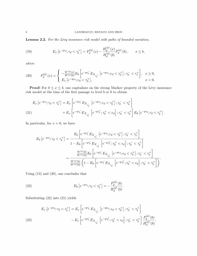
Lemma 2.2. For the Lévy insurance risk model with paths of bounded variation,

(19) Ex[e−qτd ; τd < τ+

b

]= P

(q)d (x)−

H(q)d (x)

H(q)d (b)

P(q)d (b) , x ≤ b,

where

(20) P(q)d (x) =

−W (q)(x)

W (q)(0)E0

[e−qτ

−0 EX

τ−0

[e−qed ; ed < τ+

0

]; τ−0 < τ+

x

], x ≥ 0,

Ex[e−qed ; ed < τ+

0

], x < 0.

Proof: For 0 ≤ x ≤ b, one capitalizes on the strong Markov property of the Lévy insurancerisk model at the time of the first passage to level b or 0 to obtain

Ex[e−qτd ; τd < τ+

b

]= Ex

[e−qτ

−0 EX

τ−0

[e−qed ; ed < τ+

0

]; τ−0 < τ+

b

]+ Ex

[e−qτ

−0 EX

τ−0

[e−qτ

+0 ; τ+

0 < ed

]; τ−0 < τ+

b

]E0

[e−qτd ; τd < τ+

b

].(21)

In particular, for x = 0, we have

E0


b

]=

E0

[e−qτ

−0 EX

τ−0

[e−qed ; ed < τ+

0

]; τ−0 < τ+

b

]1− E0

[e−qτ

−0 EX

τ−0

[e−qτ

+0 ; τ+

0 < ed

]; τ−0 < τ+

b

]

=

W (q)(b)

W (q)(0)E0

[e−qτ

−0 EX

τ−0

[e−qed ; ed < τ+

0

]; τ−0 < τ+

b

]W (q)(b)

W (q)(0)

(1− E0

[e−qτ

−0 EX

τ−0

[e−qτ

+0 ; τ+

0 < ed

]; τ−0 < τ+

b

]) .

Using (13) and (20), one concludes that

(22) E0


b

]= −

P(q)d (b)

H(q)d (b)

.

Substituting (22) into (21) yields


b

]= Ex

[e−qτ

−0 EX

τ−0

[e−qed ; ed < τ+

0

]; τ−0 < τ+

b

]− Ex

[e−qτ

−0 EX

τ−0

[e−qτ

+0 ; τ+

0 < ed

]; τ−0 < τ+

b

]P

(q)d (b)

H(q)d (b)

.(23)


Using sample path arguments, it can be shown that

Ex

[e−qτ

−0 EX

τ−0

[e−qed ; ed < τ+

0

]; τ−0 < τ+

b

]=W (q) (x)W (q) (0)

E0

[e−qτ

−0 EX

τ−0

[e−qed ; ed < τ+

0

]; τ−0 < τ+

b

]− W (q) (x)W (q) (0)

E0

[e−qτ

−0 EX

τ−0

[e−qed ; ed < τ+

0

]; τ−0 < τ+

x

]= P

(q)d (x)− W (q) (x)

W (q) (b)P

(q)d (b) .(24)

Using (16) and (24), (23) becomes


b

]= P

(q)d (x)− W (q) (x)

W (q) (b)P

(q)d (b)−

(H

(q)d (x)

H(q)d (b)

− W (q) (x)W (q) (b)

)P

(q)d (b)

= P(q)d (x)−

H(q)d (x)

H(q)d (b)

P(q)d (b) .(25)

For x < 0, we condition on whether the implementation clock or the first passage to level 0will occur first. It follows that

(26) Ex[e−qτd ; τd < τ+

b

]= Ex

[e−qed ; ed < τ+

0

]+ Ex

[e−qτ

+0 ; τ+

0 < ed

]E0


b

].

Using (22) and (13), (26) becomes


b

]= Ex

[e−qed ; ed < τ+

0

]−H(q)

d (x)P

(q)d (b)

H(q)d (b)

.

From the definition of P (q)d (x) for x < 0, the proof is now complete.

Remark 2.3. Assuming that ed is a random variable with a degenerate distribution at 0, wehave

(27) P(q)d (x) = −W

(q) (x)W (q) (0)

E0

[e−qτ

−0 ; τ−0 < τ+

x

], x > 0.

With the help of (9), (27) can be rewritten as

(28) P(q)d (x) = Z(q) (x)− W (q) (x)

W (q) (0).

Substituting (28) and (18) into (19)


b

]= Z(q) (x)− W (q) (x)

W (q) (0)− W (q) (x)W (q) (b)

(Z(q) (b)− W (q) (b)

W (q) (0)

)

= Z(q) (x)− W (q) (x)W (q) (b)

Z(q) (b) ,

for x ≥ 0, which is Eq. (8.9) of Kyprianou (2006).


In what follows, we characterize H(q)d and P

(q)d in the representation of the two-sided exit

problem when implementation delays are exponentially distributed and mixed Erlang distributedrespectively.

2.2. Exponentially distributed implementation delays. Let ed be an exponentially dis-tributed random variable with mean 1/β. From Theorem 3.12 of Kyprianou (2006), it is clearthat, for x < 0,

(29) Ex

[e−qτ

+0 ; τ+

0 < ed

]= eΦ(q+β)x.


(30) H(q)d (x) =

W (q)(x)

W (q)(0)

(1− E0

[e−qτ−0 +Φ(q+β)X

τ−0 ; τ−0 < τ+x

]), x ≥ 0,

eΦ(q+β)x, x < 0.

Using (11) and (2), it is well known that

E0

[e−qτ−0 +Φ(q+β)X

τ−0 ; τ−0 < τ+x

]= β

TΦ(q+β)W

(q) (0)− W (q) (0)W (q) (x)

TΦ(q+β)W(q) (x)

= 1− βW(q) (0)

W (q) (x)TΦ(q+β)W

(q) (x) ,(31)

for x ≥ 0. Combining (30) and (31) results in

(32) H(q)d (x) =

βTΦ(q+β)W

(q) (x), x ≥ 0,eΦ(q+β)x, x < 0.

As for P (q)d , it is easy to show that, for x > 0,


0

]= E

[e−qed

]− Ex

[e−qτ

+0 ; τ+

0 < ed

]E[e−qed

]=

β

β + q

(1− eΦ(q+β)x

).(33)


(34) P(q)d (x) =

− ββ+q

W (q)(x)

W (q)(0)E0

[e−qτ

−0

(1− e

Φ(q+β)Xτ−0

); τ−0 < τ+

x

], x ≥ 0,

ββ+q

(1− eΦ(q+β)x

), x < 0.

With the help of (9) and (31),

E0

[e−qτ

−0

(1− e

Φ(q+β)Xτ−0

); τ−0 < τ+

x

]=

(1− W (q) (0)

W (q) (x)Z(q) (x)

)−

(1− βW

(q) (0)W (q) (x)

TΦ(q+β)W(q) (x)

)

=W (q) (0)W (q) (x)

(βTΦ(q+β)W

(q) (x)− Z(q) (x)),


which implies that (34) becomes

(35) P(q)d (x) =

ββ+q

(Z(q) (x)− βTΦ(q+β)W

(q) (x)), x ≥ 0,

ββ+q

(1− eΦ(q+β)x

), x < 0.

By extending the domain of definition of Z(q) such that Z(q) (x) = 1 for x < 0, one concludes,by comparing (32) and (35), that

P(q)d (x) =

β

β + q

(Z(q) (x)−H(q)

d (x)),

which, in turn, yields


b

]=

β

β + q

(Z(q) (x)−

H(q)d (x)

H(q)d (b)

Z(q) (b)

).

2.3. Mixed Erlang implementation delays. We now generalize the results of Section 2.2 byassuming that ed is mixed Erlang distributed with Laplace transform

(36) f (s) = C

(β

β + s

),

where

C (z) =r∑

n=1

cnzn,

with cn ≥ 0 for n = 1, ..., r and∑r

n=1 cn = 1. Its survival function is given by

(37) F (x) =r−1∑n=0

Cn(βx)n

n!e−βx, x > 0,

where Cn =∑r

j=n+1 cj . We point out that the integer-valued parameter r can either be finiteor infinite. The reader is referred to Tijms (1994) for a proof that any positive and continuousrandom variable can be approximated arbitrary accurately by a mixed Erlang density and toWillmot and Woo (2007) for an extensive treatment of this class of distributions.

The following lemma will be helpful to characterize both H(q)d and P (q)

d in our generalizationof the two-sided exit problem. The proof is provided in the Appendix. In order to state theseresults, we first present a combinatorial identity known as di Bruno’s formula (see e.g. Riordan(1980)).

Proposition 2.1. (di Bruno’s formula) For two functions f and g sufficiently differentiable,

(38)dn

dθnf (g (θ)) =

n∑i=0

f (i) (g (θ))Bi,n(g(1) (θ) , g(2) (θ) , ..., g(n−i+1) (θ)

),

where Bi,n (x1, ..., xn−i+1) is the Bell polynomial

Bi,n (x1, ..., xn−i+1) =∑ n!

k1! k2! ... kn−i+1!

(x1

1!

)k1 (x2

2!

)k2...

(xn−i+1

(n− i+ 1)!

)kn−i+1

,


with the sum extends over all sequences k1, k2, ..., kn−i+1 of non-negative integers such that k1 +k2 + ...+ kn−i+1 = i and k1 + 2k2 + ...+ (n− i+ 1) kn−i+1 = n. By definition, let B0,0 (x1) = 1for all x1.

Lemma 2.3. For ed a mixed Erlang random variable with Laplace transform (36),

(39) Ex

[e−qτ

+0 ; τ+

0 < ed

]=

r−1∑i=0

ζi

xieΦ(q+β)x

, x < 0,

and

(40) Ex[e−qed ; ed < τ+

0

]= C

(β

β + q

)−

r−1∑i=0

χi

xieΦ(q+β)x

, x < 0,

where

ζi =r−1∑n=i

Cnϑi,n,

χi =r−1∑j=i

ϑi,j

r∑n=j+1

cn

(β

β + q

)n−j,

andϑi,n =

βn

n!(−1)nBi,n

(Φ(1) (q + β) , ...,Φ(n−i+1) (q + β)

).

Letbr,l,i = q1l=i −

(i

l

)ψ(i−l) (r) .

An explicit expression for H(q)d and P (q)

d is presented in the following proposition. The reader isreferred to the Appendix for the proof of this result.

Proposition 2.2. When ed has Laplace transform (36),(a)

(41) H(q)d (x) =

r−1∑l=0

νl

T l+1

Φ(q+β)W(q) (x)

, x ≥ 0,

r−1∑i=0

ζixieΦ(q+β)x

, x < 0,

where

(42) νl = (−1)l+1 (l!)r−1∑i=l

ζibΦ(q+β),l,i.

(b)

P(q)d (x) =

χ0−C

“ββ+q

”W (q)(0)

W (q) (x) + C(

ββ+q

)Z(q) (x) +

r−1∑l=0

ςl

T l+1

Φ(q+β)W(q) (x)

, x ≥ 0,

C(

ββ+q

)−r−1∑i=0

χixieΦ(q+β)x

, x < 0,

(43)


where

ςl = (−1)l (l!)r−1∑i=l

χibΦ(q+β),l,i.

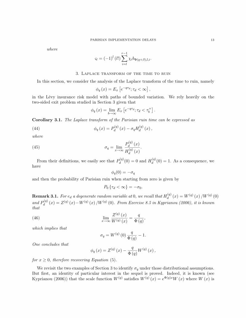
3. Laplace transform of the time to ruin

In this section, we consider the analysis of the Laplace transform of the time to ruin, namely

φq (x) = Ex[e−qτd ; τd <∞

],

in the Lévy insurance risk model with paths of bounded variation. We rely heavily on thetwo-sided exit problem studied in Section 3 given that

φq (x) = limb→∞


b

].

Corollary 3.1. The Laplace transform of the Parisian ruin time can be expressed as

(44) φq (x) = P(q)d (x)− σqH(q)

d (x) ,

where

(45) σq = limx→∞

P(q)d (x)

H(q)d (x)

.

From their definitions, we easily see that P (q)d (0) = 0 and H(q)

d (0) = 1. As a consequence, wehave

φq(0) = −σqand then the probability of Parisian ruin when starting from zero is given by

P0 τd <∞ = −σ0.

Remark 3.1. For ed a degenerate random variable at 0, we recall that H(q)d (x) = W (q) (x) /W (q) (0)

and P (q)d (x) = Z(q) (x)−W (q) (x) /W (q) (0). From Exercise 8.5 in Kyprianou (2006), it is known

that

(46) limx→∞

Z(q) (x)W (q) (x)

=q

Φ (q),

which implies that

σq = W (q) (0)q

Φ (q)− 1.

One concludes thatφq (x) = Z(q) (x)− q

Φ (q)W (q) (x) ,

for x ≥ 0, therefore recovering Equation (5).

We revisit the two examples of Section 3 to identify σq under those distributional assumptions.But first, an identity of particular interest in the sequel is proved. Indeed, it is known (seeKyprianou (2006)) that the scale function W (q) satisfies W (q) (x) = eΦ(q)xW (x) where W (x) is


a non-decreasing and bounded function, the latter being provided by the net profit condition.As a result,

T lrW (q) (x)W (q) (x)

=∫ ∞

0

yl−1e−ry

(l − 1)!W (q) (x+ y)W (q) (x)

dy

=∫ ∞

0

yl−1e−(r−Φ(q))y

(l − 1)!W (x+ y)W (x)

dy.

for l = 1, 2, ... and r > Φ (q). Letting x → ∞ and using the dominated convergence theorem,one concludes that

limx→∞

T lrW (q) (x)W (q) (x)

=∫ ∞

0

yl−1e−(r−Φ(q))y

(l − 1)!dy

=(

1r − Φ (q)

)l,(47)

for l = 1, 2, ... and r > Φ (q).

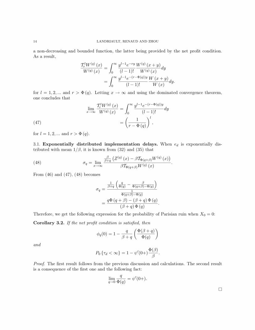
3.1. Exponentially distributed implementation delays. When ed is exponentially dis-tributed with mean 1/β, it is known from (32) and (35) that

(48) σq = limx→∞

ββ+q

(Z(q) (x)− βTΦ(q+β)W

(q) (x))

βTΦ(q+β)W (q) (x).

From (46) and (47), (48) becomes

σq =1

β+q

(q

Φ(q) −β

Φ(q+β)−Φ(q)

)1

Φ(q+β)−Φ(q)

=qΦ (q + β)− (β + q) Φ (q)

(β + q) Φ (q).

Therefore, we get the following expression for the probability of Parisian ruin when X0 = 0:

Corollary 3.2. If the net profit condition is satisfied, then

φq(0) = 1− q

β + q

(Φ(β + q)

Φ(q)

)and

P0 τd <∞ = 1− ψ′(0+)Φ(β)β

.

Proof. The first result follows from the previous discussion and calculations. The second resultis a consequence of the first one and the following fact:

limq→0

q

Φ(q)= ψ′(0+).


3.2. Mixed Erlang implementation delays. Similarly, when ed is a mixed Erlang randomvariable with Laplace transform (36), it is known from Proposition 2.2 that

(49) σq = limx→∞

χ0−C“

ββ+q

”W (q)(0)

W (q) (x) + C(

ββ+q

)Z(q) (x) +

r−1∑l=0

ςl

T l+1

Φ(q+β)W(q) (x)

r−1∑l=0

νl

T l+1

Φ(q+β)W(q) (x)

.

From (46) and (47), (49) becomes

σq =

χ0−C“

ββ+q

”W (q)(0)

+ C(

ββ+q

)q

Φ(q) +r−1∑l=0

ςl

(1

Φ(q+β)−Φ(q)

)l+1

r−1∑l=0

νl

(1

Φ(q+β)−Φ(q)

)l+1.

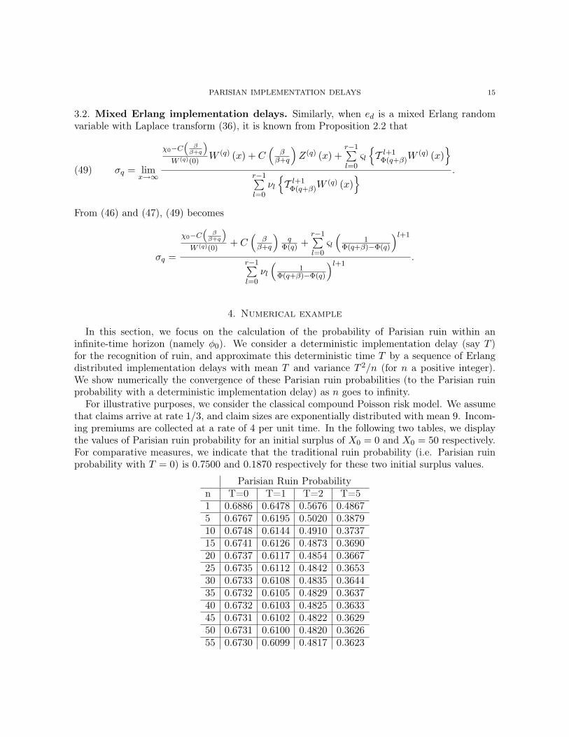
4. Numerical example

In this section, we focus on the calculation of the probability of Parisian ruin within aninfinite-time horizon (namely φ0). We consider a deterministic implementation delay (say T )for the recognition of ruin, and approximate this deterministic time T by a sequence of Erlangdistributed implementation delays with mean T and variance T 2/n (for n a positive integer).We show numerically the convergence of these Parisian ruin probabilities (to the Parisian ruinprobability with a deterministic implementation delay) as n goes to infinity.

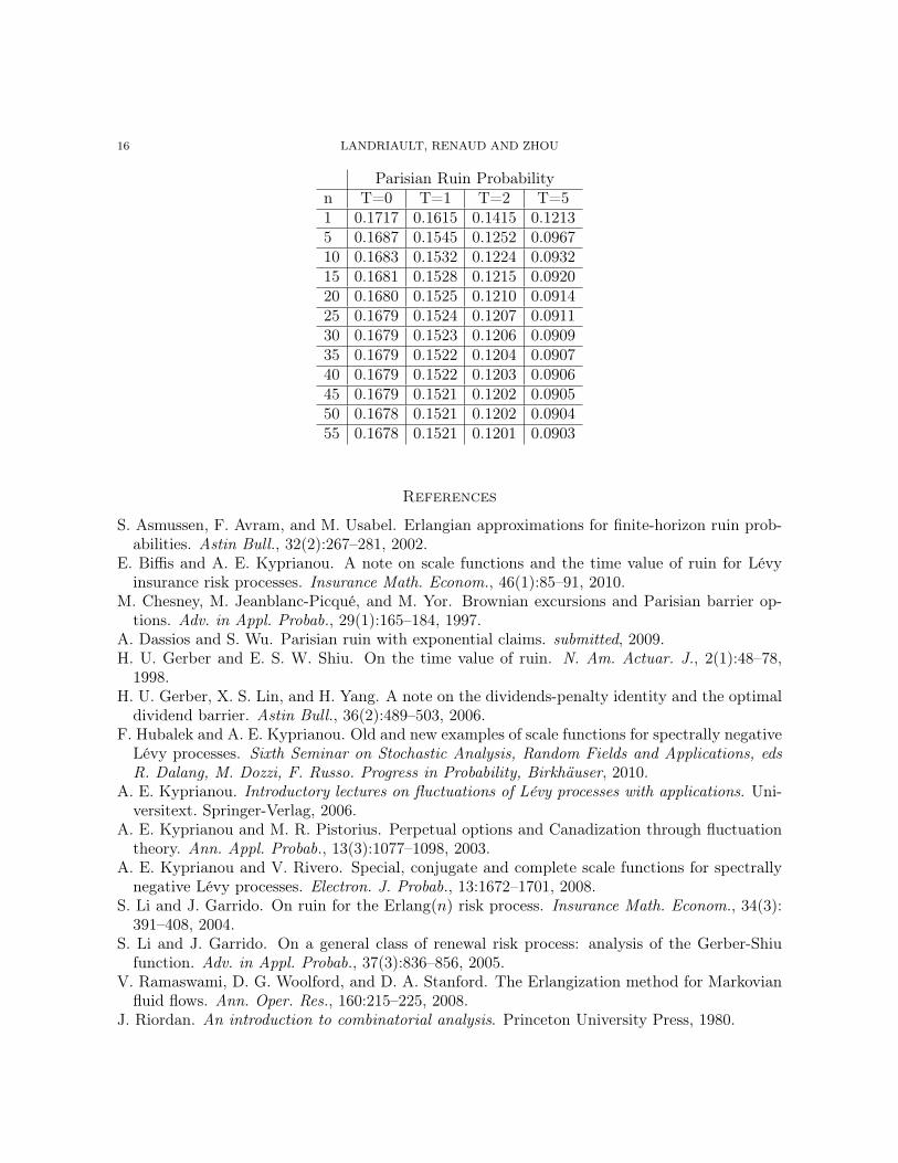
For illustrative purposes, we consider the classical compound Poisson risk model. We assumethat claims arrive at rate 1/3, and claim sizes are exponentially distributed with mean 9. Incom-ing premiums are collected at a rate of 4 per unit time. In the following two tables, we displaythe values of Parisian ruin probability for an initial surplus of X0 = 0 and X0 = 50 respectively.For comparative measures, we indicate that the traditional ruin probability (i.e. Parisian ruinprobability with T = 0) is 0.7500 and 0.1870 respectively for these two initial surplus values.

Parisian Ruin Probabilityn T=0 T=1 T=2 T=51 0.6886 0.6478 0.5676 0.48675 0.6767 0.6195 0.5020 0.387910 0.6748 0.6144 0.4910 0.373715 0.6741 0.6126 0.4873 0.369020 0.6737 0.6117 0.4854 0.366725 0.6735 0.6112 0.4842 0.365330 0.6733 0.6108 0.4835 0.364435 0.6732 0.6105 0.4829 0.363740 0.6732 0.6103 0.4825 0.363345 0.6731 0.6102 0.4822 0.362950 0.6731 0.6100 0.4820 0.362655 0.6730 0.6099 0.4817 0.3623


Parisian Ruin Probabilityn T=0 T=1 T=2 T=51 0.1717 0.1615 0.1415 0.12135 0.1687 0.1545 0.1252 0.096710 0.1683 0.1532 0.1224 0.093215 0.1681 0.1528 0.1215 0.092020 0.1680 0.1525 0.1210 0.091425 0.1679 0.1524 0.1207 0.091130 0.1679 0.1523 0.1206 0.090935 0.1679 0.1522 0.1204 0.090740 0.1679 0.1522 0.1203 0.090645 0.1679 0.1521 0.1202 0.090550 0.1678 0.1521 0.1202 0.090455 0.1678 0.1521 0.1201 0.0903

References

S. Asmussen, F. Avram, and M. Usabel. Erlangian approximations for finite-horizon ruin prob-abilities. Astin Bull., 32(2):267–281, 2002.

E. Biffis and A. E. Kyprianou. A note on scale functions and the time value of ruin for Lévyinsurance risk processes. Insurance Math. Econom., 46(1):85–91, 2010.

M. Chesney, M. Jeanblanc-Picqué, and M. Yor. Brownian excursions and Parisian barrier op-tions. Adv. in Appl. Probab., 29(1):165–184, 1997.

A. Dassios and S. Wu. Parisian ruin with exponential claims. submitted, 2009.H. U. Gerber and E. S. W. Shiu. On the time value of ruin. N. Am. Actuar. J., 2(1):48–78,

1998.H. U. Gerber, X. S. Lin, and H. Yang. A note on the dividends-penalty identity and the optimaldividend barrier. Astin Bull., 36(2):489–503, 2006.

F. Hubalek and A. E. Kyprianou. Old and new examples of scale functions for spectrally negativeLévy processes. Sixth Seminar on Stochastic Analysis, Random Fields and Applications, edsR. Dalang, M. Dozzi, F. Russo. Progress in Probability, Birkhäuser, 2010.

A. E. Kyprianou. Introductory lectures on fluctuations of Lévy processes with applications. Uni-versitext. Springer-Verlag, 2006.

A. E. Kyprianou and M. R. Pistorius. Perpetual options and Canadization through fluctuationtheory. Ann. Appl. Probab., 13(3):1077–1098, 2003.

A. E. Kyprianou and V. Rivero. Special, conjugate and complete scale functions for spectrallynegative Lévy processes. Electron. J. Probab., 13:1672–1701, 2008.

S. Li and J. Garrido. On ruin for the Erlang(n) risk process. Insurance Math. Econom., 34(3):391–408, 2004.

S. Li and J. Garrido. On a general class of renewal risk process: analysis of the Gerber-Shiufunction. Adv. in Appl. Probab., 37(3):836–856, 2005.

V. Ramaswami, D. G. Woolford, and D. A. Stanford. The Erlangization method for Markovianfluid flows. Ann. Oper. Res., 160:215–225, 2008.

J. Riordan. An introduction to combinatorial analysis. Princeton University Press, 1980.


B. A. Surya. Evaluating scale functions of spectrally negative Lévy processes. J. Appl. Probab.,45(1):135–149, 2008.

H. C. Tijms. Stochastic models. John Wiley & Sons Ltd., 1994.G. E. Willmot. On the discounted penalty function in the renewal risk model with generalinterclaim times. Insurance Math. Econom., 41(1):17–31, 2007.

G. E. Willmot and J.-K. Woo. On the class of Erlang mixtures with risk theoretic applications.N. Am. Actuar. J., 11(2):99–115, 2007.

5. Appendix

5.1. Proof of (39) in Lemma 2.3. Using the mixed Erlang survival function (37), one readilyfinds

Ex

[e−qτ

+0 ; τ+

0 < ed

]= Ex

[e−qτ

+0

(r−1∑n=0

Cn

(βτ+

0

)nn!

e−βτ+0

); τ+

0 <∞

]

=r−1∑n=0

Cnβn

n!Ex

[(τ+

0

)ne−(q+β)τ+

0 ; τ+0 <∞

]=

r−1∑n=0

Cnβn

n!(−1)n Ex

[dn

dξne−ξτ

+0 ; τ+

0 <∞]∣∣∣∣ξ=q+β

,

for x ≥ 0. Interchanging the order of the expectation sign and the n-th derivative, one finds that

(50) Ex

[e−qτ

+0 ; τ+

0 < ed

]=

r−1∑n=0

Cnβn

n!(−1)n

dn

dξneΦ(ξ)x

∣∣∣∣ξ=q+β

Using di Bruno’s formula, (50) becomes(51)

Ex

[e−qτ

+0 ; τ+

0 < ed

]= eΦ(q+β)x

r−1∑n=0

Cnβn

n!(−1)n

n∑i=0

xiBi,n

(Φ(1) (q + β) , ...,Φ(n−i+1) (q + β)

),

Interchanging the order of summation in (51) leads to (39).

5.2. Proof of (40) in Lemma 2.3. Using the mixed Erlang density followed by a series ofsimple manipulations, one arrives at


0

]=

r∑n=1

cnEx[e−qen,β ; en,β < τ+

0

]=

r∑n=1

cn(E[e−qen,β

]− Ex

[e−qen,β ; τ+

0 < en,β])

=r∑

n=1

cn

E [e−qen,β]− n−1∑j=0

Ex[e−qen,β ; ej,β < τ+

0 < ej+1,β

] ,(52)


where ej,β is an Erlang-j random variable with density

f (y) =βjyj−1e−βy

(j − 1)!, y > 0,

(with e0,β a degenerate random variable at 0). Given that the Lévy insurance risk model isskip-free upwards and due to the memoryless property of the exponential distribution, we have

(53) Ex[e−qen,β ; ej,β < τ+

0 < ej+1,β

]= Ex

[e−qτ

+0 E

[e−qen−j,β

]; ej,β < τ+

0 < ej+1,β

],

where

(54) E[e−qej,µ

]=(

β

β + q

)j, j = 0, 1, 2, ...

Substituting (53) and (54) into (52) yields


0

]= C

(β

β + q

)−

r∑n=1

cn

n−1∑j=0

(β

β + q

)n−jEx

[e−qτ

+0 ; ej,β < τ+

0 < ej+1,β

].

(55)

Using (39) with

Cn =

1, n = 0, 1, ..., j,0, n = j + 1, j + 2, ...,

and

Cn =

1, n = 0, 1, ..., j − 1,0, n = j, j + 1, ...,

respectively, one deduces that

Ex

[e−qτ

+0 ; ej,β < τ+

0 < ej+1,β

]= Ex

[e−qτ

+0 ; τ+

0 < ej+1,β

]− Ex

[e−qτ

+0 ; τ+

0 < ej,β

]=

j∑i=0

ϑi,j

xieΦ(q+β)x

.(56)

Substituting (56) into (55) (followed by some simple manipulations) yields (40).

5.3. Proof of Proposition 2.2. For x < 0, (41) and (43) follows immediately from Lemma 2.3together with (13) and (20) respectively. For x ≥ 0, the results of Lemma 2.3 allows to rewrite(13) and (20) respectively as

(57) H(q)d (x) =

W (q) (x)W (q) (0)

(1−

r−1∑i=0

ζi E0

[(Xτ−0

)ie−qτ−0 +Φ(q+β)X

τ−0 ; τ−0 < τ+x

]),


and

P(q)d (x) =

W (q) (x)W (q) (0)

r−1∑i=0

χiE0

[(Xτ−0

)ie−qτ−0 +Φ(β+q)X

τ−0

; τ−0 < τ+

x

]

− W (q) (x)W (q) (0)

C

(β

β + q

)E0

[e−qτ

−0 ; τ−0 < τ+

x

].(58)

An expression for E0

[(Xτ−0

)ie−qτ−0 +rX

τ−0 ; τ−0 < τ+x

]for r > Φ (q) is needed to further explicit

(57) and (58).For i = 0, (11) immediately yields

(59) E0

[e−qτ−0 +rX

τ−0 ; τ−0 < τ+x

]= 1−W (q) (0) (ψ (r)− q) TrW

(q) (x)W (q) (x)

.

Otherwise, for i = 1, 2, ...,

E0

[(Xτ−0

)ie−qτ−0 +rX

τ−0 ; τ−0 < τ+x

]=

di

dξiE0

[e−qτ−0 +ξX

τ−0 ; τ−0 < τ+x

]∣∣∣∣ξ=r

= W (q) (0)di

dξi

((q − ψ (ξ))

TξW (q) (x)W (q) (x)

)∣∣∣∣∣ξ=r

.(60)

From Property 5 of the Dickson-Hipp operator on page 393 of Li and Garrido (2004), namely

dl

dξlTξW (q) (x) = (−1)l (l!) T l+1

ξ W (q) (x) , l = 0, 1, ...,

(60) becomes

(61) E0

[(Xτ−0

)ie−qτ−0 +rX

τ−0 ; τ−0 < τ+x

]= W (q) (0)

i∑l=0

br,l,i(−1)l (l!) T l+1

r W (q) (x)W (q) (x)

,

for r > Φ (q) where

br,l,i = q1l=i −(i

l

)ψ(i−l) (r) .

Then, substituting (59) and (61) into (57) and using the fact that ζ0 = 1, one concludes that

H(q)d (x) =

W (q) (x)W (q) (0)

(1− ζ0

(1− βW (q) (0)

TΦ(q+β)W(q) (x)

W (q) (x)

))

−r−1∑i=1

ζi

i∑l=0

bΦ(q+β),l,i

(−1)l (l!) T l+1

Φ(q+β)W(q) (x)

= βTΦ(q+β)W

(q) (x) +r−1∑i=1

ζi

i∑l=0

bΦ(q+β),l,i

(−1)l+1 (l!) T l+1

Φ(q+β)W(q) (x)

=

r−1∑i=0

ζi

i∑l=0

bΦ(q+β),l,i

(−1)l+1 (l!) T l+1

Φ(q+β)W(q) (x)

.(62)


Interchanging the order of summation, (62) has the equivalent representation given in (41). Usinga similar line of logic, (43) can be obtained from (58) through (59), (61) and (9). The proof istherefore omitted.

5.4. Derivatives of Φ (θ). In this section, we propose a recursive formula for the calculation ofthe derivatives of the inverse of the Laplace exponent, namely Φ (θ). Under the positive securityloading condition, we have

(63) θ = ψ (Φ (θ)) .

Using the chain rule, the differentiation of (63) w.r.t. θ yields

1 = ψ′ (Φ (θ)) Φ′ (θ) ,

or equivalently

Φ′ (θ) =1

ψ′ (Φ (θ)).

In general, the same procedure can be repeated to obtain the higher-order derivatives of Φ (θ).Indeed, using di Bruno’s formula (see Eq. (38)), we have

(64)dn

dθnψ (Φ (θ)) =

n∑i=1

ψ(i) (Φ (θ))Bi,n(

Φ(1) (θ) ,Φ(2) (θ) , ...,Φ(n−i+1) (θ)),

where Bi,n is the Bell polynomial. It is easy to show that B1,n (x1, ..., xn) = xn which permitsto re-write (64) as(65)dn

dθnψ (Φ (θ)) = ψ(1) (Φ (θ)) Φ(n) (θ) +

n∑i=2


Φ(1) (θ) ,Φ(2) (θ) , ...,Φ(n−i+1) (θ)),

where it is worth pointing out that the second term on the right-hand side of (65) is a functionof the first (n− 1) derivatives of Φ (θ). For n ≥ 2, an application of the n-th derivative operatoron each side of (63) results in

0 = ψ(1) (Φ (θ)) Φ(n) (θ) +n∑i=2


Φ(1) (θ) ,Φ(2) (θ) , ...,Φ(n−i+1) (θ)),

or equivalently

Φ(n) (θ) =−1

ψ(1) (Φ (θ))

(n∑i=2


Φ(1) (θ) ,Φ(2) (θ) , ...,Φ(n−i+1) (θ)))

=(−Φ′ (θ)

) n∑i=2


Φ(1) (θ) ,Φ(2) (θ) , ...,Φ(n−i+1) (θ)).(66)


Department of Statistics and Actuarial Science, University of Waterloo, 200 University Av-enue West, Waterloo (Ontario) N2L 3G1, Canada

E-mail address: [email protected]

Département de mathématiques, UQAM, 201 av. Président-Kennedy, Montréal (Québec) H2X3Y7, Canada


Department of Mathematics and Statistics, Concordia University, 1455 de Maisonneuve BlvdW., Montréal (Québec) H3G 1M8, Canada


INSURANCE RISK MODELS WITH PARISIAN IMPLEMENTATION …

Documents

Transcript of INSURANCE RISK MODELS WITH PARISIAN IMPLEMENTATION …